
Abstract
Proton exchange membrane fuel cell (PEMFC) is considered as propitious solution for an environmentally friendly energy source. A precise model of PEMFC for accurate identification of its polarization curve and in-depth understanding of all its operating characteristics attracted the interest of many researchers. In this paper, novel meta-heuristic optimization methods have been successfully applied to evaluate the unknown parameters of PEMFC models, particularly Harris Hawks’ optimization (HHO) and atom search optimization (ASO) techniques. The proposed optimization algorithms have been tested on three different commercial PEMFC stacks, namely BCS 500-W PEM, 500W SR-12PEM and 250W stack, under various operating conditions. The sum of square errors (SSE) between the results obtained by the application of the estimated parameters and the experimentally measured results of the fuel cell stacks was considered as the objective function of the optimization problem. In order to validate the effectiveness of the proposed methods, the results are compared with that obtained in studies. Moreover, the I/V curves obtained by the application of HHO and ASO showed a clear matching with data sheet curves for all the studied cases. Finally, PEMFC model based on HHO technique surpasses all compared algorithms in terms of the solution accuracy and the convergence speed.
1 Introduction
The greenhouse gases and the depletion of fossil fuels have provoked the governments and industries to invest more in renewable energy sources (RESs) such as PV, wind, tidal and wave. Utilizing such new RES into power grids takes new trends. It can be harnessed as a smart micro-grid or can be integrated as an isolated standalone AC–DC power grid [1]. However, due to its stochastic nature and during load peak hours, backup supports are needed. Fuel cells are an elegant choice which can play an important role in such upcoming power grids.
Since 1990, fuel cell development has progressed rapidly. Car manufactures and heating firms have discovered the technology and aim to benefit from its positive image. Fuel cell operation is based on chemical reaction that occurs under controlled conditions. A fuel cell consists of an electrode and a cathode with an electrolyte between them. The anode is fed by pure hydrogen (H2) or a flamed gas containing hydrogen, while oxygen (O2) or air is fed to the cathode. Depending on electrolyte, gases used as a fuel and the operating temperature, there are various classifications for the fuel cells. The polymer electrolyte fuel cell (PEFC) and proton exchange membrane fuel cell (PEMFC) are the most commonly used types. Its operating temperature is around 80 °C, and it can run on with normal air and reformed hydrogen as a fuel [2].
The mathematical model of the fuel cell is considered as the milestone on which the designing and testing of the fuel cell can be performed in an appropriate way. Moreover, a good mathematical model is essential to move forward the integration of the fuel cell besides supporting the designers with more information about the physical phenomena occurring inside it. The electrochemical model of the fuel cell has essential empirical and semiempirical equations that depend on a combination set of unknown parameters. The inherited coupled parameters make the modeling of a fuel cell more difficult, which motivate the researcher to search for a suitable solution. Due to its sufficient way to obtain optimum solutions for complicated problems, meta-heuristics can be adapted to provide robust parameter estimation for fuel cell modeling. From this fact, the no-free-lunch theorem has made a cogent remark that is employed by several optimization techniques to solve various engineering optimization problems [3, 4].
The adaptive differential evolution algorithm (ADE) is one of the competitive methods which have been used for solving the parameter estimation for PEMFC [5]. The main contribution of the proposed ADE method is to decrease the premature convergence and increase search efficiency. A hybrid adaptive differential evolution is introduced in [6]. It is a combination set between biological genetic strategy and bee colony foraging method. The first method enhances the parametric scaling for dynamic crossover probability, while the former method improves the weak local search. Hence, the ADE enhances the performance of the optimization techniques. A grouping-based global harmony search algorithm (GGHS) has been adopted for obtaining a precise estimation for PEMFC parameters as reported in [7]. The algorithm performance was compared with different methods such as particle swarm optimization (PSO) and seeker optimization algorithm (SOA). From comparison, it had been concluded that the GGHS platform exhibits better performance than other algorithms [7]. The genetic algorithm has been applied for parameter estimation of PEMFC [8,9,10]. In [8], a new formulation based on genetic algorithm (GA) is used to deal with fuel cell parameter evaluation. The main advantage of this method is lower complexity, less time consumption, enhancing accuracy and ease of implementation. A hybrid combination set between teaching learning-based optimization method (TLBO) and differential evaluation algorithm (DE) is introduced in [11] to obtain a proper estimation for the parameter model of PEMFC. The TLBO-DE performance is compared with different optimization algorithms. The TLBO-DE proves its accuracy and robustness, besides its ability to obtain optimum solution with lesser computation time. The gray wolf optimization (GWO) algorithm is used for identifying the PEMFC model parameters [12]. An experimental test is performed to prove a superior performance for GWO to other optimization methods such as antlion optimizer (ALO) and dragonfly algorithm (DA). New meta-heuristic approaches have been employed to adapt the PEMFC model parameter such as grasshopper optimization algorithm (GOA), salp swarm optimizer (SSO) and shark smell optimizer (SSO) [13,14,15]. The advantages of these methods are better convergence to optimum solution, tuning its controlling parameters with low effort of computation and faster process execution. In [16], JAYA algorithm was deployed to estimate the PEMFC parameters effectively. Compared to other optimization techniques, JAYA has better convergence time, accuracy and stability. In [17], the cuckoo search (CS) algorithm is used to obtain the parameters of the PEMFC. Author has proposed an explosion operator to fine tune the step size of the CS. The cuckoo search algorithm with explosion operator (CS-EO) proves its ability to avoid precipitate convergence and enhances the overall performance of the CS. Moreover, the application of multi-objective optimization algorithms of multi-objective genetic algorithm to handle the parameter estimation for PEMFCs has been discussed in [18]. All these algorithms are presented and applied for estimating the parameters of the PEMFC model for improving the estimation accuracy. However, most of these works could not strengthen the estimation accuracy. Therefore, it is necessary to present and validate recent methods which have the ability to accurately estimate the parameters of the PEMFC model with good convergence characteristics.
Recently, a contemporary optimization method has been proposed to solve complicated problems; this method is the atom search optimization (ASO) method. It is a simple structure method. Its advantages underlying, fewer controlling parameters, self-adaption to its parameters, can be adapted easily with other methods to obtain better convergence for optimal solutions [19]. However, this method is not deeply applied for solving electrical engineering problems. Moreover, one of the outstanding optimization techniques that have been discovered not a long time ago is the Harris Hawk optimization (HHO). Its performance is driven from the behavior of predator birds (“This species is called Harris’s hawk (Parabuteo unicinctus), but the algorithm is Harris Hawks Optimization algorithm”) [20]. It has a superior performance to act with the global optimization problems rather than the other optimization techniques. It possesses better exploration for the optimum solution without getting stacked to the local search.
In this paper, HHO and ASO have been used for estimating the parameters of a number of commercial proton exchange membrane fuel cells. To validate the effectiveness of the ASO- and HHO-based optimization methods, comparisons and different operating scenarios have been studied. The novelty in this work includes the implementation of two unprecedented optimization algorithms, namely HHO and ASO, for defining the equivocal parameters of fuel cell model and a comprehensive comparison with other competitive techniques provided in the literature.
2 Problem formulation
2.1 Basic physical operation
Fuel cells are considered as a direct method on converting the chemical energy into electrical energy. The construction of a typical proton exchange membrane (PEM) fuel cell is described in Fig. 1. As seen from the figure, the PEM fuel cell model comprises two electrodes (anode and cathode), between which a catalyst and a membrane layers are stacked. In addition, at the anode and cathode sides, two channels are used for supplying hydrogen and air, which will be diffused through the electrodes.

Electrode reactions and flow of charge in fuel cell
A simple way for understanding the base operation of the fuel cell is to say that the hydrogen gas is being “burnt” or combusted in the simple chemical reaction described as follows [21]:
However, in this case, instead of heat energy being released, electrical energy is generated. The reaction takes place at the anode and cathode and can be declared as follows:
At the anode of the fuel cell, the hydrogen gas ionizes, releasing electrons and creating H+ ions (or protons).
This reaction releases electrical energy presented by the negative electrons e−. At the cathode side, oxygen reacts with the electrons which are taken from the injected air at the electrode, and the H+ ions produced from the electrolyte, to finally form water.
2.2 Mathematical model of PEMFC
An electrochemical-based model for PEMFC has been adopted by Amphlett et al. [22], which considered a number of fuel cells Ncells connected in series to form a fuel cell stack system. This model is a helpful tool to engineers interested in evaluating the performance of PEMFC and optimizing the system parameters. The output voltage across the terminals of the fuel cell stack can be presented as follows [6]:
where ENernst represents the fuel cell reversible voltage in an open circuit electrodynamic balance and is calculated using (5) [6,7,8]. Vact presents the activation voltage drop caused by the kinetics of the chemical reactions around the surface of the electrodes, which causes a sharp drop in the I/V polarization curve of the fuel cell stack at lower currents [23]. Vohmic presents the ohmic voltage drop, which results from the resistance of transferring the protons and electrons in the electrolyte. For intermediate currents, the ohmic voltage drops smoothly and linearly as a result of the ohmic losses. Vcon is the concentration voltage drop, which appears due to the sophisticated processes of transport, and which lets the output voltage of the fuel cell fall sharply another time at higher currents [24].
where T is the operating temperature of the fuel cell in Kelvin; \(P_{{{\text{H}}_{2} }}\) and \(P_{{{\text{O}}_{2} }}\) denote for the partial pressures of hydrogen and oxygen, respectively. The partial pressure of the gases depends on the nature of the components of the chemical reaction. According to [19], the partial pressures can be estimated as follows.
If the components of the chemical reaction are air and hydrogen, then according to [19], the partial pressure of each reactant can be estimated by the following formulas:
where
The saturation pressure of the water vapor \(P_{{{\text{H}}_{2} {\text{O}}}}^{\text{sat}}\) is estimated by the following expression [20]:
when the reactants are oxygen and hydrogen, and then,
The partial pressure of hydrogen PH2 in both conditions can be calculated from the following expression [19]:
where RHc and RHa are the relative humidity of vapor at the cathode and anode, respectively; Pa and Pc are the channel pressure (atm) at the anode and cathode, respectively; \(P_{{{\text{N}}_{2} }}\) is the partial pressure of nitrogen at the flow channel of gas at the cathode (atm); and A is the active surface area of the membrane.
The activation voltage drop Vact can be determined as follows [8]:
where ξ1, ξ2, ξ3, ξ4 present semiempirical coefficients; Ifc is the output current from the fuel cell stack; and \(C_{{{\text{O}}_{2} }}\) is the concentration of oxygen at the surface of the cathode (mol cm−3) and is calculated as [20]:
The ohmic loss Vohmic is calculated depending on the fundamentals of Ohm’s law and directly depends on the current density.
where RM and Rc present the resistance of the membrane and the equivalent resistance that the protons face when transported through the membrane and it is considered as a constant value [19, 20]. Accordingly, the resistance of the membrane surface can be given from the following expression:
where l denotes the effective thickness of the membrane surface (cm), A is the area of the membrane surface (cm2), and ρM denotes the resistivity of the membrane against the flow of electrons (Ω cm) and is calculated empirically for Nafion membrane from the following expression [22,23,24],
where λ denotes to an adjustable parameter, which indicates the water content of the membrane material. The value of λ can be adjusted between 13 and 24 [6, 7].
The last part of these losses is the concentration voltage drop Vcon, which appears due to the changes in the concentration of hydrogen and oxygen or fuel crossover and is calculated according to the following expression:
where β denotes the adjusting parametric coefficient; J and Jmax denote the current density and the maximum current density (A cm−2), respectively.
2.3 Objective function
From the mathematical expressions described by Eqs. (4–16), it is obviously noticed that the operation and performance characteristics of the PEMFC stack system originally depend on a number of parameters. A part of these parameters are not available in the data sheet of the manufacturer and have to be carefully estimated to guarantee an accurate representation of the PEMFC, which gives results that match with experimental data. After the closer study of the above-mentioned equations, it is found that a set of parameters (ξ1, ξ2, ξ3, ξ4, β, Rc and λ) are not recognized in the data sheet and have to be extracted. The degree of matching between the model of the PEMFC and the experimental data is obtained by calculating the differences between the output voltage of the proposed model and that measured experimentally under different operating currents. In this paper, the sum of squared errors (SSE) between the measured values of voltage and the values of output voltage of the PEMFC model is considered as the objective function (OF). The objective function to minimize the SSE is commonly used in many studies [5, 6, 13] and is expressed by
The objective function of Eq. (17) is ruled by the following constraints:
where X is a vector of the seven unknown parameters that have to be determined, Vmeas is the output voltage obtained experimentally from actual PEMFC, Vest is the output voltage obtained from the proposed model, and N is the length of the experimental data series used for validation. Harris Hawks optimization (HHO) and atom search optimization (ASO) methods are proposed for determining the optimal values of these parameters of the PEMFC model to give a high agreement with the results of the actual fuel cell stacks.
3 Harris’ Hawks Optimization (HHO)
The proposed HHO algorithm consists of two stages: The first stage is pertinent to the exploration of the preys (i.e., the rabbits). In this stage, the Harris’ Hawks start searching for the prey, and then, they surprise the prey with different striking and batting techniques. Since the HHO operation depends on analyzing the behavior of the birds population, it can be applied to any optimization problem, and here, it is utilized for the estimation of PEMFC parameters. Figure 2 shows a detailed overview of the HHO implementation [20].

Implementation stages of HHO algorithm
By animating the real behavior that the Harris’ Hawks can perform in the nature, the action taken by the HHO during the exploration stage can be expected. In HHO algorithm, the Harris’ Hawks are the feasible solutions that can be obtained and the best solution which tracks and captures the prey firstly is chosen as the optimal solution. In HHO algorithm, the Harris’ Hawks are standing on random locations and they start waiting for observing a prey; usually, this action is performed through two possible tactics. The first tactic is performed when the Harris’ Hawks stand on a place or location which is near to other family members; this action gives them better chance to attack and capture the prey. There is a factor (q) which is relevant to this tactic which specifies the distance between the family members of the hawks which take a value of q < 0.5.
The second standing tactic is performed when the Harris’ Hawks stand on random locations; for example, on very tall trees, but they are still located within a specified range, and in this case, the q factor gets a value of q > 0.5.
Both standing tactics can be expressed mathematically as follows [20, 25]:
where \(X\left( {t + 1} \right)\) is the position of Harris’ Hawks in the next iteration, \(X_{\text{rabbit}} \left( t \right)\) is the position of the prey, \(X\left( t \right)\) is the current location of the Harris’ Hawks, and \(r_{1}\), \(r_{2}\), \(r_{3}\), \(r_{4}\), q are arbitrary numbers between 0 and 1 to simulate the random allocations of the Hawks and which are updated for each iteration. LB and UB are the lower and upper bands of the subjected variables and \(X_{\text{rand}} \left( t \right)\) is a Hawk which is selected randomly from the population, and \(X_{\text{m}} \left( t \right)\) is the intermediate position of the Hawks in the population. The intermediate location of the Hawks can be evaluated by:
where \(X_{i} \left( t \right)\) is the position of the individual Hawk in iteration t and N refers to total Hawks number. Usually, the prey escaping energy decreases by time. To model this action, the rabbit’s energy can be evaluated by:
where E is the rabbit’s escaping energy, T is the highest number of iterations to be executed, and \(E_{\text{o}}\) is the initial value of stored energy. In HHO algorithm, \(E_{\text{o}}\) ranges from − 1 to 1 for each iteration.
There are four feasible methodologies which can be utilized to model the sudden attack action. As the preys are usually trying to escape, thus via supposing that r represents the possibility of escape for the prey which takes the value of r < 0.5 for unsuccessful escaping or \(r \ge 0.5\) before the sudden attack on the prey. Anyhow, as the prey acts, the Hawks will exert strong or weak attack to capture this prey [26]. To represent mathematically the transition action from the exploration to the exploitation stage, the parameter E is used. Thus, when \(\left| E \right| \ge 0.5\), the exerted force will be lower and the weak attack is present, while if \(\left| E \right| < 0.5\), then a strong attack is performed.
-
When \(\left| E \right| \ge 0.5\) and \(r \ge 0.5\), the prey is still possessing sufficient energy to escape through performing random jumping actions, but it finally fails to escape. During the escaping action, the Hawks circulate with low force around the prey to make it more exhausted, and then, they take the decision of sudden attack. This behavior can be described mathematically by [20]:
$$X\left( {t + 1} \right) = \Delta X\left( t \right) - E\left| {JX_{\text{rabbit}} \left( t \right) - X\left( t \right)} \right|$$(22)$$\Delta X\left( t \right) = X_{\text{rabbit}} \left( t \right) - X\left( t \right)$$(23)where \(X\left( t \right)\) is the position difference between the prey and the current position in iteration t, \(J = 2\left( {1 - r_{5} } \right)\) is used to express the random jumping strength of the prey within the escaping area, and \(r_{5}\) is a random value between 0 and 1. The J value is randomly changed for each iteration to imitate the actual prey jumping motions.
-
When \(\left| E \right| < 0.5\) and \(r \ge 0.5\), the stored energy of the prey starts to be exhausted more and its motion starts to slow down and at this instant, the Hawks start to perform the circulation and after that, a sudden attack is performed to catch the prey, and accordingly, the current Hawks positions are updated according to the following expression
$$X\left( {t + 1} \right) = X_{\text{rabbit}} \left( t \right) - E\left| {\Delta X\left( t \right)} \right|$$(24) -
When \(\left| E \right| \ge 0.5\) and \(r < 0.5\), the prey is still possessing enough energy which can be used for escaping, while the weak attack action is still acting on. Thus, this case is more sophisticated than the previous state, and to model it, the Levy flight (LF) principle is utilized [27]. The LF principle is used to simulate the actual zigzag motions of the rabbits (preys). In order to solve the issue of having weak attack with the stored prey energy, the Hawks are supposed to be capable of identifying their next movement toward the prey using the following expression
$$Y = X_{\text{rabbit}} \left( t \right) - E\left| {JX_{\text{rabbit}} \left( t \right) - X\left( t \right)} \right|$$(25)
At this time, the Hawks start to dive using the LF patterns according to the following expression
where S is a vector with size 1 * D, D is the dimension of the optimization problem, and LF is the Levy flight pattern function which can be evaluated as given in [27, 28] by
where u and \(\nu\) are values selected randomly within a range from 0 to 1, and \(\beta\) is a constant with value of 1.5.
In conclusion, the adopted strategy for updating the Hawks position during the weak attack stage can be formulated mathematically by
where Y and Z are obtained using (25) and (26).
-
When \(\left| E \right| < 0.5\) and \(r < 0.5\), the rabbits stored energy is exhausted, while the Hawks are acting on the rabbits with strong attack force until the prey is captured. This action can be represented mathematically by [25]:
$$X\left( {t + 1} \right) = \left\{ {\begin{array}{*{20}c} Y \\ Z \\ \end{array} } \right. \begin{array}{*{20}c} {{\text{if}}\;F\left( Y \right) < F\left( {X\left( t \right)} \right)} \\ {{\text{if}}\;F\left( Z \right) < F\left( {X\left( t \right)} \right)} \\ \end{array}$$(29)where Y and Z under this case are calculated by
$$Y = X_{\text{rabbit}} \left( t \right) - E\left| {JX_{\text{rabbit}} \left( t \right) - X_{\text{m}} \left( t \right)} \right|$$(30)$$Z = Y + S * {\text{LF}}\left( D \right)$$(31)where \(X_{\text{m}} \left( t \right)\) is calculated using (20). The HHO implementation procedure can be summarized in the flowchart shown in Fig. 3.
Fig. 3 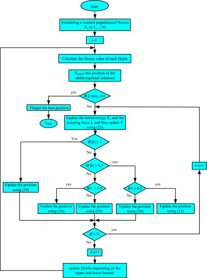
Flowchart of HHO optimization technique

4 Atom search optimization algorithm
The proposed ASO technique is considered as physics-based algorithm combined with swarm-based characteristics which is concerned mainly with finding the global optima, and thus, the ASO is designed with the help of analyzing the molecules dynamics and utilizing a heuristic algorithm which depends on the preserved population. In other words, it can be supposed that the operation of the proposed ASO relying on the search for the global optima though imitating the motion of the atoms which are controlled by interactivity and reservation forces [19, 29]. The construction of the ASO technique is very simple, while its performance is very competent. The ASO is used here to estimate with high degree of precision the PEMFC parameters, and its performance is compared with the HHO algorithm presented earlier and other previous techniques presented in the literature. Now, the total force acting on the ith atom can be calculated through adding all force components with different weights to each other which results in [30]:
where randj is an arbitrary number ranging from 0 to 1; Kbest is the first k atom which has the best fitness value in the subset of the atom population. Thus, in the proposed ASO, the exploration is enhanced during the first iterations through making each atom interact with the atoms which have better fitness values corresponding to their k neighbors. Then, the exploitation is enhanced at the late stages of iterations through making the atoms interact with few numbers of best fitted atoms. Thus, the K factor by which the interaction can be measured is expressed by
where N denotes the total number of atoms forming an atomic structure, t denotes the present iteration, and T is the total number of iterations. The interaction force due to the (L–J) potential is the most important variable which manages the motion of the atoms. The potential energy function is well analyzed and represented, and then, the force by which the atom j effects on the atom i can be expressed by [31]:
where η(t) is a function which is used to modify the depth and length of the attraction and repulsion regions; hij(t) is the ratio between the distance between two subsequent atoms rij, and the scaled distance between them σ(t).
where α denotes the depth weight. The dynamic behavior of function (36) with different \(\eta\) values and with \(h = \frac{\sigma }{r}\) from 0.9 to 2 is shown in Fig. 4. It can be noticed that the attraction is achieved for a range of h from 1.12 to 2 with the equilibrium line existing at h = 1.12. It can be also noticed that the attraction is increasing proportionally to h and reaches to its maximum value at h = 1.24, and then, the attraction starts to decrease again until it reaches zero at h = 2.

The behavior of the interaction force function with the scaled distance (h) under different depth values [29]
Based upon this, the ASO has to consider two limits: one for the repulsion with lower limit of h = 1.1 and one for the attraction with upper limit of h = 1.24 and accordingly, the value of h can be defined as follows:
where hmin and hmax describe the upper and lower limits of the distance (h), respectively, and determined by the following formula:
where \(k_{\text{best}}\) is the first k atom which has the best fitness value in the subset of the atom population, while g is a factor which is responsible for changing the algorithm behavior from exploration to exploitation and is represented by
The length dimension \(\sigma \left( t \right)\) is expressed by
where g0 and u denote the lower and upper limits, respectively. g(t) denotes a drift factor to give the algorithm the ability to transform from exploration to exploitation stage.
One of the most important factors which affect the atom motion is the geometric constraint. Each atom in the ASO is tied with the best element through a covalence bond, and thus, the best atom acts with different forces on the other atoms, and this action can be described by the following expression
where \(x_{\text{best}}\) is the location of the best element at the tth iteration, and \(b_{{i,{\text{best}}}}\) is a constant bond length between the best element and the specified ith atom. Thus, the developed constraint force can be evaluated by
where \(\gamma \left( t \right) = w{\text{e}}^{{\frac{ - 20t}{T}}}\) is the Lagrangian multiplier and w is a weighting factor.
After the determination of geometric constraint and interaction force, the acceleration of the ith atom in the population can be evaluated by [29, 30]:
where \(m_{i} \left( t \right)\) is the weight of the ith atom at a specified tth iteration. In addition, the value of \(m_{i} \left( t \right)\) can be determined by:
where \({\text{Fit}}_{i} \left( t \right)\) is the fitness value of the ith atom at the tth iteration, and \({\text{Fit}}_{\text{best}} \left( t \right)\) and \({\text{Fit}}_{\text{worst}} \left( t \right)\) are the best and worst fitness values of the atoms at the tth iteration which can be expressed by
To clarify more the ASO operation methodology, let’s express the position and velocity of an ith atom at iteration (t + 1)th by
where \(x_{i} \left( t \right)\) represents the position of the ith atom and \(a_{i}^{d} \left( t \right)\) refers to the atom acceleration and \(v_{i}^{d} \left( t \right)\) refers to the atom velocity. In conclusion, the sequence of implementation for the ASO algorithm can be summarized as follows:

5 Results
The simulation tests have been carried out to validate the proposed optimization algorithms (HHO and ASO). Both algorithms have been applied for estimating the parameters of PEM fuel cells. The two algorithms have been tested for estimating the parameters of three different modules of fuel cells, namely BCS 500W, SRR_12 modular and 250W stack. The data sheet parameters of these commercial PEMFC stacks are obtained from [6,7,8, 11, 12] and are presented in Table 1. Moreover, the estimated model parameters are ξ1, ξ2, ξ3, ξ4, β, RC and λ in PEMFC. The upper and lower limits of the unknown parameters for all case studies are given in [5, 7, 13, 14] and presented in Table 1 (last three columns in the right). The results of the two algorithms have been compared with each other and with those obtained using other techniques from the literature. Moreover, the optimized parameters using HHO and ASO methods have been used to estimate the performance and characteristics of the PEMFC at different operating conditions. Furthermore, the characteristics have been compared with the measured data of each module.
For the simulation, a dedicated software program for fuel cell parameter extraction problem is developed in MATLAB for HHO and ASO based upon their theories of operation which are described before. Simulations are performed using an Intel® core ™ i5-4210U CPU, 1.7 GHz, 8 GB RAM Laptop.
5.1 PEMFC of BCS 500W
To test and validate the proposed optimization algorithms, the proposed algorithms have been applied with the problem formulation PEM fuel cell of BCS 500W. The selected BCS 500W is studied because several studies have been introduced earlier for this purpose, but the majority have failed in achieving an accurate estimation for the parameters. The results of applying the HHO- and ASO-based algorithms to estimate the finest values of BCS 500W stack parameters are illustrated in Table 2. As shown from the table, the results gained by the HHO are better than those obtained by the ASO technique and also are better than the other methods from the literature. The convergence curves of the HHO and ASO are shown in Fig. 5, which reports that the HHO has the best convergence curve with respect to the speed of convergence and reaches the best minimum value of the objective function. From this figure, the HHO optimization algorithm reaches to a minimum value of 0.014879, while the ASO reaches to its minimum which is equal to 0.02661. It should be noted the small difference between the results of the two algorithms. Table 2 shows the comparison between the estimated parameters of the PEMFC model using HHO and ASO and other techniques.

Convergence curve of HHO and ASO optimization algorithms
To validate more the effectiveness of HHO optimization algorithm, the obtained results have been used to estimate the characteristics of the PEMFC by estimating the voltage and power curves versus the current. Furthermore, the estimated characteristics have been compared with the measured one as shown in Fig. 6. The figure shows a very good matching between the estimated and measured characteristics. Moreover, the characteristics of the PEMFC have been plotted at different operating conditions of pressure of PH2/PO2 of 1.000/0.2075 bar, 1.5/1.0 bar, 2.0/1.25 and 2.5/1.5 bar; and temperature of 303 K, 313 K, 323 K and 333 K as shown in Fig. 7.

The I/V and I/P curve characteristics of BCS 500W based on HHO optimization algorithm

Characteristics of BCS 500W with the variation of the temperature and pressure based on HHO optimization algorithm
5.2 SR-12PEM 500W
The second case of study is applied to estimate the model parameters of the SR-12PEM 500W. The parameters and data specification of the SR-12PEM 500W are listed in Table 1. The results of the estimated parameters are listed in Table 3. Also, Table 3 consists of a comparison between the ASO and HHO algorithms and with the obtained results by other researchers. From the table, the best solution has been reached by the ASO and equals 1.0803, while the best optimal value with the HHO is 1.0678. Moreover, the table shows that the other researchers with other optimization techniques could not reach the same solution. Furthermore, a comparison between ASO and HHO with respect to the convergence characteristics is shown in Fig. 8. The figure shows that the convergence speed of the HHO is better than that of the ASO.

Convergence curve of HHO and ASO optimization algorithms for the second case of study
The results of the characteristics of SR-12PEM 500W based on the estimated parameters using HHO and the experimental data are shown in Fig. 9. The figure shows that the obtained characteristics from the proposed HHO optimization algorithm introduce high matching degree with the experimental data. Moreover, due to the exploration characteristics of HHO, which is related to global search, the HHO keeps improving longer time than ASO. For more validating, the estimated model based on the HHO is used for plotting the characteristics at different operating conditions such as the variation of temperature and pressure as shown in Fig. 10.

The I/V and I/P curve characteristics of SR-12PEM 500W based on HHO optimization algorithm

Characteristics of SR-12PEM 500W with the variation of the temperature and pressure based on HHO optimization algorithm
5.3 250W stack
For more justification, the two algorithms of HHO and ASO have been applied for extracting the model parameters of the 250W stack. The data specifications of the 250W stack are listed in Table 1. The results of the estimated parameters are concluded in Table 4. From the table, it is revealed that the HHO algorithm has the best result with respect to reaching the minimum value of the objective function. The best optimal value of HHO is equal to 0.64577, while the best value with ASO equals 0.75884. Also, the table presents a comparison with other techniques from the literature. From the comparison, the optimal values of the objective function obtained by the HHO and ASO are better than the other techniques.
In order to analyze the convergence characteristics of the two algorithms, the convergence curves of the ASO and HHO algorithms via iterations are shown in Fig. 11. The figure shows that the HHO has a better convergence speed to solve the optimization problem compared with the ASO technique.

Convergence curve of HHO and ASO optimization algorithms for the second case of study
The validation of the results has been proved by plotting the voltage and power characteristics versus the current as shown in Fig. 12. From the figure, the precise matching between the estimated characteristics and the experimental data of the fuel cell can be easily investigated. Moreover, the characteristics of the module with the variation of the temperature and pressure are shown in Fig. 13.

The I/V and I/P curve characteristics of 250W stack based on HHO optimization algorithm

Characteristics of 250W stack with the variation of the temperature and pressure based on HHO optimization algorithm
6 Conclusion
A PEMFC is a nonlinear complicated dynamic system, which involves many interrelated parameters. This paper comprises the formulation of an optimization problem, which is devoted for optimal identification of the seven unknown parameters of the PEMFC. The HHO and ASO optimization techniques have been utilized for solving the optimization problem, while the fitness function is presented by the sum of square errors (SSE) between the actual and estimated models. The proposed methods introduced high performance with high matching degree with respect to the measured data of different fuel cell stacks. The HHO and ASO proved their effectiveness in reaching the optimal solution in a better way compared with the results in studies. From the comparison, it is concluded that the HHO is an accurate method which can precisely extract the parameters of the PEMFC with different cases of study. Therefore, it is recommended that the HHO algorithm can be implemented for solving sophisticated highly integrated optimization problems.
From the practical point of view, the estimated model can be used online with PEMFC for fault diagnosis and condition monitoring. Moreover, the estimated model also may be helpful with designing the real-time control PEMFC systems as well as system analysis. In the future work, the analysis of the parameter’s variations of the PEMFC model far from the standard operating conditions considering the presence of measuring noise should be performed.
References
Gaber HA (2017) Smart Energy Grid Engineering, 1st edn. Elsevier Inc, Amsterdam
Quaschning V (2016) Understanding Renewable Energy Systems, 2nd edn. Han ser. Verlag, Munich
Arshad A, Ali HM, Habib A, Bashir MA, Jabbal M, Yan Y (2019) Energy and exergy analysis of fuel cells: a review. Therm Sci Eng Progr 9:308–321
Sohani A, Naderi S, Torabi F (2019) Comprehensive comparative evaluation of different possible optimization scenarios for a polymer electrolyte membrane fuel cell. Energy Convers Manag 191(1):247–260
Cheng J, Zhang G (2014) Parameter fitting of PEMFC models based on adaptive differential evolution. Int J Electr Power Energy Syst 62:189–198
Sun Z, Wang N, Bi Y, Srinivasan D (2015) Parameter identification of PEMFC model based on hybrid adaptive differential evolution algorithm. Energy 90:1334–1341
Askarzadeh A, Rezazadeh A (2011) A grouping-based global harmony search algorithm for modeling of proton exchange membrane fuel cell. Int J Hydrogen Energy 36:5047–5053
Priya K, Babu TS, Balasubramanian K, Kumar KS, Rajasekar N (2015) A novel approach for fuel cell parameter estimation using simple genetic algorithm. Sustain Energy Technol Assess 12:46–52
Mo Z-J et al (2006) Parameter optimization for a PEMFC model with a hybrid genetic algorithm. Int J Energy Res 30(8):585–597
Zhang L, Wang N (2013) An adaptive RNA genetic algorithm for modeling of proton exchange membrane fuel cells. Int J Hydrogen Energy 38(1):219–228
Turgut OE, Coban MT (2016) Optimal proton exchange membrane fuel cell modelling based on hybrid Teaching Learning Based Optimization—differential evolution algorithm. Ain Shams Eng J 7(1):347–360. https://doi.org/10.1016/j.asej.2015.05.003
Ali M, El-Hameed MA, Farahat MA (2017) Effective parameters’ identification for polymer electrolyte membrane fuel cell models using grey wolf optimizer. Renew Energy 111:455–462
El-Fergany AA (2018) Electrical characterisation of proton exchange membrane fuel cells stack using grasshopper optimizer. IET Renew Power Gener 12(1):9–17
El-Fergany AA (2018) Extracting optimal parameters of PEM fuel cells using Salp Swarm Optimizer. Renew Energy 119:641–648
Rao Y, Shao Z, Ahangarnejad AH, Gholamalizadeh E, Sobhani B (2019) Shark smell optimizer applied to identify the optimal parameters of the proton exchange membrane fuel cell model. Energy Convers Manag 182:1–8
Shuhui X, Wang Y, Wang Z (2019) Parameter estimation of proton exchange membrane fuel cells using Eagle strategy based on JAYA algorithm and nelder-mead simplex method. Energy. https://doi.org/10.1016/j.energy.2019.02.106
Chen Y, Wang N (2019) Cuckoo search algorithm with explosion operator for modeling proton exchange membrane fuel cells. Int J Hydrogen Energy. https://doi.org/10.1016/j.ijhydene.2018.11.140
Liu Z, Zeng X, Ge Y, Shen J, Liu W (2017) Multi-objective optimization of operating conditions and channel structure for a proton exchange membrane fuel cell. Int J Heat Mass Transf 111:289–298
Zhao W, Wang L, Zhang Z (2019) Atom search optimization and its application to solve a hydrogeologic parameter estimation problem. Knowl Based Syst 163:283–304
Heidari AA, Mirjalili S, Faris H, Aljarah I, Mafarja M, Chen H (2019) Harris hawks optimization: Algorithm and applications. Future Gener Computer Syst 97:849–872. https://doi.org/10.1016/j.future.2019.02.028
El-Tamally HH, Sultan HM, Azzam M (2017) Control and operation of a solid oxide fuel-cell power plant in an isolated system. Adv Res J 2(3):10–20
Amphlett JC, Baumert RM, Mann RF, Peppley BA, Roberge PR (1995) Performance modeling of the Ballard mark IV solid polymer electrolyte fuel cell: empirical model development. J Electrochem Soc 142:9–15
Mo Z, Zhu X, Wei L, Cao G (2006) Parameter optimization for a PEMFC model with a hybrid genetic algorithm. Int J Energy Res 30:585–597
Mann RF, Amphlett JC, Hooper MAI, Jensen HM, Peppley BA, Roberge PR (2000) Development and application of a generalized steady-state electrochemical model for a PEM fuel cell. J Power Sour 86(1–2):173–180
Bao X, Jia H, Lang C (2019) A novel hybrid harris hawks optimization for color image multilevel thresholding segmentation. IEEE Access. https://doi.org/10.1109/ACCESS.2019.2921545
Abdel Aleem S, Zobaa A, Balci M, Ismael S (2019) Harmonic overloading minimization of frequency-dependent components in harmonics polluted distribution systems using Harris Hawks optimization algorithm. IEEE Access. https://doi.org/10.1109/access.2019.2930831
Viswanathan GM, Afanasyev V, Buldyrev S, Murphy E, Prince P, Stanley HE (1996) L´evy flight search patterns of wandering albatrosses. Nature 381:413
Sims DW, Southall EJ, Humphries NE, Hays GC, Bradshaw CJ, Pitchford JW, James A, Ahmed MZ, Brierley AS, Hindell MA et al (2008) Scaling laws of marine predator search behaviour. Nature 451:1098–1102
Zhao W, Wang L, Zhang Z (2019) A novel atom search optimization for dispersion coefficient estimation in groundwater. Future Gener Comput Syst 91:601–610
Gaing Z-L (2004) A particle swarm optimization approach for optimum design of PID controller in AVR system. IEEE Trans Energy Convers 19(2):384–391
Lennard-Jones JE (1924) On the determination of molecular fields. Proc R Soc Lond A Math Phys Eng Sci R Soc 106(738):463–477
Author information
Authors and Affiliations
Corresponding author
Ethics declarations
Conflict of interest
The authors declare no conflict of interest.
Additional information
Publisher's Note
Springer Nature remains neutral with regard to jurisdictional claims in published maps and institutional affiliations.
Rights and permissions
About this article

Cite this article
Mossa, M.A., Kamel, O.M., Sultan, H.M. et al. Parameter estimation of PEMFC model based on Harris Hawks’ optimization and atom search optimization algorithms. Neural Comput & Applic 33, 5555–5570 (2021). https://doi.org/10.1007/s00521-020-05333-4
Received:
Accepted:
Published:
Issue Date:
DOI: https://doi.org/10.1007/s00521-020-05333-4