
Abstract
The objective of this paper is to introduce a method for computing weights of attributes in a decision making problem under intuitionistic fuzzy environment. Many weight generation methods exist in the literature under intuitionistic fuzzy setting, but they have some limitations which can be pointed out as: the entropy measures used in entropy weight methods are invalid in many situations and also there are lots of entropy formulae for intuitionistic fuzzy sets, which will be better to use, and thus a confusion may arise; the other weight generation methods may lose some information since it needs to transform the intuitionistic fuzzy decision matrix into an interval-valued decision matrix. This conversion distorts experts original opinions. In this point of view, to overcome these demerits, we develop a weight generation method without changing the original decision information. The proposed method maximizes the average degree of satisfiability and minimizes the average degree of non-satisfiability of each alternative over a set of attributes, simultaneously. This leads to formulate a multi-objective programming problem (MOPP) to compute the final comprehensive value for each alternative. The scenario of an MOPP itself is subjective and can be modeled by fuzzy decision making problem due to the conflicting objectives and the way of human choice on conflict resolution. This problem is solved by using particle swarm optimization scheme, and the evaluation procedure is illustrated by means of a numerical example. This work has also justified the proposed approach by analyzing a comparative study.
1 Introduction
An important generalization of the classical fuzzy set theory is the theory of intuitionistic fuzzy set (IFS) introduced by Atanassov [1]. During the last decades, IFS theory has played a significant role for dealing with incomplete or inexact information present in real-world applications [2,3,4,5,6] including decision making problems. It is observed from the decision making problems that the weights of the attributes are determined usually beforehand. However, the proper assessment of attribute weights plays a vital role in multi-attribute decision making (MADM) problem as the variation of weights may affect on the final ranking order of the alternatives. In order to compute the weights of the attributes under intuitionistic fuzzy environment, several methods have been developed. For example, based on the technique for order of preference by similarity to ideal solution (TOPSIS) [7], a fractional programming model is developed by Li et al. [8] to determine attribute weights. By using TOPSIS method, Yue [9] presented a new method for group decision making problem with a weight determination process. On the basis of maximizing deviation method, Wei [10] introduced two optimization models to compute attribute weights where the information about attribute weights is completely unknown or partly known. In the same direction, Chou et al. [11] and Yeh and Chang [12] developed a weighting system of attributes under group decision-making conditions. Li [13] defined several linear programming models by using IFSs to determine attribute weights by maximizing the comprehensive values of alternatives over attributes. Lin et al. [14] provide a linear programming model which is much simpler than Li’s [13] method to generate weights of attributes. In terms of determining objective weights, one of the most representative approaches is the entropy method [15]. Ye [16] established a weight generation method where attribute weights are completely unknown based on weighted correlation coefficient measure with entropy. Wu and Zhang [17] introduced a linear programming model to determine the optimal weight of criteria based on intuitionistic fuzzy weighted entropy. By using gray relational analysis (GRA), Wei [18, 19] computed weights of criteria in a decision making problem.
Although numerous weight computation methods have been developed under intuitionistic fuzzy environment, they have some limitations which can be listed as follows: the entropy measure used in entropy weight methods [15,16,17] is invalid in many situations, and also there are lots of entropy formulae for IFSs, which will be better to use and thus should be improved; the other weight generation methods [13, 14] may loss some information since these processes need to be transformed the intuitionistic fuzzy decision matrix into an interval-valued decision matrix. This conversion distorts experts original opinions. In this point of view, without changing the original decision information, we have developed a weight generation method by maximizing the average degree of satisfiability and minimizing the average degree of non-satisfiability of each alternative over a set of attributes, simultaneously in the form of multi-objective programming problem (MOPP), which is nonlinear. A global optimization process is required to solve this nonlinear problem. In this work, we employ a recently developed optimization technique, namely particle swarm optimization (PSO) to find the compromise solution of MOPP under the intuitionistic fuzzy environment. Then, an approach to MADM problem in which the ratings of alternatives on the basis of attributes are expressed as IFSs is developed with incomplete attribute weights information.
The paper is organized as follows: in Sect. 2, primary discussions of the various useful ideas including MOPP, PSO, penalty function and IFSs are provided in brief. The proposed approach to determine attribute weights under intuitionistic fuzzy environment is presented in Sect. 3. In Sect. 4, a numerical example is studied for clarifying our proposed method and the comparison analysis is also conducted. Finally, a concrete conclusion is drawn in Sect. 5.
2 Preliminary
In this section, we carry out brief introductions to MOPP, PSO, penalty function and IFSs that will be required for our subsequent developments. We start by recalling the concepts of MOPP.
2.1 Multi-objective programming problem
An MOPP is a design process that optimizes a vector of objective functions in a systematic way by considering all the objective functions simultaneously. A general MOPP can be defined as follows:
where \(f_{1}(x),f_{2}(x),\ldots ,f_{n}(x)\) are n individual objective functions, \(x \in \mathbb {R}^{n}\) is a vector of decision variables, \(A_{i} \in \mathbb {R}^{m\times n}\) and \(b_{i} \in \mathbb {R} (i=1,2,\ldots ,m)\). The MOPP is designed here to find the decision variables x which optimizes a vector of objective functions \(f(x)=((f_{1}(x),f_{2}(x),\ldots ,f_{n}(x))\) in the feasible decision space. Due to the conflicting nature of objective functions, it is not necessary that MOPP has an optimal solution that maximizes/minimizes all the objective functions simultaneously. This is the scenario of tradeoff between objective functions. This leads us to find the best compromise solution, called Pareto optimal solution [20]. Generally, by a Pareto optimal solution, we mean a solution for which improvement of one objective can be achieved only at the expense of another [21]. Mathematically, it can be represented as follows:
Definition 1
[20] A solution vector \(x^{*} \in X\) is said to be a Pareto optimal to MOPP if there does not exist any \(x \in X\) such that \(f_{i}(x) \ge f_{i}(x^{*})\), for all i and \(f_{i}(x) > f_{i}(x^{*})\) for at least one \(i=1,2,\ldots ,m\).
In general, the solution procedure of an MOPP is classified into following two categories: classical methods and evolutionary methods. From last few decades, many classical methods [20], such as weighted sum method, \(\epsilon \)-constraint method, value function method, goal programming, interactive method, have been used to solve an MOPP. Most of the classical methods are not efficient for solving an MOPP due to get stuck at a suboptimal solution. To overcome this situation, over the last decade, evolutionary algorithms, such as genetic algorithm (GA) [22, 23], PSO [24,25,26], ant colony optimization [27], have been extensively used in the field of science and engineering disciplines.
In order to cope with imprecise information present in real-life problems, the study of MOPP is started in fuzzy environment. Fuzzy MOPPs are studied by Bellman and Zadeh [28], Zimmermann [29], Sakwa and Yano [30] and many others. Cheng et al. [31] solved fuzzy multi-objective linear programming problem by utilizing deviation method and weighted max–min method. By extending the concept of TOPSIS approach, a methodology [32] is developed for solving multiple objective decision making problems. Recently, Deep et al. [33] proposed an interactive method by using GA for solving MOPP in fuzzy environment. GA is also used by Sakwa and Yauchi [34] for the same purpose. A more comprehensive detail of evolutionary algorithms for MOPP can be found in [20].
2.2 Particle swarm optimization
In order to solve a nonlinear optimization problem, PSO is one of the most successful and widely used algorithms. PSO, introduced by Kennedy and Eberhart [24], is a population-based stochastic global optimization method which is inspired by bird flocking, fish schooling and swarming theory. PSO is developed on the basis of communication and interaction, i.e., information exchange between members, called ‘particles,’ of the population, called ‘swarm.’ During movement, each particle adjusts its best position (local best) according to its own previous best position and the best position attained by any neighbor particles (global best). PSO starts with a swarm of particles whose positions are initial solutions and the velocities are randomly initialized in the search space. Based on the local best and global best information, particles update their positions and velocities.
In each iteration, the velocity and position of the particle are updated according to the following equations.
where i(=1,2,...,n) represents the number of particles in population and n is the population size; \(v_{i}(k+1)\) is the velocity of ith particle in the \((k+1)\)th iteration; \(\xi (k)\) is the constriction factor which controls and constricts velocities of particles; \(\omega \) is the inertia weight; \(r_{i1}\) and \(r_{i2}\) are random numbers generated from a uniform distribution in the interval [0,1]; \(c_{1}\) and \(c_{2}\), called ‘cognitive’ and ‘social’ parameter, respectively, are positive constants; \(x_{i}(k+1)\) is the position of ith particle in the \((k+1)\)th iteration. So, at each generation, Eq. (2) is performed as a new velocity, whereas Eq. (3) represents the new position of particles.
The performance of each particle is evaluated according to fitness function which is problem dependent. Generally, in optimization problem, the objective function is treated as the fitness function.
From the applicability point of view, in this work, we utilize PSO as a tool to solve the nonlinear constrained optimization problem. The constrained optimization problem is changed into the equivalent unconstrained problem by using penalty function approach which is discussed in the next subsection. Now, a brief description of a pseudo code of PSO algorithm is given below.
Algorithm: Pseudo code of particle swarm optimization (PSO)
Step-1: Select objective function: \(f(x); x=(x_{1}, x_{2},\ldots ,x_{n})\) as a fitness function |
Step-2: Set iteration number \(k = 0\) |
Step-3: Initialize particle position and velocity for each particle |
Step-4: Initialize the particle’s best known position to its initial position, i.e., \(x_{i}^{l}(k)=x_{i}(k)\) |
Step-5: Repeat |
Step-6: Set iteration number \(k = k+1\) |
Step-7: Update the best known position \(x_{i}^{l}(k)\) of each particle and the swarm’s best known position \(x_{i}^{g}(k)\) |
Step-8: Evaluate particle velocity and position according to Eqs. (2) and (3) |
Step-9: Continue until termination criterion met |
2.3 Penalty function
Constrained optimization problems have two types of solutions, one is feasible which satisfies all the given constraints, whereas another one is infeasible which violates at least one of them. In order to solve a constrained optimization problem, one of the successful approaches is to use of penalty function [35]. In the penalty function approach, constrained optimization problem is reduced to unconstrained optimization problem by introducing a penalty function and making a single-objective function. The idea behind this method is that penalty function assigns zero penalty if the point is feasible one and it assigns positive penalty if the point is infeasible. The penalty function can be defined as
Definition 2
[36] A function \(P:\mathbb {R}^{n}\rightarrow \mathbb {R}\) is called a penalty function if P satisfies following properties:
-
1.
P(x) is continuous;
-
2.
\(P(x)\ge 0\quad \forall x \in \mathbb {R}^n\);
-
3.
\(P(x)= 0\,\, \forall \) feasible x;
-
4.
\(\lim P(x)= \infty ~\) if \(|x|\rightarrow \infty \).
Now, the constrained problem (1) can be transformed to unconstrained optimization problem by using a penalty function as
where k is the current iteration number, \(\alpha (k)\) is the penalty parameter and \(\alpha (k)>0, \alpha (k)\le \alpha (k+1) \quad \forall k\), in practice \(\{\alpha _{k}\}\) is taken as \(\{\alpha _{1}=1, \alpha _{2}=10,\alpha _{3}=100,\alpha _{4}=1000,\ldots . \}\) and penalty function P(x) is defined as
where \(q_{i}(x)=\max \{0,g_{i}(x)\}\), \(g_{i}(x)=A_{i}x-b_{i}\) and r is the power of a penalty function. In general r is taken as \(r=1\) or \(r=2\).
2.4 Intuitionistic fuzzy set
An important generalization of classical fuzzy set theory [37] is the theory of IFS [1] which comprehensively portrays the uncertainty of human beings when providing expert’s opinion over the objects. The definition of IFS is given in below.
An IFS a in the universe X can be expressed as a set of ordered triplets, \(a=\{(x,\mu _{a}(x),\nu _{a}(x)):x\in X\}\), where \(\mu _{a}: X\rightarrow [0,1]\) is the degree of belongingness and \(\nu _{a}: X\rightarrow [0,1]\) is the degree of non-belongingness of x in a. They satisfy the relation \(0\le \mu _{a}(x)+\nu _{a}(x)\le 1\)\( \forall x\in X\). Each fuzzy set is a special case of IFS, and it can be represented as \(a=\{(x,\mu _{a}(x),1-\mu _{a}(x)):x\in X\}\). The quantity \(\pi _{a}(x)=1-\mu _{a}(x)-\nu _{a}(x)\) is called the degree of hesitation (indeterminacy) of x in a. When \(\pi _{a}(x)=0\)\(\forall x\in X\), IFS becomes fuzzy set.
For the sake of simplicity now onwards, we will write an IFS a as \(a=(\mu _{a},\nu _{a})\) throughout the paper.
3 An approach to MADM problem with incomplete attribute weight information
In this section, we consider a framework for MADM problem with incomplete attribute weight information where ratings of alternatives over attributes are given as IFSs.
3.1 Problem formulation
Now, a MADM problem with IFSs is presented in which information of attribute weights is partly known. A multi-attribute single-expert decision process is designed with n attributes \(C=\{C_{1},C_{2},\ldots ,C_{n}\}\) to evaluate m number of alternatives \(A=\{A_{1},A_{2},\ldots ,A_{m}\}\). Assume that \(w=(w_{1},w_{2},\ldots ,w_{n})^{T}\) be the weight vector of attributes, where \(w_{j} \in [0,1]\), \(j=1,2,\ldots ,n\) which are partly known and \( \sum _{j=1}^{n}w_{j}=1\).
Suppose, IFS \(a_{ij}=(\mu _{a_{ij}}, \nu _{a_{ij}})\) denotes the expert’s assessment corresponding to \(j^{th}\) attribute \(C_{j}(j=1,2,\ldots ,n)\) to evaluate \(i^{th}\) alternative \(A_{i}(i=1,2,\ldots ,m)\).
The MADM process can be described in the following way:
- Step 1: :
-
Construction of decision matrix
A MADM problem with IFSs can be represented concisely in a matrix form as follows:

where each \(a_{ij}\) is IFS \(a_{ij}=(\mu _{a_{ij}}, \nu _{a_{ij}})\).
- Step 2: :
-
Computation of comprehensive values of each alternative
The comprehensive values for each alternative are calculated by weighted intuitionistic fuzzy arithmetic mean operator [38]. Let \(Z_{i}\) be the comprehensive values corresponding to the alternative \(A_{i}(i=1,2,\ldots ,m)\), with
$$\begin{aligned} Z_{i}=(P_{i}, Q_{i})=\Big (1- \prod _{j=1}^{n}(1-\mu _{a_{ij}}^{w_{j}}), \prod _{j=1}^{n}\nu _{a_{ij}}^{w_{j}}\Big ) \end{aligned}$$(6)where \(P_{i}=1- \prod\nolimits _{j=1}^{n}(1-\mu _{a_{ij}}^{w_{j}})\) represents the membership degree of the comprehensive value (called the degree of satisfiability) and \(Q_{i}= \prod\nolimits _{j=1}^{n}\nu _{a_{ij}}^{w_{j}}\) represents the non-membership degree of the comprehensive value (called the degree of non-satisfiability) of the alternative \(A_{i}\).

3.2 Estimation of attribute weights by constructing MOPP
In this subsection, an attribute weight determination method in a decision making process is developed by maximizing the degree of satisfiability and minimizing the degree of non-satisfiability. The methodology consists of following two steps:
- Step 3: :
-
MOPP formulation
Sometimes, it may happen that decision maker only possesses partial information about attribute weights due to the increasing complexity of real-world decision situations. Based on the weighted intuitionistic fuzzy arithmetic values, we select the optimal weight vector \(w = (w_{j})^{T}(j=1,2,\ldots n)\) to maximize membership degree of the comprehensive values and minimize the non-membership degree of the comprehensive values of alternatives for all the attributes. For each alternative \(A_{i}(i=1,2,\ldots ,m)\), the final comprehensive value can be computed through the following multi-objective programming model (Model-1):
$$\begin{aligned} \hbox {Model}-1: \alpha _{i}&= \max _{w} P_{i}=1- \prod _{j=1}^{n}(1-\mu _{a_{ij}}^{w_{j}})\\ \beta _{i}&= \min _{w} Q_{i}= \prod _{j=1}^{n}\nu _{a_{ij}}^{w_{j}}\\ \hbox {subject to }&\quad w\in H,\\& \sum _{j=1}^{n}w_{j}=1,\\&w_{j}\ge 0,\quad j=1,2,\ldots ,n \end{aligned}$$where H is the set of incomplete information about attribute weights. The objective function \( \max _{w} P_{i}\) implicates that average membership values for each alternative are maximized, i.e., the degree of satisfiability of each alternative over a set of attributes is maximized. The objective function \( \min _{w} Q_{i}\) represents that average non-membership values for each alternative are minimized, i.e., the degree of non-satisfiability of each alternative over a set of attributes is minimized.
- Step 4: :
-
Fuzzy MOPP formulation
In the MOPP scenario, it is worth noticing that multiple objectives conflict with each other and thus, in multi-objective optimization there is no optimal solution for all the objectives. Thus, the notion of Pareto optimality [20] or efficiency has been introduced in MOPP instead of the optimality concept for single-objective optimization. Decisions with Pareto optimality or efficiency cannot be uniquely determined. However, for practical applications, one solution needs to be selected, which will satisfy the different goals to some extent. Such a solution is called best compromise solution. In this aspect, due to the imprecision or fuzziness inherent in human judgments, it is quite natural to assume that the decision maker may have a fuzzy goal for each of the objective functions. The fuzzy goals of the decision maker for each of the objective functions can be incorporated in the problem formulation of MOPP via fuzzy sets, which are characterized by membership functions [39].
In order to construct the membership function of each objective, first we solve the following two crisp single-objective optimization problems (one is maximization and one is minimization) separately. Therefore, for each objective \(P_{i}~(i=1,2,\ldots ,m)\), the following two single-objective optimization problems are solved:
to get two individual values \(\alpha _{i}^{L}\) (minimum value of the objective function \(P_{i}\)) and \(\alpha _{i}^{U}\) (maximum value of the objective function \(P_{i}\)) for every objective function \(P_{i}\). In the same way, for each objective \(Q_{i}~(i=1,2,\ldots ,m)\), the following two single-objective optimization problems are solved:
to generate two individual values \(\beta _{i}^{L}\) (minimum value of the objective function \(Q_{i}\)) and \(\beta _{i}^{U}\) (maximum value of the objective function \(Q_{i}\)) for every objective function \(Q_{i}\).
In the present study, for easy understanding and obvious computational advantage, simple linear membership functions \(\mu _{P_{i}}\) and \(\mu _{Q_{i}}~(i=1,2,\ldots ,m)\) corresponding to the objective functions \(P_{i}\) and \(Q_{i}~(i=1,2,\ldots ,m)\), respectively, are introduced to represent the goal of each objective function as follows:
and

Membership function for the min type objective functions

Membership function for the min type objective functions
The membership functions \(\mu _{P_{i}}(w)\) (Fig. 1) and \(\mu _{Q_{i}}(w)\) (Fig. 2) represent the degree of satisfactions of the decision maker corresponding to the objective functions \(P_{i}\) and \(Q_{i}\), respectively, as a value between zero and one. Having elicited the membership functions \(\mu _{P_{i}}(w)\) and \(\mu _{Q_{i}}(w)~(i=1,2,\ldots ,m)\) for each of the objective functions \(P_{i}\) and \(Q_{i}~(i=1,2,\ldots ,m)\), respectively, through the interaction of decision maker, the MOPP (Model 1) can be transformed into the fuzzy MOPP defined by
One of the important steps in fuzzy MOPP is the aggregation of membership values of the objective functions to reduce it into a single-objective optimization problem. The aforementioned fuzzy MOPP can be reduced into the single-objective optimization problem based on the concept of aggregation operator in the following way:
where f represents an aggregation function. It is to be noted that the value of \(f(\mu _{P_{1}}(w),\mu _{P_{2}}(w),\ldots ,\mu _{P_{m}}(w), \mu _{Q_{1}}(w),\mu _{Q_{2}}(w),\ldots ,\mu _{Q_{m}}(w))\) can be interpreted as the overall degree of satisfaction of decision makers’ fuzzy goals. However, one may use arithmetic mean, geometric mean, minimum operator, product operator as an aggregation function f. To aggregate the objective functions, among the several choices, weighted arithmetic mean [40] and minimum operator [31] are often used in the literature. Inspired by the work [28, 29, 31], we use minimum operator as an aggregation function which may be given as follows:
Hence, eliciting the choice of aggregation function f, the aforementioned optimization problem (Model 1) turns into the following single-objective nonlinear optimization problem (Model 2) defined as follows:
where \(\lambda = \min _{i=1,..,m} \{\mu _{P_{i}}(w), \mu _{Q_{i}}(w)\}\) is the satisfactory level.
As Model-2 is nonlinear in nature with multiple variables, it is really a difficult task to find out the gradient vector and thus it requires some effective methods and algorithms for finding the global solution. One of the most useful processes that exists in the literature to find out the global solution of the nonlinear optimization problem is the evolutionary algorithmic (EA) approach [41]. The advantage of this EA technique is that it does not require any kind of pre-assumptions, such as continuity, differentiability of objective functions [39].
In the present work, we employ a recently developed EA technique, namely PSO [24], to solve Model-2. In order to solve Model-2, first we convert the constrained optimization problem into unconstrained optimization problem by a penalty function. The PSO is implemented by utilizing the algorithm in Matlab R2013a. The solutions of the above optimization problem (Model-2) provide weights of the criteria. If \((w^{*}, \lambda ^{*})\) is a global optimal solution of Model-2, then it implies that the maximum degree of overall satisfaction \(\lambda ^{*}\) is achieved for the solution \(w^{*}\).
3.3 Computation of the final aggregated values for each alternative and ranking of the alternatives
Final weighted aggregated values of alternatives \(A_{i}\) are determined by utilizing weights of the attributes derived from the above optimization problem and the weighted intuitionistic fuzzy arithmetic mean operator [38] (Eq. 6).
3.4 Ranking of the alternatives
Finally, ranking of all the alternatives is done according to the non-increasing order of the score function [42] defined as follows:
4 Numerical example
In this section, a numerical example is considered to illustrate the feasibility and effectiveness of the proposed weight generation method of attributes in a decision making problem under intuitionistic fuzzy environment.
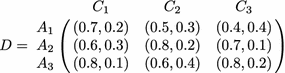
An investment company wants to invest money in the best possible option (adapted from [2]). The three possible alternatives to invest money are: (1) \(A_{1}\) is a car company; (2) \(A_{2}\) is a food company; (3) \(A_{3}\) is a computer company. The investment company must take a decision according to the following three attributes: \(C_{1}\): the risk analysis; \(C_{2}\): the growth analysis; \(C_{3}\): the environmental impact analysis. The ratings of the alternatives over the attributes are evaluated by utilizing IFSs. Now, the weights of attributes and ordering of the alternatives are computed as follows.
- Step 1: :
-
Construction of decision matrix
Ratings of the alternatives over the attributes are given in the following matrix:
- Step 2: :
-
Computation of comprehensive values of each alternative
The comprehensive value of each alternative is calculated by weighted intuitionistic fuzzy arithmetic mean operator. Let \(Z_{1}, Z_{2}\) and \(Z_{3}\) be the comprehensive values corresponding to the alternatives \(A_{1}, A_{2}\) and \(A_{3}\), respectively, and
$$\begin{aligned} Z_{1}&= (P_{1},Q_{1})=(1-0.3^{w_{1}}0.5^{w_{2}}0.6^{w_{3}}, 0.2^{w_{1}}0.3^{w_{2}}0.4^{w_{3}})\\ Z_{2}&= (P_{2},Q_{2})=(1-0.4^{w_{1}}0.2^{w_{2}}0.3^{w_{3}}, 0.3^{w_{1}}0.2^{w_{2}}0.1^{w_{3}})\\ Z_{3}&= (P_{3},Q_{3})=(1-0.2^{w_{1}}0.4^{w_{2}}0.2^{w_{3}}, 0.1^{w_{1}}0.4^{w_{2}}0.2^{w_{3}}) \end{aligned}$$where \(w_{1}, w_{2}\) and \(w_{3}\) are the weights of the attributes \(C_{1}, C_{2}\) and \(C_{3}\), respectively. Attribute weights \(w_{1}, w_{2}\) and \(w_{3}\) are computed as follows:
- Step 3: :
-
MOPP formulation
Assume that the information about attribute weights \(w_{j}\) is partly known and the partial weight information is given as follows:
$$\begin{aligned} H=\{0.25 \le w_{1}\le 0.75, 0.15 \le w_{2} \le 0.6, 0.2 \le w_{3} \le 0.35\}. \end{aligned}$$By using Model-1, described in Sect. 3.2, we have,
$$\begin{aligned} \max P_{1}&= 1-0.3^{w_{1}}0.5^{w_{2}}0.6^{w_{3}}\\ \max P_{2}&= 1-0.4^{w_{1}}0.2^{w_{2}}0.3^{w_{3}}\\ \max P_{3}&= 1-0.2^{w_{1}}0.4^{w_{2}}0.2^{w_{3}}\\ \min Q_{1}&= 0.2^{w_{1}}0.3^{w_{2}}0.4^{w_{3}}\\ \min Q_{2}&= 0.3^{w_{1}}0.2^{w_{2}}0.1^{w_{3}}\\ \min Q_{3}&= 0.1^{w_{1}}0.4^{w_{2}}0.2^{w_{3}}\\ \\ \hbox {subject to}&\quad 0.25 \le w_{1} \le 0.75,\\&0.15 \le w_{2} \le 0.60,\\&0.20 \le w_{3} \le 0.35,\\&w_{1}+w_{2}+w_{3}=1,\\&w_{j}\ge 0, j=1,2,3 \end{aligned}$$ - Step 4: :
-
Fuzzy MOPP formulation
To get a maximum value and a minimum value of each objective function, we have solved \(2\times 6=12\) crisp single-objective optimization problems (one maximization and one minimization for each single optimization problem) by PSO scheme and the values are shown in Table 1.

The membership functions corresponding to objective functions, for describing the fuzziness involved in each objective, are defined as follows:
So, by utilizing Eqs. (10)–(15) and Model-2, the single-objective optimization problem can be formulated as:
After simplification, we will get,
This is a nonlinear optimization problem. By using PSO scheme we get,
- Step 5: :
-
Computation of the final aggregated values for each alternative.
By utilizing the weight values of the attributes and the weighted intuitionistic fuzzy arithmetic mean operator [38], the final aggregated values of the alternatives \(A_{i}(i=1,2,3)\) are
$$\begin{aligned} Z_{1}=(0.6194,0.2659), Z_{2}=(0.7042,0.2076), Z_{3}=(0.7451,0.1874) \end{aligned}$$ - Step 6: :
-
Ranking of the alternatives.
By utilizing Eq. (9), the score values of alternatives are computed as follows:
$$\begin{aligned} S(Z_{1})=0.3535, S(Z_{2})=0.4966, S(Z_{3})=0.5577 \end{aligned}$$Ranking order is: \(A_{3}>A_{2}>A_{1}\), i.e., the most desirable alternative is \(A_{3}\).
4.1 Comparison analysis
4.1.1 Comparison analysis with GA
To further illustrate the effectiveness of the proposed method, we solve the above investment option selection problem (described in Sect. 4) by using GA [20]. In order to compare performance of the proposed weight generation method, we employ GA to solve above optimization problems and then compute the ranking of alternatives by following the same steps as in the proposed decision making process. Based on the alternatives’ final performances, ranking order of the alternatives in each of the cases is presented in Table 2.
It is observed from Table 2 that the ranking order of attribute weights as well as the ranking order of alternatives, obtained by using GA and PSO are same.
4.1.2 Comparison analysis with existing weight generation methods
In this section, we compare the proposed weight computation method with other existing approaches, such as Li’s process [13], Lin et al. process [14], GRA process [18], knowledge-based process [2] and maximizing deviation process [10] by using the investment option selection problem described in Sect. 4. The above MADM example is solved by the aforementioned approaches, and the results are shown in Table 3.
As can be seen from Table 3, the ranking order of attribute weights and the ranking order of the alternatives obtained by different methods are same as it did by the proposed method and all of them identify \(A_{3}\) as the most desirable company to invest money. The foregoing discussion ensures that in the case of weight generation in decision making problem, the proposed method works well. This observation verifies the effectiveness of the proposed method. Moreover, the ranking results obtained by different existing methods and proposed methods are depicted in Fig. 3.

Ranking results by different approaches in the IFS context when weight information is partly known
Hence, from the aspects of theoretical analysis and particular application viewpoint it is clear that the proposed weight generation method is able to cope with the situations where attribute weight information is partly known.
5 Conclusion
This study has presented a weight determination method in a decision making process with intuitionistic fuzzy setting. The weight generation methods that exist in the literature under intuitionistic fuzzy environment have some shortcomings: some weight generation methods are invalid in many situations and thus should be improved; the other weight generation methods may lose some information due to that they need to be transformed the intuitionistic fuzzy decision matrix into an interval-valued decision matrix. Under these circumstances, without changing the original decision information, we have developed a weight determination method by maximizing the average degree of satisfiability and minimizing the average degree of non-satisfiability of each alternative over a set of attributes, simultaneously. We have formulated an MOPP to compute the final comprehensive values for each alternative, and this MOPP is modeled by fuzzy decision making problem and solved by using PSO technique. Finally, we have considered a numerical example to describe effectiveness and applicability of the proposed weight generation method.
Although the proposed weight generation approach is illustrated by a selection problem of an investment company, it can also be applied to any other areas of decision problems where uncertainty and hesitation are involved in the evaluation process. This will be the topic of our future research work.
References
Atanassov KT (1986) Intuitionistic fuzzy sets. Fuzzy sets Syst 20(1):87–96
Das S, Dutta B, Guha D (2015) Weight computation of criteria in a decision-making problem by knowledge measure with intuitionistic fuzzy set and interval-valued intuitionistic fuzzy set. Soft Comput. doi:10.1007/s00500-015-1813-3
Wei G (2010) Some induced geometric aggregation operators with intuitionistic fuzzy information and their application to group decision making. Appl Soft Comput 10(2):423–431
Wei G, Zhao X (2011) Minimum deviation models for multiple attribute decision making in intuitionistic fuzzy setting. Int J Comput Intell Syst 4(2):174–183
Wei G, Wang H-J, Lin R, Zhao X (2011) Grey relational analysis method for intuitionistic fuzzy multiple attribute decision making with preference information on alternatives. Int J Comput Intell Syst 4(2):164–173
Nguyen H (2015) A new knowledge-based measure for intuitionistic fuzzy sets and its application in multiple attribute group decision making. Expert Syst Appl 42(22):8766–8774
Tzeng G-H, Huang J-J (2011) Multiple attribute decision making: methods and applications. CRC Press, Boca Raton
Li D-F, Wang Y-C, Liu S, Shan F (2009) Fractional programming methodology for multi-attribute group decision-making using ifs. Appl Soft Comput 9(1):219–225
Yue Z (2011) A method for group decision-making based on determining weights of decision makers using topsis. Appl Math Modelling 35(4):1926–1936
Wei G-W (2008) Maximizing deviation method for multiple attribute decision making in intuitionistic fuzzy setting. Knowl Based Syst 21(8):833–836
Chou S-Y, Chang Y-H, Shen C-Y (2008) A fuzzy simple additive weighting system under group decision-making for facility location selection with objective/subjective attributes. Eur J Oper Res 189(1):132–145
Yeh C-H, Chang Y-H (2009) Modeling subjective evaluation for fuzzy group multicriteria decision making. Eur J Oper Res 194(2):464–473
Li D-F (2005) Multiattribute decision making models and methods using intuitionistic fuzzy sets. J Comput Syst Sci 70(1):73–85
Lin L, Yuan X-H, Xia Z-Q (2007) Multicriteria fuzzy decision-making methods based on intuitionistic fuzzy sets. J Comput Syst Sci 73(1):84–88
Xia M, Xu Z (2012) Entropy/cross entropy-based group decision making under intuitionistic fuzzy environment. Inf Fus 13(1):31–47
Ye J (2010) Fuzzy decision-making method based on the weighted correlation coefficient under intuitionistic fuzzy environment. Eur J Oper Res 205(1):202–204
Wu J-Z, Zhang Q (2011) Multicriteria decision making method based on intuitionistic fuzzy weighted entropy. Expert Syst Appl 38(1):916–922
Wei G-W (2010) GRA method for multiple attribute decision making with incomplete weight information in intuitionistic fuzzy setting. Knowl Based Syst 23(3):243–247
Wei G-W (2011) Gray relational analysis method for intuitionistic fuzzy multiple attribute decision making. Expert Syst Appl 38(9):11671–11677
Deb K (2001) Multi-objective optimization using evolutionary algorithms, vol 16. John Wiley & Sons, Hoboken
Sakawa M, Yano H (1985) An interactive fuzzy satisficing method using augmented minimax problems and its application to environmental systems. IEEE Trans Syst Man Cybern 6:720–729
Goldberg DE, Korb B, Deb K (1989) Messy genetic algorithms: motivation, analysis, and first results. Complex Syst 3(5):493–530
Ding S, Xu L, Su C, Jin F (2012) An optimizing method of RBF neural network based on genetic algorithm. Neural Comput Appl 21(2):333–336
Kennedy J (2010) Particle swarm optimization. In: Sammut C, Webb GI (eds) Encyclopedia of machine learning. Springer, Berlin, pp 760–766
Marini F, Walczak B (2015) Particle swarm optimization (PSO). A tutorial. Chemom Intell Lab Syst 149:153–165
Hamza MF, Hwa HJ, Choudhury IA (2017) Recent advances on the use of meta-heuristic optimization algorithms to optimize the type-2 fuzzy logic systems in intelligent control. Neural Comput Appl. doi:10.1007/s00521-015-2111-9
Dorigo M, Caro G, Gambardella L (1999) Ant algorithms for discrete optimization. Artif Life 5(2):137–172
Bellman RE, Zadeh LA (1970) Decision-making in a fuzzy environment. Manag Sci 17(4):B-141
Zimmermann H-J (1978) Fuzzy programming and linear programming with several objective functions. Fuzzy Sets Syst 1(1):45–55
Sakawa M, Yano H (1988) An interactive fuzzy satisficing method for multiobjective linear fractional programming problems. Fuzzy Sets Syst 28(2):129–144
Cheng H, Huang W, Zhou Q, Cai J (2013) Solving fuzzy multi-objective linear programming problems using deviation degree measures and weighted max–min method. Appl Math Modelling 37(10):6855–6869
Baky IA, Abo-Sinna MA (2013) Topsis for bi-level modm problems. Appl Math Modelling 37(3):1004–1015
Deep K, Singh KP, Kansal M, Mohan C (2011) An interactive method using genetic algorithm for multi-objective optimization problems modeled in fuzzy environment. Expert Syst Appl 38(3):1659–1667
Sakawa M, Yauchi K (2001) An interactive fuzzy satisficing method for multiobjective nonconvex programming problems with fuzzy numbers through coevolutionary genetic algorithms. IEEE Trans Syst Man Cybern Part B Cybern 31(3):459–467
Chandra S, Jayadeva MA (2009) Numerical optimization with applications. Alpha Science International, Oxford
Berhe HW (2012) Penalty function methods using matrix laboratory (MATLAB). Afr J Math Comput Sci Res 5(13):209–246
Zadeh LA (1965) Fuzzy sets. Inf Control 8(3):338–353
Xu Z (2007) Intuitionistic fuzzy aggregation operators. IEEE Trans Fuzzy Syst 15(6):1179–1187
Chakraborty D, Guha D, Dutta B (2016) Multi-objective optimization problem under fuzzy rule constraints using particle swarm optimization. Soft Comput. doi:10.1007/s00500-015-1639-z
Li L, Lai KK (2000) A fuzzy approach to the multiobjective transportation problem. Comput Oper Res 27(1):43–57
Eiben AE, Smith JE (2003) Introduction to evolutionary computing. Springer, Berlin
Chen S-M, Tan J-M (1994) Handling multicriteria fuzzy decision-making problems based on vague set theory. Fuzzy Sets Syst 67(2):163–172
Acknowledgements
The first author receives the research grant from the Ministry of Human Resource Development, Government of India. The second author acknowledges the support of Grant ECR/2016/001908.
Author information
Authors and Affiliations
Corresponding author
Ethics declarations
Conflict of interest
The authors declare that they have no other conflict of interest.
Rights and permissions
About this article

Cite this article
Das, S., Guha, D. Attribute weight computation in a decision making problem by particle swarm optimization. Neural Comput & Applic 31, 2495–2505 (2019). https://doi.org/10.1007/s00521-017-3209-z
Received:
Accepted:
Published:
Issue Date:
DOI: https://doi.org/10.1007/s00521-017-3209-z