A hybrid grasshopper and new cat swarm optimization algorithm for feature selection and optimization of multi-layer perceptron

Abstract

The classification accuracy of a multi-layer perceptron (MLP) depends on the selection of relevant features from the data set, its architecture, connection weights and the transfer functions. Generating an optimal value of all these parameters together is a complex task. Metaheuristic algorithms are popular choice among researchers to solve complex optimization problems. This paper presents a hybrid metaheuristic algorithm simple matching-grasshopper new cat swarm optimization algorithm (SM-GNCSOA) that optimizes all the four components simultaneously. SM-GNCSOA uses grasshopper optimization algorithm, a new variant of binary grasshopper optimization algorithm called simple matching-binary grasshopper optimization algorithm and a new variant of cat swarm optimization algorithm called new cat swarm optimization algorithm to generate an optimal MLP. Features play a vital role in determining the classification accuracy of a classifier. Here, we propose a new feature penalty function and use it in SM-GNCSOA to prevent underfitting or overfitting due to the selected number of features. To evaluate the performance of SM-GNCSOA, different variants of SM-GNCSOA are proposed and their classification accuracies are compared with SM-GNCSOA on ten classification data sets. The results show that SM-GNCSOA gives better results on most of the data sets due to its capability to balance exploration and exploitation and to avoid local minima.

1 Introduction

Artificial neural networks (ANNs) are computational models that mimic human brain and are widely used to model complex nonlinear problems. Due to its learning capabilities, ANNs are widely used in the field of data classification, forecasting, face identification and pattern recognition (Chen and Zhang 2009; Rezaeianzadeh et al. 2014; Vázquez et al. 2010; Schmidhuber 2015). Among ANN topologies, feedforward multi-layer perceptrons (MLPs) are generally preferred to solve classification problems. An important characteristic of MLP is its ability to learn from data. In today’s scenario, tremendous amount of high dimensionality data is being generated every day which poses a challenge for data analysts. In addition to this, data sets may contain redundant and irrelevant features which do not contribute much to the classification process. Therefore, it is vital to select a correct set of features as it highly influences the performance (classification accuracy) of the classifier. Feature selection (FS) helps in reducing the complexity of MLP architecture as well as the training time. FS also prevents overfitting as the classifier will not get an opportunity to make decisions based on noise due to the removal of redundant and inappropriate features within the data set. Different methods exist in the literature for selecting features and are generally classified into filter, wrapper and embedded methods (Cai et al. 2018). In filter methods, a score is assigned to each feature within the data set using a statistical measure (Katrutsa and Strijov 2017). These scores are used to rank each feature, and finally, features are selected or removed on the basis of these ranks. Wrapper methods formulate the feature selection problem as a search problem and try to obtain an optimal set of features using stochastic algorithms or heuristic (Kohavi and John 1997). Embedded model (Mirzaei et al. 2017) selects features during the training process, and the selected features are displayed once the training is completed. Filter methods are faster and computationally less expensive as compared to wrapper methods (Liu and Motoda 1998); however, wrappers methods are found to be more effective in finding a subset of features for a pre-determined classifier thereby optimizing the classifier performance (Zarshenas and Suzuki 2016).

Classification accuracy of MLP also depends on its architecture that includes the number of hidden layers, number of hidden neurons and transfer functions. An optimal MLP architecture is required as an excessively large architecture may cause overfitting of training data due to its excessive information processing ability and an excessively small architecture may cause underfitting of training data due to its restricted information processing ability leading to increase in generalization error in both the scenarios. Earlier, architecture was decided using trial-and-error methods. Later on, different methods such as constructive methods (Ma and Khorasani 2005; Islam et al. 2009a), pruning methods (Lauret et al. 2006) and hybrid methods (Islam et al. 2009b) were proposed by researchers to design an optimal architecture. These methods explore a small architectural space and may get trapped in local optima. Another problem faced while using these approaches is to determine when to halt the process. These issues motivated researchers to explore alternative approaches, and the global search abilities of metaheuristic algorithms make them a popular choice to generate optimal MLP architecture among the research community.

Another key aspect in determining the classification accuracy of MLP is the training algorithm. During the training phase, MLP learns from the training data. It updates the connection weights and biases continuously, in an attempt to classify the training data correctly. The training process continues until the network acquired a sufficient amount of knowledge or maximum number of iterations is reached (Garro and Vázquez 2015). To avoid overfitting during the training process, validation data are used. Once the training is completed, performance of the MLP is evaluated by measuring its classification accuracy on the test data. Training algorithms are broadly classified into: gradient-based and stochastic-based training algorithms. Gradient methods like back-propagation (BP) have slow convergence, and they get stuck in local optima. In gradient-based methods, there is a need to select an appropriate learning rate also (Hong et al. 1999). On the other hand, owing to the global search abilities of metaheuristic algorithms, they perform better than gradient-based methods in avoiding local optima and generating an optimal solution (Zhang et al. 2016).

The contribution of transfer function in determining the output of a neuron cannot be neglected. They make the network more powerful by adding to it the ability to learn nonlinear complex data (Karlik and Olgac 2010). It is therefore important to choose the transfer function correctly.

Several approaches exist in the literature to select optimal set of features, connection weights, network architecture, transfer function or a combination of two or more things using conventional or metaheuristic algorithms. However, in most of the cases, the importance of transfer function is often neglected by emphasizing more on its architecture and training algorithm. Generating an optimal value of all the four components together is a complex task. To the best of our knowledge, no method exists in the literature that evolves all the four components, namely features, architecture, connection weights and transfer function of MLP simultaneously. This motivated us to do the work presented in this paper. We further motivated by the fact stated in No-Free-Lunch (NFL) theorem (Wolpert and Macready 1997). It states that no optimization technique exists to solve all optimization problems which means that a metaheuristic algorithm may work well for some data set, but it may underperform for some other data set.

Metaheuristic algorithms are stochastic search-based algorithms that are used to solve diverse optimization problems by searching highly nonlinear and multimodal search spaces. Due to the growing popularity of metaheuristic algorithms in all fields such as computer science, control systems and signal processing, a number of metaheuristic algorithms such as bacterial foraging optimization (Passino 2002), artificial bee colony algorithm (ABC) (Karaboga 2005), cat swarm optimization (CSO) (Chu et al. 2006), firefly algorithm (Yang 2009), kill herd algorithm (Gandomi and Alavi 2012), binary bat algorithm (BBA) (Mirjalili et al. 2014a), grey wolf optimizer (Mirjalili et al. 2014b) and moth flame optimization algorithm (MFOA) (Mirjalili 2015b) have been recently proposed by researchers on the basis of intelligent behaviour of swarms. These algorithms are population-based algorithms that start with a set of randomly generated solutions in the search space. Each solution evolves continuously by updating its position depending on its own position and the target’s position in an attempt to reach the global optima. Over the last few years, numerous evolutionary- and swarm-based algorithms are proposed and applied by researchers for optimizing ANN. As the performance of metaheuristic algorithms is highly dependent on their exploration and exploitation capabilities, it is vital to keep a balance between exploration and exploitation to avoid local minima and to achieve convergence. Single solution-based algorithms such as simulated annealing (SA) are good in exploitation. Hybrid algorithms are often proposed by researchers to combine and exploit the capabilities of different algorithms. In the field of ANN, hybrid metaheuristic algorithms have been proposed by researchers to optimize architecture, connection weights, feature vector or a combination of them (Tsai et al. 2006; Carvalho and Ludermir 2007; Zanchettin et al. 2011; Garro and Vázquez 2015, Bansal et al. 2019).

GOA proposed by Saremi et al. (2017) is a metaheuristic algorithm based on the behaviour of swarm of grasshopper for solving continuous optimization problems. Binary version of GOA (BGOA) is proposed by Mafarja et al. (2018), to solve the problem of feature selection as the search space is binary. The capability of GOA in controlling the degree of exploration and exploitation using parameter c enhances its performance when compared against the existing algorithms. In GOA, the value of c is decreased proportionally with the number of iterations which enables GOA to perform exploration in the initial iterations and exploitation in the later iterations. The performance of GOA and BGOA in solving continuous and discrete/binary optimization problems, respectively, further motivated us to explore GOA for optimizing MLP. Our solution space consists of binary, discrete and continuous values. Due to the complex nature of our search space, we propose a new variant of BGOA called simple matching-binary grasshopper optimization algorithm (SM-BGOA) to make it better suited to our problem. Unlike Euclidean distance used in BGOA for feature selection, the proposed SM-BGOA uses simple matching distance (SMD) to calculate the dissimilarity between the solution vectors and uses this distance to update the positions of grasshoppers. SMD is used as it gives a better measure of dissimilarity/distance between two binary objects (especially symmetric binary objects) as compared to Euclidean distance (Han and Kamber 2006). Secondly, we propose a hybrid algorithm SM-GNCSOA that uses GOA, SM-BGOA and a new variant of CSOA known as NCSOA to optimize MLP. In the proposed hybrid algorithm, SM-BGOA performs FS and GOA optimizes architecture and transfer function simultaneously. NCSOA is called by GOA for connection weights and bias optimization. CSO exhibits good performance (Saha et al. 2013); however, sometimes it gets stuck in local optima for complex optimization problem due to its weak diversity (Kumar and Singh 2018). Many variants of CSOA exist in the literature (Saha et al. 2013; Orouskhani et al. 2013; Kumar and Singh 2018; Guo et al. 2018), and their performance motivated us to use CSOA for weight optimization. Here, we propose NCSOA that improves the performance of CSOA by increasing diversity in the population thereby avoiding chances of getting stuck in local optima thus preventing premature convergence.

The key contributions of this paper are:

• 1. A variant of BGOA known as SM-BGOA is proposed to solve optimization problems with binary search space.

• 2. A variant of CSOA known as NCSOA is proposed to solve the problems faced by CSOA.

• 3. A hybrid algorithm SM-GNCSOA that embeds NCSOA within SM-BGOA and GOA is proposed to select an optimal set of features and to design an optimal MLP.

• 4. To evaluate the effect of using SM-BGOA and NCSOA in designing MLP, different variants of SM-GNCSOA are proposed. The classification accuracy of MLP obtained using SM-GNCSOA is compared with MLPs obtained using these variants on ten data sets.

The organization of the paper is as follows. Section 2 presents the related work. Section 3 gives a brief overview of GOA, BGOA and CSOA. In Sect. 4, SM-BGOA, NCSOA and the hybrid algorithm SM-GNCSOA are explained. In Sect. 5, experimental results conducted to analyse the effectiveness of SM-GNCSOA are presented and discussed. Finally, conclusion and future work are discussed in Sect. 6.

2 Related work

Several methods exist in the literature that aimed at generating optimal ANN architecture, optimal synaptic weights or both using metaheuristic algorithms. Recently, due to the global search capabilities of metaheuristic algorithms, they have also been used by researchers in generating an optimal set of features.

Carvalho and Ludermir (2007) proposed an algorithm where PSO is looped inside another PSO to optimize both the architecture and weight of FNN simultaneously. Weight and architecture optimization was done by inner PSO and outer PSO, respectively. Zanchettin et al. (2011) proposed a hybrid approach (GaTSa) that integrates SA, tabu search, GA and BP to generate optimal architecture and weights of MLP with only one hidden layer. The feature selection method used by GaTSa is a combination of both wrapper and embedded methods. Garro et al. (2011) proposed an ABC-based methodology to evolve synaptic weights, architecture and transfer functions at the same time. They evolve the transfer function for each neuron and tested their methodology on various pattern recognition problems. In Garro and Vázquez (2015), PSO and its variants such as second generation of PSO (SGPSO) and a new model of PSO called NMPSO are proposed and used to evolve architecture, synaptic weights, biases and transfer function simultaneously. Eight fitness functions are proposed to measure the fitness of every particle with the aim of generating an optimal design. However, in both the cases (Garro et al. 2011; Garro and Vázquez 2015), the proposed methodologies do not perform feature optimization. In Jaddi et al. (2015a) and Jaddi et al. (2015b), several variants of bat algorithms are proposed and used for optimizing the features, structure and weights of ANN simultaneously. To avoid dense architecture, a cost function is used that acts as a penalty for dense architecture. But the transfer functions are kept fixed. Bansal et al. (2019) proposed an approach MLP-LOA that uses lion optimization algorithm to optimize MLP architecture and transfer function. Training was done using BP; however, learning rate and momentum were optimized using MLP-LOA.

Many methods exist in the literature that optimizes the connection weights only keeping the architecture fix. Karaboga et al. (2007) applied artificial bee colony algorithm (ABC) to train multi-layer feedforward neural network (MLFNN). In Hacibeyoglu and Ibrahim (2018), multi-mean particle swarm optimization (MMPSO) is proposed by authors to generate optimal connection weights of MLFNN. Mirjalili (2015a) applied grey wolf optimizer (GWO) to train MLP. Faris et al. (2016) proposed nature-based multi-verse optimizer (MVO) to train MLFNN for binary pattern classification. In Faris et al. (2017), improved monarch butterfly optimization (IMBO) algorithm is proposed and used to train a single hidden layer MLP keeping the architecture and transfer function fixed. Aljarah et al. (2018) applied whale optimization algorithm (WOA) to generate optimal set of connection weights in MLP. In Heidari et al. (2018), grasshopper optimization algorithm is used to train MLP with one hidden layer. The proposed GOAMLP algorithm optimizes the weights and biases of MLP keeping the architecture fixed.

Recently, metaheuristic algorithms have been applied by researchers for feature selection also. Xue et al. (2013) proposed a feature selection method using PSO with novel initialization and updating mechanism. The main aim of the proposed strategy was to improve the classification accuracy and to minimize the number of selected features and computational time. In Ghaemi and Feizi-Derakhshi (2016), a feature selection using forest optimization algorithm (FSFOA) was proposed for feature selection in order to increase the accuracy of classifiers. FSFOA is an adaptation of forest optimization algorithm (FOA) which was initially proposed for continuous optimization problems. A hybrid WOA with simulated annealing (Mafarja and Mirjalili 2017), WOA (Mafarja and Mirjalili 2018) and binary slap swarm algorithm with crossover scheme (Faris et al. 2018) has been applied by researchers for feature selection. Recently, a binary variant BGOA of GOA has been proposed and used by Mafarja et al. (2018) for feature selection.

Recently, many variants of GOA have been proposed by researchers in order to solve multi-objective problems as well as to improve the global search capability and the convergence speed of GOA. Mirjalili et al. (2017) proposed a multi-objective version of GOA, and its performance is tested on a set of multi-objective problems. The results show the effectiveness of the proposed algorithm in solving multi-objective problems. Wu et al. (2017) proposed an adaptive grasshopper optimization algorithm (AGOA) for trajectory optimization of the solar-powered unmanned aerial vehicle cooperative target tracking in urban environment. AGOA uses natural selection strategy and the democratic decision-making mechanism to avoid getting trapped in local optima. Tharwat et al. (2017) proposed a modified version of GOA called multi-objective grasshopper optimization algorithm (MOGOA) to optimize multi-objective problems. Unlike GOA which selects the best solution as target, MOGOA uses Pareto optimal dominance to select the target. Arora and Anand (2018) proposed chaotic grasshopper optimization algorithm that uses chaotic maps to improve the global convergence rate. In CGOA, instead of linearly decreasing the value of parameters c₁ and c₂, chaotic maps are employed to adjust the values of c₁ and c₂. Ewees et al. (2018) proposed an improved version of GOA based on opposition-based learning (OBL) called OBLGOA. This strategy improves the exploration capabilities of GOA by using OBL. OBLGOA consists of two stages: in the first stage, initial population is generated randomly, and then, OBL is used to generate its opposite solutions, whereas in the second stage, OBL is used to update the population of grasshoppers in each iteration. However, OBL is applied to only half of the solutions in order to reduce the time complexity. Luo et al. (2018) proposed an improved grasshopper optimization algorithm (IGOA) and applied it to financial stress prediction. IGOA uses Gaussian mutation to improve the population diversity thereby increasing the local search capability of GOA, and Levy flight is employed to improve the randomness of search agent’s movements that improves the global search capability of GOA and OBL for search of effective solution space that improves the exploration capability of the algorithm.

3 Background

Here, a brief overview of GOA, its binary variants and CSOA is presented.

3.1 Grasshopper optimization algorithm (GOA)

GOA is a swarm-based metaheuristic algorithm that mimics the foraging behaviour of grasshopper swarms. The swarm of grasshoppers consists of millions of grasshoppers which may severely damage the crops. The life cycle of grasshopper consists of three phases as shown in Fig. 1.

Fig. 1

Life cycle of grasshopper

It starts from the egg phase. In the next phase, the eggs hatch into nymphs. Nymph is a miniature version of an adult grasshopper, and it does not have wings. This phase of grasshopper life cycle is characterized by short distance slow movement with small step size. After few days, wings develop and the nymph grows into an adult grasshopper. Unlike nymph phase, grasshoppers in this phase travel long distances and are characterized by abrupt movements. These two movements of nymphs and grasshoppers correspond to the exploitation and exploration process of a metaheuristic algorithm. In addition to this, they have an excellent food source seeking capabilities. The food-seeking behaviour together with the movements of nymphs and grasshoppers is mathematically represented as:

$$ X_{i} = S_{i} + G_{i} + A_{i} $$

(1)

where X_i is the position of the ith grasshopper, S_i is the social interaction between grasshoppers as shown in Eq. 2, G_i is the force of gravity on the ith grasshopper, and A_i is the wind advection. A randomness is added to the behaviour of grasshoppers by rewriting Eq. 1 as $X_{i} = r_{1} S_{i} + r_{2} G_{i} + r_{3} A_{i}$, where $r_{1} , r_{2} \;{\text{and}}\; r_{3}$ are random numbers in the range [0, 1].

$$ S_{ij} = \mathop \sum \limits_{j = 1, j \ne i}^{N} s\left( {d_{ij} } \right)\hat{d}_{ij} $$

(2)

where d_ij is the Euclidean distance between the ith and jth grasshopper, $\hat{d}_{ij} = \frac{{x_{j} - x_{i} }}{{d_{ij} }}$ is a unit vector from the ith to the jth grasshopper, and s is the social force strength calculated as:

$$ s\left( r \right) = fe^{{\frac{ - r}{l}}} - e^{ - r} $$

(3)

where f is the intensity of attraction, and l is the attractive length scale. These two parameters are important in determining the attraction, repulsion and comfort zones between grasshoppers as shown in Fig. 2.

Fig. 2

Social interaction between grasshoppers

For further details, readers can refer to the paper by Saremi et al. (2017). In this paper, we have taken l = 1.5 and f = 0.5 as in the original GOA paper.

$$ G_{i} = - g \times \hat{e}_{g} $$

(4)

where g is the gravitational constant and $\hat{e}_{g}$ is a unit vector towards the centre of the earth.

$$ A_{i} = u \times \hat{e}_{w} $$

(5)

where u is a constant drift and $\hat{e}_{w}$ is a unit vector in the direction of the wind. The movement of nymph grasshoppers is highly correlated with the wind movement, as they do not have wings. After replacing the S, G and A components in Eq. 1, it becomes:

$$ X_{i} = \mathop \sum \limits_{j = 1, j \ne i}^{N} s\left( {\left| {x_{j} - x_{i} } \right|} \right)\frac{{x_{j} - x_{i} }}{{d_{ij} }} - g\hat{e}_{g} + u\hat{e}_{w} $$

(6)

GOA starts with a population of randomly selected grasshoppers. At any time instant t, the position $x_{i} \left( t \right) | x_{i} \in S^{D}$, where S^D is the multidimensional search space and $i = 1, 2, \ldots N,$ of a grasshopper represents a possible solution to the given problem. At any time instant t, quality of each solution/position x_i is evaluated using a fitness function. The position which has the highest fitness value is treated as the food source (target), and the positions of all the other grasshoppers are updated based on their own positions, positions of other grasshoppers and position of the target. As reported in Saremi et al. (2017), if optimization is done using Eq. 6, the grasshoppers will quickly confine within the comfort zone thereby preventing the convergence to an optimal solution. To perform exploration and exploitation properly and to reach an optimal solution, some modifications are done in Eq. 6, and the modified equation is as follows:

$$ X_{i}^{d} \left( {t + 1} \right) = c\left( {\mathop \sum \limits_{j = 1, j \ne i}^{N} c\frac{{ub_{d} - lb _{d} }}{2}s\left( {\left| {x_{j}^{d} \left( t \right) - x_{i}^{d} \left( t \right)} \right|} \right)\frac{{x_{j} \left( t \right) - x_{i} \left( t \right)}}{{d_{ij} }}} \right) + x_{\text{best}}^{d} \left( t \right) $$

(7)

where $X_{i}^{d} \left( {t + 1} \right)$ is the dth dimension of the updated position of ith grasshopper, $x_{j}^{d} \left( t \right)$ and $x_{i}^{d} \left( t \right)$ are the dth dimension of the current position of jth and ith grasshopper, respectively, $x_{\text{best}}^{d} \left( t \right)$ is the dth dimension of the position of the target grasshopper, and $ub_{d }$ and $lb_{d }$ are the upper bound and lower bound of the dth dimension. In Eq. 7, S is similar to S component in Eq. 6, but the G and A components are not found and the wind direction is always towards the target $x_{\text{best}}^{d} \left( t \right)$. c is a decreasing coefficient to shrink the attraction, comfort and repulsion zones. The parameter c is calculated as:

$$ c = c_{ \hbox{max} } - q\frac{{c_{ \hbox{max} } - c_{ \hbox{min} } }}{Q} $$

(8)

where c_max and c_min are the maximum and minimum value of c, q is the current iteration, and Q is the maximum number of iterations. The parameter c has been used twice to balance exploration and exploitation during the optimization process. The first c from the left reduces the movement of grasshopper around the target, thereby balancing exploration and exploitation. The next c reduces the attraction, comfort and repulsion regions among the grasshoppers. Value of parameter c is reduced proportionally with the iterations as shown in Eq. 8. This mechanism favours exploitation as the number of iterations increases. In this paper, the values of 1 and 0.00001 are used for c_max and c_min, respectively, as suggested in Saremi et al. (2017).

Unlike other swarm-based algorithms such as bat optimization and ABC, GOA updates the position of a grasshopper depending on its own position, position of the best grasshopper found so far as well as positions of all the grasshoppers within the swarm. This makes GOA more social than other algorithms and helps it to avoid getting trapped in local optima.

3.2 Binary variants of grasshopper optimization algorithm

It has been shown in Saremi et al. (2017) that GOA performs better than existing state-of-the-art algorithms for continuous optimization problems. However, in case of problems such as feature selection, dimensionality reduction and ANN architecture optimization where the search space is discrete and binary, GOA cannot be applied directly as the solution vectors consist of only 0’s and 1’s.

3.2.1 BGOA-S/BGOA-V

To make GOA capable of solving optimization problems with binary search space, binary variants of GOA, namely BGOA-S/BGOA-V and BGOA-M, are proposed by Mafarja et al. (2018). First, step vector ΔX^d is calculated as:

$$ \Delta X_{i}^{d} \left( {t + 1} \right) = c\left( {\mathop \sum \limits_{j = 1, j \ne i}^{N} c\frac{{ub_{d} - lb _{d} }}{2}s\left( {\left| {x_{j}^{d} \left( t \right) - x_{i}^{d} \left( t \right)} \right|} \right)\frac{{x_{j} \left( t \right) - x_{i} \left( t \right)}}{{d_{ij} }}} \right) $$

(9)

In BGOA-S, sigmoidal transfer function and in BGOA-V hyperbolic tan transfer functions are applied to the step vector ΔX^d and the ith grasshopper’s position is updated based on the value of $T\left( {\Delta X_{i}^{d} \left( {t + 1} \right)} \right)$ as shown below:

$$ X_{i}^{d} \left( {t + 1} \right) = \left\{ {\begin{array}{*{20}l} {!X_{i}^{d} \left( t \right)} \hfill & {\text{if}} \hfill & {r < T\left( {\Delta X_{i}^{d} \left( {t + 1} \right)} \right)} \hfill \\ {X_{i}^{d} \left( t \right)} \hfill & {\text{if}} \hfill & {r \ge T\left( {\Delta X_{i}^{d} \left( {t + 1} \right)} \right)} \hfill \\ \end{array} } \right. $$

(10)

where T is the transfer function and r is a random number between [0,1].

3.2.2 BGOA-M

Every grasshopper in BGOA-M updates its position based on the positions of other grasshoppers in the swarm as well as the position of the target grasshopper as shown below:

$$ X_{i}^{d} \left( {t + 1} \right) = \left\{ {\begin{array}{*{20}l} {X_{best}^{d} \left( t \right)} \hfill & {\Delta X_{i}^{d} \left( {t + 1} \right) \ge 0} \hfill \\ {\left\{ {\begin{array}{*{20}l} 1 \hfill & {r \ge 0.5} \hfill \\ 0 \hfill & { r < 0.5 } \hfill \\ \end{array} } \right.} \hfill & {\Delta X_{i}^{d} \left( {t + 1} \right) < 0} \hfill \\ \end{array} } \right. $$

(11)

where r is a random number in [0,1]. In Eq. 11, the first branch performs exploitation, whereas the second and third branch performs exploration.

3.3 Cat swarm optimization algorithm (CSOA)

CSOA proposed by Chu et al. (2006) is based on the resting and hunting skills of cats. These skills are modelled as seeking mode (SM) and tracing mode (TM), respectively. During SM, although most of the cat’s time is spent in resting, it is always in an alert position. In SM, the cat moves slowly. Unlike SM, cats are very active in TM and chase their target with high speed and energy.

3.3.1 Seeking mode

In SM, four parameters are used. These are: (i) seeking memory pool (SMP), (ii) seeking range of the selected dimension for mutation (SRD), (iii) count of dimension to change (CDC) and (iv) self-position consideration (SPC). A mixture ratio (MR) is also taken to limit the number of cats in SM and TM. The steps of SM are given below:

• 1. Select MR fraction of population randomly as seeking cats.

• 2. Repeat steps 3–6 for each cat in SM

• 3. Make SMP copies of the ith seeking cat.

• 4. Depending on the value of CDC, perform the following operations

  • i. For each copy of the ith cat, add or subtract SRD fraction of the present position value randomly.

  • ii. Replace the old values for each of the copies.

• 5. Calculate the fitness of each copy.

• 6. Select the candidate with highest fitness among all the copies and move it to the ith seeking cat’s position.

In SM, different areas of the search space are explored which corresponds to the positions of cats in SM; however, the search is restricted only to the neighbourhood of the seeking cat’s position. So, it acts like a local search around the given solutions as shown in Fig. 3.

Fig. 3

Seeking of cats

3.3.2 Tracing mode

During TM, cats move towards the best position by updating their velocity and position depending on the best position achieved till now. The steps of tracing mode are as follows:

• 1. The velocity of each dimension of cat’s position is updated by Eq. 12.

• 2. If the updated velocities are out of range, they are made equal to the limit.

• 3. The positions of the cats are updated using Eq. 13.

• 4. If the positions are not within the range, they are made equal to the limit.

$$ v_{k}^{d} \left( {t + 1} \right) = w \times v_{k}^{d} \left( t \right) + c \times r \times \left( {x_{\text{best}}^{d} \left( t \right) - x_{k}^{d} \left( t \right)} \right) $$

(12)

$$ x_{k}^{d} \left( {t + 1} \right) = x_{k}^{d} \left( t \right) + v_{k}^{d} \left( {t + 1} \right) $$

(13)

where $v_{k}^{d} \left( t \right)$ and $v_{k}^{d} \left( {t + z1} \right)$ are the velocities of dth dimension of kth cat at time t and t + 1, respectively, $x_{k}^{d} \left( t \right)$ and $x_{k}^{d} \left( {t + 1} \right)$ are the position of dth dimension of kth cat at time t and t + 1, respectively, $x_{best}^{d} \left( t \right)$ is the position of dth dimension of the best cat found so far, w is the inertia weight, c is a constant that affects the variation in velocity of each dimension, r is a random number between [0,1], and w is inertia weight.

During TM, the change in position of a cat may be large, but its aim is to exploit the existing knowledge about the best position found so far to reach an optimal solution as shown in Fig. 4.

Fig. 4

Tracing mode of cats

Due to the local search behaviour of CSOA in SM and TM, CSOA may get stuck in local optima. Secondly, in SM, the new positions of the copies of cats are close to the existing positions due to SRD. Also, the new positions of cats in TM are closed to the best position achieved till now. Due to this, the diversity within the population decreases, especially in those scenarios where the initial population is not scattered uniformly within the search space as shown in Fig. 5, thereby leading to premature convergence.

Fig. 5

Unexplored region in CSOA

4 The proposed approach

Here, first, we present the proposed variant of BGOA, i.e. SM-BGOA. Second, we present the proposed variant of CSOA, i.e. NCSOA, and finally, we present the proposed hybrid algorithm SM-GNCSOA.

4.1 Simple matching-binary grasshopper optimization algorithm (SM-BGOA)

As mentioned in Sect. 3.1, in GOA, the position of a grasshopper is updated depending on its own position, position of other grasshopper and position of the target. It can be seen from Eq. 3 that for a particular value of l and f, the strength of attraction or repulsion (social forces) between two grasshoppers depends on the distance between them. Hence, it is very important to calculate the distance between two grasshoppers properly so as to perform exploration and exploitation properly. There are many different distance measures such as Euclidean distance, Manhattan distance and Minkowski distance which can be used to calculate distance between vectors in a multidimensional continuous/discrete search space (Choi et al. 2010). In many pattern recognition problems such as clustering and classification, the search space consists of binary feature vectors. In such cases, the performance of the algorithm highly depends on the distance measure taken to compute the similarity or dissimilarity (distance) among the feature vectors (Choi et al. 2010). A large number of distance measures have been proposed by researchers in past to accurately measure the distance between binary vectors. BGOA uses Euclidean distance to compute the distance among binary feature vectors. Due to the importance of distance between grasshoppers in GOA and the effect of correct distance measure on the accuracy of an algorithm, we propose a variant of BGOA known as SM-BGOA that uses simple matching distance (SMD) instead of Euclidean distance to compute the distance among grasshoppers.

SMD calculates the distance among two grasshoppers using Eq. 14.

$$ D(G_{ij} ) = \frac{{N_{10} + N_{01} }}{{N_{00} + N_{10} + N_{01} + N_{11} }} $$

(14)

where $D(G_{ij} )$ represents the distance between two grasshoppers G_i and G_j, N₀₀ is the total bit positions which are 0 in both G_i and G_j, N₁₀ is the total bit positions which are 1 in G_i and 0 in G_j, N₀₁ is the total bit positions which are 0 in G_i and 1 in G_j, and N₁₁ is the total bit positions which are 1 in both G_i and G_j as shown in Fig. 6.

Fig. 6

SMD between two grasshoppers G₁ and G₂

SMD between two grasshoppers will always lie in the range [0,1]. To make it compatible with BGOA, the distances between grasshoppers are mapped in the interval [1, 4]. For each grasshopper G_i in the search space, SM-BGOA calculates SMD of G_i with all the other grasshoppers $G_{j} | j \ne i$. After calculating SMD, step vector $\Delta X_{i} \left( {t + 1} \right)$ is calculated as:

$$ \Delta X_{i} \left( {t + 1} \right) = c\left( {\mathop \sum \limits_{j = 1, j \ne i}^{N} c\frac{{ub_{d} - lb _{d} }}{2}s\left( {D(G_{ij}^{t} )} \right)\frac{{G_{j} \left( t \right) - G_{i} \left( t \right)}}{{D(G_{ij}^{t} )}}} \right) $$

(15)

In Eq. 15, if $\Delta X_{i} \left( {t + 1} \right) < 0,$, it means G_i is in repulsion zone and it needs to move away from the target solution to explore the search space. If $\Delta X_{i} \left( {t + 1} \right) \ge 0$, it means G_i is in attraction zone and it needs to move towards the target solution G_best to exploit the regions near it. Exploration is performed by selecting N number of bit positions of G_i randomly that matches the target solution and mutating them in order to move G_i away from the target. Similarly, exploitation is performed by selecting N number of bit positions of G_i randomly that do not match the target solution and mutating them in order to move G_i closer to the target. The N bits are selected using Eq. 16:

$$ N = \left\{ {\begin{array}{*{20}l} {HD\left( {G_{i} , X_{\text{best}} } \right)/BF) } \hfill & {\Delta X_{i} \left( {t + 1} \right) \ge 0} \hfill \\ {\left( {Len\left( {G_{i} } \right) - HD\left( {G_{i} , X_{\text{best}} } \right)} \right)/BF} \hfill & {\Delta X_{i} \left( {t + 1} \right) < 0} \hfill \\ \end{array} } \right. $$

(16)

$$ BF = \left\{ {\begin{array}{*{20}l} {{ \hbox{max} }\_{\text{iter}} - \left( {m - 1} \right)} \hfill & {\Delta X_{i} \left( {t + 1} \right) \ge 0} \hfill \\ {\left( {m + 1} \right) } \hfill & {\Delta X_{i} \left( {t + 1} \right) < 0} \hfill \\ \end{array} } \right. $$

(17)

where $HD\left( {G_{i} ,G_{\text{best}} } \right)$ is the hamming distance between G_i and G_best, len(G_i) is the length of grasshopper G_i, max_iter and m represent the maximum number of iteration and the present iteration, respectively, and BF is a balance factor that maintains the degree of exploration and exploitation as the iterations increase. As the iterations increase, the area which a grasshopper can explore will reduce, i.e. they cannot move far away from the target. This helps in converging the algorithm to an optimal solution. On the other hand, the exploitation speed will increase with the iterations thereby helping the algorithm to reach an optimal solution quickly.

4.2 NCSOA

Here, we present NCSOA, a variant of CSOA, that helps CSOA to avoid getting stuck in local optima hence preventing its premature convergence. This is achieved by increasing diversity of the population thereby enabling CSOA to explore new regions of the search space.

In NCSOA, all cats are arranged in descending order of their fitness after SM and TM are completed in an iteration. Once the cats are sorted, N numbers of lower fitness cats are replaced with randomly generated cats in an attempt to enhance diversity in the population. Due to the introduction of N number of randomly generated cats in every iteration, the algorithm may take more time to converge. It is therefore important to decide the number of cats that are required to be replaced in each iteration. Since exploration is desirable in early iterations as compared to exploitation which is desirable in later iterations, we decrease the value of N with the increase in number of iterations. N is calculated using Eq. 18.

$$ N = \emptyset \times \left( {1 - {\raise0.7ex\hbox{${t_{\text{current}} }$} \!\mathord{\left/ {\vphantom {{t_{\text{current}} } {t_{ \hbox{max} } }}}\right.\kern-0pt} \!\lower0.7ex\hbox{${t_{ \hbox{max} } }$}}} \right) \times TP $$

(18)

where t_current and t_max represent the present and maximum number of iterations, respectively, TP is population size, and $\emptyset$ is a factor which linearly decreases from 0.25 to 0.

4.3 The proposed algorithm: SM-GNCSOA

The proposed hybrid algorithm SM-GNCSOA to design an optimal MLP and to select an optimal feature set is presented here.

4.3.1 Representation of solution vectors

An important aspect of any metaheuristic algorithm is the correct representation of the solution vector. SM-GNCSOA uses two solution vectors to codify the parameters whose optimal values need to be searched. First, solution vector consists of five dimensions and is known as feature and architecture vector (F&A vector). This vector codifies the information related to features, architecture and transfer functions. Based on the F&A vector, a second solution known as weight vector (W vector) is generated that contains the weights and biases among different layers of MLP.

Binary encoding is employed to codify parameters in F&A vector. The length of each dimension and hence the total length of F&A vector are determined based on the range of values which each parameter can take. The first dimension of F&A vector contains information about the features of a data set. The length of this dimension is equivalent to the number of features (N) in the data set. Every bit position corresponds to a feature in the data set. If a bit position contains ‘1’, it means the corresponding feature in the data set is selected for the training process. During the optimization process, if all the bit positions become ‘0’, then SM-GNCSOA randomly makes 40% of the bit positions ‘1’, as the number of features selected cannot be zero. The second and third dimensions of F&A vector contain information about the number of hidden neurons in first and second hidden layers, respectively. In this work, we have taken two hidden layers only as they are often sufficient for simple data sets. More than two hidden layers are generally required for complex data sets associated with time-series or computer vision problems which will lead to deep neural network architecture (Heaton 2008) The maximum hidden neurons which are permissible in each hidden layer are 2 × N + 1, where N is equal to the total features in a data set, as suggested in Wdaa (2008). The number of bits required to represent (2 × N + 1) neurons will be M such that $\left( {2 \times N + 1} \right) \le \mathop \sum \nolimits_{i = 0}^{M - 1} 2^{i}$. The bit combinations which make the number of neurons greater than (2 × N+1) are not allowed. Also, the number of neurons in the first hidden layer cannot be zero; hence, the bit combination corresponding to 0 hidden neuron is not allowed. During the optimization process, if the value of number of hidden neurons goes out of bound, a value is selected randomly from the set of its possible values. The fourth and fifth dimensions of F&A vector codify the transfer function of first and second hidden layers, respectively. Here, we use four transfer functions; hence, two bits are required to codify the transfer function. The transfer functions along with their encoded values are shown in Table 1. The length of fourth and fifth dimension is two bits each. The transfer function used for the neurons in output layer is sigmoid and softmax for binary and multi-class classification, respectively. The total length of F&A vector (len(F&A) is calculated as:

Table 1 Transfer functions and their encoded values

$$ {\text{Len}}\left( {F\& A} \right) = N + 2M + 4 $$

(19)

The second solution vector, i.e. W vector, uses real encoding scheme to encode the weight and bias information. The W vector consists of six different segments. The first three segments contain weights between different layers, and the last three segments contain the encoded bias values. The length of W vector depends on F&A vector. Based on the values of first three dimensions of F&A vector, length of W vector (len(W)) is calculated as:

$$ {\text{Len}}\left( W \right) = N_{\text{selected}} \times N_{1} + N_{1} \times N_{2} + N_{2} \times K + \left( {N_{1} + N_{2} + K} \right) $$

(20)

where N_selected is the number of bits positions out of N bits which are ‘1’ in the first dimension of F&A vector, N₁ and N₂ are the number of neurons in first and second hidden layers, respectively, and K is equal to the neurons in output layer. N₁ is calculated from the second dimension of F&A vector using Eq. 21,

$$ N_{1} = \left( {\mathop \sum \limits_{i = 0}^{M - 1} 2^{i} \times b_{i} } \right) $$

(21)

where b_i is the value of ith bit of second dimension of F&A vector. Similarly, N₂ is calculated using Eq. 21, the only difference is that now b_i is the value of ith bit of third dimension of F&A vector. F&A vector along with W vector represents an MLP along with the feature set. All F&A vectors in the population will be of same length, whereas the length of W vector may vary as it depends on the number of features selected and the number of hidden neurons. The representation of solution vector is shown in Fig. 7.

Fig. 7

Representation of solution vector (F&A vector and W vector)

The domain of our search space consists of discrete, binary as well as continuous values, which makes our problem a mixed optimization problem. Due to the nature of search space, the proposed SM-GNCSOA employs three algorithms, namely SM-BGOA, GOA and NCSOA, to generate an optimal solution. Due to the binary nature of feature vector, SM-BGOA is used to optimize it. The architecture and transfer function part of F&A vector, which consist of discrete values, is optimized using GOA, and the weight vector, which consists of continuous values, is optimized by NCSOA.

4.3.2 Generation of initial population

In SM-GNCSOA, an initial population of F&A vectors (grasshoppers) is generated randomly within the specified range. Let N_F&A be the number of F&A vectors in the initial population. For each F&A vector in the initial population, an initial population of W vectors (cats) is generated with random positions and velocities based on the information coded in the F&A vector as shown in Fig. 8. Let N_w be the number of W vectors corresponding to a F&A vector. The value of weights and biases in each W vector is chosen randomly within the range [− 5, 5]. The velocity of each dimension of a W vector is chosen in the range [− 0.1. 0.1] as suggested in Saha et al. (2013). After population initialization, the fitness of each W vector corresponding to a F&A vector is calculated and a set of optimal weights are obtained using NCSOA. F&A vector along with its W vector of optimal weights and biases obtained using NCSOA represents an MLP.

Fig. 8

Population of W vectors corresponding to a F&A vector

4.3.3 Fitness function

Each MLP in the population is evaluated using two fitness functions. The first fitness function calculates the quality of W vector corresponding to a F&A vector, whereas the second fitness function measures the quality of F&A vector. It is essential to use a separate fitness function for W vector so as to generate a set of optimal weights for a particular F&A architecture using NCSOA. The fitness function of W vector, denoted by F_W, is calculated using cross-entropy error on the training data set. Equations 22 and 23 give the fitness function of W vector for binary and multi-class classification, respectively.

$$ F_{W}^{ij} = - \frac{1}{N}\mathop \sum \limits_{k = 1}^{N} \left( {y^{k} \log \hat{y}^{k} + (1 - y^{k} } \right)\log (1 - \hat{y}^{k} )) $$

(22)

where $F_{W}^{ij}$ represents the fitness of jth weight vector of ith F&A vector, $y^{k}$ and $\hat{y}^{k}$ are the predicted and actual output, respectively, of the kth instance of training data set, and N is the total instances in the training data set.

$$ F_{W}^{ij} = - \frac{1}{N} \times \frac{1}{M}\mathop \sum \limits_{k = 1}^{N} \mathop \sum \limits_{l = 1}^{M} (y_{l}^{k} \log \hat{y}_{l}^{k} ) $$

(23)

where $y_{l}^{k}$ and $\hat{y}_{l}^{k}$ are the predicted and actual values, respectively, of lth output neuron of the kth instance of the training data set, M is the number of output classes, and N is the total instances in the training data set.

The fitness function of a F&A vector is a function of four parameters: (i) $F_{W}^{best}$ is the fitness of the best W vector obtained using NCSOA, (ii) validation error denoted by E_validation is calculated using Eqs. 22 and 23 on the validation data set for binary and multi-class classification, respectively, (iii) architecture penalty (P_arch) is a penalty imposed to avoid complex and dense architecture and is given by Eq. 24, and (iv) feature penalty (P_FV) is a new penalty function proposed in this paper to avoid selection of very large or very few features. Selection of large number of irrelevant features may lead to overfitting, whereas training based on only few features may lead to underfitting. Therefore, a penalty is imposed in both the condition. P_FV is calculated using Eq. 25.

$$ P_{\text{arch}} = \frac{{N_{HL1} + N_{HL2} }}{{N_{ \hbox{max} } }} $$

(24)

where N_HL1 and N_HL2 are the neurons in first and second hidden layers and N_max is the sum of maximum number of possible neurons in both the hidden layers.

$$ P_{FV} = \left\{ {\begin{array}{*{20}l} {{\raise0.7ex\hbox{${N_{FS} }$} \!\mathord{\left/ {\vphantom {{N_{FS} } N}}\right.\kern-0pt} \!\lower0.7ex\hbox{$N$}}} \hfill & {{\text{when}}\quad \Delta N_{FS} = 0} \hfill \\ {\left( {\Delta E_{\text{validation}} + {\raise0.7ex\hbox{${N_{FS} }$} \!\mathord{\left/ {\vphantom {{N_{FS} } N}}\right.\kern-0pt} \!\lower0.7ex\hbox{$N$}}} \right)} \hfill & {{\text{when}}\quad \Delta N_{FS} \ne 0} \hfill \\ \end{array} } \right. $$

(25)

where N_FS is the number of selected features of the data set, and ΔN_FS and ΔE_Validation are the difference between the number of selected features and the validation error of an F&A vector in the successive iteration, respectively. Finally, fitness of F&A vector which is the measure of total loss is calculated using Eq. 26.

$$ F_{F\& A}^{i} = 0.3 \times F_{W}^{\text{best}} + 0.4 \times E_{\text{validation}} + 0.2 \times P_{\text{arch}} + 0.1 \times P_{FV} $$

(26)

where F ⁱ_F&A is the fitness of the ith F&A vector, $F_{W}^{\text{best}}$ is the fitness of the best W vector obtained using NCSOA, the weighing factors assigned to each term in Eq. 26 define the contribution/significance of various parameters in determining the fitness of an MLP, and their values are set experimentally. A higher weight assigned to feature penalty may lead to sub-optimal solution as sometimes all the features make significant contribution in classifying the data samples. To avoid this situation, a small weight of 0.1 is assigned to P_FV. Validation error plays a critical role to avoid overfitting, so highest weightage is given to E_validation.

4.3.4 Addition and deletion of neurons

Once a set of optimal weights are obtained for all the F&A vectors in the initial population, SM-BGOA and GOA are applied on the feature part and the architecture part of F&A vectors, respectively, to find an optimal solution. During the optimization process, when SM-BGOA is applied, the number of features selected in a F&A vector in the next iteration may increase or decrease which affect the number of input neurons. Similarly, when GOA is applied on the architecture part of F&A vector, the number of neurons in hidden layers may also change. This change in the number of neurons in different layers in turn will affect the corresponding W vector, and accordingly, weights and biases will be added or deleted from the W vector.

• a. Addition of new neurons: When a neuron is added, all the incoming connection weights to the newly added neuron from the neurons in the previous layer as well as all the outgoing weights from the newly added neuron to all the neurons in the next layer need to be calculated. There are three possible cases as explained below:

  Case I: The incoming connection weight to the newly added neuron x_new in the ith layer from the neurons $z_{k} | k = 1 \ldots m$, in the previous layer, i.e. kth layer (input layer) as shown in Fig. 9, is calculated as:

  $$ w_{knew} = \mathop \sum \limits_{i = 1}^{n} {\raise0.7ex\hbox{${w_{ki} }$} \!\mathord{\left/ {\vphantom {{w_{ki} } n}}\right.\kern-0pt} \!\lower0.7ex\hbox{$n$}} $$

  (27)

  where n is number of neurons in the ith layer.

  Fig. 9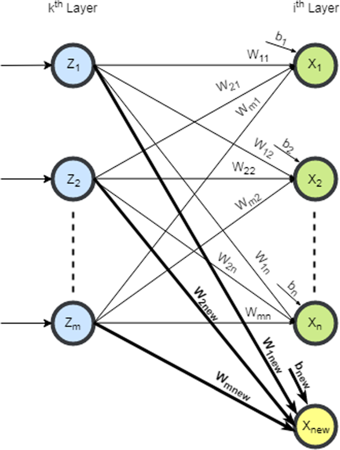

  

  Incoming weights to a newly added neuron

  Case II: The outgoing weight from a newly added neuron x_new in the ith layer to the neurons $u_{j} | j = 1 \ldots p,$ in the next layer, i.e. the jth layer as shown in Fig. 10, is calculated as:

  $$ w_{{{\text{new}}j}} = \mathop \sum \limits_{i = 1}^{n} {\raise0.7ex\hbox{${w_{ij} }$} \!\mathord{\left/ {\vphantom {{w_{ij} } n}}\right.\kern-0pt} \!\lower0.7ex\hbox{$n$}} $$

  (28)

  where n is number of neurons in the ith layer.

  Fig. 10

  

  Outgoing weights from a newly added neuron

  Case III: The outgoing weight from a new neuron to another new neuron in the next layer is chosen randomly in the range [− 5, 5] as shown in Fig. 11.

  Fig. 11

  

  Weights between two newly added neurons

  Biases of the newly added neurons in the hidden layers are initialized randomly between [−5, 5].

• b. Deletion of existing neurons: When one or more neurons are deleted from any layer, their corresponding incoming weights (in case of hidden neurons only), outgoing weights and biases are removed from the corresponding W vector.

Once all the W vectors are modified, NCSOA is applied again to obtain an optimal set of connection weights corresponding to each of the modified F&A vector. Let W^new be the new W vector corresponding to the modified F&A vector $F\& A^{\text{new}}$. Unlike the generation of initial population of W vectors in the first iteration of SM-GNCSOA, the initial population of W vectors for a particular $F\& A^{\text{new}}$ vector is generated greedily using $W^{\text{new}}$ vector, i.e. by choosing the weights and biases in the range $\left[ {W^{\text{new}} - 2, W^{\text{new}} + 2} \right]$ for each dimension of W vector. Instead of initializing the weights and biases randomly, they are chosen from the specified range to improve the convergence speed. This process is repeated until a stopping criterion is met. The algorithm of SM-GNCSOA is shown in Fig. 12.

Fig. 12

Algorithm of SM-GNCSOA

The computation complexity of SM-GNCSOA is obtained by calculating the computational complexity of NCSOA that is called by SM-GNCSOA for each F&A vector in every iteration and the computational complexity of SM-BGOA/GOA. The computational complexity of SM-GNCSOA is $O\left( {T^{2} N\left( {N_{SM } N_{SMP} + N_{TM} } \right)\left( {D_{W} + cof_{1} } \right)} \right)$. Here, the number of iterations of SM-GNCSOA and NCSOA is equal and is represented by T, N is population size, i.e. number of F&A vectors, $N_{SM}$ and N_TM are the number of cats in seeking mode and tracing mode, respectively, N_SMP is the number of copies of a cat that are made in seeking mode, D_W is the dimension of W vector, and cof₁ represents the cost of evaluation of fitness function of W vector.

5 Results and discussion

In Sect. 5.1, we discuss the data sets that are selected to evaluate the performance of the proposed algorithm. In Sect. 5.2, variants of SM-GNCSOA are presented. The implementation details and parameter settings are also presented in Sect. 5.2. Results are discussed in Sect. 5.3.

5.1 Data set

Ten classification problems are used to evaluate the performance of SM-GNCSOA and its variants. The data sets are selected from UCI data repository (Frank and Asuncion 2010). Out of ten data sets, five data sets are of binary classification, while the remaining five data sets are of multi-class classification problems. The data sets are: diabetes, diabetic retinopathy, Haberman’s survival, seismic bumps, Tic-Tac-Toe endgame, E. coli, Iris, wholesale customers, website phishing and statlog (Landsat satellite). The detail of each data set is presented in Table 2. To avoid overfitting, the total instances in the data set are divided into three parts. 75% instances are used for training, out of which 20% are set aside for validation. The remaining 25% instances in the data set are used for testing.

Table 2 Data sets

5.2 Experimental design and set-up

SM-GNCSOA is implemented in Python 3.6.4 using Anaconda framework. In order to appraise the effect of the proposed SM-BGOA, NCSOA and the use of penalty functions while generating an optimal MLP, we propose different variants of SM-GNCSOA and compare their training and testing classification accuracy with SM-GNCSOA. The details of SM-GNCSOA and its variant are presented in Table 3. SM-GNCSOA and B-GNCSOA compare the effect of SM-BGOA and BGOA, used for feature selection, on the performance of the classifier. The effect of NCSOA and CSOA, used for weight and bias optimization, is measured by comparing the classifier’s accuracies obtained using SM-GNCSOA and SM-GCSOA. The effect of using penalty function, namely architecture and feature penalty, on the classifier’s accuracy is evaluated using SM-GNCSOA and SM-GNCSOA-wp. Finally, to assess the effect of using NCSOA for training as compared to BP, the performance of SM-GNCSOA is compared with SM-GBP. To measure the accuracy of various classifiers, each algorithm is made to run on a data set for 30 times. A population size of 30 is taken, and the maximum number of iterations is taken as 300. The parameter settings of SM-BGOA, GOA and NCSOA used in SM-GNCSOA are shown in Table 4. Finally, for each data set, details of the best MLP (classifier) obtained during each of the 30 runs are noted for each algorithm and their classification accuracy is calculated using Eq. 29 by classifying the testing data. The classification accuracy of the classifier is calculated as:

Table 3 SM-GNCSOA and its variants

Table 4 Parameter settings

$$ {\text{Classification}} \;{\text{Accuracy}} = {\raise0.7ex\hbox{${\text{NCCTI}}$} \!\mathord{\left/ {\vphantom {{\text{NCCTI}} {\text{TNTI}}}}\right.\kern-0pt} \!\lower0.7ex\hbox{${\text{TNTI}}$}} $$

(29)

where NCCTI and TNTI are the number of correctly classified testing instances and total testing instances, respectively. Experiments are run on a computer with an Intel core i5 5200U processor running at 2.2 GHZ with 8 GB of RAM, running Ubuntu version 16.04.

5.3 Results and analysis

Out of the 30 best MLPs obtained during the 30 runs, the detail of the best MLP, i.e. the number of features selected (number of input neurons), architecture which includes the number of neurons in both the hidden layers and the transfer functions TF₁ and TF₂ of the first and second hidden layer obtained using SM-GNCSOA and its variants along with the number of output neurons on the ten data sets are presented in Table 5.

Table 5 Best MLPs architectures

The average classification accuracy, standard deviation and the best classification accuracy of the best MLPs obtained over 30 runs of SM-GNCSOA and its variants on ten data sets are given in Table 6. It can be seen from Table 5 the MLP generated using SM-GNCSOA-wp has complex architecture and a greater number of features got selected compared to SM-GNCSOA and its other variants as there is no penalty for complex architecture and number of features selected in SM-GNCSOA-wp. However, complex architecture and a greater number of features do not necessarily result in the improvement of the performance of MLP as can be seen from Table 6. In case of data sets like diabetic retinopathy, seismic bumps and statlog (Landsat satellite) where the number of features is more, SM-GNCSOA-wp performs better than SM-GNCSOA and its other variants which uses feature and architecture penalty. This is due to the fact that unlike SM-GNCSOA-wp, SM-GNCSOA and its other variants prevent complex architecture and selection of large number of features which may lead to reduction in performance of the MLP. In case of Iris data set, the best classification accuracy obtained using SM-GNCSOA, B-GNCSOA and SM-GNCSOA-wp is same (100%); however, the architecture of MLP obtained using SM-GNCSOA-wp is much more complex than the MLP obtained using SM-GNCSOA and B-GNCSOA in terms of numbers of neurons in hidden layers This shows that it is not necessary that a complex architecture will always perform better than simple architecture as complex architecture sometimes leads to overfitting.

Table 6 Classification accuracy of SM-GNCSOA and its variants

While comparing the results of MLP obtained using SM-GNCSOA and SM-GCSOA, it can be observed from Table 6 that SM-GNCSOA outperforms SM-GCSOA. Even in case of a small data set, i.e. Iris data set, which has only four features, the performance of SM-GNCSOA, B-GNCSOA and SM-GNCSOA-wp is comparable, whereas SM-GCSOA performance is sub-optimal. The sub-optimal performance of SM-GCSOA is due to the tendency of CSOA in getting trapped in local optima during weight optimization which results in sub-optimal solutions, while the proposed algorithm NCSOA avoids local optima by introducing diversity in the population using an adaptive parameter N leading to better exploration. The parameter N is designed in such a way that it favours exploitation in later iterations and helps in maintaining a balance between exploration and exploitation leading to better performance of NCSOA than CSOA.

The performance of MLP obtained using SM-GNCSOA is better than the MLP obtained using B-GNCSOA as can be seen in Table 6. In GOA, the social interaction, i.e. attraction (exploitation) and repulsion (exploration), of grasshopper depends on the social force which is a function of distance between the grasshoppers. Unlike BGOA in B-GNCSOA that uses Euclidean distance to calculate the distance between grasshoppers, SM-BGOA in SM-GNCSOA uses SMD to calculate the distances between the feature vector part of F&A vectors that helps in performing exploration and exploitation properly thereby resulting in improved performance of SM-GNCSOA as compared to B-GNCSOA. It can also be seen in Table 6 that NCSOA used for optimization of weight vector gives better results as compared to BP as BP also has a tendency to get stuck in local optima hence leading to sub-optimal solution.

To ensure that the comparison between the metaheuristics is fair, Welch’s t test is performed at α = 0.05 on the classification accuracy of best MLPs obtained by SM-GNCSOA and its variants over 30 runs for each data set given in Table 2. The results of Welch’s t test are shown in Table 7. The statistical results (p values < 0.05) confirm that the performance of SM-GNCSOA on diabetes, Haberman’s survival, Tic-Tac-Toe endgame, E. coli, wholesale customer’s and website phishing is significantly better than its variants. In case of data sets like diabetic retinopathy, seismic bumps and statlog (Landsat satellite) which have large number of features, the results of Welch’s t test confirm that SM-GNCSOA-wp performs better than SM-GNCSOA and other variants. On the Iris data set, although the best classification accuracy achieved by SM-GNCSOA, B-GNCSOA and SM-GNCSOA-wp is equal, the average classification accuracy of B-GNCSOA and SM-GNCSOA-wp is better than SM-GNCSOA. However, the statistical results with p value equal to 0.2388 and 0.3014 for B-GNCSOA and SM-GNCSOA-wp in Table 7 indicate that the difference is insignificant, but the performance of SM-GNCSOA is significantly better than that of SM-GCSOA and SM-GBP in case of Iris data set as can be seen in Table 7.

Table 7 Result of Welch’s t test at α = 0.05 on classification accuracy of SM-GNCSOA versus its variants

As each algorithm runs, the total loss calculated using Eq. 26, training error and validation error calculated using Eq. 22 for binary classification and Eq. 23 for multi-class classification on training and validation data, respectively, of best MLP obtained using SM-GNCSOA and its variants on all the ten data sets are noted at an interval of 30 iterations and are plotted to visualize the convergence rate as shown in Figs. 13, 14 and 15, respectively. SM-GNCSOA has a faster convergence rate as compared to B-GNCSOA. It is evident from Fig. 14 that CSOA in SM-GCSOA and BP in SM-GBP used for optimization of W vector often gets stuck into local optima leading to premature convergence. It can be seen from Fig. 15, sometimes the validation error increases during the optimization process due to overfitting which incurs more penalty to the MLP thereby reducing its fitness. Graphs showing the variation in architecture penalty and feature penalty are plotted as shown in Figs. 16 and 17, respectively. It can be inferred from these graphs that the number of features and the number of hidden neurons increase and decrease during the optimization process.

Fig. 13

Convergence graphs of total loss of ten data sets

Fig. 14

Convergence graphs of training error of ten data sets

Fig. 15

Convergence graphs of validation loss of ten data sets

Fig. 16

Graphs of architecture penalty of ten data sets

Fig. 17

Graphs of feature penalty of ten data sets

Finally, confusion matrix of the performance of best MLPs on testing data for each of the ten data sets is plotted as shown in Fig. 18. Confusion matrix is plotted to define the performance of a classifier on a set of testing instances for which the true class labels are known. It depicts the number of correctly classified as well as incorrectly classified instances of the data set for binary as well as multi-class classification problems.

Fig. 18

Confusion matrix of ten data sets on the best MLPs

The main limitation of SM-GNCSOA is its high computational complexity. SM-GNCSOA is a hybrid algorithm in which SM-BGOA is used for feature optimization, GOA is used for architecture and transfer functions optimization, and NCSOA is used for weight optimization corresponding to each F&A vector. SM-GNCSOA calls NCSOA for each F&A vector in every iteration, which increases its computational complexity.

6 Conclusion and future work

In this paper, SM-BGOA and NCSOA, a variant of BGOA and CSOA, respectively, are proposed. Then, a hybrid algorithm SM-GNCSOA is proposed that uses SM-BGOA, GOA and NCSOA with two penalty functions to optimize feature set, architecture and weights of an MLP simultaneously. To prevent complex architecture, an architecture penalty function is introduced that penalizes complex architecture and reduces the fitness of the MLP. Similarly, to avoid underfitting and overfitting, a feature penalty function is used that imposes a penalty on the fitness of the MLP based on the number of features selected. A set of ten data sets are selected from UCI repository to evaluate the performance of SM-GNCSOA. The classification accuracy of the MLP obtained using SM-GNCSOA is compared with the MLPs obtained using variants of SM-GNCSOA.

The results show that SM-GNCSOA outperforms B-GNCSOA on almost all the data sets in terms of classification accuracy except Iris where the performance is comparable. SM-GNCSOA managed to show superior results due to its capability in performing exploration and exploitation effectively by calculating the strength of social forces between the grasshoppers more accurately. While comparing the performance of SM-GNCSOA and SM-GCSOA, the results show that SM-GNCSOA outperforms SM-GCSOA even in case of a small data set like Iris as NCSOA used for weight optimization in SM-GNCSOA explores the search space more efficiently and has high local optima avoidance as compared to CSOA that is used for weight optimization in SM-GCSOA. In case of data sets with large number of features like diabetic retinopathy, seismic bumps and statlog, the MLPs obtained by SM-GNCSOA-wp perform better as compared to SM-GNCSOA. It is due to the fact that sometimes all or most of the features contribute to the classification process and a complex architecture is also required. As SM-GNCSOA-wp does not incur penalties on selection of large number of features and a complex architecture, hence, it performs better in cases of data sets with large number of attributes. The result of statistical test further proves the effectiveness of our proposed approach.

In future, we plan to implement other metaheuristic algorithms to generate MLPs and compare the performance of SM-GNCSOA with them. We also plan to use metaheuristic algorithms to optimize other types of ANNs.

References

Aljarah I, Faris H, Mirjalili S (2018) Optimizing connection weights in neural networks using the whale optimization algorithm. Soft Comput 22:1–15
Arora S, Anand P (2018) Chaotic grasshopper optimization algorithm for global optimization. Neural Comput Appl. https://doi.org/10.1007/s00521-018-3343-2
Bansal P, Gupta S, Kumar S, Sharma S, Sharma S (2019) MLP-LOA: a metaheuristic approach to design an optimal multilayer perceptron. Soft Comput. https://doi.org/10.1007/s00500-019-03773-2
Cai J, Luo J, Wang S, Yang S (2018) Feature selection in machine learning: a new perspective. Neurocomputing 300:70–79
Carvalho M, Ludermir T (2007) Particle swarm optimization of neural network architectures and weights. In 7th International conference on hybrid intelligent systems, pp 336–339
Chen L-H, Zhang XY (2009) Application of artificial neural network to classify water quality of the yellow river. In: Fuzzy information and engineering. Advances in soft computing, vol 54, pp 15–23
Choi S, Cha S, Tappert CC (2010) A survey of binary similarity and distance measures. J Syst Cybern Inform 8(1):43–48
Chu SC, Tsai PW, Pan JS (2006) Cat swarm optimization. In: Pacific Rim international conference on artificial intelligence. Springer, Berlin, pp 854–858
Ewees AA, Elaziz MA, Houssein EH (2018) Improved grasshopper optimization algorithm using opposition-based learning. Expert Syst Appl 112:156–172
Faris H, Aljarah I, Mirjalili S (2016) Training feedforward neural networks using multi-verse optimizer for binary classification problems. Appl Intell 45(2):322–332
Faris H, Aljarah I, Mirjalili S (2017) Improved monarch butterfly optimization for unconstrained global search and neural network training. Appl Intell 48:445–468
Faris H, Mafarja MM, Heidari AA, Aljarah I, Ala’M AZ, Mirjalili S, Fujita H (2018) An efficient binary salp swarm algorithm with crossover scheme for feature selection problem. Knowl-Based Syst 154:43–67
Frank A, Asuncion A (2010) UCI machine learning repository [http://archive.ics.uci.edu/ml]. University of California, School of Information and Computer Science, Irvine, CA
Gandomi AH, Alavi AH (2012) Krill herd: a new bio-inspired optimization algorithm. Commun Nonlinear Sci Numer Simul 17(12):4831–4845
Garro BA, Vázquez RA (2015) Designing artificial neural networks using particle swarm optimization algorithms. Comput Intell Neurosci. https://doi.org/10.1155/2015/369298
Garro BA, Sossa H, Vazquez RA (2011) Artificial neural network synthesis by means of artificial bee colony (abc) algorithm. In: Proceedings of the IEEE congress on evolutionary computation (CEC’11), pp 331–338
Ghaemi M, Feizi-Derakhshi M-R (2016) Feature selection using forest optimization algorithm. Pattern Recogn 60:121–129. https://doi.org/10.1016/j.patcog.2016.05.012
Guo L, Meng Z, Sun Y, Wang L (2018) A modified cat swarm optimization based maximum power point tracking method for photovoltaic system under partially shaded condition. Energy 144:501–514
Hacibeyoglu M, Ibrahim MH (2018) A novel multimean particle swarm optimization algorithm for nonlinear continuous optimization: application to feed-forward neural network training. Sci Program. https://doi.org/10.1155/2018/1435810
Han J, Kamber M (2006) Data mining: concepts and techniques. Elsevier Inc (chapter 7)
Heaton J (2008) Introduction to neural networks with java
Heidari AA, Faris H, Aljarah I, Mirjalili S (2018) An efficient hybrid multilayer perceptron neural network with grasshopper optimization. Soft Comput. https://doi.org/10.1007/s00500-018-3424-2
Hong CM, Chen CM, Fan HK (1999) A new gradient-based search method: grey-gradient search method. In: Imam I, Kodratoff Y, El-Dessouki A, Ali M (eds) Multiple approaches to intelligent systems. IEA/AIE 1999. Lecture notes in computer science, vol 1611. Springer, Berlin
Islam MM, Sattar MA, Amin MF, Yao X, Murase K (2009a) A new constructive algorithm for architectural and functional adaptation of artificial neural networks. IEEE Trans Syst Man Cybern Part B Cybern 39(6):1590–1605
Islam MM, Sattar MA, Amin MF, Yao X, Murase K (2009b) A new adaptive merging and growing algorithm for designing artificial neural networks. IEEE Trans Syst Man Cybern Part B Cybern 39(3):705–722
Jaddi NS, Abdullah S, Hamdan AR (2015a) Multi-population cooperative bat algorithm-based optimization of artificial neural network model. Inf Sci 294:628–644
Jaddi NS, Abdullah S, Hamdan AR (2015b) Optimization of neural network model using modified bat-inspired algorithm. Appl Soft Comput 37:71–86
Karaboga D (2005) An idea based on honey bee swarm for numerical optimization. Technical report-TR-06. Engineering Faculty, Computer Engineering Department, Erciyes University
Karaboga D, Akay B, Ozturk C (2007) Artificial bee colony (ABC) optimization algorithm for training feed-forward neural networks. In: Modeling decisions for artificial intelligence. Springer, Berlin, pp 318–329
Karlik B, Olgac AV (2010) Performance analysis of various activation functions in generalized MLP architectures of neural networks. Int J Artif Intell Expert Syst 1:111–122
Katrutsa A, Strijov V (2017) Comprehensive study of feature selection methods to solve multicollinearity problem according to evaluation criteria. Expert Syst Appl 76:1–11
Kohavi R, John G (1997) Wrappers for feature subset selection. Artif Intell 97(12):273–324
Kumar Y, Singh PK (2018) Improved cat swarm optimization algorithm for solving global optimization problems and its application to clustering. Appl Intell 48(9):2681–2697
Lauret P, Fock E, Mara TA (2006) A node pruning algorithm based on a Fourier amplitude sensitivity test method. IEEE Trans Neural Netw 17(2):273–293
Liu H, Motoda H (1998) Feature selection for knowledge discovery and data mining. Kluwer, Boston
Luo J, Chen H, Zhang Q, Xu Y, Huang H, Zhao XA (2018) An improved grasshopper optimization algorithm with application to financial stress prediction. Appl Math Model 64:654–668
Ma L, Khorasani K (2005) Constructive feedforward neural networks using Hermite polynomial activation functions. IEEE Trans Neural Netw 16(4):821–833
Mafarja MM, Mirjalili S (2017) Hybrid whale optimization algorithm with simulated annealing for feature selection. Neurocomputing 260:302–312
Mafarja M, Mirjalili S (2018) Whale optimization approaches for wrapper feature selection. Appl Soft Comput 62:441–453
Mafarja M, Aljarah I, Faris H, Hammouri AI, Ala’M AZ, Mirjalili S (2018) Binary grasshopper optimisation algorithm approaches for feature selection problems. Expert Syst Appl 117:267–286
Mirjalili S (2015a) How effective is the grey wolf optimizer in training multi-layer perceptrons. Appl Intell 43(1):150–161. https://doi.org/10.1007/s10489-014-0645-7
Mirjalili S (2015b) Moth-flame optimization algorithm: a novel nature-inspired heuristic paradigm. Knowl-Based Syst. https://doi.org/10.1016/j.knosys.2015.07.006
Mirjalili S, Mirjalili SM, Yang XS (2014a) Binary bat algorithm. Neural Comput Appl 25:663. https://doi.org/10.1007/s00521-013-1525-5
Mirjalili S, Mirjalili SM, Lewis A (2014b) Grey wolf optimizer. Adv Eng Softw 69:46–61
Mirjalili SZ, Mirjalili S, Saremi S, Faris H, Aljarah I (2017) Grasshopper optimization algorithm for multi-objective optimization problems. Appl Intell 1–16
Mirzaei A, Mohsenzadeh Y, Sheikhzadeh H (2017) Variational relevant sample-feature machine: a fully Bayesian approach for embedded feature selection. Neurocomputing 241:181–190
Orouskhani M, Orouskhani Y, Mansouri M, Teshnehlab M (2013) A novel cat swarm optimization algorithm for unconstrained optimization problems. Inf Technol Comput Sci 5(11):32–41
Passino KM (2002) Biomimicry of bacterial foraging for distributed optimization and control. IEEE Control Syst Mag 22(3):52–67
Rezaeianzadeh M, Tabari H, Arabi YA, Isik S, Kalin L (2014) Flood flow forecasting using ANN, ANFIS and regression models. Neural Comput Appl 25(1):25–37
Saha SK, Ghoshal SP, Kar R, Mandal D (2013) Cat swarm optimization algorithm for optimal linear phase fir filter design. ISA Trans 52:781–794
Saremi S, Mirjalili S, Lewis A (2017) Grasshopper optimisation algorithm: theory and application. Adv Eng Softw 105:30–47
Schmidhuber J (2015) Deep learning in neural networks: an overview. Neural Netw 61:85–117
Tharwat A, Houssein EH, Ahmed MM, Hassanien AE, Gabel T (2017) MOGOA algorithm for constrained and unconstrained multi-objective optimization problems. Appl Intell 48:1–16
Tsai JT, Chou JH, Liu TK (2006) Tuning the structure and parameters of a neural network by using hybrid Taguchi-genetic algorithm. IEEE Trans Neural Netw 17(1):69–80
Vázquez JC, López M, Melin P (2010) Real time face identification using a neural network approach. In: Melin P, Kacprzyk J, Pedrycz W (eds) Soft computing for recognition based on biometrics. Studies in computational intelligence, vol 312. Springer, Berlin
Wdaa ASI (2008) Differential evolution for neural networks learning enhancement. Ph.D. thesis, Universiti Teknologi, Malaysia
Wolpert DH, Macready WG (1997) No free lunch theorems for optimization. IEEE Trans Evol Comput 1(1):67–82
Wu J, Wang H, Li N, Yao P, Huang Y, Su Z, Yu Y (2017) Distributed trajectory optimization for multiple solar-powered UAVs target tracking in urban environment by Adaptive Grasshopper Optimisation Algorithm. Aerosp Sci Technol. https://doi.org/10.1016/j.ast.2017.08.037
Xue B, Zhang M, Browne WN (2013) Particle swarm optimisation for feature selection in classification: novel initialisation and updating mechanisms. Appl Soft Comput 18:261–276
Yang XS. (2009) Firefly algorithms for multimodal optimization. In: Watanabe O, Zeugmann T (eds) Stochastic algorithms: foundations and applications. SAGA 2009. Lecture notes in computer science, vol 5792. Springer, Berlin
Zanchettin C, Ludermir TB, Almeida LM (2011) Hybrid training method for MLP: optimization of architecture and training. IEEE Trans Syst Man Cybern Part B Cybern 41(4):1097–1109
Zarshenas A, Suzuki K (2016) Binary coordinate ascent: an efficient optimization technique for feature subset selection for machine learning. Knowl-Based Syst 110:191–201
Zhang L, Liu L, Yang X-S, Dai Y (2016) A novel hybrid firefly algorithm for global optimization. PLoS ONE 11(9):1–17
Author information
Authors and Affiliations
Corresponding author
Ethics declarations
Conflict of interest
All authors declare that they have no conflict of interest.
Ethical approval
This article does not contain any studies with human participants or animals performed by any of the authors.
Additional information
Communicated by V. Loia.
Publisher's Note
Springer Nature remains neutral with regard to jurisdictional claims in published maps and institutional affiliations.
Rights and permissions
About this article
Cite this article
Bansal, P., Kumar, S., Pasrija, S. et al. A hybrid grasshopper and new cat swarm optimization algorithm for feature selection and optimization of multi-layer perceptron. Soft Comput 24, 15463–15489 (2020). https://doi.org/10.1007/s00500-020-04877-w
Published:
Issue Date:
DOI: https://doi.org/10.1007/s00500-020-04877-w