
Abstract
The consistent and efficient method for the identification of biometrics is the iris recognition in view of the fact that it has richness in texture information. A good number of features performed in the past are built on handcrafted features. The proposed method is based on the feed-forward architecture and uses k-means clustering algorithm for the iris patterns classification. In this paper, segmentation of iris is performed using the circular Hough transform that realizes the iris boundaries in the eye and isolates the region of iris with no eyelashes and other constrictions. Moreover, Daugman’s rubber sheet model is used to transform the resultant iris portion into polar coordinates in the process of normalization. A unique iris code is generated by log-Gabor filter to extract the features. The classification is achieved using neural network structures, the feed-forward neural network and the radial basis function neural network. The experiments have been conducted using the Chinese Academy of Sciences Institute of Automation (CASIA) iris database. The proposed system decreases computation time, size of the database and increases the recognition accuracy as compared to the existing algorithms.
1 Introduction
These days, safety is the substantial aspect in the fields of information technology, commerce, business and military, etc. (Galbally et al. 2014; Gupta and Gupta 2014; Eastwood et al. 2016; Hurtado et al. 2010; Liu et al. 2016; Cho et al. 2005; Mock et al. 2012; Xiao 2007; Poursaberi et al. 2013; Wildes et al. 1994; Basit et al. 2005; Roh et al. 2016; Tripathi 2017; Jain et al. 2004). Various measures of identification such as ID card, password, signature and PIN are broadly used which have definite limitations; these methods can be lost or stolen or faked, but biometric parameters are more secure and reliable in personal identification. Biometrics is proved to be the safe and the best means for the important documents. Several corporations have adopted biometrics to safeguard their personal assets. The applications of biometric recognition can be observed in healthcare and welfare, public safety, finance and banking, immigration and border control and attendance management.
Iris recognition is an efficient and reliable approach for the biometric identification. Iris is a thin structure in the eye, and it has abundant properties which makes it eventual biometrics recognition. Figure 1 displays the iris region lying in the middle of the sclera and the pupil. The human iris is unalterable and steady from birth till death. The characteristics which make iris as good biometrics for the identification of an individual are: high exclusivity and steadiness, the features of right to left eye is not identical. Iris when compared with accompanying biometrics for instance face, speech recognition and fingerprint is considered as the faithful manner of biometrics technology.

Human iris
In this paper, we propose a simple and efficient algorithm based on classification approaches, the feed-forward neural network and the radial basis function neural network for the best accurate results. In particular, (1) we first implement the pre-processing in which it develops the proficiency for the machine to identify the objects and feature that include histogram equalization, intensity, static gamma correction and noise removal. (2) The Hough transform in segmentation accurately segregates the region of iris from the image of an eye. A system is needed which separates and eliminates the artefacts. An integro-differential operator searches the iris and the pupil boundaries. (3) Normalization locates the outer and inner borders to compensate the capturing distance and varying pupil size. As per the Daugman’s rubber sheet model, each pixel is mapped into a pair of polar coordinates. (4) In feature extraction, the features of the iris are extracted and generate the iris code. (5) In our proposed classification approach, we have classified the features with feed-forward neural network and radial basis function neural network that compares the iris that is already stored and checks the current iris image whether it belongs to the same class or not. RBFNN is found to have better recognition accuracy than any other single method. The flowchart of Iris recognition is shown in Fig. 2.

Flowchart of the iris recognition
The motivation of this paper is that all the old techniques are complex and have slow performance and takes more computational time, so the technique used in this paper has improved the complexity, has less computational time and is more appropriate for the applications.
The paper is structured in the following manner. In Sect. 2, the previous related work of the iris recognition system is mentioned. In Sect. 3, we momentarily overview a number of representative works on image acquisition, segmentation, feature encoding and classification. In Section 4, the details of the artificial neural network, the feed-forward neural network and the radial basis function neural network are explained. In Sect. 5, we account the experimental results of the proposed method and finally in Sect. 6, we conclude the paper.
2 Related work
Daugman (1992, 1993, 1994, 2001, 2004, 2007, 2016) proposed capturing images of the eye at very close range using a video camera and point light source. The system operator would then manually select the center of the pupil. The close range reduces interference from ambient light, and the manual selection speeds up and simplifies the segmentation process. Once the iris image was captured, a series of integro-differential operators, which show where the largest gradients are in the image, would be used to segment the iris. The iris would be removed from the image and normalized to a rectangular form. This operation would remove artefacts, such as eyelashes and other ‘noise,’ and simplify the comparison process. This unwrapped iris image would then be encoded using two-dimensional Gabor filters, so converting the iris from a complicated multi-level bitmap image into a much simpler binary code. This encoded iris could then be compared to other encoded irises by calculating the fraction of bits that disagree, called the Hamming distance. Daugman published two papers (Daugman 2004, 2016) about iris recognition methodology. US patent 5,291,560 was granted allowing Flom, Safir and Daugman to set up a company and license the technology for commercial implementation. Figure 3 shows the iris recognition system.

Iris recognition system
Daouk et al. (2002) used Hough transform and a canny edge detection scheme to identify digital image of an eye and then applied the Haar wavelet to define patterns in the iris of a person to determine patterns in an individual’s iris from the feature vector through associating the quantized vectors using the Hamming distance operator.
Abiyev and Altunkaya (2008) projected a new iris recognition system which is based on neural network (NN). The iris patterns are classified with the NN. The benefit of this method is that iris segmentation is achieved in less time.
Ma et al. (2004) described an efficient algorithm for iris recognition by characterizing key local variations and denoted the appearing and vanishing of an important image structure, utilized to represent the characteristics of the iris.
Zhu et al. (2000) presented a new system which is composed of iris acquisition, image pre-processing, feature extraction and classifier. The feature extraction is based on texture analysis using multi-channel Gabor filtering and wavelet transform.
According to Sundaram and Dhara (2011), in the first step, the localization of iris is done by the circular Hough transform. In the succeeding step, Daugman’s rubber sheet model normalizes an image into a fixed Dimension and then 2-D Haar wavelet is used to decompose the normalized image to extract the textual features. The NN is used for the matching.
3 Proposed iris recognition
There are five steps in the proposed iris recognition system: the image pre-processing, the image segmentation, the iris normalization, the feature extraction and the classification. Figure 4 shows the steps involved in the proposed iris recognition system.

Proposed iris recognition system
3.1 Iris image from database
The iris capture step is normally carried out using a camera. Sometimes, this camera is a still-capture device, and sometimes it is a video camera. In general, this step is handled by using pre-captured images. CASIA version 1.0 and version 4.0 database has been used for the recognition system. Iris database version 1.0 consists of 756 iris images from 108 eyes captured with their close-up camera, and database version 4.0 consists of 2639 iris samples from 39 classes of 249 volunteers.
3.2 Image pre-processing
Having captured or loaded the eye image, the next stage is pre-processing. Images are preprocessed in order to improve the ability of the machine to detect features and objects. Pre-processing can be as simple as intensity adjustments such as intensity stretching, histogram equalization, noise removal, edge detection and static gamma correction. Out of these techniques, we are using gamma correction for image pre-processing.
Gamma correction adjusts the intensity of all the pixels within an image, but the adjustment is nonlinear. Equation 1 is the calculation for gamma correction.
where I (x, y) is the original image, γ is the correction value, and G (x, y) is the gamma-corrected image. If γ is greater than one, then the darker intensities will be compressed so that their values are closer together, but the higher intensities will be stretched further apart. This will give an image where the brighter intensities are easier to discern but the darker ones become more difficult to separate. If γ is less than one, then the brighter intensity pixels will have their values compressed together, while the darker intensity pixels will have their values stretched further apart. This will give an image that is brighter overall, where the brighter intensities may become much clear and brighter. Within the process of iris recognition, image pre-processing is different from the other stages. Even though it is placed between image capture and segmentation, it may be carried out several times during and after the segmentation process.
3.3 Iris segmentation
Iris segmentation (Daugman 2004, 2007; Daouk et al. 2002; Abiyev and Altunkaya 2008; Masek 2003; Abhyankar et al. 2005; Vatsa et al. 2007; Nguyen Thanh et al. 2010; Punyani and Gupta 2015; Chawla and Oberoi 2011; Schlett et al. 2018) segregates the region of iris from the image of an eye. The eyelids and eyelashes obstruct the iris region portion, and specular reflections so occurred can fraudulent the iris patterns. A method is required that excludes and isolates the circular regions of iris and the artefacts.
3.3.1 Integro-differential operator
John Daugman developed the fundamental iris algorithm for recognition system. Daugman et al. using integro-differential operator is a thoroughly examined and best-known iris segmentation method. It is a circular edge detector, used to identify the outer and inner boundaries of the iris. It can also define the elliptical boundaries of the eyelids. An integro-differential operator can be expressed as in Eq. 2:
where r is the radius to search, \( G_{\sigma } (r) \) is a Gaussian smoothing function with the factor \( \sigma \), and I(x, y) is the image of an eye in the contour of the circle which is given as \( (r,x_{0} ,y_{0} ) \). The input image for a circle is scanned by this operator which is having a maximum gradient change with center coordinates \( (x_{0} ,y_{0} ) \) and a circular arc ds of radius r. The process of segmentation commences with the outer boundaries located between the white sclera and the iris. High contrast is obtained when \( \sigma \) is fixed, for investigation and to detect the outer boundary. As the presence of the eyelashes and eyelids meaningfully raises the gradient so computed and this do not restrict the affected area. The output of segmentation using integro-differential operator is shown in Fig. 5.


Segmentation output using an integro-differential operator
3.3.2 Hough transform
The linear Hough transform (López et al. 2013; Chawla and Oberoi 2011; Sharma and Monga 2014; Shylaja et al. 2011) recognizes the geometrical objects for instance circles and lines. The circular Hough transform realizes the center coordinates and radius of the pupil and the iris. An edge map that produces the threshold result is evaluated by the first derivative of the intensity value in the image. Equation 3 defines the center coordinates \( x_{\text{c}} \) and \( y_{\text{c}} \) and radius of the image.
The center points are defined by maximum points in the Hough space, and the radius is defined by the edge points. The inner iris/sclera boundaries are equally weighted to generate an edge map using the vertical and the horizontal gradients in the canny edge detection. For an accurate and the efficient recognition, the Hough transform is performed for the iris/sclera first and then for the iris/pupil boundary. The segmentation using the Hough transform is shown in Fig. 6.


Output of Hough transform using canny edge detector
3.4 Iris normalization
The normalization (Chawla and Oberoi 2011; Sharma and Monga 2014; Boles and Boashash 1998) locates the outer and inner borders to reimburse the varying size and capturing distance. The size of iris of the same eye might change because of the distance from the camera, illumination, variations, etc. The non-concentric characteristics of iris and the pupil may affect the result of matching. According to Daugman’s rubber sheet model, each pixel is mapped into a pair of polar coordinates \( (r,\theta ) \), where r has the interval [0,1] and \( \theta \) on the interval \( [0,2\pi ] \) as shown in Fig. 7.

Daugman’s rubber sheet model
The unwrapping formula is as follows:
where
where \( x(r,\theta ) \) and \( y(r,\theta ) \) are the combinations between the coordinates of the pupillary boundary \( (x_{p} (\theta ),y_{p} (\theta )) \) and the coordinates of the iris boundary \( (x_{i} (\theta ),y_{i} (\theta )) \), in the direction \( \theta \) while \( r_{p} \) and \( r_{i} \) are the radius of the pupil and the iris, respectively, and \( (x_{{p_{0} }} ,y_{{p_{0} }} ) \), \( (x_{{i_{0} }} ,y_{{i_{0} }} ) \) are the centers of pupil and iris, respectively, in Eqs. (5–7).
As the pupil is non-concentric as compared to the iris, we need a remapping formula to rescale points that depends on the angle round the circle given by Eqs. (8–9).
where \( r' \) is the distance between the edge of the pupil and edge of the iris at an angle \( \theta \) around the region, the displacement of the center of the pupil relative to the center of the iris is given by \( o_{x} ,o_{y} \), and \( r_{I} \) is the radius of the iris as shown in Fig. 8. The output of the normalization of the iris image using the remapping formula is shown in Fig. 9.


Daugman’s rubber sheet model providing pupil displacement correction showing exaggerated pupil displacement for illustration

Normalization output
3.5 Feature extraction
Owing to the circumstances of light sources and consequence of imaging conditions, the normalized iris image does not have an appropriate quality. The noise marks while taking the image some light illusion and noise results are removed during the enhancement process. It is necessary to enhance the extracted patterns of the iris image. The encoding (Hu et al. 2017; Kushwaha and Welekar 2016; Kyaw 2009; Gupta and Gupta 2016) normalizes and convolves the iris image after normalization with 1D Gabor log-wavelet filter. It is achieved by extracting the frequency information of an image by Gabor filter and assessing the definite bands of the power–frequency, and in spatial domain it gives the result of the location. The sequence of 1D signal aliens the 2D normalized pattern; these signals are convolved with parameters that allow coverage of the spectrum which is constant as shown in Fig. 10.

a The normalization and b feature extraction output of CASIA dataset
The first step in the construction of the filter is to compute the frequency values which ranges from 0 to 0.5 with the radial components and then estimate the cutoff frequency f0 of the filter, and the normalized radius at cutoff frequency domain can be built in the spatial domain at cutoff frequency and can be mathematically made by the inverse Fourier transform in the spatial domain in Eq. 10.
Hence, \( \sigma \) signifies the bandwidth of the filter in the radial direction and f0 denotes the cutoff frequency of the filter.

4 Artificial neural network (ANN)
ANN (Shylaja et al. 2011; Haddouch et al. 2016) has n inputs, denoted as \( x_{1} ,x_{2} , \ldots ,x_{n} \). Each connecting line to the neuron is denoted by \( w_{1} ,w_{2} , \ldots ,w_{n} \), respectively(denoted by Fig. 11).

Neuron model used in artificial neural network
The formula in Eq. 11 governs whether the neuron is to be fired or not.
The output of the neuron is a function of its action as shown in Eq. 12:
where f(a) is a threshold function of the neuron.
In this paper, classification is solved by two types of neural networks.
4.1 Feed-forward neural network (FNN)
Feed-forward neural network (Shylaja et al. 2011; Njikam and Zhao 2016; Wang et al. 2003) has been used for iris feature classification. FNN is one of the popular structures among artificial neural networks. The information in this network moves only in one direction, i.e. forward from the input nodes through the hidden nodes and to the output nodes as shown in Fig. 12.

Feed-forward neural network architecture
4.2 Radial basis function neural network (RBFNN)
The radial basis function neural network (Yu et al. 2016; Chen 2017; Wang et al. 2003) is feed-forward architecture with an input layer, an output layer and a hidden layer as in Fig. 13. Each of the layers implements a radial basis function. The input layer of this network has \( n_{i} \)-dimensional input vectors and is fully connected to the \( n_{h} \) hidden layer units, which in turn connected to the \( n_{o} \) output layer.

Radial basis function neural network
The Gaussian function is chosen for the activation function of the hidden layer and is characterized by its mean vectors (centers) \( \mu_{i} \) and covariance matrices \( C_{i} ,i = 1,2, \ldots ,n_{h} \). It is assumed that the covariance matrices are of the form \( C_{i} = \sigma^{2}_{i} I,i = 1,2, \ldots ,n_{h} \). Then, the activation function of the \( i^{th} \) hidden unit for an input vector \( x_{j} \) is given by Eq. 13.
A suitable clustering algorithm is used to calculate \( \mu_{i} \) and \( \sigma_{i}^{2} \). The k-means clustering here is working to regulate the centers.

The smoothness of the mapping is influenced by the number of activation functions and their spread. The assumption \( \sigma_{i}^{2} = \sigma^{2} \) is made, and \( \sigma^{2} \) is given in mapping. σ 2 i = σ2 is made, and this ensures that activation function is not too peaked or too flat.
In Eq. 14, d is the maximum distance between the centers so chosen and \( \eta \) is an empirical scale factor which is served to control the smoothness of the mapping function. Equation 15 therefore can be written as:
The output layer units \( n_{c} \) are fully connected to the hidden layer units through the weights \( w_{ik} \). The output units are linear, and the response of the kth output unit for an input \( x_{i} \) is given by Eq. 16.
Here, \( g_{0} (x_{i} ) = 1 \). It is given that \( n_{t} \) iris features vectors from \( n_{c} \) subjects, training the radial basis function neural network which involves estimating \( \mu_{i} ,i = 1,2, \ldots ,n_{h} ,\eta ,d^{2} \) and \( w_{ik} ,i = 1,2, \ldots ,n_{h} ,k = 1,2, \ldots ,n_{c} \).
The weights \( w_{lk} \) between the hidden and the output units are determined. Given that the Gaussian function centers and width are calculated form \( n_{t} \) training vectors, can be written in matrix form as in Eq. 17.
Here, G is a \( n_{t} \times (n_{h} + 1) \) matrix with element \( G_{ij} = y_{j} (x_{i} ) \), Y is a \( n_{t} \times n_{c} \) matrix with elements \( Y_{ij} = y_{j} (x_{i} ) \), and W is a \( (n_{h} + 1) \times n_{c} \) matrix of unknown weights. W is obtained from the standard least squares solution as given by Eq. 18.
5 Experimental results
Our proposed work is carried out using MATLAB (R2014a) of Mathworks. Several datasets are available from these sources: Chinese Academy of Sciences Institute of Automation (CASIA), Multimedia University (MMU), Unconstrained Biometrics: Iris (UBIRIS), West Virginia University (WVU), Indian Institute of Technology (IIT) Delhi, University of Palackeho and Olomouc (UPOL), Iris Challenge Evaluation (ICE). To test the performance of the proposed algorithm, CASIA images from the database version 1.0 and version 4.0 have been used. A database version 1.0 comprises 756 images of iris from 108 eyes collected over two sessions with their close-up camera. The format of the captured image is BMP with the resolution of 320*280. Eight 850-nm circularly arranged nearest infrared illuminations are organized round the sensor to ensure the uniformly and illuminated iris pattern which protects the iris pattern recognition (IPR). The database version 4.0 consists of a total number of 2639 of iris images collected from 396 classes of 249 volunteers. Iris images are of the size 320*280 pixels with 8 bits per pixel. CASIA V1 database has inevitably detected the pupil regions of the iris images and substituted with a circular region of fixed intensity. Before the access of the public, the specular reflections from the illumination are masked out. CASIA version 1.0 database iris images and CASIA version 4.0 database iris images are shown in Fig. 14a and b, respectively.

a CASIA version 1.0 iris image database, b CASIA version 4.0 iris image database
-
1.
Segmentation isolates the iris region from the image of an eye. In this method, we take an eye image as in Fig. 15a and an integro-differential operator is applied to search for the iris and the pupil boundaries as shown in Fig. 15b. Iris segmentation is evaluated by the combination of canny edge detection, Gaussian filtering and the Hough transform. The center of the iris and the radius is realized with the circular Hough transform. The horizontal gradients of the canny edge detection operator are calculated to detect the edges. The linear Hough transform is used to fit a line to the eyelids. The removal of occlusions like eyelids, eyelashes and specular reflections is shown in Fig. 15c.
Fig. 15 
a Original eye image, b outer and inner boundaries, c eye image showing iris portion, d normalized iris image, e noise mask in the iris image, f iris template
-
2.
Normalization generates a fixed dimension feature vector for the better recognition. Daugman’s rubber sheet model maps each point in the (x, y) domain to polar coordinates (r, \( \theta \)). The pupil center is measured as the reference point for the radial vectors to pass through the region of iris. The radial resolution is defined as the number of data points along each radial line, and the angular resolution is defined as the number of data points going around the iris region. A fixed number of points are selected along each radial line regardless of how wide or narrow the radius is at an angle. The angular and radial positions in the normalized pattern create the Cartesian coordinates of the data points. Normalization produces a 2D array with vertical dimension of radial resolution and horizontal dimension of angular resolution. Another 2D array is created for marking eyelids, eyelashes and specular reflections detected in the segmentation stage. The data points that occur along the pupil border or the iris border are discarded to prevent the non-iris region from corrupting the normalized representation. Once the eyelids and eyelashes are detected, the noisy area is mapped to be masked and the iris without noise is extracted as in Fig. 15d.
-
3.
Feature encoding is realized by convolution of the normalized iris pattern and 1D log-Gabor wavelets. Several 1D signals are broken from the 2D normalized pattern, and 1D signals are convolved with 1D Gabor wavelets. 1D signals are taken from the rows of the 2D normalized pattern where each row resembles a circular ring in the region of iris. The angular direction relates to the columns of the normalized pattern. The noise in the normalized pattern is set to the average intensity of surrounding pixels. The filter’s output is quantized to 4 levels in which each filter yields 2-bits of data for each phasor. The phase quantization’s output is selected to be a gray-code, since when going from one quadrant to another quadrant, 1-bit changes. The encoding provides a bitwise template which comprises the number of bits of information and relevant noise mask that denotes the corrupted areas within the pattern of iris. The masked iris image of the generated polar iris is shown in Fig. 15(e). The template is generated by encoding the textual features and 1 D Gabor wavelets is proposed for the iris texture template as shown in Fig. 15(f).
-
4.
Classification stage, the FNN and the RBFNN, is used to evaluate the accuracy and performance in detection of an individual’s iris. The algorithm for the training of the neural network is trainlm; logsig transfer function is used for the hidden layer which contains 10 neurons, while output layer uses purelin transfer function which has one neuron as shown in Fig. 16 of the selected architecture of neural network. Mean square error (MSE) denotes the mean square error difference between the targets and the outputs. Better performance is obtained with lower value of MSE. When compared to the measured, the performance graph of the neural network is shown in Fig. 16 which signifies that the accuracy is satisfactory. Overfitting occurs when the model is comprehensively complex like as compared to the number of observations there are many parameters.
Fig. 16 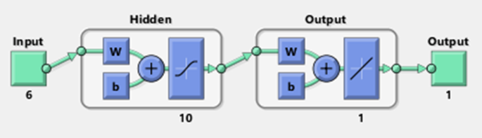
Selected neural network architecture


Figure 17a gives the performance graph for the CASIA version 1.0 showing the best performance validation 0.25312 at epoch 4, and Fig. 17b gives the performance graph for the CASIA version 4.0 showing the best performance validation 0.13209 at epoch 3. CASIA version 1.0 shows the best validation because the iris database does not include the specular reflections which CASIA version 4.0 has because of the specular reflections of the camera. The neural network is to generate a regression plot which emphasizes the association between the targets and the output of a network. If there is perfect training, the target and the network output will be precisely equal, but this relationship is hardly perfect in practice.

Performance graph showing the best validation at a Epoch 4 for CASIA version 1.0 database, b epoch 3 for CASIA version 4.0 database
The error histogram of the trained neural network for the training, validation and testing is shown by Fig. 18 and implies that the data fitting errors are uniformly distributed around zero within a reasonable range. Figure 18a gives the error histogram for the CASIA version 1.0 iris database, and Fig. 18b gives the error histogram for the CASIA version 4.0 iris database.

Error histogram plot for a CASIA version 1.0, b CASIA version 4.0
There are three plots of regression representing training, validation and testing. The perfect result output equal to target is symbolized by the dashed line, and the best fit linear regression line between the target and the output is shown in Fig. 19 by the solid line. The regression plots for the CASIA version 1.0 iris database are shown in Fig. 19a, and the regression plots for the CASIA version 4.0 iris database are shown in Fig. 19b. If the value of R is near to zero, then there is no linear relationship between the targets, but in case R is equal to one, then there is an exact correlation between the target and the outputs. The training data of our result direct a good fit. When the value of R is grander than 0.9, our succeeding stage would be to inspect whether there is a condition of extrapolation then the training set should be included in the dataset or the extrapolation then the superfluous data should be collected to be included in the test set. The accuracy achieved with CASIA version 1.0 is acceptable with an R value of 0.90433 which is very close to the ideal value of unity.

Regression plots for different values of R for a CASIA version 1.0 and CASIA version 4.0
Table 1 describes the performance of different methodologies for CASIA version 1.0 and CASIA version 4.0 iris databases in recognition of iris. It shows the recognition rates and average time taken by different methodologies.
Figure 20 shows the graph of the recognition rates of the methodologies used till date for the iris database version 1.0 and iris database version 4.0. It is clearly seen form the graph that this technique has outperformed the already existing techniques in the matching process and the computational effectiveness for the iris database version 1.0. Our proposed method has the recognition rates of 95% and 97% for the feed-forward neural network and radial basis function neural network, respectively, for CASIA version 1.0 and recognition rates of 94% and 95% for the feed-forward neural network and radial basis function neural network, respectively, for CASIA version 4.0.

Graph shows the recognition rates of the methods used
Figure 21 shows the graph of the average rates of the methodologies for the iris database version 1.0 and iris database version 4.0. It is clearly seen from the graph that the iris database version 1.0 and iris database version 4.0 take the less time. Our proposed method has the average time of 20 s and 10 s for the feed-forward neural network and radial basis function neural network, respectively, for CASIA version 1.0 and the average time 23 s and 15 s for the feed-forward neural network and radial basis function neural network, respectively, for CASIA version 4.0.

Graph shows the average time of the methods used
Table 2 shows the comparison of recognition rates when the proposed algorithm is performed on CASIA version 1.0 and on CASIA version 4.0 databases. The results are excellent for CASIA version 1.0 iris image database than those for CASIA version 4.0 iris databases. Therefore, the proposed methodology is proficient for the verification and identification.
6 Conclusion
Biometric iris recognition is an emerging field of interest and is needed in many areas. The iris has a data-rich physical and unique structure which is why it is considered as one of the robust ways to identify an individual. In this paper, a novel and efficient approach for iris recognition system using RBFNN is presented on CASIA version 1.0 and CASIA version 4.0 iris databases. The iris characteristics enhance its suitability in the automatic identification which includes: comfort of image registration at some distance, natural protection from external environment, surgical impossibilities without loss of vision. The application of iris recognition system has been seen in various areas of life such as crime detection, airport, business application, banks and industries.
The iris segmentation uses an integro-differential operator for the localization of iris and pupil boundaries, circular Hough transform for pupil circle detection. Iris normalization uses Daugman’s rubber sheet model and feature extraction by 1D Gabor filter since it includes the most supreme areas of the iris pattern and hence high recognition rate and reduced computation time is achieved. Classification is applied on finally extracted features. FNN and RBFNN are used as classifiers and give an accuracy of 95% and 97%, respectively, when compared to other methodologies. When worked on CASIA version 1.0 iris database, complexity and computational time are reduced as compared to other existing techniques. The methodology worked impeccably on CASIA version 1.0 in addition to CASIA version 4.0. In the future, an improved system can be accessible by investigating with the proposed iris recognition system under different constraints and environments.
References
Abhyankar A, Hornak L, Schuckers S (2005) Off-angle iris recognition using bi-orthogonal wavelet network system. In: Fourth IEEE workshop on automatic identification advanced technologies, 2005. IEEE, Washington, pp 239–244
Abiyev RH, Altunkaya K (2008) Personal iris recognition using neural network. Int J Secur Appl 2(2):41–50
Basit A, Javed MY, Anjum MA (2005) Biometric-enabled authentication machines: a survey of open-set real-world applications. WEC 2:24–26
Boles WW, Boashash B (1998) A human identification technique using images of the iris and wavelet transform. IEEE Trans Signal Process 46(4):1185–1188
Chawla S, Oberoi A (2011) A robust algorithm for iris segmentation and normalization using hough transform. Glob J Bus Manag Inf Technol 1(2):69–76
Chen X (2017) An effective synchronization clustering algorithm. Appl Intell 46(1):135–157
Cho DH, Park KR, Rhee DW (2005) Real-time iris localization for iris recognition in cellular phone. In: Sixth international conference on software engineering, artificial intelligence, networking and parallel/distributed computing, 2005 and first ACIS international workshop on self-assembling wireless networks. SNPD/SAWN 2005. IEEE, Washington, pp 254–259
Daouk CH, El-Esber LA, Kammoun FD, Al Alaoui MA (2002) Iris recognition. In: IEEE ISSPIT, pp 558–562
Daugman J (1992) High confidence personal identification by rapid video analysis of iris texture. In: International Carnahan conference on security technology, 1992 Crime countermeasures, proceedings. Institute of electrical and electronics engineers. IEEE, Washington, pp 50–60
Daugman JG (1993) High confidence visual recognition of persons by a test of statistical independence. IEEE Trans Pattern Anal Mach Intell 15(11):1148–1161
Daugman JG (1994) U.S. Patent No. 5,291,560. Washington, DC: U.S. Patent and Trademark Office. In: Jain A, Bolle R, Pankanti S (eds) Biometrics: personal identification in a networked society. Kluwer, Norwell
Daugman J (2001) Statistical richness of visual phase information: update on recognizing persons by iris patterns. Int J Comput Vis 45(1):25–38
Daugman J (2004) How iris recognition works. IEEE Trans Circuits Syst Video Technol 14(1):21–30
Daugman J (2007) New methods in iris recognition. IEEE Trans Syst Man Cybern Part B Cybern 37(5):1167–1175
Daugman J (2016) Information theory and the iris code. IEEE Trans Inf Forensics Secur 11(2):400–409
Eastwood SC, Shmerko VP, Yanushkevich SN, Drahansky M, Gorodnichy DO (2016) Biometric-enabled authentication machines: a survey of open-set real-world applications. IEEE Trans Hum Mach Syst 46(2):231–242
Galbally J, Marcel S, Fierrez J (2014) Image quality assessment for fake biometric detection: application to iris, fingerprints, and face recognition. IEEE Trans Image Process 23(2):710–724
Gupta K, Gupta R (2014) Iris recognition system for smart environments. In: 2014 international conference on data mining and intelligent computing (ICDMIC). IEEE, Washington, pp 1–6
Gupta R, Gupta K (2016) Iris recognition using templates fusion with weighted majority voting. Int J Image Data Fus 7(4):325–338
Haddouch K, Elmoutaoukil K, Ettaouil M (2016) Solving the weighted constraint satisfaction problems via the neural network approach. IJIMAI 4(1):56–60
Hu Y, Sirlantzis K, Howells G (2017) Optimal generation of iris codes for iris recognition. IEEE Trans Inf Forensics Secur 12(1):157–171
Hurtado MF, Langreo MH, De Miguel PM, Villanueva VD (2010) Biometry, the safe key. Int J Interact Multimed Artif Intell 1(3):33–37
Jain AK, Ross A, Prabhakar S (2004) An introduction to biometric recognition. IEEE Trans Circuits Syst Video Technol 14(1):4–20
Kushwaha P, Welekar RR (2016) Feature selection for image retrieval based on genetic algorithm. IJIMAI 4(2):16–21
Kyaw KSS (2009) Iris recognition system using statistical features for biometric identification. In: 2009 international conference on electronic computer technology. IEEE, Washington, pp 554–556
Liu Y, Nie L, Liu L, Rosenblum DS (2016) From action to activity: sensor-based activity recognition. Neurocomputing 181:108–115
López FRJ, Beainy CEP, Mendez OEU (2013) Biometric iris recognition using Hough transform. In: 2013 XVIII symposium of image, signal processing, and artificial vision (STSIVA). IEEE, Washington, pp 1–6
Ma L, Tan T, Wang Y, Zhang D (2004) Efficient iris recognition by characterizing key local variations. IEEE Trans Image Process 13(6):739–750
Masek L (2003) Recognition of human iris patterns for biometric identification, vol 26. Techreport. http://www.csse.uwa.edu.au/~pk/studentprojects/libor
Mock K, Hoanca B, Weaver J, Milton M (2012) Real-time continuous iris recognition for authentication using an eye tracker. In: Proceedings of the 2012 ACM conference on computer and communications security. ACM, New York, pp 1007–1009
Nguyen Thanh K, Fookes CB, Sridharan S (2010) Fusing shrinking and expanding active contour models for robust IRIS segmentation. In: Proceedings of 10th international conference on information science, signal processing and their applications. IEEE, Washington, pp 185–188
Njikam ANS, Zhao H (2016) A novel activation function for multilayer feed-forward neural networks. Appl Intell 45(1):75–82
Poursaberi A, Yanushkevich S, Gavrilova M, Shmerko V, Wang PSP (2013) Situational awareness through biometrics. IEEE Comput Spec Issue Cut Edge Res Vis 46(5):102–104
Punyani P, Gupta R (2015) Iris recognition system using morphology and sequential addition-based grouping. In: 2015 international conference on futuristic trends on computational analysis and knowledge management (ABLAZE). IEEE, Washington, pp 159–164
Roh MC, Fazli S, Lee SW (2016) Selective temporal filtering and its application to hand gesture recognition. Appl Intell 45(2):255–264
Schlett T, Rathgeb C, Busch C (2018) Multi-spectral iris segmentation in visible wavelengths. In: 2018 international conference on biometrics (ICB). IEEE, Washington
Sharma K, Monga H (2014) Efficient biometric iris recognition using hough transform with secret key. Int J Adv Res Comput Sci Softw Eng 4(7):104–109
Shylaja SS, Murthy KB, Natarajan S, Muthuraj R, Ajay S (2011) Feed forward neural network based eye localization and recognition using Hough transform. IJACSA Editorial
Sundaram RM, Dhara BC (2011) Neural network-based Iris recognition system using Haralick features. In: 2011 3rd international conference on electronics computer technology (ICECT), vol 3. IEEE, Washington, pp 19–23
Tripathi BK (2017) On the complex domain, deep machine learning for face recognition. Appl Intell 47:382–396
Vatsa M, Singh R, Noore A (2007) Integrating image quality in 2ν-SVM biometric match score fusion. Int J Neural Syst 17(05):343–351
Wang Y, Tan T, Jain AK (2003) Combining face and iris biometrics for identity verification. In: International conference on audio-and video-based biometric person authentication. Springer, Berlin, pp 805–813
Wildes RP, Asmuth JC, Green GL, Hsu SC, Kolczynski RJ, Matey JR, MBride SE (1994) A system for automated iris recognition. In: Proceedings of the applications of computer vision, 1994
Xiao Q (2007) Technology review-biometrics-technology, application, challenge, and computational intelligence solutions. IEEE Comput Intell Mag 2(2):5–25
Yu Q, Luo Y, Chen C, Ding X (2016) Outlier-eliminated k-means clustering algorithm based on differential privacy preservation. Appl Intell 45(4):1179–1191
Zhu Y, Tan T, Wang Y (2000) Biometric personal identification based on iris patterns. In: ICPR. IEEE, p 2801
Author information
Authors and Affiliations
Corresponding author
Ethics declarations
Conflict of interest
The authors declare that they have no conflict of interest.
Ethical approval
This article does not contain any studies with human participants or animals performed by any of the authors.
Additional information
Communicated by V. Loia.
Publisher’s Note
Springer Nature remains neutral with regard to jurisdictional claims in published maps and institutional affiliations.
Rights and permissions
About this article

Cite this article
Dua, M., Gupta, R., Khari, M. et al. Biometric iris recognition using radial basis function neural network. Soft Comput 23, 11801–11815 (2019). https://doi.org/10.1007/s00500-018-03731-4
Published:
Issue Date:
DOI: https://doi.org/10.1007/s00500-018-03731-4