A hybrid interval displacement forecasting model for reservoir colluvial landslides with step-like deformation characteristics considering dynamic switching of deformation states

Abstract

Constructing an accurate and dependable displacement forecasting model is a prerequisite for realizing effective early warning systems of landslide disasters. To overcome the drawbacks of previous displacement prediction models for landslides with step-like deformation characteristics, such as the low prediction accuracy of the mutational displacements and the unclear reliability of the prediction results, we propose a novel hybrid interval forecasting model. This model consists of four parts. First, clustering by fast search and find of density peaks is implemented to distinguish the deformation states of the landslide. Second, the ensemble classifier based on the random forest algorithm is established to identify the deformation states. Third, based on the wild bootstrap, kernel extreme learning machine, and back propagation neural network approaches, the ensemble regressors under different deformation states are built. Finally, by combining the ensemble classifier and ensemble regressors, an interval prediction framework is constructed to realize the dynamic interval prediction of landslide displacement. Taking the Baishuihe landslide as an example, the datasets of three monitoring sites from June 2006 to December 2016 are used to verify the accuracy and reliability of the proposed model. The results show that the proposed model can effectively improve the prediction accuracy of mutational displacements, with the root mean square errors of 28.19 mm, 14.21 mm, and 34.44 mm and the R-squares of 0.9827, 0.9955, and 0.9903, respectively. Moreover, the reliability of the prediction results obtained using this model can be expressed in the flexible prediction intervals (PIs) under different deformation states. The coverage width-based criteria of PIs at 90% nominal confidence are 140.38 mm, 86.61 mm, and 173.68 mm, respectively. In conclusion, the proposed model provides a good basis for developing early warning systems for landslides with step-like deformation characteristics.

1 Introduction

Landslides are one of the most common and significant geological hazards in nature, resulting in thousands of casualties and billions of dollars in losses every year worldwide (Gorsevski et al. 2003). Due to its unique geological, climatical, and environmental conditions, the Three Gorges Reservoir (TGR) area has always been a high-incidence area for landslide hazards (Tang et al. 2019). Since the impoundment of the TGR in 2003, under the coupled impact of continuous heavy precipitation and periodic reservoir water level variations, the cumulative displacements of some reservoir colluvial landslides in this area have shown similar periodic and extreme changes every year (Du et al. 2013; Lian et al. 2014a, b). These extreme changes in monitored displacements of landslides pose severe threats to the lives and property of residents. Therefore, in recent years, continuous efforts have been devoted to developing monitoring technologies and theoretical methods to realize the accurate and reliable early warning of landslides (Li et al. 2014; Intrieri et al. 2019; Tang et al. 2019), especially for the reservoir colluvial landslides whose deformations exhibit significant step-like characteristics (Miao et al. 2018; Liao et al. 2020).

To date, most prediction models for landslides with step-like deformation characteristics have been built based on the theory of time series analysis (Lian et al. 2014a; Zhou et al. 2016; Wen et al. 2017). In these models, various signal decomposition methods are first used to decompose the cumulative displacement into different components: the trend, periodic, and random terms. Subsequently, some novel mathematical statistics or machine learning models have been applied as prediction models. The well-trained prediction models of them are used to predict each displacement component. Then, the cumulative displacement is predicted by superimposing the prediction result of each component. So far, with the continuous development of signal decomposition technologies and machine learning models, the performance of this kind of model has been gradually and significantly improved (Lian et al. 2013; Ren et al. 2015; Cai et al. 2016; Huang et al. 2017; Zhu et al. 2018; Zou et al. 2020).

Nevertheless, the prediction models mentioned above are all point prediction models, and it is complicated to express the reliability of their prediction results quantitatively. Therefore, to more accurately quantify the reliability of the prediction results and provide more practical information for the risk decision, some novel prediction models, namely, interval prediction models, have been proposed recently. For example, Lian et al. (2016) proposed an interval prediction model of landslide displacement based on a novel neural network model with high prediction accuracy, strong generalization ability, and good robustness. Ma et al. (2018) used a hybrid approach based on the bootstrap, extreme learning machine (ELM), and artificial neural network (ANN) approaches to quantify the associated uncertainties in landslide displacement forecasting. Wang et al. (2019) proposed a hybrid model based on double exponential smoothing and lower and upper bound estimation to construct the prediction intervals (PIs) of landslide displacement.

However, for landslides with step-like deformation characteristics, the variations in their deformation rates in different periods significantly differ. If the interval prediction models mentioned above are directly applied to predict the displacement interval of these landslides, the data corresponding to a period of a sharp increase in landslide displacement might be incorrectly marked as outlier data in the training process (Lian et al. 2018). This issue is bound to lead to the underfitting of prediction results, meaning that the prediction results of these sharply increasing displacement points would always significantly underestimate their actual values. Thus, it is essential to consider the influence of the dynamic switching among different deformation states on the performance of interval prediction models for landslides with step-like deformation characteristics.

In this paper, based on the three-stage evolution model of progressive landslides, the deformation responses of landslides with step-like deformation characteristics under the coupling impacts of complex external inducing factors were analyzed first. Then, according to the analysis results, the dynamic switching between two different deformation states observed in the evolution of landslides with step-like deformation characteristics was defined. Finally, a novel hybrid interval prediction model considering the dynamic switching of deformation states was proposed. This proposed model included the clustering by fast search and find of density peaks (CFSFDP), engineering geology analogy (EGA), adaptive synthetic sampling (ADASYN), random forest (RF), wild bootstrap (WB), kernel extreme learning machine (KELM), and back-propagation neural network (BPNN) approaches. The Baishuihe landslide, a typical reservoir colluvial landslide with step-like deformation characteristics in the TGR area, was taken as a case study to explore the effectiveness, accuracy, and reliability of the proposed model. Two core issues about improving the performance of this model were discussed in detail within the performance comparison of models. The obtained results can be useful for the displacement prediction of similar reservoir colluvial landslides with step-like deformation characteristics in the TGR area.

2 Theoretical basis, methodology, and evaluation index

2.1 Evolution of landslides with step-like deformation characteristics

Many rock and soil creep tests and monitoring data show that under the influence of gravity, the deformation evolution of progressive landslides can be divided into three stages (Fig. 1a): the primary (or decelerating or transient) creep stage, secondary (or steady-state) creep stage, and tertiary (or accelerating) creep stage (Xu et al. 2015; Intrieri et al. 2019). However, in nature, landslides are disturbed by various external factors, thus resulting in some inevitable fluctuations or step-like growths of the displacement–time monitoring curves. Therefore, for actual progressive landslides, their displacement–time curves follow the three-stage creep evolution law on the whole but exhibit unique variation characteristics locally (Xu et al. 2015). For example, due to the coupling impacts of the continuous evolution of internal geological conditions and the dynamic change in external factors (mainly periodic heavy precipitation), the Xintan landslide, a typical ancient colluvial landslide in the TGR area, underwent the whole evolution of progressive landslides from November 1977 to June 1985 (He et al. 2010). As shown in Fig. 1b, the displacements of the landslide underwent several sharp increases to different extents from its secondary creep stage to ultimate failure. Similar variations in displacements have been reported in some other reservoir colluvial landslides in the TGR area, such as the Bazimen landslide (Zhou et al. 2016), Shuping landslide (Wang et al. 2020), and Baijiabao landslide (Yao et al. 2019). For the convenience of expression, this type of landslide is usually defined as a step-like landslide (Miao et al. 2018), in which the step-like shape refers to the step-like increase in the landslide displacements rather than the step-like shape of the landslide topography.

Fig. 1

a Three-stage evolution law of progressive landslides; b displacement monitoring curves and monthly precipitation of the Xintan landslide

For step-like landslides, without violating the three-stage evolution law, two alternating deformation states (i.e., stable and mutation states) caused by the strong influence of external periodic factors are observed in the secondary and tertiary stages. The stable state is defined as the deformation state in which the increase in displacement is relatively stable. The mutation state is defined as the deformation state in which the displacement increases sharply. Moreover, it should be emphasized that these two states cannot alternate forever. Under the action of complex external periodic factors, when the landslide finally enters the tertiary creep stage and is on the verge of instability, the landslide must be in the mutation state. Thus, considering the characteristics of the machine learning methods, how to correctly understand the dynamic switching law between these two deformation states is the significant precondition of building the displacement prediction model for step-like landslides.

2.2 Displacement interval prediction model considering the dynamic switching of deformation states

2.2.1 Division of landslide deformation states

The division of the deformation states for step-like landslides is essentially a clustering process. In this process, the characteristic parameters of landslide deformation, such as the cumulative displacement increments, tangent angles, velocities, and accelerations, are clustered into two different classes that correspond to the different deformation states of step-like landslides. The K-means algorithm is the most widely used approach in the division of landslide deformation states. However, due to inherent defects, such as the strong dependence on the initial center value, ease of falling into a local optimum, and reliance on experience to determine the number of optimal classes, the clustering effect of the K-means algorithm is sometimes limited.

The CFSFDP algorithm is a novel density-based clustering algorithm (Rodriguez and Laio 2014). This algorithm can identify the cluster centers of samples by finding the density peaks, which makes it possible to cluster the high-dimensional datasets with arbitrary shapes effectively. Only one parameter, namely, the truncation distance $d_{c}$, is needed in the clustering process, and the clustering results are insensitive to the parameter setting. Therefore, the CFSFDP algorithm was implemented in this study to realize the division of the deformation states for the step-like landslide.

2.2.2 Identification of landslide deformation states

Due to the unique characteristics of their evolutions, step-like landslides usually correspond to significant potential instability risks. Thus, identifying their deformation states is critical to prevent and reduce the landslide disaster risks. The identification of landslide deformation states is essentially a typical classification process. In this process, the corresponding classification model is first established by mining the nonlinear relationship between various external factors and different deformation states. After that, the established model is used to accurately identify the deformation state of landslides during the dynamic switching process of deformation states.

The RF algorithm is an ensemble learning method that implements prediction by training a large number of classification and regression trees (Breiman 2001). Compared with traditional classification algorithms, such as the support vector machine (SVM), extreme learning machine (ELM), and decision tree algorithms, this algorithm introduces two random sampling processes in the selection of training samples and input factors (Zhou et al. 2019). These two processes effectively avoid the occurrence of overfitting. Thus, the RF algorithm clearly meets the basic requirements of landslide deformation state identification.

The uneven distribution of data is a widespread problem in classification research. In the deformation parameters of step-like landslides, the ratio of stable state samples to mutation state samples is higher than 3:1. Unfortunately, most of the traditional classification algorithms, including the RF algorithm, assume that the distribution of data is balanced. When the proportion of the majority class samples is too high, it inevitably leads to the neglect of the minority class samples. In some extreme cases, the minority class samples are ignored because they are misidentified as outliers of the majority class samples. To accurately identify the deformation state of step-like landslides, the accuracy and reliability of the selected algorithm should be considered, and the imbalance problem of training data should be addressed effectively.

The ADASYN approach is a novel data synthesis method based on the classical synthetic minority oversampling technique (SMOTE) (He et al. 2008). This approach can adaptively synthesize the appropriate number of minority class samples according to the distribution characteristics of the training samples. However, we cannot blindly and directly use this type of resampling technique to address the practical imbalance problem that needs to be solved. Therefore, to obtain more useful information with definite physical meaning and reduce the risk of changing the data authenticity, we proposed a modified comprehensive method based on the engineering geology analogy (EGA) method and the ADASYN approach. The specific steps of this method were as follows:

• 1. The similarity between the research object and other actual step-like landslides in terms of the external factors, geological conditions, deformation evolution characteristics, and deformation responses were first analyzed by applying the EGA method. One or more cases that were most similar to the research object were selected from these step-like landslides. Afterward, supplementary samples of the mutation state were obtained from these cases.

• 2. If the number of these supplementary samples was insufficient to make the distribution of the training samples completely balanced, a certain number of mutation state samples were appropriately synthesized by applying the ADASYN method based on the mutation state samples of the research object and that of analogous landslide examples.

If there are several monitoring sites on the research object, the supplement samples of the mutation state can also be selected according to the similarity of the displacement versus time curves between the different monitoring sites. In this study, the monitoring sites ZG93, ZG118, and XD01 are all located in the warning zone of the Baishuihe landslide. This means that these three monitoring sites have similar geological and geomorphological conditions, deformation influencing factors, and historical deformation characteristics. Thus, the mutation state samples of monitoring sites ZG93 and ZG118 can be used as supplementary samples of monitoring site XD01, and vice versa. On this basis, an RF-based ensemble classifier was established to realize the accurate identification of the deformation states.

2.2.3 Interval prediction of landslide displacements under different deformation states

As described in Sect. 2.1, whether the deformation state changes abruptly is not the essential condition for the catastrophe of step-like landslides. If we want to achieve the accurate early warning of step-like landslides, it is imperative to predict the displacement of these landslides accurately. However, due to the coupling effects of various uncertainties in landslide geological models, prediction models, input data, and other factors (Wu et al. 2014), any prediction of landslides cannot be wholly accurate and dependable. For the traditional point prediction models, only the displacement is used as the prediction object. This seriously limits the quantitative characterization of the reliability of its own final prediction results. To address this issue properly, interval prediction models were recently proposed to evaluate the epistemic uncertainties associated with landslide displacement prediction (Ma et al. 2018). Thus, to improve the credibility and practicality of the prediction results, it is indispensable to introduce the idea of interval prediction into the regression of landslide displacements.

The WB-KELM-BPNN model is an integrated interval forecasting model based on the KELM model (Huang et al. 2011) and was fully adopted in the interval predictions of landslide displacement under different deformation states in this study. The calculation process of the model is shown in Fig. 2. Khosravi et al. (2011) introduced the construction of the bootstrap-based method similar to the WB-KELM-BPNN model, and more information about the bootstrap-based method can be found in their study. For the convenience of description and comparison, in the latter part of the study, the proposed hybrid model is called the modified model, while the WB-KELM-BPNN model is called the unmodified model.

Fig. 2

Flowchart of the WB-KELM-BPNN model

2.2.4 Framework of the hybrid interval prediction model for landslide displacement

The primary process of the proposed hybrid model is shown in Fig. 3. It mainly includes the following four steps: (1) Division of deformation states; (2) Identification of deformation states; (3) Construction of the interval prediction model for landslide displacements under different deformation states; and (4) Landslide displacement interval prediction considering the dynamic switching of deformation states. The specific calculation process is as follows:

Fig. 3

Flowchart of the proposed interval prediction hybrid model

• 1. Division of deformation states

  • 1. The monthly increment of landslide displacement and its corresponding tangential angle were obtained as follows:

    $$\Delta t_{i} = t_{i} - t_{i - 1} ,\quad \, i = 1,2, \ldots ,N$$

    (1)
    $$\varphi \left( {\Delta t_{i} } \right) = \text{actan} \left( {\frac{{\Delta t_{i} }}{\Delta T}} \right)*\frac{\pi }{180}$$

    (2)

    where $t_{i}$ is the cumulative landslide displacement, $\Delta t_{i}$ is the monthly increment of $t_{i}$, $\varphi \left( {\Delta t_{i} } \right)$ is the tangential angle of $\Delta t_{i}$, and $\Delta T$ is the sampling period of landslide displacement. In this paper, we set $\Delta T = 30\,{\text{days}}$.

  • 2. The CFSFDP algorithm was used to cluster the $\Delta t_{i}$ and $\varphi \left( {\Delta t_{i} } \right)$ comprehensively. According to clustering results, the landslide deformation state $C_{i}$ was divided into the stable state C_I and the mutation state C_II.

  • 3. A new dataset $D^{C}$ was constructed for classification, and $D^{C} = D_{train}^{C} \cup D_{test}^{C} = \left\{ {\left( {X_{i} ,c_{i} } \right)} \right\}_{i = 1}^{{N_{train + test} }}$. Wherein $X_{i}$ is the input factors, and $\left\{ {X_{i} } \right\}_{i = 1}^{{N_{train} + N_{test} }} = X_{train} \cup X_{test} = \left[ {x_{i1} ,x_{i2} , \ldots ,x_{iM} } \right]^{\text{T}} \in R^{M}.$ $c_{i}$ is the class label of different landslide deformation states, and $\left\{ {c_{i} } \right\}_{i = 1}^{{N_{train} + N_{test} }} = c_{train} \cup c_{test}$. $c_{i}$ can be expressed as follows:

    $$c_{i} = \left\{ {\begin{array}{*{20}c} 1 & {C_{i} \in C_{\text{I}} } \\ { - 1} & {C_{i} \in C_{\text{II}} } \\ \end{array} } \right.$$

    (3)

• 2. Identification of deformation states

  • 1. $D_{train}^{C}$ was divided into two sub-datasets according to the following equations:

    $$D_{{train\,{\text{I}}}}^{C} = \left\{ {\left( {X_{i} ,c_{i} } \right)|X_{i} \in X_{train} ,C_{i} \in C_{\text{I}} } \right\}_{i = 1}^{{N_{{train\,{\text{I}}}} }}$$

    (4)
    $$D_{{train\,{\text{II}}}}^{C} = \left\{ {\left( {X_{i} ,c_{i} } \right)|X_{i} \in X_{train} ,C_{i} \in C_{\text{II}} } \right\}_{i = 1}^{{N_{{train\,{\text{II}}}} }}$$

    (5)

    where $D_{{train\,{\text{I}}}}^{C}$ is the training sub-datasets for the classification of the stable state, and $D_{{train\,{\text{II}}}}^{C}$ is the training sub-datasets for the classification of the mutation state.

  • 2. The hybrid model composed of EGA and ADASYN was employed to obtain supplement samples of $D_{{train\,{\text{I}}}}^{C}$. After that, the new mutation state sub-dataset $D_{{train\,{\text{II}}}}^{C *}$ was built to balance the sample distribution of training data.

  • 3. Based on $D_{{train\,{\text{I}}}}^{C}$ and $D_{{train\,{\text{II}}}}^{C *}$, an ensemble classifier composed of many classification and regression trees by using the RF algorithm was built.

  • 4. Using the ensemble classifier to predict $c_{i}$, the predicted results were as follows:

    $$\left\{ {\hat{c}_{i} } \right\}_{i = 1}^{{N_{train} + N_{test} }} = \hat{c}_{train} \cup \hat{c}_{test}$$

    (6)

  • 5. According to the classification prediction results and Eq. (3), the identification results were obtained as follows:

    $$\left\{ {\hat{C}_{i} } \right\}_{i = 1}^{{N_{train} + N_{test} }} = \hat{C}_{train} \cup \hat{C}_{test}$$

    (7)

• 3. Construction of the interval prediction model for landslide displacement under different deformation states

  • 1. A new dataset $D^{R}$ was constructed for regression, and $D^{R} = D_{train}^{R} \cup D_{test}^{R} = \left\{ {\left( {X_{i} ,t_{i} } \right)} \right\}_{i = 1}^{{N_{train + test} }}$.

  • 2. According to the identification results $\hat{C}_{train}$, $D_{train}^{R}$ was divided into two sub-datasets according to the following equations:

    $$D_{{train\,{\text{I}}}}^{R} = \left\{ {\left( {X_{i} ,t_{i} } \right)|X_{i} \in X_{train} ,\hat{C}_{i} \in C_{\text{I}} } \right\}_{i = 1}^{{N_{{train\,{\text{I}}}} }}$$

    (8)
    $$D_{{train\,{\text{II}}}}^{R} = \left\{ {\left( {X_{i} ,t_{i} } \right)|X_{i} \in X_{train} ,\hat{C}_{i} \in C_{\text{II}} } \right\}_{i = 1}^{{N_{{train\,{\text{II}}}} }}$$

    (9)

    where $D_{{train\,{\text{I}}}}^{R}$ is the training sub-datasets for the regression of the stable state, and $D_{{train\,{\text{II}}}}^{R}$ is the training sub-datasets for the regression of the mutation state.

  • 3. By using the WB method, random resampling with replacement was conducted on $D_{{train\,{\text{I}}}}^{R}$ and $D_{{train\,{\text{II}}}}^{R}$ separately. After $B$ times of resampling, $B$ bootstrap sub-datasets of stable deformation state $D_{1}^{\text{I}} ,D_{2}^{\text{I}} , \ldots ,D_{B}^{\text{I}}$ and B bootstrap sub-datasets of mutation deformation state $D_{1}^{\text{II}} ,D_{2}^{\text{II}} , \ldots ,D_{B}^{\text{II}}$ were generated.

  • 4. Based on $D_{{train\,{\text{I}}}}^{R}$ and $D_{{train\,{\text{II}}}}^{R}$, two different KELM models were established separately. Then, the Grey Wolf Optimization (GWO) algorithm proposed by Mirjalili et al. (2014) was used to optimize the hyperparameters of KELM models.

  • 5. According to the sub-datasets and the optimized hyperparameters, two sets of different KELM-BPNN integration models were trained separately. Each integration model consists of $B$ KELM models and a BPNN model, wherein the BPNN models were respectively trained according to the squared residuals (i.e., $r_{{train\,{\text{I}}}}^{2}$ and $r_{{train\,{\text{II}}}}^{2}$) of the predicted means obtained from two sets of $B$ KELM models.

• 4. Landslide displacement interval prediction considering the dynamic switching of deformation states

  • 1. The integration models were used to forecast the landslide displacements. The predicted results were expressed as $\left\{ {\hat{y}_{l}^{\text{I}} \left( {x_{i} } \right)} \right\}_{l = 1}^{B}$ and $\left\{ {\hat{y}_{l}^{\text{II}} \left( {x_{i} } \right)} \right\}_{l = 1}^{B}$, and $\hat{y}\left( {x_{i} } \right) = \left\{ {\hat{y}_{l}^{\text{I}} \left( {x_{i} } \right)} \right\}_{l = 1}^{B} \cup \left\{ {\hat{y}_{l}^{\text{II}} \left( {x_{i} } \right)} \right\}_{l = 1}^{B}$.

  • 2. The predicted landslide displacements were assumed to be unbiased. The mean values of predicted landslide displacements and their variances (as known as the variance of the system error) were obtained according to the following equations:

    $$\hat{y}\left( {x_{i} } \right) = \hat{y}_{\text{I}} \left( {x_{i} } \right) \cup \hat{y}_{\text{II}} \left( {x_{i} } \right) = \frac{1}{B}\sum\limits_{l = 1}^{B} {\hat{y}_{l} \left( {x_{i} } \right)}$$

    (10)
    $$\sigma_{{\hat{y}}}^{2} \left( {x_{i} } \right) = \sigma_{{\hat{y}_{\text{I}} }}^{2} \left( {x_{i} } \right) \cup \sigma_{{\hat{y}_{\text{II}} }}^{2} \left( {x_{i} } \right) = \frac{1}{B - 1}\sum\limits_{l = 1} {\left[ {\hat{y}_{l} \left( {x_{i} } \right) - \hat{y}\left( {x_{i} } \right)} \right]^{2} }$$

    (11)

    where $\hat{y}_{\text{I}} \left( {x_{i} } \right)$ is the mean value of predicted landslide displacement under the stable deformation state, $\hat{y}_{\text{II}} \left( {x_{i} } \right)$ is the mean value of predicted landslide displacement under the mutation deformation state, $\sigma_{{\hat{y}_{\text{I}} }}^{2} \left( {x_{i} } \right)$ is the variance corresponding to $\hat{y}_{\text{I}} \left( {x_{i} } \right)$, and $\sigma_{{\hat{y}_{\text{II}} }}^{2} \left( {x_{i} } \right)$ is the variance corresponding to $\hat{y}_{\text{II}} \left( {x_{i} } \right)$.

  • 3. For constructing the PI of the landslide displacement under different deformation states, after determining the variance of systematic error, the variances of random error (i.e., $\sigma_{{\hat{y}_{\text{I}} }}^{2} \left( {x_{i} } \right)$ and $\sigma_{{\hat{y}_{\text{II}} }}^{2} \left( {x_{i} } \right)$) also need to be estimated according to the following equations:

    $$\sigma_{\varepsilon }^{2} \left( {x_{i} } \right) = \sigma_{{\varepsilon_{\text{I}} }}^{2} \left( {x_{i} } \right) \cup \sigma_{{\varepsilon_{\text{II}} }}^{2} \left( {x_{i} } \right)\,\sim\,E\left\{ {\left( {y\left( {x_{i} } \right) - \hat{y}\left( {x_{i} } \right)} \right)^{2} } \right\} - \sigma_{{\tilde{y}}}^{2} \left( {x_{i} } \right)$$

    (12)

    For realizing the prediction of $\sigma_{{\varepsilon_{\text{I}} }}^{2} \left( {x_{i} } \right)$ and $\sigma_{{\varepsilon_{\text{II}} }}^{2} \left( {x_{i} } \right)$, it is necessary to construct two new sub-datasets (i.e., $D_{{r_{\text{I}}^{2} }}$ and $D_{{r_{\text{II}}^{2} }}$) of corresponding squared residuals $r_{{i\,{\text{I}}}}^{2}$ and $r_{{i\,{\text{II}}}}^{2}$. Then, the trained BPNN models in two different KELM-BPNN integration models were respectively used to achieve the prediction of random error variances. The $r_{{i\,{\text{I}}}}^{2}$, $r_{{i\,{\text{II}}}}^{2}$, $D_{{r_{\text{I}}^{2} }}$ and $D_{{r_{\text{II}}^{2} }}$ are defined as follows:

    $$r_{{i{\text{ I}}}}^{2} = r_{{train{\text{ I}}}}^{2} \cup r_{{test{\text{ I}}}}^{2} = \hbox{max} \left[ {\left( {t_{{i{\text{ I}}}} - \hat{y}_{\text{I}} } \right)^{2} - \sigma_{{\hat{y}_{\text{I}} }}^{2} ,0} \right]$$

    (13)
    $$r_{{i{\text{ II}}}}^{2} = r_{{train{\text{ II}}}}^{2} \cup r_{{test{\text{ II}}}}^{2} = \hbox{max} \left[ {\left( {t_{{i{\text{ II}}}} - \hat{y}_{\text{II}} } \right)^{2} - \sigma_{{\hat{y}_{\text{II}} }}^{2} ,0} \right]$$

    (14)
    $$D_{{r_{\text{I}}^{2} }} = D_{{r_{\text{I}}^{2} }}^{train} \cup D_{{r_{\text{I}}^{2} }}^{test} = \left\{ {\left( {X_{{i{\text{ I}}}} ,r_{{i{\text{ I}}}}^{2} } \right)} \right\}_{i = 1}^{{N_{train} + N_{test} }}$$

    (15)
    $$D_{{r_{\text{II}}^{2} }} = D_{{r_{\text{II}}^{2} }}^{train} \cup D_{{r_{\text{II}}^{2} }}^{test} = \left\{ {\left( {X_{{i{\text{ II}}}} ,r_{{i{\text{ II}}}}^{2} } \right)} \right\}_{i = 1}^{{N_{train} + N_{test} }}$$

    (16)

    where $r_{{i{\text{ I}}}}^{2}$ is the squared residual set of the stable state, $r_{{i{\text{ II}}}}^{2}$ is the square residual set of the mutation state, $D_{{r_{\text{I}}^{2} }}$ is the regression sub-dataset for the BPNN model under the stable state, and $D_{{r_{\text{II}}^{2} }}$ is the regression sub-dataset for the BPNN model under the mutation state. The $r_{{train{\text{ I}}}}^{2}$, $r_{{train{\text{ I}}}}^{2}$, $D_{{r_{\text{I}}^{2} }}^{train}$ and $D_{{r_{\text{II}}^{2} }}^{train}$ are generated during the training process of KELM-BPNN integration models.

• 4. The calculation results obtained in step (3) and step (4) were then reassembled according to the sequence of monitoring time. Then, the mean values of landslide displacement prediction were taken as the results of point estimation. Afterward, the interval estimation results of landslide displacement were constructed by:

  $$I_{t}^{\alpha } \left( {x_{i} } \right) = \left[ {L_{t}^{\alpha } \left( {x_{i} } \right),U_{t}^{\alpha } \left( {x_{i} } \right)} \right]$$

  (17)
  $$\sigma_{t}^{2} \left( {x_{i} } \right) = \sigma_{{\hat{y}}}^{2} \left( {x_{i} } \right) + \sigma_{\varepsilon }^{2} \left( {x_{i} } \right)$$

  (18)
  $$L_{t}^{\alpha } \left( {x_{i} } \right) = \hat{y}\left( {x_{i} } \right) - z_{1 - \alpha /2} \sqrt {\sigma_{t}^{2} \left( {x_{i} } \right)}$$

  (19)
  $$U_{t}^{\alpha } \left( {x_{i} } \right) = \hat{y}\left( {x_{i} } \right) + z_{1 - \alpha /2} \sqrt {\sigma_{t}^{2} \left( {x_{i} } \right)}$$

  (20)

  where $I_{t}^{\alpha } \left( {x_{i} } \right)$ is the displacement PI under the confidence level of $\left( {1 - \alpha } \right) \times 100\%$, $L_{t}^{\alpha } \left( {x_{i} } \right)$ is the lower limit of the PI $I_{t}^{\alpha } \left( {x_{i} } \right)$, $U_{t}^{\alpha } \left( {x_{i} } \right)$ is the upper limit of the PI $I_{t}^{\alpha } \left( {x_{i} } \right)$, $z_{1 - \alpha /2}$ is the quantile of the standard normal distribution, and $\sigma_{t}^{2} \left( {x_{i} } \right)$ is the variance of the total error.

2.3 Performance evaluation index of the prediction result

2.3.1 Clustering results of deformation state

The Silhouette Coefficient (SC) was used for evaluating the clustering effect of the deformation states. Its specific definition is as follows:

$$s\left( i \right) = \frac{b\left( i \right) - a\left( i \right)}{{\hbox{max} \{ a\left( i \right),b\left( i \right)\} }}$$

(21)

$$SC = \frac{1}{N}\sum\limits_{i = 1}^{N} {s\left( i \right)}$$

(22)

where $s\left( i \right)$ is the Silhouette Coefficient of the sample $i$, $a\left( i \right)$ is the average distance from the sample $i$ to other samples from the same cluster, $b\left( i \right)$ is the average distance from the sample $i$ to samples of other different clusters, and $SC$ is the mean Silhouette Coefficient for all samples. The range of $SC$ is [− 1,1]. The closer the $SC$ is to 1, and the better the clustering effect is.

2.3.2 Classification results of deformation state

Four different evaluation indexes of unbalanced data classification effects that are proposed based on the confusion matrix (Table 1) were used for the evaluating of the deformation state identification effect.

Table 1 Confusion matrix for performance evaluation

• 1. Overall accuracy (OA), as shown in Eq. (23), is the proportion of the number of samples with correct classification to the total number of samples.

  $$OA = \frac{TP + TN}{TP + FP + FN + TN}$$

  (23)

• 2. Sensitivity, as shown in Eq. (24), is the proportion of majority class samples with correct classification to the total number of majority class samples. It measures the classifier’s recognition ability for the majority class.

  $$Sensitivity = \frac{TP}{TP + FN}$$

  (24)

• 3. Specificity, as shown in Eq. (25), is the proportion of minority class samples with correct classification to the total number of minority class samples. It measures the classifier’s recognition ability for the minority class.

  $$Specificity = \frac{TN}{TN + FP}$$

  (25)

• 4. Geometric mean (G_mean), as shown in Eq. (26), refers to the average ability of the classifier to identify the majority class and the minority class correctly.

  $$G_{ - } mean{\mkern 1mu} {\mkern 1mu} = \sqrt {Sensitivity*Specificity}$$

  (26)

2.3.3 Regression results of landslide displacement

Root mean square error (RMSE) and R-square (R²) were used to evaluate the point prediction effects of models. The prediction interval coverage probability (PICP), mean prediction interval width (MPIW), and coverage width-based criterion (CWC) were applied to evaluate the interval prediction effects of models.

• 1. PICP, as shown in Eqs. (27) and (28), is the probability that the actual observation falls within the upper and lower bounds of the PI. It can be used to measure the reliability of the PI.

  $$PICP = \frac{1}{{N_{test} }}\sum\limits_{i = 1}^{{N_{test} }} {a_{i} }$$

  (27)
  $$a_{i} = \left\{ {\begin{array}{*{20}c} 1 & {t_{i} \in \left[ {L_{t}^{\alpha } \left( {X_{i} } \right),\,U_{t}^{\alpha } \left( {X_{i} } \right)} \right]} \\ 0 & {t_{i} \notin \left[ {L_{t}^{\alpha } \left( {X_{i} } \right),\,U_{t}^{\alpha } \left( {X_{i} } \right)} \right]{\mkern 1mu} } \\ \end{array} } \right.$$

  (28)

  where $N_{test}$ is the number of testing samples and $a_{i}$ is a Boolean variable.

• 2. MPIW, as shown in Eq. (29), is the average width between the upper and lower bounds of the PI under the significance level $\alpha$. It can be used to measure the clarity of the prediction results to avoid the PI being too full due to the blind pursuit of reliability.

  $$MPIW = \frac{1}{{N_{test} }}\sum\limits_{i = 1}^{{N_{test} }} {\left[ {U_{t}^{\alpha } \left( {X_{i} } \right) - L_{t}^{\alpha } \left( {X_{i} } \right)} \right]} .$$

  (29)

• 3. CWC, as shown in Eqs. (30) and (31), is a comprehensive index for evaluating the quality of PIs. It can be used to quantify the balance between the reliability and clarity of prediction results.

  $$CWC = MPIW\left( {1 + \gamma \cdot PICP \cdot e^{{ - \eta \left( {PICP - \mu } \right)}} } \right)$$

  (30)
  $$\gamma = \left\{ {\begin{array}{*{20}c} {0,} & {PICP \ge \mu } \\ {1,} & {PICP < \mu } \\ \end{array} } \right.$$

  (31)

  where $\gamma$ is a Boolean variable, $\eta$ is a penalty parameter, and $\mu$ is a constant equal to the confidence level $\left( {1 - \alpha } \right) \times 100\%$. In this study, we set $\eta = 50$.

3 Application to the Baishuihe landslide, TGR area, China

3.1 Geological conditions, movement history, and field monitoring

As shown in Fig. 4, the Baishuihe landslide is located on the right bank of the Yangtze River. This landslide is a large-scale ancient colluvial landslide with an average slope inclination of 30°, an average thickness of 30 m, and a volume of 1.26 × 10⁷ m³. The main sliding direction is 20° NE. The north–south and east–west lengths are 600 m and 700 m, respectively. The toe of the landslide extends to the riverbed of the Yangtze River. The bedrock ridge bounds the east and west sides of the landslide. The head of the landslide is located at the lithologic boundary of the rock and soil and has an elevation of 410 m (Miao et al. 2018).

Fig. 4

a Location of the Baishuihe landslide, TGR area, China; b topographic map of the Baishuihe landslide; c overall view of the Baishuihe landslide

The materials of the sliding masses are Quaternary deposits, including silty clay and fragmented rubble with a disorderly structure. The lithologies of the bedrock and strata that crop out around the landslide are mainly Jurassic siltstone, arenaceous shale, and quartz sandstone, with dip directions of 15° and dip angles of 36° (Miao et al. 2014). As shown in Fig. 5, there are two different sliding surfaces observed in the landslide (Yang et al. 2019; Xue et al. 2020). The secondary sliding surface is the contact belt between the Quaternary deposits and the cataclastic rock, and its depth ranges from 12 to 25 m. The initial sliding surface is the contact belt between the bottom of the cataclastic rock and the underlying bedrock, and its depth ranges from 18.9 to 34.1 m.

Fig. 5

Geological profile along sections II–II’ and III–III’

Since the displacement monitoring started in July 2003, the Baishuihe landslide has undergone five large deformations (Three Gorges University 2013; Yi et al. 2017; Miao et al. 2017, 2018): (1) In June 2003, a transversal tension crack with a strike of 120°, a width of 5–30 mm, and a length of more than 300 m formed in the eastern part of the landslide at elevations of 150–200 m; (2) In July 2004, the landslide exhibited obvious macroscopic deformation, resulting in the connection of cracks in the eastern boundary and the damage of twenty-one residential houses; (3) From May 2006 to June 2006, some of the original ground cracks extended to 50 mm wide, and a local collapse occurred at the tail of the landslide; (4) From February 2007 to July 2007, due to the water level of the reservoir dropping from 154 to 145 m for the first time, the landslide underwent the most intense deformation damage, and its eastern and back boundaries became basically connected; (5) From June 2015 to July 2015, due to the frequent precipitation in the area, the landslide exhibited a large macroscopic deformation next to that that occurred in 2007, and the local deformation rate of the landslide reached nearly 14.60 mm/d. Overall, the deformation mainly concentrated in the front and middle parts of the landslide, and the whole landslide still exhibits retrogressive deformation (Du et al. 2013; Miao et al. 2018).

According to the annual monitoring report of the Baishuihe landslide (published at http://www.crensed.ac.cn) issued by the National Field Observation and Research Station of Landslides in the TGR area of the Yangtze River, the long-term monitoring method of this landslide is mainly surface displacement GPS monitoring. As shown in Fig. 4b, 11 GPS displacement monitoring sites are arranged on the landslide. In this paper, June 2006 to December 2016 was selected as the research period.

3.2 Deformation mechanism and response law analysis of landslide deformation under the coupling impact of external factors

As shown in Fig. 6, the monthly cumulative displacement monitoring curves had the characteristics of periodic step-like changes every year, indicating that the landslide was strongly influenced by external periodic factors during its deformation evolution. To further explore which kind of external factor has an apparent influence on the evolution of the landslide, the variation in the monthly displacement increment and the corresponding tangential angle were analyzed compared with the daily reservoir water level and precipitation data (Fig. 7).

Fig. 6

Daily precipitation, daily reservoir water level and monthly cumulative landslide displacements

Fig. 7

Monthly displacement increment, monthly displacement tangent angle, daily precipitation, and daily reservoir water level

• 1. Phase I (May 2005 to August 2006) In this phase, the variation range of the reservoir water level was from 135 to 140 m. As shown in Figs. 4b and 5, although the front part of the landslide had already been affected by the periodic fluctuation in the reservoir water level, the fluctuating range and immersion range of the reservoir water level were still small. As a result, the monthly displacement increment and tangent angle increased synchronously with the increase in precipitation during the flood period (from May to September every year). In the non-flood period (from October to April every year), the monthly displacement increment and tangent angle tended to be stable with the gradual decrease in precipitation.

• 2. Phase II (September 2006 to October 2008). In this phase, the variation range of the reservoir water level changed from 135 ~ 140 m to 145 ~ 155 m. This variation resulted in the significant extension of the fluctuating range and immersion range of the reservoir water level (Figs. 4b, 5). After that, the stress field, seepage field, and rock-soil structure characteristics of the sliding mass significantly changed, which had an immediate impact on the evolution of the landslide. Thus, compared with the characteristics of Phase I, the variation range of the monthly displacement increment and tangential angle increased significantly, indicating that the periodic fluctuation in the reservoir water level in this stage had a more substantial influence on the deformation process of the landslide than the continuous heavy precipitation in the flood period. When the reservoir water level dropped from 155 to 145 m for the first time, along with the gradual increase in precipitation during the flood period, the landslide displacement increment and tangential angle increased sharply.

• 3. Phase III (November 2008 to December 2016) Compared with those in Phase II, the fluctuating range and immersion range of the reservoir water level increased further in Phase III. However, when the reservoir water level decreased from 175 to 145 m for the first time, due to the substantial adjustment of the sliding mass during the second phase, the variation range of the monthly displacement increment and tangential angle decreased, even under the strong influence of heavy precipitation. After that, the landslide gradually adapted to the scheduling mode of the reservoir water level in this phase. The variation range of the monthly displacement increment and tangential angle tended to be stable. However, when the external factors changed sharply again, the displacement of the landslide still increased sharply. For instance, in June 2015, the reservoir water level declined rapidly after a short period of rapid rise. Thus, under the coupling effect of continuous heavy precipitation and the rapid decline in the reservoir water level, large-scale deformation of the landslide occurred at the beginning of July 2015 (Yi et al. 2017).

To summarize, the terrain in the front part of the landslide is gentle, and its sliding masses are composed of gravelly silty clay with low permeability. Therefore, during the rising and falling of the reservoir water level, it is difficult to dissipate the porewater pressure inside the sliding masses in time (Tang et al. 2019). This caused that the deformation of the landslide mainly occurred in the period of reservoir water level falling. More concretely, when the reservoir water level increased rapidly in the non-flood season, the rise of the groundwater level in the sliding masses lagged the rise of the reservoir water level. It made the submerged landslide subject to a hydrostatic pressure which is orthogonal to the sliding surface, thus increasing the anti-sliding force. In this situation, considering that the precipitation in the non-flood season was relatively small, the landslide remained stable, and its deformation rate was constant.

However, when the reservoir water level dropped significantly in the flood season, the decline in the groundwater level lagged the decline in the reservoir water level. Thus, the sliding masses were still affected by a hydrodynamic pressure parallel to the sliding surface and pointing out of the slope for a certain period after the decline in the reservoir water level. This greatly increased the sliding force of the landslide. Under these conditions, considering the influence of the heavy precipitation in the flood season, the stability of the landslide decreased sharply, and its deformation rate increased intensely. Cleary, the coupling impact of the continuous heavy precipitation in the flood period and the periodic fluctuation of the reservoir water level was the primary reason for the step-like increase in displacement in the Baishuihe landslide from May to September each year. Therefore, when selecting input factors of machine learning models for the Baishuihe landslide, the factors highly related to the local precipitation and reservoir water level must be fully considered.

When the influence of external factors gradually weakened from October of 1 year to April of the next year, the deformation rate of the landslide significantly decreased and became constant once again. Thus, based on the evolution stage of progressive landslides described in Sect. 2.1, the Baishuihe landslide deformation clearly was still transforming from secondary creep to tertiary creep in December 2016. Moreover, the landslide had undergone some adjustments during its evolution to release the shear deformation energy but still tended to be unstable when the external factors changed dramatically. This kind of intense effect of external factors can accelerate the transformation of the landslide creep stage from the second stage to the third stage. Therefore, it is of great significance to study the displacement prediction for the early warning and risk control of this landslide.

3.3 Candidate input factors

It is known that the performance of machine learning models is closely related to the selection of input factors. Simply, the higher the correlations between the input factors and prediction targets are, the better the performance of the model. In this paper, a total of twenty-eight input factors related to the aspects of precipitation, reservoir water level, and historical landslide deformation were used as the candidate factors (Table 2). The specific basis for selecting these twenty-eight input factors is as follows:

Table 2 Candidate input factors

• 1. Precipitation and reservoir water level Numerous monitoring and numerical simulation results show that the deformation evolution of most reservoir colluvial landslides in the TGR area is controlled by the coupling effect of precipitation and reservoir water level fluctuation (Zhou et al. 2018; Yao et al. 2019; Xue et al. 2020). As described in Sect. 3.2, for the Baishuihe landslide, step-like variations in displacement mostly occurred before the reservoir water level dropped and continuous heavy precipitation occurred. When the reservoir water level increased and the precipitation decreased, the change in displacements tended to be stable again. Many previous studies (Du et al. 2013; Lian et al. 2013, 2014, b, 2016, 2018; Huang et al. 2017; Miao et al. 2018; Liao et al. 2020) suggest that the change in precipitation and reservoir water levels over 1 or 2 months is closely related to the variation in the displacement of the Baishuihe landslide, especially from June to September every year. Therefore, the monthly and bimonthly antecedent precipitation and maximum continuous effective precipitation with different attenuation coefficients (${\text{a}} = 1.0,0.8,0.6,\,{\text{and}}\,0.4$) were adopted as input factors to reflect the impact of precipitation. The average elevation, increasing range, decreasing range, relative variation, and absolute variation metrics of the reservoir water level over the preceding 1 or 2 months were used as input factors to represent the impact of the reservoir water level.

• 2. Landslide historical deformation Due to the continuous evolution of geological conditions, under the same external conditions, there is a significant difference in the deformation responses of the same landslide among its different evolution stages (Glade et al. 2005; Zhou et al. 2016). It is vital to consider the influence of historical landslide deformation (i.e., the current evolution stage of the landslide) on the future evolution of landslide deformation when selecting input factors of the interval prediction model for landslide displacement (Cao et al. 2016). Therefore, the displacements over the preceding 1–12 months were adopted as the supplement of the rainfall and reservoir level factors to characterize the influence of the evolution of landslide geological conditions on landslide displacements.

What needs to be clarified is that the geological conditions of landslides, such as the compositions and properties of the rock and soil masses and the characteristics of the geological structures, are usually difficult to use as input factors directly. Because these geological factors are usually constant or quasi-constant factors, they cannot provide any information to update the weight and bias of models effectively. Thus, some scholars have put forward an indirect substitution method, which takes the factors that are more related to the geological factors than external factors as the input factors of models. For example, Cai et al. (2016) introduced the monitoring data of anchor rope dynamometers as the input factors into the displacement prediction model. Therefore, if the specific research object has monitoring data related to its geological conditions, such as anchor rope stresses, groundwater levels, or pore water pressures, these monitoring data can be easily introduced to improve the performance of prediction models.

3.4 Prediction results

In this study, the data from June 2006 to December 2013 and from January 2014 to December 2016 were used as the training and testing datasets, respectively. The dynamic single-step prediction method was used in the prediction process, meaning that only the displacement of the next month was predicted in each prediction step. After the end of each prediction, the actual monitoring data of the next month were added to the training set so that the model could be updated. Furthermore, before the training of the model, the raw data of the landslide displacement, reservoir water level, and precipitation must be preprocessed to unify the sampling period.

3.4.1 Input factor selection

As mentioned in Sect. 2.2.4 above, two different machine learning models, namely, the ensemble classifier based on the RF algorithm and the ensemble regressor based on the WB-KELM-BPNN model, were used in the dynamic prediction process of the landslide displacement interval. These two ensemble models have vast differences in their hypotheses, working principles, and applicable conditions. Thus, the selections of input factors for these two models were different: (1) For the ensemble classifier, the twenty-eight factors of landslide displacement proposed in Sect. 3.3 were all used as the input factors. (2) For the ensemble regressor, the top three factors of each type of factor based on the importance ranking of the RF algorithm and the relevancy analysis of the maximum information coefficient (MIC) method were used as the input factors (Table 3).

Table 3 Input factors of the ensemble regressor

3.4.2 Hyperparameter settings of the modified model

To further improve the performance of the modified model in predicting unknown data, after determining the input factors, we also need to optimize the parameter settings of the model. Table 4 shows the hyperparameter settings of the proposed model.

Table 4 Hyperparameter settings of the modified model

3.4.3 Evaluation and analysis of prediction results

• 1. Effect evaluation of deformation state division Table 5 shows that the SCs of the training set data and the prediction set data were all greater than 0.6 for monitoring sites ZG93, ZG118, and XD01. The stable state and mutation state samples in the cumulative displacements of the landslide were well distinguished (Fig. 8). These findings indicated that the CFSFDP method could accurately divide the stable and mutation states of landslide deformation according to the changes in the actual monthly displacement increments and monthly displacement tangential angles.

  Table 5 Evaluation of the clustering results

  Fig. 8

  

  Clustering results of the landslide deformation states

• 2. Effect evaluation of deformation state identification Taking the clustering results of landslide deformation states as the basis and standard, the deformation states were identified based on the comprehensive identification method described in Sect. 2.2.2. As shown in Table 6, Figs. 8 and 9, the OAs, sensitivities, specificities, and G_means of the identification results in the training set were all 100.00%. That is, all the samples in the training set can be correctly identified by this comprehensive method. However, for the testing set, seven mutation state samples were misidentified as stable state samples, and four stable state samples were misidentified as mutation state samples. These results showed that although this identification method can accurately identify the deformation state of the landslide overall. However, since the influence of the imbalanced data on the ensemble classifier cannot be eliminated completely, the correct identification rate of the stable state samples was still higher than the correct identification rate of the mutation state by at least 20%.

  Table 6 Evaluation of identification results

  Fig. 9

  

  Identification results of the landslide deformation states

• 3. Effect evaluation of point prediction Table 7, Fig. 10a–c show that the $R^{2}$ values of the training and testing sets were all close to 1. The RMSEs of the training set were 11.86 mm, 12.20 mm, and 26.01 mm, and the RMSEs of the testing set were 28.19 mm, 14.21 mm, and 34.44 mm. These results indicated that the training and testing datasets were well trained and predicted by the proposed modified model.

  Table 7 Evaluation of the comprehensive prediction results obtained by using the modified model

  Fig. 10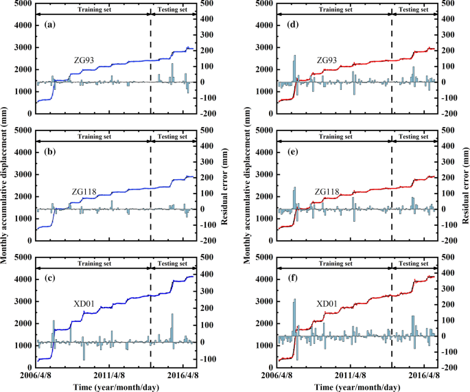

  

  Point prediction results based on the modified (a–c) and unmodified models (d–f)

• 4. Effect evaluation of interval prediction As shown in Table 7, the PICPs were all higher than the corresponding PINCs, demonstrating that the PIs of displacements constructed by the proposed model can completely encapsulate the measured displacement monitoring curves. As shown in Fig. 11a–c, the model flexibly quantified the uncertainty impaction of the dynamic variations of external factors on the landslide deformation through the variation of PI widths. For example, when the landslide deformed dramatically from May to August in 2007 and from June to July in 2015, the widths of the PIs increased significantly. These findings indicated that at these times, the uncertainty in the landslide deformation was extremely high, and the risk of landslide disaster was also high.

  Fig. 11

  

  Interval prediction results based on the modified (a–c) and unmodified models (d–f) under the PINC of 99.00%

4 Discussion

4.1 Influences of different clustering methods on prediction results

As shown in Fig. 3, the division of deformation states was the foundation of the whole interval forecasting framework. To reveal the influences of different clustering methods on the prediction results, the clustering results and the overall prediction results obtained by applying the CFSFDP-based method (i.e., the modified model) and the K-means-based modified model were compared. As shown in Tables 5 and 8, the SCs of the results obtained by using the K-means-based modified model were all below or equal to those results obtained by applying the CFSFDP-based modified model, illustrating that the CFSFDP algorithm had more advantages than the K-means algorithm in the clustering process of the landslide deformation states. Moreover, by further comparing Tables 7 and 9, it was easily determined that the effect of the deformation state division could directly affect the point prediction accuracy and the interval prediction quality. The above results showed that improving the division effect of the deformation state can increase the prediction effect of the proposed model.

Table 8 Evaluation of the clustering results obtained by using the K-means-based modified model

Table 9 Evaluation of the comprehensive prediction results obtained by using the K-means-based modified model

4.2 Influences of different unbalanced data processing methods on the prediction results

To explore the influences of different unbalanced data processing methods on the prediction results, we compared the deformation state identification and displacement prediction results obtained by applying the modified comprehensive method and other three data balancing methods. As shown in Table 10, regardless of which imbalanced data processing method was used to process the landslide monitoring data, the ensemble classifier could accurately identify the landslide deformation state of the training set. However, for the testing set, the identification accuracies of the deformation states obtained by using the other three methods were quite different from those obtained by using the modified model. Because the modified comprehensive method combined the advantages of the EGA and ADASYN methods, a suitable amount of mutation state data with more useful information was adaptively synthesized. Therefore, compared with the results obtained by using the other three methods, the specificities and G_means obtained by the modified method both reached the maximum levels.

Table 10 Evaluation and comparison of different unbalanced data processing methods on the performance of ensemble classifier

Sections 2.2.2 and 2.2.4 indicate that deformation state identification is another critical part of the construction of an interval forecasting model framework. The accuracy of the identification method can directly affect the performance of the hybrid model. Thus, as the critical link affecting the identification effect of the model on deformation states, the imbalanced data processing method can inevitably affect the prediction results. As shown in Tables 7 and 11, the differences between the landslide displacement point prediction and interval prediction results obtained by these four imbalanced methods were pronounced. The $R^{2}$ values of the point prediction results obtained by implanting the modified method were high and corresponded to low RMSEs. Meanwhile, the MPIWs and the CWCs of their PIs were the smallest. These results show that by using the modified method, the underfitting problem in the ensemble regressor caused by the confusion of different deformation state data was effectively solved to a certain extent. Thus, with the increase in the identification accuracy, the point prediction accuracy of the hybrid model was improved. Meanwhile, the PI width was effectively reduced under the same PINC.

Table 11 Evaluation and comparison of different unbalanced data processing methods on the point and interval prediction results

From the above results, we conclude that when constructing a displacement interval prediction model for step-like landslides, the improvement in the deformation state recognition effect is consistent with the improvement in the comprehensive performance of the proposed model. Therefore, how to properly manage the problem of the imbalance between the stable state and mutation state samples had become a significant point in the construction of the dynamic identification criteria of the deformation state. Compared with the traditional methods, the proposed comprehensive processing method can not only improve the accuracy of the ensemble classifier but also effectively increase the accuracy of the point prediction result and the quality of the PIs, thus highlighting the effectiveness and superiority of this method itself.

4.3 Performance comparison between the traditional interval prediction model and the improved interval prediction model

To verify the accuracy and superiority of the proposed modified model, the unmodified model without considering the dynamic switching of the deformation states was used as the comparison model. Tables 7 and 10 show that almost all the $R^{2}$ values of the modified model were higher than those of the unmodified model. Almost all the RMSEs of the modified model were lower than those of the unmodified model. Moreover, as shown in Fig. 10, although the predicted values of the mutation state samples obtained using the modified method still underestimated their actual values, the errors of the predicted values were decreased compared with the results obtained by the unmodified model. For instance, for monitoring site ZG118, when the Baishuihe landslide underwent severe deformation from the end of May to August 2007 and from June to July 2015, the underestimations of the predicted values decreased from 140.29 mm and 76.98 mm to 36.92 mm and 30.06 mm, respectively. However, although the hysteresis of the predicted values was improved, the differences between the predicted values and the actual values sometimes exceeded 100.00 mm. If these prediction results were directly applied to the early warning of actual step-like landslide disasters, these differences would not be acceptable without knowing the reliability of the prediction results.

In terms of the interval prediction results, the ensemble regression of the unmodified method was underfitting because the unmodified model was trained according to the mixed data without distinguishing the different deformation states of the data. As a result, under the same PINC, the MPIWs and CWCs of the PIs obtained using the unmodified model were significantly higher than those obtained by applying the modified model (Tables 7, 12). For the modified model, its ensemble regressors were separately constructed with data from different deformation states. Therefore, the prediction accuracies of the modified model were less affected by the mixing of the training data. The differences in the PI width under different deformation states were very apparent (Fig. 11). The PI widths under the mutation state were more significant than those under the stable state. Compared with the PIs obtained by applying the unmodified method, the PIs obtained by applying the modified method were more consistent with the deformation evolution characteristics of step-like landslides.

Table 12 Evaluation of comprehensive prediction results obtained by using the unmodified model

5 Conclusion

Under the coupling effect of reservoir water level fluctuation and durative heavy precipitation, the displacements of many reservoir colluvial landslides in the TGR area display obvious step-like behaviors. At present, the machine learning models used for landslide displacement prediction are mostly the point prediction models. This means that most of these models can accurately predict this kind of step-like displacement of landslides but are hard to express the reliability of their prediction results quantitatively. Thus, based on the idea of interval forecasting and the deformation state dynamic switching model of step-like landslides, a novel hybrid interval prediction model was proposed in this study.

The proposed hybrid interval prediction model consists of deformation state division, deformation state identification, prediction model establishment for the different deformation states, and dynamic prediction considering the dynamic switching of the deformation states. Taking the Baishuihe landslide as an example, the process of using this model to predict the landslide displacement and its PIs was introduced in detail. In the prediction performance comparison, two core issues related to improving the performance of the proposed model were also discussed in detail.

The results show that compared with the existing point prediction models, the proposed model can provide exact upper and lower limits of the PIs under certain nominal confidences to represent the reliability of the prediction results quantitatively. On the other hand, compared with the existing interval prediction model, the proposed model can not only improve the accuracy of the point prediction results but also promote the quality of the PIs. In addition, improvements in the deformation state division and the deformation state identification are found to have a positive correlation with the improvement in the comprehensive performance of the proposed model.

Overall, the proposed model performs well in terms of effectiveness, accuracy, and reliability and can provide more valid information for decision-makers. Thus, this model is of great significance for realizing accurate and reliable early warning systems of landslides whose deformation reflects the characteristics of a step-like evolution in the TGR area. Furthermore, from the perspective of landslide risk assessment, the proposed model is also worth promoting for use in predicting other types of landslides.

References

Breiman L (2001) Random forests. Mach Learn 45(1):5–32
Cai Z, Xu W, Meng Y, Shi C, Wang R (2016) Prediction of landslide displacement based on GA-LSSVM with multiple factors. Bull Eng Geol Environ 75(2):637–646
Cao Y, Yin K, Alexander DE, Zhou C (2016) Using an extreme learning machine to predict the displacement of step-like landslides in relation to controlling factors. Landslides 13(4):725–736
Du J, Yin K, Lacasse S (2013) Displacement prediction in colluvial landslides, Three Gorges reservoir, China. Landslides 10(2):203–218
Faculty of civil and construction, Three Gorges University (2013) Emergency management survey report of the Baishuihe Landslide, subsequent geological disaster prevention and control of Zigui County project in the Three Gorges Reservoir area. Three Gorges University, Yichang
Glade T, Anderson M, Crozier MJ (2005) Landslide hazard and risk: issues, concepts and approach. Landslide hazard and risk. Wiley, Chichester, pp 1–40
Gorsevski PV, Gessler PE, Jankowski P (2003) Integrating a fuzzy k-means classification and a Bayesian approach for spatial prediction of landslide hazard. J Geogr Syst 5(3):223–251
He H, Bai Y, Garcia EA, Li S (2008) ADASYN: adaptive synthetic sampling approach for imbalanced learning. In: 2008 IEEE international joint conference on neural networks (IEEE world congress on computational intelligence). IEEE, pp 1322–1328
He K, Wang S, Du W, Wang S (2010) Dynamic features and effects of rainfall on landslides in the Three Gorges Reservoir region, China: using the Xintan landslide and the large Huangya landslide as the examples. Environ Earth Sci 59(6):1267–1274
Huang GB, Zhou H, Ding X, Zhang R (2011) Extreme learning machine for regression and multiclass classification. IEEE Trans Syst Man Cybern Part B (Cybern) 42(2):513–529
Huang F, Huang J, Jiang S, Zhou C (2017) Landslide displacement prediction based on multivariate chaotic model and extreme learning machine. Eng Geol 218:173–186
Intrieri E, Carlà T, Gigli G (2019) Forecasting the time of failure of landslides at slope-scale: a literature review. Earth Sci Rev 193:333–349
Khosravi A, Nahavandi S, Creighton D, Atiya AF (2011) Comprehensive review of neural network-based prediction intervals and new advances. IEEE Trans Neural Netw 22(9):1341–1356
Li C, Tang H, Ge Y, Hu X, Wang L (2014) Application of back-propagation neural network on bank destruction forecasting for accumulative landslides in the three Gorges Reservoir Region, China. Stoch Environ Res Risk Assess 28(6):1465–1477
Lian C, Zeng Z, Yao W, Tang H (2013) Displacement prediction model of landslide based on a modified ensemble empirical mode decomposition and extreme learning machine. Nat Hazards 66(2):759–771
Lian C, Zeng Z, Yao W, Tang H (2014a) Ensemble of extreme learning machine for landslide displacement prediction based on time series analysis. Neural Comput Appl 24(1):99–107
Lian C, Zeng Z, Yao W, Tang H (2014b) Extreme learning machine for the displacement prediction of landslide under rainfall and reservoir level. Stoch Environ Res Risk Assess 28(8):1957–1972
Lian C, Chen CP, Zeng Z, Yao W, Tang H (2016) Prediction intervals for landslide displacement based on switched neural networks. IEEE Trans Reliab 65(3):1483–1495
Lian C, Zhu L, Zeng Z, Su Y, Yao W, Tang H (2018) Constructing prediction intervals for landslide displacement using bootstrapping random vector functional link networks selective ensemble with neural networks switched. Neurocomputing 291:1–10
Liao K, Wu Y, Miao F, Li L, Xue Y (2020) Using a kernel extreme learning machine with grey wolf optimization to predict the displacement of step-like landslide. Bull Eng Geol Environ 79(2):673–685
Ma J, Tang H, Liu X, Wen T, Zhang J, Tan Q, Fan Z (2018) Probabilistic forecasting of landslide displacement accounting for epistemic uncertainty: a case study in the Three Gorges Reservoir area, China. Landslides 15(6):1145–1153
Miao H, Wang G, Yin K, Kamai T, Li Y (2014) Mechanism of the slow-moving landslides in Jurassic red-strata in the Three Gorges Reservoir, China. Eng Geol 171:59–69
Miao F, Wu Y, Xie Y, Yu F, Peng L (2017) Research on progressive failure process of Baishuihe landslide based on Monte Carlo model. Stoch Environ Res Risk Assess 31(7):1683–1696
Miao F, Wu Y, Xie Y, Li Y (2018) Prediction of landslide displacement with step-like behavior based on multialgorithm optimization and a support vector regression model. Landslides 15(3):475–488
Mirjalili S, Mirjalili SM, Lewis A (2014) Grey wolf optimizer. Adv Eng Softw 69:46–61
Ren F, Wu X, Zhang K, Niu R (2015) Application of wavelet analysis and a particle swarm-optimized support vector machine to predict the displacement of the Shuping landslide in the Three Gorges, China. Environ Earth Sci 73(8):4791–4804
Rodriguez A, Laio A (2014) Clustering by fast search and find of density peaks. Science 344(6191):1492–1496
Tang H, Wasowski J, Juang CH (2019) Geohazards in the three Gorges Reservoir Area, China-Lessons learned from decades of research. Eng Geol 261:105267
Wang Y, Tang H, Wen T, Ma J (2019) A hybrid intelligent approach for constructing landslide displacement prediction intervals. Appl Soft Comput 81:105506
Wang Y, Huang J, Tang H (2020) Global sensitivity analysis of the hydraulic parameters of the reservoir colluvial landslides in the Three Gorges Reservoir area, China. Landslides 17(2):483–494
Wen T, Tang H, Wang Y, Lin C, Xiong C (2017) Landslide displacement prediction using the GA-LSSVM model and time series analysis: a case study of Three Gorges Reservoir, China. Nat Hazards Earth Syst Sci 17(12):2181
Wu Y, Chen C, He G, Zhang Q (2014) Landslide stability analysis based on random-fuzzy reliability: taking Liangshuijing landslide as a case. Stoch Environ Res Risk Assess 28(7):1723–1732
Xu Q, Tang M, Huang R (2015) Monitoring, early warning and emergency disposition for large-scale landslides. Science Press, Beijing, pp 22–27
Xue Y, Wu Y, Miao F, Li L, Liao K, Ou G (2020) Effect of spatially variable saturated hydraulic conductivity with non-stationary characteristics on the stability of reservoir landslides. Stoch Environ Res Risk Assess 34:311–329
Yang B, Yin K, Lacasse S, Liu Z (2019) Time series analysis and long short-term memory neural network to predict landslide displacement. Landslides 16(4):677–694
Yao W, Li C, Zuo Q, Zhan H, Criss RE (2019) Spatiotemporal deformation characteristics and inducing factors of Baijiabao landslide in Three Gorges Reservoir region, China. Geomorphology 343:34–47
Yi Q, Zhang M, Wen Kai XuX, Shang M (2017) Periodic analysis of deformation characteristics and influential factors of Baishuihe Landslide in three gorges reservoir area. J China Three Gorges Univ (Nat Sci) 39(1):38–42 (in Chinese)
Zhou C, Yin K, Cao Y, Ahmed B (2016) Application of time series analysis and PSO–SVM model in predicting the Bazimen landslide in the Three Gorges Reservoir, China. Eng Geol 204:108–120
Zhou P, Li Z, Snowling S, Baetz BW, Na D, Boyd G (2019) A random forest model for inflow prediction at wastewater treatment plants. Stoch Environ Res Risk Assess 33(10):1781–1792
Zhou C, Yin K, Cao Y, Intrieri E, Ahmed B, Catani F (2018) Displacement prediction of step-like landslide by applying a novel kernel extreme learning machine method. Landslides 15(11):2211–2225
Zhu X, Xu Q, Tang M, Li H, Liu F (2018) A hybrid machine learning and computing model for forecasting displacement of multifactor-induced landslides. Neural Comput Appl 30(12):3825–3835
Zou Z, Yang Y, Fan Z, Tang H, Zou M, Hu X, Meng Z, Xiong C, Ma J (2020) Suitability of data preprocessing methods for landslide displacement forecasting. Stoch Environ Res Risk Assess. https://doi.org/10.1007/s00477-020-01824-x
Acknowledgements
This research was supported by the National Natural Science Foundation of China (41977244) and the National Key R&D Program of China (2017YFC1501301). The authors thank the colleagues in our laboratory for their constructive comments and assistance. In addition, the authors would like to express their special thanks to Editors, two anonymous reviewers, and Dr. Yao Wenmin for their sincere assistance in improving this study. The dataset is provided by National Cryosphere Desert Data Center. (http://www.ncdc.ac.cn).
Author information
Authors and Affiliations
Corresponding author
Additional information
Publisher's Note
Springer Nature remains neutral with regard to jurisdictional claims in published maps and institutional affiliations.
Rights and permissions
About this article
Cite this article
Li, L., Wu, Y., Miao, F. et al. A hybrid interval displacement forecasting model for reservoir colluvial landslides with step-like deformation characteristics considering dynamic switching of deformation states. Stoch Environ Res Risk Assess 35, 1089–1112 (2021). https://doi.org/10.1007/s00477-020-01914-w
Accepted:
Published:
Issue Date:
DOI: https://doi.org/10.1007/s00477-020-01914-w