Gathering on rings under the Look–Compute–Move model

Abstract

A set of robots arbitrarily placed on different nodes of an anonymous ring have to meet at one common node and there remain. This problem is known in the literature as the gathering. Anonymous and oblivious robots operate in Look–Compute–Move cycles; in one cycle, a robot takes a snapshot of the current configuration (Look), decides whether to stay idle or to move to one of its neighbors (Compute), and in the latter case makes the computed move instantaneously (Move). Cycles are asynchronous among robots. Moreover, each robot is empowered by the so called multiplicity detection capability, that is, it is able to detect during its Look operation whether a node is empty, or occupied by one robot, or occupied by an undefined number of robots greater than one. The described problem has been extensively studied during the last years. However, the known solutions work only for specific initial configurations and leave some open cases. In this paper, we provide an algorithm which solves the general problem but for few marginal and specific cases, and is able to detect all the ungatherable configurations. It is worth noting that our new algorithm makes use of some previous techniques and unifies them with new strategies in order to deal with any initial configuration, even those left open by previous works.

1 Introduction

We study one of the most fundamental problems of self-organization of mobile entities, known in the literature as the gathering problem (see e.g., [9, 13, 18] and references therein). In particular, we consider oblivious robots initially located at different nodes of an anonymous ring that have to gather at a common node and there remain. Neither nodes nor links are labeled. Initially, each node of the ring is either occupied by one robot or empty. Robots operate in Look–Compute–Move cycles. In each cycle, a robot takes a snapshot of the current global configuration (Look), then, based on the perceived configuration, takes a decision to stay idle or to move to one of its adjacent nodes (Compute), and in the latter case it moves to this neighbor (Move), eventually. When a robot changes its position from a node to an adjacent one, we say that it performed a move. If $x$ robots make a move synchronously, it equals to perform $x$ moves. Indeed, Look–Compute–Move cycles are performed asynchronously for each robot. This means that the time between Look, Compute, and Move operations is finite but unbounded, and it is decided by the adversary for each robot. Hence, robots may move based on significantly outdated perceptions. We consider a minimalist variant of the Look–Compute–Move model which has very weak hypothesis. Neither nodes nor edges of the graph are labeled and no local memory is available on nodes. Robots are anonymous, uniform (i.e. they all execute the same algorithm), oblivious (memoryless) and have no common sense of orientation. We assume that moves are instantaneous, and hence any robot performing a Look operation sees all other robots on nodes and not on edges. Note that, in a discrete asynchronous environment this does not constitute a limitation to the model. In fact, an algorithm cannot take advantages from seeing robots on the edges as the adversary can decide to perform the Look operations only when the robots are on the nodes. On the other hand, if an algorithm takes advantage from the assumption that the robots always occupy nodes, the same algorithm can be applied by adding the rule that if a robot sees another robot on an edge, it just don’t move (i.e. it waits until all the robots occupy only nodes).

Robots are empowered by the so-called multiplicity detection capability [19]. That is, a robot is able to perceive whether a node of the network is empty, occupied by a single robot or by more than one (i.e., a multiplicity occurs), but not the exact number. Without multiplicity detection, the gathering has been shown to be impossible on rings [24].

1.1 Related work

The problem of gathering mobile entities on graphs [2, 14, 24] or open spaces [6, 13, 26] has been extensively studied in the last decades. When only two robots are involved, the problem is usually referred to as the rendezvous problem [1, 5, 7, 14, 27]. Under the Look–Compute–Move model, many problems have been addressed, like the graph exploration, the perpetual graph exploration [4, 12, 16, 17], and the perpetual graph searching [3, 12] while the rendezvous problem has been proved to be unsolvable on rings [24].

Concerning the gathering, different types of robot disposals on rings (configurations) have required different approaches. In particular, periodicity and symmetry arguments have been exploited. A configuration is called periodic if it is invariable under non-trivial (i.e., non-complete) rotation. A configuration is called symmetric if the ring has a geometrical axis of symmetry, that reflects single robots into single robots, multiplicities into multiplicities, and empty nodes into empty nodes. A symmetric configuration with an axis of symmetry has an edge–edge symmetry if the axis goes through two edges; it has a node–edge symmetry if the axis goes through one node and one edge; it has a node–node symmetry if the axis goes through two nodes; it has a robot-on-axis symmetry if there is at least one node on the axis of symmetry occupied by a robot. In [24], it is proved that the gathering is not solvable for periodic configurations, for those with edge–edge symmetry, and if the multiplicity detection capability is removed. Then all configurations with an odd number of robots, and all the asymmetric configurations with an even number of robots have been solved by different algorithms. In [23], the attention has been devoted to the symmetric cases with an even number of robots, and the problem was solved when the number of robots is greater than $18$. These results left open the gatherable symmetric cases of an even number of robots between $4$ and $18$. Most of the cases with $4$ robots have been solved in [25]. The cases left open in [25], referred to as the set $\mathtt {SP}4$, are symmetric configurations of type node–edge with $4$ robots and the odd interval cut by the axis bigger than the even one, with an interval being a maximal set of empty consecutive nodes. In general, configurations in $\mathtt {SP}4$ are ungatherable as outlined in [23] for configurations of $4$ robots on a five nodes ring. Actually, specific configurations in $\mathtt {SP}4$ could be gatherable but requiring suitable strategies difficult to be generalized. The main difficulty faced when dealing with configurations in $\mathtt {SP}4$ comes from the fact that among the two intervals cut by the axis, the odd one is bigger than the even one. Intuitively, the middle node of the odd interval is the only possible candidate to finalize the gathering, and this has been also proved in [15]. Hence, when robots move towards such a node to make a multiplicity, it may happen that only one of the two symmetric robots allowed to move makes the movement. The subsequent configuration contains now two intervals of even size corresponding to those intervals originally cut by the axis of symmetry. Possibly, they can be of the same size and hence they may induce different symmetries with respect to the original one.

Finally, the case of $6$ robots with an initial axis of symmetry of type node–edge, or node–node has been solved in [9].

Besides the cases left open, a unified algorithm that handles all the above cases is also missing.

Other interesting gathering results on rings concern the case of the so called local weak multiplicity detection. That is, a robot is able to perceive the multiplicity only if it is part of it. On this respect, our assumption in the rest of the paper concerns the global weak multiplicity detection. Whereas, the strong version would provide the exact number of robots on a node.

Using the local weak assumption, not all the cases have been addressed so far. In [20], it has been proposed an algorithm for aperiodic and asymmetric configurations with the number of robots $k$ strictly smaller than $\left\lfloor \frac{n}{2}\right\rfloor$, with $n$ being the number of nodes composing the ring. In [21], the case where $k$ is odd and strictly smaller than $n-3$ has been solved. In [22], an algorithm for the case where $n$ is odd, $k$ is even, and $10 \le k \le n-5$ is provided. Recently, the case of asymmetric configurations has been fully characterized in [12]. The remaining cases are still open and a unified algorithm like the one we are proposing here for the global weak assumption is not known.

Without any multiplicity detection, in [8, 11] the grid and the tree topologies have been fully characterized.

1.2 Our results

From the literature, we know that the configurations which are periodic, have an edge–edge symmetry, or contain only 2 robots cannot achieve the gathering. We denote the set of such configurations as $\mathtt {NG}$ (Not-Gatherable). Moreover, let $\mathtt {I}$ be the set of any possible initial configuration (i.e those configurations without multiplicities).

In this paper, we present a new distributed algorithm that achieves the gathering for any initial configuration in $\mathtt {I}\setminus (\mathtt {NG}\cup \mathtt {SP}4)$ by using the multiplicity detection. We denote the set of such configurations as $\mathtt {A}$ (Admissible). Our algorithm introduces a new approach and for some special cases makes use of previous ones. In particular, existing algorithms are used as subroutines for solving the basic gatherable cases with 4 or 6 robots from [25] and [9], respectively. Also, we exploit the following property.

Property 1

[24] Let $C$ be a symmetric configuration with an odd number of robots, without multiplicities. Let $C'$ be the configuration resulting from $C$ by moving the unique robot on the axis to any of its adjacent nodes. Then $C'$ is either asymmetric or still symmetric but aperiodic. Moreover, by repeating this procedure a finite number of times, eventually the configuration becomes asymmetric (with possibly one multiplicity).

For all the other gatherable configurations but the possible ones in $\mathtt {SP}4$, we design a new approach that has been suitably unified with the mentioned subroutines. Our result answers to the posed conjectures concerning the gathering, hence closing all the cases left open, and providing a general approach that can be applied to all the initial configurations in $\mathtt {A}$. In particular, the case of symmetric and gatherable configurations with and even number of robots between $8$ and $18$ has been solved. Moreover, the algorithm that solves such case is also able to solve the known gatherable cases by introducing new techniques without colliding with the used subroutines. The main result of this paper can be stated as follows.

Theorem 1

There exists a distributed algorithm for gathering any configuration in $\mathtt {A}$. The algorithm also allows robots to recognize whether a configuration is in $\mathtt {NG}\cup \mathtt {SP}4$.

1.3 Structure of the paper

In the next section we formally define the model, give the notation used in the paper, prove some preliminary results and give an overview of our new algorithm. In Sect. 3, we formally describe our algorithm and prove its correctness. In Sect. 4 we conclude the paper and outline some possible future research directions. The “Appendix” provides graphical representations of the algorithm.

2 Definitions and preliminaries

We consider an $n$-nodes anonymous ring without orientation. Initially, $k$ nodes of the ring are occupied by $k$ robots. During a Look operation, a robot perceives the relative locations on the ring of multiplicities and single robots.

The global status of the system can be defined by the current disposal of the robots plus their status, that is, whether they are performing the Look, the Compute, or the Move operation or they are simply inactive.

If an algorithm allows at least two robots to move concurrently, then there might be a so called pending move. This occurs when, due to the asynchrony, one of the robots allowed to move performs its entire Look–Compute–Move cycle while one of the others does not perform the Move phase, i.e. its move is pending. Clearly, all the other robots performing their cycle are not aware whether there is a pending move, that is they cannot deduce the global status from their view.

The current disposal of the robots, referred to as a configuration, can be described in terms of the view of a robot $r$. An interval is a maximal set of empty consecutive nodes. We denote a configuration seen by $r$ as a tuple $Q(r)=(q_0,q_1,\ldots , q_j)$, $j\le k-1$, that represents the sequence of the intervals sizes read by $r$ traversing the ring in one direction, starting from $r$. Abusing the notation, for any $0\le i\le j$, we refer by $q_i$ not only to the size of the $i$th interval but also to the interval itself. Unless differently specified, we refer to $Q(r)$ as the lexicographical minimum view among the two possibilities. For instance, in the configuration of Fig. 1a, we have that $Q(x)=(1,2,1,3,1,2)$. A multiplicity is represented as $q_i=-1$ for some $0\le i\le j$, regardless the number of robots in the multiplicity. For instance, in the configuration of Fig. 1b, $Q(x)=(1,-1,0,1,0,-1,1,1,3,1)$. In case a configuration contains two consecutive multiplicities the view is represented as a sequence $(\ldots ,-1,0,-1,\ldots )$, where 0 represents the length of the interval between the two multiplicities. Given a generic configuration $C=(q_0,q_1,\ldots , q_j)$, let $\overline{C}=(q_0,q_j,q_{j-1},\ldots ,q_1)$, and let $C_i$ be the configuration obtained by reading $C$ starting from $q_i$, that is $C_i = (q_i,q_{(i+1)\mathrm{mod}\,j+1},\ldots , q_{(i+j)\mathrm{mod}\,j+1} )$. For instance, in the configuration of Fig. 1a, we have that if $C=Q(y) =(1,3,1,2,1,2)$, then $\overline{C} = (1,2,1,2,1,3)$ and $C_3 = (2,1,2,1,3,1)$. The above definitions imply:

Fig. 1

a The intervals between robots $y$, $z$ and $y'$, $z'$ are the supermins, while the supermin configuration view is $(1,2,1,2,1,3)$. b Black nodes represent multiplicities

Property 2

Given a configuration $C$,

• (i) there exists $0<i\le j$ such that $C=C_i$ iff $C$ is periodic;

• (ii) there exists $0\le i\le j$ such that $C=\overline{(C_i)}$ iff $C$ is symmetric;

• (iii) $C$ is aperiodic and symmetric iff there exists only one axis of symmetry.

The next definition represents the key feature for our algorithm since it has a twofold advantage. In fact, based on it, a robot can distinguish if the perceived configuration (during the Look phase) is gatherable and if it is one of the robots allowed to move (during the Compute phase).

Definition 1

Given a configuration $C=(q_0,q_1,\ldots , q_j)$ such that $q_i\ge 0$, for each $0\le i\le j$, the view defined as $C^{SM}=\min \{C_i,~ \overline{(C_i)},~|~ 0\le i\le j\}$ is called the supermin configuration view. An interval is called supermin if it belongs to the set $I_C=\{q_i ~|~ C_i=C^{SM} \text{ or } \overline{(C_i)}=C^{SM}, 0\le i\le j\}$.

For instance, in the configuration of Fig. 1a, $C^{SM} = Q(z) = (1,2,1,2,1,3)$. The next lemma, based on Definition 1, is exploited to detect possible symmetry or periodicity features of a configuration.

Lemma 1

Given a configuration $C=(q_0,q_1,\ldots , q_j)$ with $q_i\ge 0$, for each $0\le i\le j$:

• 1. $|I_C|=1$ if and only if $C$ is either asymmetric and aperiodic or it admits only one axis of symmetry passing through the supermin;

• 2. $|I_C|=2$ if and only if $C$ is either aperiodic and symmetric with the axis not passing through any supermin or it is periodic with period $\frac{n}{2}$;

• 3. $|I_C|>2$ if and only if $C$ is periodic, with period at most $\frac{n}{3}$.

Proof

1.$\Rightarrow$) If $|I_C|=1$ and $C$ is symmetric, then the statement holds as otherwise there exists another interval of the same size of supermin to which the supermin is reflected with respect to the axis. Moreover, the same should hold for every neighboring interval of the supermin and so forth. Since by hypothesis, the supermin is unique, there must exist at least two intervals of different sizes that are reflected by the supposed symmetry, and hence $C$ results asymmetric.

If $|I_C|=1$ and $C$ is asymmetric then it must be aperiodic, as otherwise there exists $0<i\le j$ such that $C=C_i$ and this implies more than one copy of the supermin.

1.$\Leftarrow$) If $C$ is asymmetric and aperiodic, then $C_i \ne \overline{(C_i)}$, $C_i\ne C_\ell$ and $C_i \ne \overline{(C_\ell )}$, for each $i$ and $\ell \ne i$ and hence a unique supermin must exist. If $C$ admits only one axis of symmetry traversing the supermin, then there exists a unique $0\le i\le j$ such that $C^{SM} = C_i = \overline{(C_i)}$ as otherwise Property 2 would imply the existence of other axes of symmetry, one for each supermin.

2.$\Rightarrow$) If $|I_C|=2$ and $C$ is asymmetric, then by Property 2, it is periodic and the period must be of $\frac{n}{2}$.

If $|I_C|=2$ and $C$ is aperiodic and symmetric, the axis of symmetry cannot pass through both the supermins. In fact, if it does, $C^{SM} = \overline{(C^{SM})} = (C^{SM})_{j/2} = \overline{((C^{SM})_{j/2})}$ that implies $(C^{SM})_{\lfloor j/4 \rfloor } = \overline{(C^{SM})}_{\lceil j/4 \rceil }$, i.e., there exists another axis of symmetry orthogonal to the first one that reflects the supermin into the other supermin. Hence, $C$ would be periodic.

If $|I_C|=2$ and $C$ is periodic and symmetric, then by Property 2 there exist an $i$ such that $C^{SM} = (C^{SM})_i$. If $i\ne j/2$, then there exists an $i'\ne i$ such that $C^{SM}_i = (C^{SM})_{i'}$ which implies that $|I_C|>2$, a contradiction. Therefore, the period is $\frac{n}{2}$.

2.$\Leftarrow$) If $C$ is aperiodic and symmetric with the unique axis not passing through any supermin, then each supermin must be reflected by the axis to another one. Moreover, there cannot be more than $2$ supermins, as by definition of supermin, these imply other axes of symmetry, i.e., by Property 2, $C$ is periodic. If $C$ is periodic with period $\frac{n}{2}$, then any supermin has an exact copy after $\frac{n}{2}$ nodes, and there cannot be other supermins, as otherwise the period would be smaller.

3.$\Rightarrow$) If $|I_C|>2$, then there are at least $3$ supermins, and hence $C$ has a period of at most $\frac{n}{3}$.

3.$\Leftarrow$) If $C$ has a period of at most $\frac{n}{3}$, then a supermin is repeated at least $3$ times in $C$. $\square$

2.1 A first look to the algorithm

The lemma above already provides useful information for a robot when it wakes up. In fact, during the Look operation, it can easily compute $|I_C|$. In order to recognize whether the current configuration belongs to $\mathtt {NG}\cup \mathtt {SP}4$, it is enough to check whether at least one of the following conditions holds: $k=2$; the configuration belongs to the set $\mathtt {SP}4$; the configuration admits an edge–edge axis of symmetry; the configuration is periodic. In the next section, we will show that all the other configurations are gatherable. From now on, we assume that the initial configurations do not belong to $\mathtt {NG}\cup \mathtt {SP}4$ and we will show that the algorithm does not generate configurations in $\mathtt {NG}\cup \mathtt {SP}4$.

The main strategy allows only movements that affect the supermin. In fact, if there is only one supermin (i.e. $|I_c|=1$), and the configuration allows its reduction, the subsequent configuration still has only one supermin (the same as before but reduced), or a multiplicity is created. In general, such a strategy, applied to asymmetric configurations or to symmetric ones with the axis passing through the supermin, leads to create a configuration with one multiplicity. The node with the multiplicity will constitute the place where the gathering will be easily finalized by collecting the closest robots to the multiplicity until no robots are left out.

For gatherable configurations with $|I_C|=2$, our algorithm requires more phases before creating the final multiplicity where the gathering terminates. In this case, there are two supermins that can be reduced. If both are reduced simultaneously, then the configuration is still symmetric and gatherable. Possibly, it contains two symmetric multiplicities. Actually, this is the status that we want to reach even when only one of the two supermins is reduced. In general, the algorithm tries to preserve the original symmetry or to create a gatherable symmetric configuration from an asymmetric one. It is worth to remark that in all symmetric configurations with an even number of robots, the algorithm allows the movement of two symmetric robots. Then it may happen that, after one move, the obtained configuration is either symmetric or it is asymmetric with a possible pending move. In fact, if only one robot among the two allowed to move performs its movement, it is possible that its symmetric one either has not yet started its Look phase, or it is taking more time. If there might be a pending move, then the algorithm forces it before any other decision. Note that, pending moves can only occur from symmetric configurations where two symmetric robots are allowed to move. Due to the asynchrony of the system, we cannot ensure that both symmetric robots perform their moves simultaneously. However, we will show that from asymmetric configurations with a possible pending move (i.e., at one allowed move from a possible symmetry) our algorithm provides the mean to recognize whether this may have occurred and allows to move only the robot that can (re-)establish the symmetry. In so doing, asymmetric configurations cannot produce pending moves as the algorithm allows the movement of only one robot. In fact, either we perform the possible pending move or we reduce the unique supermin by deterministically distinguishing among the two robots delimiting it, until one multiplicity is created. Finally, all the other robots will join the multiplicity one-by-one. In some cases, from asymmetric configurations at one “allowed” move from symmetry (i.e., with a possible pending move), robots must guess which move would have been realized from the symmetric configuration, and force it in order to avoid unexpected behaviors. By doing this correctly, the algorithm brings the configuration to have two symmetric multiplicities as above, eventually. From here, a new phase that collects all the other robots but few of them into the multiplicities starts. The robots that in this phase remain out of the multiplicities are used as compass for the other robots in order to keep trace of the direction where the final gathering will be accomplished. In practice, they serve as guards of the original axis of symmetry. In this phase, still symmetric configurations may become asymmetric at one move from symmetry, and each time this happens, the algorithm re-establishes the original symmetry. Once the desired symmetric configuration with two multiplicities and few single robots is achieved, a new phase starts and moves the two multiplicities to join each other. The node where the multiplicities join represents the final gathering location.

3 Gathering algorithm

The algorithm works in five phases that depend on the configuration perceived by the robots, see Fig. 2. First, it starts from a configuration without multiplicities and performs phase multiplicity–creation whose aim is to create one multiplicity, where all the robots will eventually gather, or a symmetric configuration with two multiplicities. In the former case, phase convergence is performed to gather all the robots into the multiplicity. In the latter case, phases collect and then multiplicity–convergence are performed in order to first collect all the robots but few into the two multiplicities and then to join the two multiplicities into a single one. After that, phase convergence is performed. Special cases of seven nodes and six robots are considered separately in phase seven-nodes. It will be clarified later that the loops appearing in Fig. 2 can be traversed only a finite number of times and the algorithm terminates in phase convergence.

Fig. 2

Phases interchanges

In the next subsections, we describe each phase and prove the correctness. We also show how robots interchange from one phase to another until the final gathering is achieved. For each phase, we distinguish a set of types of configuration and list them in the related subsection. In order to identify the correct phase, a robot computes the following parameters of a configuration $C=(q_0,q_1,\ldots , q_j)$.

• 1. Number of nodes in the ring, $n(C)$;

• 2. Number of multiplicities, $m(C)$;

• 3. Number of nodes occupied or number of robots in the case without multiplicities, $\omega (C)$;

• 4. Distance between single robots and multiplicities;

• 5. If $C$ is symmetric and, in the affirmative case, if the symmetry is allowed.

We provide the pseudo-code of the procedures performed by the robot in each phase. Such procedures take as input the configuration view and the type of configuration (denoted as CT). The way how a robot can identify the type of configuration by computing the above parameters will be described later (see Sect. 3.7). Section 3.8 proves the correctness of the entire algorithm.

3.1 Examples of execution

By referring to Fig. 3, we provide some more details on possible executions of our gathering algorithm.

Fig. 3

Two examples of possible executions of the gathering algorithm. Black nodes represent multiplicities

From the initial configuration of Fig. 3a, Property 1 is exploited instead of reducing the supermins, since the configuration is symmetric with a robot on the axis. This choice has been made for simplifying the algorithm in the successive phases. In the example, the robot on the axis chooses to move to its left side, obtaining the configuration of Fig. 3b. Such a configuration is asymmetric and it has only one supermin. Moreover, the robots can recognize that there are no pending moves. Therefore, the unique supermin is reduced until a multiplicity is created (phase multiplicity–creation). In the specific case, the configuration of Fig. 3c is obtained. From this point on, all the robots join the unique multiplicity one-by-one, until achieving the gathering as in Fig. 3d (phase convergence).

The initial configuration of Fig. 3e is asymmetric but it can be possibly obtained from a symmetric configuration with two supermins, by reducing one of them. We will show that this situation can be detected by the robots by computing the possible symmetric configuration. Therefore, differently from what shown in the previous example of Fig. 3b where the unique supermin is reduced, the possible original symmetry is (re-)established by performing the possible pending move. The obtained configuration is given in Fig. 3f, still remaining in phase multiplicity–creation. This kind of move will be performed until two symmetric multiplicities are created as in Fig. 3g. At this point, phase collect is performed, in order to gather the other robots (but few) into the two multiplicities. In Fig. 3h, only two robots have been left out from the multiplicities and they have served during phase collect to keep trace of the direction where to move. Afterward, in phase multiplicity–convergence, the two multiplicities are joined into a single multiplicity as shown in Fig. 3h. Then, phase convergence moves the two remaining single robots into the multiplicity, accomplishing the gathering task.

3.2 Phase multiplicity–creation

In this phase, the main idea is to reduce the supermin by enlarging the largest interval adjacent to it as follows.

Definition 2

Let $Q(r)=(q_0,q_1,\ldots , q_j)$ be a supermin configuration view, then robot $r$ performs reduction if its movement leads to configuration $(q_0-1,q_1,\ldots , q_j+1)$.

The pseudo-code of reduction is given in Fig. 4. The procedure checks whether the robot perceives the supermin configuration view by comparing the configuration $C$ perceived by the robot with $C^{SM}$. Note that, in asymmetric configurations, the robot that perceived $C^{SM}$ is the one among the two robots at the extremities of the supermin allowed to move. In fact, the robot on the other extremity would perceive configuration $\overline{C}$ and, by definition of $C^{SM}$, we have $C^{SM} = C < \overline{C}$, as the configuration is asymmetric. Then, the procedure moves the robot towards the supermin (see the move that leads from configuration in Fig. 3b to that in Fig. 3c). In symmetric configurations, the test at line 1 returns true for both robots adjacent to the unique supermin or for the two symmetric robots that perceive $C^{SM}$ in case that $|I_C|=2$.

Fig. 4

Procedure reduction

It is worth to note that, from a symmetric configuration, always two robots can perform the reduction. If only one of them does it, the obtained configuration will contain exactly one supermin (see e.g. Fig. 3e). However, the original axis of symmetry can be preserved (like in the example of Fig. 3e, f). In fact, if the perceived configuration contains only one supermin and it is not symmetric, the robots are able to understand whether there might be a pending move to re-establish the original symmetry or not. In doing so, the robots can distinguish between asymmetric configurations with a possible pending move from those where no pending moves are possible. In the first case, the original symmetry is re-established (even though the starting configuration was not symmetric as for configuration in Fig. 3e), while in the second case there is only one supermin which is reduced (as for configuration in Fig. 3b).

This constitutes one of the main results of the paper and it is obtained by exploiting the following lemma.

Lemma 2

Let $C\in \mathtt {A}$ and let $C'$ be the configuration obtained from $C$ after a reduction performed by only one robot. If $C$ is asymmetric then $C'$ is at least at two moves from a symmetric configuration; if $C$ is symmetric then $C'$ is at least at two moves from any other symmetric configuration with an axis of symmetry different from that of $C$.

Before formally prove the lemma we better provide some hints concerning the rationale behind it. Intuitively, if $C$ is asymmetric then there is only one supermin configuration view $C^{SM}= (q_0,q_1,\ldots ,q_j)$. Therefore, when reduction is performed, we obtain a configuration with view $C'=(q_0-1,q_1,\ldots ,q_j+1)$ and, since $q_0$ is the unique smallest interval in $C$, then $q_0-1$ is the smallest interval in $C'$ (i.e. $q_0-1< q_i$, for each $0\le i\le j$). From Lemma 1 follows that a possible axis of symmetry can only pass through such unique interval. However, the two intervals adjacent to it are necessarily different as $q_1\le q_j < q_j+1$. This implies that $C'$ is asymmetric. To show that $C'$ is at two moves from any symmetric configuration, we formally prove that the supermin view of $C'$ differs from any other views of $C'$ by at least two units (lexicographically). In fact, $C^{SM}$ differs from any other views of $C$ by at least one unit and in $C'$ the view has been reduced by one unit. If $C$ is symmetric, similar arguments can be applied as formally shown in the following proof.

Proof

By Lemma 1, two cases may arise: there exists only one supermin in $C$ or the configuration is symmetric and contains exactly two supermins.

In the former case, by Lemma 1, it is enough to show that $C'$ requires more than one move to create another supermin different from that of $C$. Let us consider the supermin configuration view $C^{SM} = (q_0,q_1,\ldots ,q_j)$. For the sake of simplicity, let us assume that, for each $i=1,2,\ldots ,j$, $(C^{SM})_i < \overline{((C^{SM})_i)}$. The case where, for some $i$, $(C^{SM})_i > \overline{((C^{SM})_i)}$ is similar. The case that $(C^{SM})_i = \overline{((C^{SM})_i)}$ cannot occur as, otherwise, there exists an axis of symmetry passing through $q_i$, but by Lemma 1, the possible axis of symmetry can only pass through $q_0$, as $|I_C|=1$. By definition of supermin, for each $(C^{SM})_i$, $i=1,2,\ldots ,j$, there exists $k_i \in \{0,1,\ldots ,j\}$ such that: $q_\ell = q_{(i+\ell )\mathrm{mod}\,j+1}$, for each $\ell < k_i$; and $q_{k_i}<q_{(i+k_i)\mathrm{mod}\,j+1}$. Note that $(i+k_i)\mathrm{mod}\,j+1 \ne 0$ as otherwise the hypothesis of minimality of $q_0$ is contradicted. Moreover, $k_i\ne j$ as otherwise $\sum _{\ell = 0}^j q_\ell = \sum _{\ell = 0}^{k_i} q_\ell < \sum _{\ell = 0}^{k_i} q_{(i+\ell )\mathrm{mod}\,j+1} = \sum _{\ell =0}^j q_{(i+\ell )\mathrm{mod}\,j+1}$, that is a contradiction. From $C'$, the supermin configuration view is $C'^{SM}=(q_0',q_1',\ldots ,q_j')= (q_0-1,q_1,\ldots ,q_j+1)$ and we have that, for each $i=1,2,\ldots ,j$, two cases may arise: if $k_i>0$, then $q_0' \!=\! q_0-1<q_i \!=\!q_i'$ and $q_{k_i}' = q_{k_i}<q_{(i+k_i)\mathrm{mod}\,j+1} =q'_{(i+k_i)\mathrm{mod}\,j+1}$; if $k_i=0$, then $q_0' =q_0-1 < q_i-1=q_i'-1$. In any case, $C'^{SM}$ differs from $(C'^{SM})_i$ by two units. It follows that $C'$ is at least two moves from any symmetric configuration with the axis different from that passing through the supermin. In fact, in order to obtain another axis of symmetry by performing only one move on $C'$, $(C'^{SM})_i$ has to differ from $C'^{SM}$ by at most one unit. This is enough to show the statement for the case of symmetric configurations with exactly one supermin. Regarding the asymmetric case, it remains to show that $C'$ is at least two moves from any symmetric configuration with the axis passing through the supermin. In an asymmetric configuration $C^{SM} = (q_0,q_1,\ldots ,q_j)$ there exists a $q_k$, $1\le k \le \frac{j}{2}$, such that $q_{\ell } = q_{(j+1 -\ell ) \mathrm{mod}\,j+1}$, for each $\ell < k$, and $q_{k} < q_{j+1-k}$. From $C'$, the supermin configuration view is $C'^{SM} = (q_0',q_1',\ldots ,q_j') = (q_0-1,q_1,\ldots ,q_j+1)$ and two cases may arise: if $k>1$, then $q_1'=q_1 =q_j < q_j+1 =q_j'$ and $q_{k}' = q_{k} < q_{j-1-k} = q_{j-1-k}'$; if $k=1$, then $q'_1=q_1 < q_j =q'_j-1$. It follows that $C'$ is at least two moves from any symmetric configuration with the axis passing through the supermin.

Regarding the case of symmetric configurations with exactly two supermins, we use similar arguments as above. Let us consider the supermin configuration view $C^{SM} = (q_0,q_1,\ldots ,q_j)$ and let us assume that $h$ is the index such that $C^{SM} = \overline{((C^{SM})_h)}$. By definition, for each $(C^{SM})_i$, $i\in \{1,2,\ldots ,j\}{\setminus } \{h\}$, there exists $k_i \in \{0,1,\ldots ,j\}$ such that: $q_\ell = q_{(i+\ell )\mathrm{mod}\,j+1}$, for each $\ell < k_i$, and $q_{k_i}<q_{(i+k_i)\mathrm{mod}\,j+1}$. As above we are assuming that $(C^{SM})_i < \overline{((C^{SM})_i)}$ and we can show that $k_i\ne j$, $k_i\ne (j+h)\mathrm{mod}\,j+1$, $(k_i+i)\mathrm{mod}\,j+1\ne 0$, and $(k_i+i)\mathrm{mod}\,j+1\ne h$. From $C'$, the supermin configuration view is $C'^{SM} = (q_0',q_1',\ldots ,q_j') = (q_0-1,q_1,\ldots ,q_j+1)$ and we have that, for each $i\in \{1,2,\ldots ,j\}{\setminus } \{h\}$ two cases may arise: if $k_i>0$, then $q_0' = q_0-1<q_i=q_i'$ and $q_{k_i}' = q_{k_i}< q_{(i+k_i)\mathrm{mod}\,j+1} =q_{(i+k_i)\mathrm{mod}\,j+1}'$; if $k_i=0$, then $q_0'=q_0-1 < q_i -1 =q'_i -1$. In any case, $C'^{SM}$ differs from $(C'^{SM})_i$ by two units. Similar arguments to the ones used for the asymmetric case can show that $C'$ is at least two moves from any symmetric configuration with the axis passing through the supermin. $\square$

It follows that a robot can deduce $C$ from $C'$ by enlarging the supermin of $C'$. This equals to reduce the largest adjacent interval (i.e., by performing the reduction backwards) hence deducing the possible original axis of symmetry and then performing the possible pending reduction (See e.g. the example of Fig. 3e).

Procedure symmetric in Fig. 5 exploits Property 2 to check whether a configuration $C$ is symmetric, periodic, or symmetric of type edge–edge. In detail, it first checks whether $C$ is symmetric (lines 3–4), then if it is periodic (lines 5–6) and finally if the symmetry is of type edge–edge (lines 7–8). The last case occurs when there exists an $i$ such that the axis of symmetry passes through an even $q_i$, and also $n$ is even.

Fig. 5

Algorithm to test if a configuration is in an allowed symmetry, that is, it is symmetric, aperiodic and the axis of symmetry does not pass through two edges

Procedure check_reduction in Fig. 6 checks whether an asymmetric configuration $C$ can be obtained from some allowed symmetric configuration $\hat{C}$ by performing reduction. Procedure pending_reduction in Fig. 7 performs the pending reduction.

Fig. 6

Algorithm to test if a configuration is at one move from reduction

Fig. 7

Procedure pending_reduction

At line 1, Procedure check_reduction looks for the index $k$ such that $q_k$ is the supermin, as it is the only candidate for being the interval that has been reduced by a possible reduction. Then, at lines 2–6, it computes the configuration $\hat{C}$ before the possible reduction. This is done by enlarging $q_k$ and reducing the largest interval among $q_{(k-1)\mathrm{mod}\,j+1}$ and $q_{(k+1)\mathrm{mod}\,j+1}$. If $q_{(k-1)\mathrm{mod}\,j+1}=q_{(k+1)\mathrm{mod}\,j+1}$ or $\textsc {symmetric}$ returns $\text{ false }$ on $\hat{C}$, then $C$ cannot be obtained by performing a reduction from an allowed symmetric configuration and the procedure returns ($\text{ false }$, $\emptyset$) (see lines 8 and 11). If $\textsc {symmetric}$ returns $\text{ true }$ on $\hat{C}$ (line 9), then $C$ can be obtained by performing reduction on $\hat{C}$ and hence the procedure returns ($\text{ true }$, $\hat{C}$) at line 10.

Procedure pending_reduction uses check_reduction to check whether $C$ can be obtained by performing reduction on a configuration $\hat{C}$ (lines 1 and 2). At line 2 the procedure checks whether the robot is at the extremity of one of the two supermins of $\hat{C}$ ($\min \{\hat{C}, \overline{(\hat{C}_j)}\} = \hat{C}^{SM}$) and if it has not yet performed reduction ($\min \{C ,\overline{(C_j)}\}\ne C^{SM}$). In the affirmative case, the robot has to move towards the supermin (line 3).

In general, it is not always possible to perform reduction as it may cause infinite computations. For instance, this can occur when there exists only one supermin of size 0 and the configuration is symmetric. In fact, by Lemma 1 the axis of symmetry passes through the edge between the two robots $r$ and $r'$ delimiting the supermin. Therefore, applying $\textsc {reduction}$ may consist in moving synchronously $r$ and $r'$ in opposite directions hence swapping their positions infinitely many times. Another case where it is not clear whether $\textsc {reduction}$ can be applied occurs in symmetric configurations with two supermins of size zero divided by one interval of even size. These two cases will be managed separately by means of two alternative moves. However, we will show that a robot is always able to understand that there might be a pending move also for the other moves allowed by our algorithm from symmetric configurations.

One of the alternative moves is based on the following definition.

Definition 3

Given a configuration $C=(q_0,q_1,\ldots , q_j)$, the view defined as $C^{ASM}=\min \{C_i,~ \overline{(C_i)}| C_i\ne \overline{(C_i)} \text{ and } C_i\ne C^{SM} \text{ and } \overline{(C_i)}\ne C^{SM},~0\le i\le j\}$ is called the alternative supermin configuration view, and its first interval is called alternative supermin.

When it is not possible to perform reduction, we either reduce the alternative supermin or we perform the xn move that is defined in the following.

Definition 4

Let $C$ be a configuration where $n(C)$ is odd, there are more than six robots, and there are no multiplicities:

• If $C$ is symmetric with only one supermin of size zero or with two supermins of size zero divided by one interval of even size, xn corresponds to moving towards the axis the two symmetric robots closest to the axis of symmetry that are divided by an odd interval;¹

• If $C$ is asymmetric and it has been possibly obtained by applying xn from a symmetric configuration $C'$ (that is, from $C'$ only one of the two robots on the above case has moved), then xn on $C$ corresponds to moving the second closest robot towards the axis of $C'$.

Each time a robot wakes up, it needs to find out which kind of configuration it is perceiving, and, if it is allowed to move, it needs to compute the right move to be performed. We need to distinguish among several types of configurations, requiring different strategies and moves. In this phase, as there are no multiplicities, a robot must distinguish among the following configurations:

• W1 Symmetric configurations with an odd number of robots;

• W2 Configurations with four robots;

• W3 Configurations with six robots;

• W4 Symmetric configurations with an even number of robots greater than six, only one supermin of size zero or with two supermins of size zero divided by one interval of even size (possibly of size zero) with no other intervals of size zero;

• W5 Symmetric configurations with an even number of robots greater than six, only one supermin of size zero or with two supermins of size zero divided by one interval of even size (possibly of size zero), and other intervals of size zero;

• W6 Asymmetric configurations with an even number of robots greater than six and:

  • (a) only one interval of size zero, and it is in between two intervals of equal size;

  • (b) only two intervals of size zero, with only one in between two intervals of equal size;

  • (c) only two intervals of size zero, with one even interval in between;

  • (d) only three intervals of size zero, with only two of them separated by an even interval;

  • (e) only three consecutive intervals of size zero;

  • (f) only four intervals of size zero, with only three of them consecutive;

• W7 Remaining configurations in $\mathtt {A}$.

For each configuration type, our algorithm checks whether the robot perceiving the configuration $C$ is allowed to move and eventually, performs the move. The moves that the robots can perform according to the perceived configurations are implemented by Procedure multiplicity–creation given in Fig. 9. Such moves induce the state diagram of Fig. 8 as long as they do not create multiplicities. In the following we describe the moves in detail assuming that a robot $r$ perceives a configuration $C=Q(r)=(q_0,q_1,\ldots ,q_j)$.

Fig. 8

Phase multiplicity–creation

Fig. 9

Procedure multiplicity–creation

From configurations in W1 (see lines 1–2), only the robot on the axis can move in one of the two directions, arbitrarily (see e.g. the example in Fig. 3a, b). Note that the robot on the axis is the unique robot that perceives a view $C$ such that $C=\overline{(C_j)}$. After this move either the configuration contains one multiplicity or it belongs to W1 or W7. With this respect, a graphical description of the possible transitions from W1 to the reachable configuration type can be found in “Appendix 1”. Configurations in W7 will be described later in this section and the configurations with multiplicities will be described within the other phases. Regarding configurations in W1, from Property 1, we know that the number of times that the obtained configuration remains in W1 after this move is bounded.

When the configuration is in W2 or in W3 (see lines 4–8), a modified version of algorithms in [25] and [9] are performed, respectively. In particular, both the algorithms are able to manage symmetric configurations and to check whether in an asymmetric configuration there is a possible pending move. If the configuration is not symmetric and there are no pending moves, then reduction is performed. The resulting configuration is still in W2 or in W3 or at least one multiplicity is created. Similarly to the case of W1, a graphical description of the possible transitions from W3 to the reachable configuration type can be found in “Appendix 1”.² From the correctness of algorithms in [25] and [9] and from the fact that performing reduction results in reducing the supermin, it follows that eventually at least one multiplicity is created. In the rest of the paper the two procedures in [25] and [9] are denoted as gather-four-nodes and gather-six-nodes, respectively. We assume that they return $\text{ true }$ if the configuration is not symmetric and there are no pending moves, and apply the corresponding algorithms otherwise.

When the configuration is in W7 (see lines 31–34) and it is symmetric, then the algorithm performs reduction on two symmetric robots that lead to another symmetric configuration in W7 (a limited number of times as above), or to a configuration with at least one multiplicity, or to an asymmetric configuration with a pending move. In this latter case, by Lemma 2 the algorithm recognizes that the configuration is at one “allowed” move from symmetry and performs the pending move (even though it was not pending, indeed). When the configuration is asymmetric without any possible pending move, again reduction is performed. By performing the described movements, at least one multiplicity is created.

Configurations in W4–W6 correspond to the cases where reduction is not allowed to be performed. In fact, if the configuration is symmetric and there is only one supermin of size zero, then reduction may result in swapping the robots at the extremities of the supermin, hence obtaining infinitely many times the same configuration. Similarly, if the configuration is symmetric and there are two symmetric supermins of size zero divided by one interval of even size, then reduction would produce two multiplicities divided by the interval of even size and we won’t be able to join such multiplicities afterwards.

From W4 (see lines 10–13), the algorithm performs xn, hence leading to configurations in W4, W6 or to configurations with one multiplicity on the axis. Note that, in these configurations, the axis always crosses the middle node of the interval delimited by the robots that perform xn. Therefore, if the configuration is again in $W4$, such robots keep on moving in the same direction and will eventually gather at the node crossed by the axis. Move xn is implemented by finding out the odd interval crossed by the axis of symmetry. The two robots at the extremities of such interval are the only ones that read a configuration $C$ such that either $C = \overline{C}$ with $q_0$ odd, or $C_j =\overline{(C_j)}$ with $q_j$ odd, depending on the orientation of the view.

From W5 (see lines 14–15), the algorithm performs reduction with respect to the alternative supermin instead of the supermin, according to Definition 3. Note that, as in this case the alternative supermin has size zero, we obtain at least one multiplicity.

The asymmetric configurations in W6 (see lines 17–29) are either asymmetric starting configurations or are obtained from the symmetric configurations in W4 after performing xn. In these cases, the algorithm checks whether the configuration is obtained after an xn move. This is realized by moving backward the robot closest to the other pole of the axis of symmetry that is assumed to pass through: The supermin in case (a); The only interval of size zero adjacent to two intervals of equal size in case (b); The even intervals mentioned in cases (c) and (d); the only interval of size zero in between other two intervals of size 0 in cases (e) and (f). If a backwards xn produces a symmetric configuration, then the symmetric xn is performed, otherwise, reduction is performed. In the former case, the configuration is either in $W4$ or it has one multiplicity on the axis, in the latter case, reduction creates a multiplicity.

Lemma 2, shows that performing $\textsc {reduction}$ on only one robot of a configuration $C$ does not create a symmetric configuration. Moreover, if $C'$ is the configuration obtained, then $C'$ cannot be obtained by applying any other move on a different symmetric configuration. The same holds if $C$ belongs to $W5$ where we apply reduction on the alternative supermin. In fact, performing such a move on only one robot creates a configuration with exactly one multiplicity which adjacent intervals differ by at least one unit. The next two lemmas show that this also holds for $\textsc {xn}$. In detail, the first lemma shows that a configuration $C$ in $W6$ can be obtained only if $C$ is in $W4$ or it is asymmetric, and the second one shows that there is only one configuration in $W4$ that generates $C$ by performing $\textsc {xn}$ on only one robot.

Lemma 3

Let $C$ be a symmetric configuration in $W7$ and let $C'$ be the configuration obtained from $C$ after a reduction move performed by only one robot. Then, $C'$ does not belong to $W6$.

Proof

If $C'$ contains multiplicities, then it does not belong to $W6$. Therefore, let us assume that $C'$ does not contain multiplicities.

Any configuration with more than one interval of size zero cannot be obtained after a reduction move performed by only one robot. In fact, a standard move would reduce at least one of the existing intervals of size zero, hence creating a multiplicity. Therefore, $C'$ cannot belong to cases (b)–(f) of $W6$.

If $C'$ belongs to case (a) of $W6$, then, the supermin is the only interval of size zero. However, such a configuration cannot be obtained by a reduction move as the two intervals adjacent to the supermin have equal size. $\square$

Lemma 4

Let $C$ be a configuration in $W4$ and let $C'$ be the configuration obtained from $C$ after an xn move performed by only one robot. Then $C'$ is asymmetric and it cannot be obtained after an xn move performed by only one robot from a configuration $C''\ne C$ in $W4$.

Proof

If $C$ belongs to $W4$, then it has either a unique supermin or two symmetric supermins given by the intervals of size zero. After performing xn by only one robot, the new configuration $C'$ can have: (i) one supermin corresponding to one interval of size zero of $C$, (ii) one supermin corresponding to the interval reduced by the performed move, or (iii) two supermins corresponding to the only interval of size zero of $C$ and to the interval reduced by the performed move, (iv) two supermins corresponding to one of the two intervals of size zero of $C$ and to the interval reduced by the performed move.

In case (i), by Lemma 1, if $C'$ is symmetric then the axis must cross the supermin. However, the two opposite views from such a supermin must be different as otherwise one of them corresponds to a view in $C$ which is smaller than the supermin configuration view $C^{SM}$, a contradiction.

In case (ii), the interval reduced by the performed move must be of size zero in $C'$. Hence, like in case (i), the axis must cross the unique supermin. However, the two intervals adjacent to such supermin are different as only one of them has been modified by the performed move.

In case (iii), the two intervals adjacent to the supermin of $C'$ corresponding to the only interval of size zero of $C$ must have the same size since the axis of $C$ crosses the interval of size zero and there are more than four robots. However, the two intervals adjacent to the one reduced by the performed move are different as only one of them has been modified, a contradiction.

In case (iv), the axis must cross the only interval of size zero which is not a supermin and therefore $C$ must contain exactly six robots, a contradiction.

To show that $C'$ cannot be obtained by performing xn by only one robot from a configuration $C''\ne C$ in $W4$, note that $C'$ belongs to $W6$. We hence analyze each of the cases (a)–(f) of $W6$. As there are more than six robots, $\textsc {xn}$ does not enlarge the intervals of size zero. It follows that $C''$ has at most the same number of intervals of size zero of $C'$.

In case (a), the only possible axis of symmetry of $C''$ must pass through the only interval of size zero. It follows that the xn performed by only one robot from $C''$ leads to reduce one of the two adjacent intervals to that on the axis of symmetry, antipodal to the interval of size zero. This is exactly what happens from $C$, and hence $C''$ cannot be different from $C$.

Similar arguments apply in other cases but the possible axis passes through: the unique interval of size zero between two intervals of equal size in case (b); the even interval between the two intervals of size zero in cases (c) and (d); the middle interval of size zero of the three consecutive ones in cases (e) and (f). $\square$

The next lemma states that multiplicity–creation eventually terminates with at least one multiplicity and hence one of the other phases starts.

Lemma 5

Phase multiplicity–creation terminates with either one or two symmetric multiplicities after a finite number of moves.

Proof

From the description provided before this lemma, it follows that the graph in Fig. 8 models the execution of phase multiplicity–creation. We now show that all the cycles are traversed a finite number of times. This implies that eventually either one or two symmetric multiplicities are created.

From Property 1, and results in [25], and [9] follows that the self-loops in W1, W2, and W3, respectively, are traversed a finite number of times.

The self-loop in W7 is traversed by performing reduction or pending_reduction. Each time such moves are performed, the supermin decreases until, after a finite number of moves, it either creates a multiplicity or leads to configurations in W4 or W6. The number of moves is at most two times the size of the initial supermin for symmetric configurations with the axis not passing through the supermin and it is the size of the initial supermin otherwise.

The self-loop in W4 and the cycle between W4 and W6 are traversed by performing xn. Each time this happens, the interval between the two symmetric robots closest to the axis of symmetry (excluding those adjacent to the supermin) is reduced until creating a multiplicity on the axis. The number of moves performed equals the initial size of such an interval. $\square$

If multiplicity–creation leads to a configuration with two symmetric multiplicities or at one move from a symmetric configuration with two multiplicities, then phases collect or multiplicity–convergence start. If it leads to a configuration with only one multiplicity which is not at one move from a symmetric configuration with two multiplicities, then phase convergence starts. Special cases on a seven nodes ring are addressed by phase seven-nodes.

3.3 Phase collect

In this phase, all the robots but four gather to the two symmetric multiplicities created in the previous phase. The rationale behind invoking this phase before joining the two multiplicities resides in making easy to the robots to recognize in which phase they are. In fact, anticipating the merging of the two multiplicities may lead to configurations with new axes of symmetry or at one step from other axes of symmetry with respect to the original one.

This phase can start only if the initial configuration is symmetric or at one step from specific symmetric configurations.

Before proceeding with the description of this phase, we need to distinguish among the two poles of an axis of symmetry in the case that there are two, three or four multiplicities. The cases of three and four multiplicities are handled in the successive phases. We call one of the poles north according to the following definition which is needed also in the successive phases.

Definition 5

In a symmetric configuration not in $\mathtt {NG}$ with two, three or four multiplicities, if the axis is of type node–edge, node–node, or robot–robot, then we call one node $\mathtt{north}$ as follows:

• node–edge axis case: the north is the middle node of the odd interval crossed by the axis;

• node–node axis case: let us consider the two sub-rings which are crossed by the axis and between two symmetric multiplicities. The north is the middle node of the smallest sub-ring, if the two sub-rings have different sizes. If the two sub-rings have the same size, then the north is the middle node of the interval crossed by the axis from which by reading all the configuration, one obtains the lexicographically largest string;

• robot–robot axis case: as for the previous case, let us consider the two sub-rings which are crossed by the axis and between two symmetric multiplicities. The north is the middle node of the smallest sub-ring, if the two sub-rings have different sizes. If the two sub-rings have the same size, then the north is the node occupied by the robot crossed by the axis from which by reading all the configuration, one obtains the lexicographically smallest string.

The other node or edge cut by the axis is called south.

In the cases with a robot-node or robot-edge symmetry (i.e. when the number of robots is odd) the algorithm does not generate configurations with more than one multiplicity. Therefore, in such cases, the definitions of north and south are not needed.

We assume that in symmetric configurations with multiplicities, a robot reads a configuration starting from the northern interval between the two adjacent ones. For instance, robots $x$ and $z$ of Fig. 1b, read $(1,-1,0,1,0,-1,1,1,3,1)$ and $(1,0,-1,1,1,3,1,1,-1,0)$, respectively. We also assume that if the robot belongs to a multiplicity the first interval $q_0$ is equal to $-1$. For instance, robots $y$ in Fig. 1b, read $(-1,0,1,0,-1,1,1,3,1,1)$.

In asymmetric configurations with one multiplicity, the proper reading of a robot is defined as follows. Let us consider the configuration read by a robot in an arbitrary order $C=(q_0,q_1,\ldots ,q_i,\ldots ,q_j)$, where $q_i=-1$. The robot first verifies whether there is another symmetric multiplicity to be created by checking whether the configuration $C'$ defined as $C'=(q_0,q_1,\ldots ,q_{i-1}-1,0,\ldots ,q_j)$ if $q_{i-1}>q_{i+1}$ or $C'=(q_0,q_1,\ldots ,0,q_{i+1}-1,\ldots ,q_j)$ if $q_{i-1}<q_{i+1}$ is symmetric. In the affirmative case, the robot chooses the proper reading between $C$ and $\overline{(C_j)}$ according to the minimal one between $C'$ and $\overline{(C'_j)}$ (see Fig. 10). Otherwise, and in the case that $q_{i-1}=q_{i+1}$, it chooses the one towards the multiplicity, that is $C$ if $\sum _{\ell =0}^{i-1} q_\ell \le \sum _{\ell =i+1}^j q_\ell$ and $\overline{(C_j)}$ otherwise (see Fig. 11).

Fig. 10

Let us assume that robot $x$ in a reads the configuration $C=(4,-1,2,1,2,0,3,1)$, where $q_i=-1$ for $i=1$. Then, it computes $C'=(3,0,2,1,2,0,3,1)$ represented in b. Since $C'$ is symmetric and $\overline{(C'_j)} <C'$, then $x$ sets as proper reading $\overline{(C_j)}=(1,2,0,2,1,2,-1,4)$

Fig. 11

Let us assume that robot $x$ in a reads the configuration $C=(4,-1,2,1,2,1,2,1)$, where $q_i=-1$ for $i=1$. Then, it computes $C'=(3,0,2,1,2,1,2,1)$ represented in b. Since $C'$ is asymmetric, then $x$ computes $\sum _{\ell =0}^{i-1} q_\ell = 4$ and $\sum _{\ell =i+1}^j q_\ell = 9$ and chooses $C$ as proper reading because $\sum _{\ell =0}^{i-1} q_\ell \le \sum _{\ell =i+1}^j q_\ell$

In asymmetric configurations with two multiplicities, in order to provide a robot with a proper reading, we need to recognize the north of a symmetric configuration from which the current configuration has been potentially obtained. In doing so, a robot will read the configuration starting from the northern interval among its adjacent ones. To this aim, the robot looks for an interval or a robot which is at the same distance from the two multiplicities. If there exists an interval of even size at the same distance from the two multiplicities, then the middle edge of such interval is identified as south and the node at distance $\lfloor \frac{n}{2} \rfloor$ from both the extremities of the south is identified as the north (see Fig. 12a). In any other case, we compare the sizes of the two sub-rings between the two multiplicities. If they are different, we consider the configuration obtained by removing all the single robots adjacent to the multiplicities. Then, the middle robot, or the middle node of the middle interval of the smallest sub-ring is identified as the north (see Fig. 12b). If they are equal, the algorithm ensures that there always exists an odd size interval or a robot at the same distance from the two multiplicities. Therefore, we lexicographically compare the configurations read by such interval (robot, resp.) with that read from the node at distance $\frac{n}{2}$ from the middle of this interval (from the robot, resp.) and consider the largest (smallest, resp.) as the north (south, resp.) and the other as south (north, resp.). See Fig. 12c for an example.

Fig. 12

Identifying north and south in asymmetric configurations with two multiplicities. a Since the interval between $x$ and $y$ is even and the distance between $m_1$ and $x$ is equal to that between $m_2$ and $y$, then the middle edge of the interval between $x$ and $y$ is identified as the south and the node $z$ is identified as north. b Since the sub-ring on the bottom of the two multiplicities is smaller that the one on top of them, then node $x$ (in the middle of the smallest sub-ring) is identified as north. c The two sub-rings on the top and bottom of the two multiplicities have the same size. Therefore, we compare the readings from nodes $y$ and $x$ which are $C_y=(1,2,-1,4,4,-1,1,2)$ and $C_x=(4,-1,1,2,1,2,-1,4)$, respectively. As $C_y<C_x$, then we choose $y$ as north and $x$ as south

In order to keep trace of the possible axis of symmetry that determines the final gathering node, we also introduce the concept of guards, identified by two single robots placed on specific nodes of the configurations handled in this phase. The guards are also exploited by robots to understand when phase collect (Fig. 13) has terminated.

Definition 6

Given a configuration with two multiplicities and at most six nodes occupied, two single robots are called guards if:

• they occupy the north and the south;

• they occupy the extremities of the interval containing the south.

Fig. 13

Phase collect

We remind that by construction, when the configuration contains two multiplicities, the north and the south poles are always well defined since the configuration is either symmetric or at one allowed move from symmetry. Hence, on such configurations with at most six nodes occupied the guards can be always detected. The limit of six nodes occupied has been set because it determines the moment when the robots exit from phase collect and enter phase multiplicity–convergence, and they never come back.

Fig. 14

Procedure collect

Phase collect is performed if one of the next configurations occurs:

• Coll-a-1 Asymmetric configurations with more than six nodes occupied, one multiplicity at more than one move from the symmetry passing through the multiplicity and at one move from the symmetry existing before performing reduction or reducing the alternative supermin;

• Coll-s-2 Symmetric configurations with two multiplicities and

  • (a) more than six nodes occupied;

  • (b) six nodes occupied and more than one single robot at distance greater than zero from any multiplicity on the northern side;

  • (c) six nodes occupied and more than two single robots at distance greater than zero from any multiplicity on the southern side;

• Coll-a-2 Asymmetric configurations with two multiplicities and

  • (a) more than six nodes occupied;

  • (b) six nodes occupied and at least one single robot which is not a guard at distance greater than zero from any multiplicity.

The pseudo-code of procedure collect is given in Fig. 14.

When the configuration is in Coll-a-1, the algorithm (lines 1–10) first checks whether the current configuration is at one move from the symmetric configuration existing before performing reduction or reducing the alternative supermin. If this condition is verified, it moves the robot that re-establishes the previous axis of symmetry, leading to a symmetric configuration which contains two multiplicities. Note that, the original configuration was at more than one move from the symmetry passing through the multiplicity. After this move, a configuration in Coll-s-2 is obtained. Then, the algorithm generates only configurations in Coll-s-2 or in Coll-a-2.

When the configuration is in Coll-s-2, we need to distinguish among the types of symmetry.

In node–node and node–edge symmetries (lines 12–16), we consider the two symmetric robots which are the closest ones to the multiplicities among those in the nodes between the multiplicities and the north. The algorithm moves these two robots symmetrically (generating again configurations in Coll-s-2 or in Coll-a-2 if the symmetric robots move synchronously or not, respectively) until they join the two multiplicities. This operation is iteratively performed by all the robots between the multiplicities and the north. The last two robots are allowed to join the multiplicities only if there are more than six nodes occupied. Otherwise, these two robots are moved until they become adjacent to the multiplicities. Then, the robots between the multiplicities and the south (but the guards), perform the same operation, starting by the two symmetric robots closest to the multiplicities.

In robot–robot symmetric configurations (lines 17–21), the behavior is similar but it is realized by first collecting the robots on the south and then those on the north, but for the guards.

In both cases, the algorithm eventually leads to a symmetric configuration with six nodes occupied by two multiplicities, two guards and two robots adjacent to the multiplicities. The next lemma shows that this phase eventually terminates in the described symmetric configuration.

Lemma 6

Phase collect terminates after a finite number of moves by reaching a symmetric configuration with six nodes occupied by two multiplicities, two guards and two single robots adjacent to the multiplicities.

Proof

From the above description, it follows that the graph in Fig. 13 models the execution of phase collect. We now show that all the cycles are traversed a finite number of times until one of the configurations in the statement is created.

There are only two cycles in the graph: the self-loop in Coll-s-2 and the bidirectional edge between Coll-s-2 and Coll-a-2. Each time that one of these two cycles is traversed, either the distance between a multiplicity and a robot or the number of single robots is decreased until six nodes are occupied by two multiplicities, two guards and two robots adjacent to the multiplicities. In fact, if at least one of the single robots which is not a guard is at distance greater than zero from any multiplicity, then the algorithm makes move it (and possibly its symmetric one) until this situation does not occur anymore, hence reducing the distance between single robots and multiplicities. $\square$

3.4 Phase multiplicity–convergence

This phase starts from a configuration of the type given in Lemma 6 and it aims to move the two multiplicities and the two single robots which are not the guards to the north. In so doing, all the robots but one, two, three or four, are gathered in the north node. The non gathered robots are the guards that might be one or two on the southern side, and those not yet entered the final multiplicity but adjacent to it (and these also might be one or two).

Phase multiplicity–convergence is performed if one of the next configurations occurs:

• Mc-s-x Symmetric configurations with

  • (a) two multiplicities with more than seven nodes and exactly four nodes occupied

  • (b) two multiplicities, two guards and two single robots adjacent to the multiplicities (six nodes occupied overall);

  • (c) three multiplicities or two multiplicities and exactly five nodes occupied;

  • (d) four multiplicities;

• Mc-a-x Asymmetric configurations with

  • (a) two multiplicities, more than seven nodes and less than six nodes occupied;

  • (b) two multiplicities, six nodes occupied and no single robots but the guards at distance greater than zero from any multiplicity;

  • (c) three multiplicities;

• Mc-a-1 Asymmetric configurations with more than seven nodes, five nodes occupied, one multiplicity at more than one move from the symmetry passing through the multiplicity and at one move from a symmetry allowed by algorithm in [9].

The pseudo-code of Procedure multiplicity–convergence is given in Fig. 15.

Fig. 15

Procedure multiplicity–convergence

From Mc-s-x, if there are two multiplicities, the algorithm moves them towards north if exactly four nodes are occupied (line 2), or if exactly six nodes are occupied with one single robot adjacent to the northern side of each multiplicity (second condition of line 11). If exactly six nodes are occupied with one single robot adjacent to the southern side of each multiplicity (first condition of line 11), the algorithm moves towards north the two symmetric robots adjacent to the multiplicities, making such robots joining the multiplicities. These operations lead to configurations in Mc-s-x (with the northern side reduced), or in Mc-a-x.

The configurations in Mc-s-x with three multiplicities or two multiplicities and exactly five nodes occupied can occur only when the three multiplicities are consecutive, or there are three consecutive nodes occupied with one single robot in the middle of two multiplicities (line 5). In both cases, the middle robot/multiplicity is crossed by the axis. In these cases, the algorithm moves the two external multiplicities towards the middle robot/multiplicity leading to a symmetric configuration with only one multiplicity crossed by the axis or to an asymmetric configuration with two multiplicities, at one move from the symmetry passing through one of the two multiplicities.

If the configuration is in Mc-s-x and it has four multiplicities (line 8), the algorithm moves the southern multiplicities towards the two symmetric northern ones, hence obtaining a configuration still in Mc-s-x with four multiplicities (but with less robots to move upwards), or in Mc-s-x with two multiplicities (but with a largest southern side), or to an asymmetric configuration in Mc-a-x with two or three multiplicities.

From Mc-a-x (lines 13–24), the algorithm allows only moves towards north that can re-establish the symmetry. This may require more than one move, hence motivating the self-loop in Fig. 15. Note that, unless the configuration is made of just six robots, there will always be at least two multiplicities. The case of six robots, instead, may lead to a configuration in W3 or in Mc-a-x. From Mc-a-1, the algorithm applies the technique from [9] (line 26, see “From multiplicity–convergence to multiplicity–creation of Appendix 2” for more details).

Lemma 7

Phase multiplicity–convergence terminates after a finite number of moves with a configuration composed of one multiplicity and between one and four single robots.

Proof

From the above description, it follows that the graph in Fig. 16 models the execution of phase multiplicity–convergence and that all the cycles are indeed traversed a finite number of times until a configuration as described in the statement is achieved. In fact, for each described configuration, a set of robots is allowed to move towards north, reducing the northern part, or enlarging the southern part, or decreasing the number of robots that have to move towards north. The only exception is given by the six robots case, which however is guaranteed to converge to the desired symmetric configuration by means of the arguments in [9]. $\square$

Fig. 16

Phase multiplicity–convergence

3.5 Phase convergence

In this phase, we achieve the gathering by moving all the single robots towards the unique multiplicity obtained in phase multiplicity–creation, or multiplicity–convergence. To this aim, we need to extend the definition of move xn to the case of configurations with multiplicities.

Definition 7

Let $C$ be a configuration with one multiplicity:

• If $C$ is symmetric, xn corresponds to moving towards the multiplicity the two symmetric robots closest to the multiplicity;

• If $C$ is asymmetric and it has been possibly obtained by applying xn from a symmetric configuration $C'$ (that is, from $C'$ only one of the two robots on the above cases has moved), then xn on $C$ corresponds to moving the second closest robot towards the multiplicity;

• If $C$ is asymmetric and it cannot be obtained by applying xn from a symmetric configuration, then xn corresponds to moving the robot lexicographically closest to the multiplicity towards it.

Phase convergence is performed if one of the next configurations occurs:

• Conv-a-s Asymmetric configurations with one multiplicity at one xn move from configurations also achievable when the algorithm for gathering six robots is applied. Such configurations are described in Fig. 17 and formally, they are: $(-1,q_1,q_1-1,0,q_4,q_4+2)$, $(-1, q_1, q_2, q_1-2,0, q_5)$, and $(-1, q_1, q_2, q_1-1,0, q_5,0)$.

  Fig. 17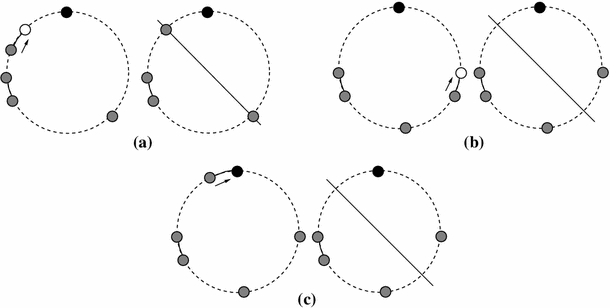

  

  The 3 special types of configurations. A white (grey, black, respectively) circle represents an empty node (a node with one robot, a multiplicity, resp.). A dashed (plain, resp.) arc indicates an arbitrary sequence of empty nodes (two consecutive nodes, resp.). If during the convergence phase a robot should move towards the multiplicity, as indicated by the arrow, then the resulting configuration is at one move from a symmetric configuration with two multiplicities achievable when the algorithm for gathering six robots is applied. The symmetric configurations arise when, in each shown configuration, the two adjacent robots join into a multiplicity

• Conv-s-1 Symmetric configurations with one multiplicity but those on rings of seven nodes with five nodes occupied;

• Conv-a-1 Asymmetric configurations with one multiplicity, but configurations with five nodes occupied on a ring of seven nodes;

  • (a) at one xn move from the symmetry passing through the multiplicity and different from the configurations in Conv-a-s;

  • (b) at more than one move from any symmetry.

The general idea is to gather all the remaining single robots to the only multiplicity by performing xn. However there might occur some exceptions that must be carefully considered. In fact, whenever the gathering leads to configurations with only five nodes occupied, these might be “confused” with configurations in phase multiplicity–convergence obtainable when initially there are only six robots. In order to address such occurrences, we avoid these situations. In particular, the algorithm does not perform an xn move whenever it leads to configurations at one move from a symmetric configuration with two multiplicities achievable when the algorithm for gathering six robots is applied (shown in Fig. 17). These are the configurations in Conv-a-s: in this case we perform another move. That is, we allow again an xn move, but without considering the original robot which was supposed to move. In practice, this equals to move the first robot on the other side of the one planned to move with respect to the multiplicity. It is worth to note that the configurations in Conv-a-s are the only ones to take care of. The other two possible configurations are shown in Fig. 18. After the xn move, they lead to a configuration at one move from a symmetric configuration with two multiplicities, but, in this case, the algorithm in [9] would never generate it and then there is no possible misclassification.

Fig. 18

The two other special asymmetric configurations. After the moves indicated by the arrows the resulting configuration is at one move from a symmetric configuration with two multiplicities, but this symmetric configuration is never generated by the algorithm in [9]

It must be observed that the above method applied from Conv-a-s decreases the number of moves required to move the single robots to the only multiplicity.

From Conv-s-1, the algorithm allows by an xn move the two closest single robots to the multiplicity (or the only remaining one) to move towards the multiplicity. If both make synchronously the move, then the obtained configuration is still in Conv-s-1, but with one move less before the final gathering. If only one robot performs the allowed move, then the configuration is in Conv-a-1. From Conv-a-1 a, either there is only one single robot left, which will be the only one allowed to move towards the multiplicity until the gathering is completed, or there are at least two single robots, each of which has no other robots in between itself and the multiplicity. If the farthest among those two robots re-build the symmetry by one move towards the multiplicity, then it will be the only one allowed to move and the obtained configuration is in Conv-s-1, otherwise the other single robot is the only one allowed to move towards the multiplicity and the obtained configuration might either remain in Conv-a-1 or move to Conv-s-1. Also from Conv-a-1 b, the xn move is performed.

In any case, the number of moves to reach the final gathering is reduced. The pseudo-code of Procedure convergence is given in Fig. 19.

Fig. 19

Procedure convergence

Lemma 8

Phase convergence terminates after a finite number of moves finalizing the gathering or in a configuration in Coll-a-1.

Proof

From the above description, it follows that the graph in Fig. 20 models the execution of phase convergence and that all the cycles are indeed traversed a finite number of times until the gathering is completed. In fact, for each described configuration, one or two robots are allowed to move towards the multiplicity, reducing the number of moves necessary for each single robot to reach the multiplicity. Eventually the gathering is necessarily accomplished. The only exception occurs when a configuration in Conv-a-1 b with more than six nodes occupied leads, after a xn, to a configuration in Coll-a-1 (that is a configuration with one multiplicity at one reduction move from the symmetry). However, this may happen only once as from Coll-a-1 the algorithm achieves configurations with only one multiplicity only if less than six nodes are occupied (for more details, see “From convergence to collect of Appendix 2”). $\square$

Fig. 20

Phase convergence

3.6 Phase seven-nodes

In [9], it has been shown that some configurations with six robots on a ring of seven nodes require special arguments. This phase copes with such cases and it is performed if one of the next configurations occurs:

7N-2:

Configurations with two multiplicities on a ring of seven nodes;

7N-1:

Configurations with one multiplicity and five nodes occupied on a ring of seven nodes.

All the above configurations can occur only when there are six robots on a ring of seven nodes. In fact, for 7N-2 there cannot be initially more than six robots on a ring of seven nodes, and no strategy leads to have two multiplicities apart from the case of six robots. For 7N-1, it may only happen starting from six single robots. In these cases, the algorithm for six robots from [9] is used.

3.7 Selecting the type of configuration

In this section, we show how to recognize the type of configurations among those described above.

We first show that all the above types are pairwise disjoint and that they cover all the possible configurations achieved by the algorithm. Let $\textsc {CTP}= \{$W1, W2, $\ldots$ , W7, Coll-a-1, Coll-a-2, Coll-s-2, Mc-s-x, Mc-a-x, Mc-a-1, Conv-a-s, Conv-a-1, Conv-s-1, 7N-2, 7N-1$\}$ be the set of all the possible configuration types above.

The configurations in $W1$–$W7$ cover all the possible initial configurations in $\mathtt {A}$, as by hypothesis, any initial configuration has no multiplicities. From there, all the configurations in phases collect, multiplicity–convergence, convergence, and seven-nodes can be generated by the algorithm. In the detailed description of each phase, it has been shown that the allowed moves always lead to configurations in CTP. Therefore, the following corollary to Lemmas 5–8 holds.

Corollary 1

All the possible configurations achieved by the algorithm belong to CTP.

Lemma 9

Configuration types in CTP are pairwise disjoint.

Proof

We compare only the configuration types with the same number of multiplicities and degree of symmetry.

The only configuration types with no multiplicities are $W1$–$W7$ and they are clearly pairwise disjoint.

The symmetric configuration types with one multiplicity are in Conv-s-1 and 7N-1 which are disjoint as they differ for the number of nodes or the number of nodes occupied.

The symmetric configuration types with two multiplicities are Coll-s-2 a, Coll-s-2 b, Coll-s-2 c, Mc-s-a, Mc-s-b, and 7N-2 which are disjoint as they differ for the number of nodes or the number of nodes occupied, or the distance between the single robots and the multiplicities. In fact, configurations in Coll-s-2 a are the only ones with more than six nodes occupied. Configurations in Coll-s-2 b are the only ones with six nodes occupied and more than one robot on the north side at distance grater than zero from any multiplicity. This means that in total there is at least one robot on the northern side that must be moved towards its closest multiplicity. This is different from the configurations in Mc-s-b where there are no robots on the northern side at distance greater than zero that must be moved towards the multiplicities as the only robot in such kind of position might only be a guard. Configurations in Coll-s-2 c are the only ones with six nodes occupied and more than two robots at distance grater than zero from the multiplicities. Configurations in Mc-s-a are the only ones with only four nodes occupied on a ring of more than seven nodes. Contrary, configurations in 7N-2 are the only ones with either four or three nodes occupied on a ring of seven nodes.

The asymmetric configuration types with one multiplicity are in Conv-a-s, 7N-1, Coll-a-1, Mc-a-1, Conv-a-1 a, and Conv-a-1 b. Configurations in Conv-a-s are well specified and cannot belong to any other set. Configurations in 7N-1 are the only ones with five nodes occupied on a ring of seven nodes. Configurations in Coll-a-1 are the only ones with six nodes occupied at more than one move from the symmetry passing through the multiplicity but at one pending reduction or xn move from an allowed symmetry. Similarly, configurations in Mc-a-1 are the only ones with five nodes occupied on a ring of more than seven nodes at more than one move from the symmetry passing through the multiplicity but at one pending move according to the algorithm in [9]. Configurations in Conv-a-1 a are the only ones at one xn move from the symmetry passing through the multiplicity, while configurations in Conv-a-1 b are the only ones at more than one move from any allowed symmetry.

The asymmetric configuration types with two multiplicities are in Coll-a-2 a, Coll-a-2 b, Mc-a-a, Mc-a-b, and 7N-2 which are disjoint as they differ for the number of nodes or the number of nodes occupied, or the distances between the single robots and the multiplicities. In fact, configurations in Coll-a-2 a are the only ones with more than six nodes occupied. Configurations in Coll-a-2 b are the only ones with exactly six nodes occupied and at least one single robot -not identified as a guard- at distance greater than zero from any multiplicity, whereas configurations in Mc-a-b are the only ones with exactly six nodes occupied and no single robots -not identified as a guard- at distance greater than zero from any multiplicity. Configurations in Mc-a-a are the only ones with rings of more than seven nodes and less than six nodes occupied. Configurations in 7N-2 are the only ones with rings of seven nodes and less than five nodes occupied.

The remaining configurations can be either asymmetric with three multiplicities, i.e, Mc-a-c, or symmetric configurations with three or four multiplicities, i.e., Mc-s-c and Mc-s-d. $\square$

By the proof of the lemmas above, it follows that, in order to distinguish among the configuration types, it is sufficient to compute, given a configuration $C=(q_0,q_1,\ldots ,q_j)$, the following parameters:

• 1. Number of nodes in the ring, $n(C)$;

• 2. Number of multiplicities, $m(C)$;

• 3. Number of nodes occupied or number of robots in the case without multiplicities, $\omega (C)$;

• 4. Distance between single robots and multiplicities;

• 5. If $C$ is symmetric and in the affirmative case, if the symmetry is allowed;

• 6. If $C$ belongs to Conv-a-s;

• 7. If $C$ is at one move from one of the symmetries allowed by the algorithm.

Parameters 1–3 can be computed by formulas $n(C) = \sum _{q_i\ge 0} (q_i+1)$, $m(C)=|\{i~|~q_i=-1,0\le i\le j\}|$, and $\omega (C) = j +1 - m(C)$, respectively. The distance between single robots and multiplicities is easily computed by summing the intervals between a single robot and a multiplicity. The symmetry of a configuration is computed by procedure $\textsc {symmetric}(C)$. If $C$ belongs to Conv-a-s can be easily checked by comparing all the intervals of $C_i$ and $\overline{(C_i)}$, for each $i\in \{0,1,\ldots ,j\}$ to the configurations in Conv-a-s. To understand whether $C$ is at one move from a symmetry allowed by the algorithm, it is sufficient to simulate such move backwards and checking whether the obtained configuration is symmetric. As an example, to check whether $C$ is at one move from reduction, Procedure check_reduction is used.

3.8 The complete algorithm

In this section, we show how the above phases interact and how the algorithm can switch from one phase to another. We show that starting from any initial configuration among W1–W7, we necessarily end up with configurations in either Conv-a-1 or Conv-s-1 (possibly passing through phases collect and multiplicity–convergence), hence finalizing the gathering.

By Lemmas 5–8, it follows that the interactions between the phases are those given in the graph of Fig. 2. In what follows we show how the edges of such graph are traversed. “Appendix 1” shows in a graphical way all such interactions among configuration types.

The starting configuration can only belong to W1–W7. By Lemma 5, it follows that after a finite number of moves any other phase can be reached. Moreover, once reached a configuration with at least one multiplicity, the algorithm never goes back to configurations without multiplicities, but in the case of six robots. In this latter case in fact, the configurations can swap between those in W3 and those in Mc-a-1 or in Mc-s-x a. However, the number of times that this cycle can be traversed is finite as each time the north interval is reduced, until creating one single multiplicity on the final gathering node (that is, when the system moves to convergence). For more details, see “From multiplicity–convergence to multiplicity–creation of Appendix 2”.

By Lemma 6, phase collect terminates after a finite number of moves in a configuration belonging to phase multiplicity–convergence. In particular, this phase can only terminate with a configuration in Mc-s-x b. In fact, Lemma 6 states that this phase leads to a symmetric configuration with six nodes occupied by two multiplicities, two guards and two single robots adjacent to the multiplicities which defines exactly the configuration type Mc-s-x b.

By Lemma 7, multiplicity–convergence terminates after a finite number of moves in a configuration in phase convergence. In particular, the algorithm can only move from configurations in Mc-s-x a, Mc-s-x c, Mc-a-x a, and Mc-a-1, to configurations in Conv-s-1 and Conv-a-1. In fact, Lemma 7 states that this phase leads to a configuration with one multiplicity and between one and four single robots and, from any other configuration type in multiplicity–convergence, the algorithm leads to a configuration with two multiplicities, eventually. This implies that the last configuration before leaving this phase is in Mc-s-x a, Mc-s-x c, Mc-a-x a, or Mc-a-1. The configuration achieved cannot be in Conv-a-s because this configuration type can be obtained only from a configuration in W3 or in Conv-a-1.

From [9], phase seven-nodes terminate in configurations in convergence.

Finally, from configurations in convergence, the algorithm terminates the gathering with the only exception of the case where a configuration in Conv-a-1 b can lead, after a xn, to a configuration in Coll-a-1 (that is a configuration with one multiplicity at one reduction move from the symmetry). Note that this case can occur only when there are more than six nodes occupied. As the transition from phase multiplicity–convergence to phase convergence can occur only when there are at most six nodes occupied, it follows that the edge between convergence and collect can be traversed only once. For more details, see “From convergence to collect of Appendix 2”.

4 Conclusion

The proposed algorithm answers to the posed conjectures concerning the gathering on the studied model by providing a complete characterization for the initial configurations. The obtained result is of main interest for robot-based computing systems. In fact, it closes all the cases left open with the exception of potentially gatherable configurations in $\mathtt {SP}4$.

Our technique, mostly based on the supermin concept, may result as a new analytical approach for investigating related distributed problems. In fact, the concept of supermin combined with the reduction move can be used to solve other problems in the Look–Compute–Move model such as graph exploration and searching (see e.g [12]). Moreover, similar techniques can be exploited to solve such problems on different graph topologies (see e.g. [8, 11] for the gathering on grids and trees, respectively).

Another challenging direction would be that of investigating the minimum number of steps required by the robots to accomplish the gathering task. So far, the research has mainly focused on the feasibility of the gathering, while few results concern the minimization of the robots’ movements. A first study to this respect can be found in [15]. Similarly, low effort has been spent in order to increase the opportunity to parallelize movements. As we have seen for ring networks, at most two robots are allowed to move concurrently but for the case when the algorithm moves the robots composing multiplicities.

Appendices

Appendix 1: Transitions among types of configuration

In this appendix we provide a graphical representation of the possible transitions among all the types of configurations. In particular, for each configuration type we show all the configurations that can be reached according to the algorithm and the asynchronous execution of the Look–Compute–Move cycles.

Appendix 2: Special cases for configuration transitions

In this section, we describe the behavior of the algorithm in the cases that lead to backward arcs in Fig. 2.

1.1 From multiplicity–convergence to multiplicity–creation

The only case when a configuration in multiplicity–convergence can lead to one of multiplicity–creation is that with six robots, that is the initial configuration was in W3. An exhaustive example is given below.

Let us consider the configuration in Mc-s-x a given in Fig. 21a where each multiplicity contains two robots (and hence there are six robots in the ring). The algorithm aims to move the two multiplicity towards the north. However, it may happen that only one robot moves from each multiplicity, hence obtaining the configuration in W3 given in Fig. 21b. At this point, the algorithm in [9] is applied which leads again to the configuration in Mc-s-x a given in Fig. 21d, possibly passing through that in Fig. 21c which belongs to Mc-a-1. Therefore, in these cases, this process can be repeated a finite number of times, until the two multiplicities join into the north, hence the backward arc from multiplicity–convergence to multiplicity–creation of Fig. 2 can be traversed a finite number of times.

Fig. 21

Configurations on type: (a) Mc-s-x a, (b) W3, (c) Mc-a-1, (d) Mc-s-x a

Fig. 22

Configurations on type: (a) Conv-a-1 b, (b) Coll-a-1, (c) Coll-s-2 c, (d) Mc-s-x a, (e) Conv-s-1

1.2 From convergence to collect

The only case when a configuration in convergence can lead to one of collect is that with more than six nodes occupied where an xn move leads to a configuration at one reduction move from a symmetric configuration. That is we can go from a configuration in Conv-a-1 b to one in Coll-a-1. An exhaustive example is given below.

Let us consider the configuration in Conv-a-1 b given in Fig. 21a. In this case, the algorithm performs an xn move, leading to the configuration given in Fig. 22b. Note that such a configuration belongs to Coll-a-1 as it is at one reduction move from the symmetric configuration in Coll-s-2 c given in Fig. 22c. Therefore, the algorithm forces such a reduction move, obtaining the configuration in Fig. 22c. Then, the two single robots which are not guards are moved to join the multiplicities. At this point (see Fig. 22d) each multiplicity contains at least three robots and therefore both of them are moved towards the north in phase multiplicity–convergence. Since each multiplicity contains at least three robots, this phase cannot generate configurations with only one multiplicity, except for the last steps when the two multiplicities are joint (see e.g. Fig. 22e). This implies that moving from convergence to collect can occur only once and therefore the backward arc from convergence to collect of Fig. 2 can be traversed only once.

References

Alpern, S.: The rendezvous search problem. SIAM J. Control Optim. 33, 673–683 (1995)
Bampas, E., Czyzowicz, J., Gasieniec, L., Ilcinkas, D., Labourel, A.: Almost optimal asynchronous rendezvous in infinite multidimensional grids. In: Proceedings of the 24th Internatioanal Symposium on Distributed Computing (DISC), Lecture Notes in Computer Science, vol. 6343, pp. 297–311 (2010)
Blin, L., Burman, J., Nisse, N.: Exclusive graph searching. In: Proceedings of the 21st Annual European Symposium on Algorithms (ESA), Lecture Notes in Computer Science, vol. 8125, pp. 181–192 (2013)
Blin, L., Milani, A., Potop-Butucaru, M., Tixeuil, S.: Exclusive perpetual ring exploration without chirality. In: Procedings of the 24th International Symposium on Distributed Computing (DISC), Lecture Notes in Computer Science, vol. 6343, pp. 312–327. Springer (2010)
Chalopin, J., Das, S.: Rendezvous of mobile agents without agreement on local orientation. In: Proceedings of the 37th International Conference on Automata, Languages and Programming (ICALP), Lecture Notes in Computer Science, vol. 6199, pp. 515–526 (2010)
Cord-Landwehr, A., Degener, B., Fischer, M., Hüllmann, M., Kempkes, B., Klaas, A., Kling, P., Kurras, S., Märtens, M., Der Heide, F.M.A., Raupach, C., Swierkot, K., Warner, D., Weddemann, C., Wonisch, D.: A new approach for analyzing convergence algorithms for mobile robots. In: Proceedings of the 38th International Conference on Automata, Languages and Programming (ICALP), Lecture Notes in Computer Science, vol. 6756, pp. 650–661 (2011)
Czyzowicz, J., Labourel, A., Pelc, A.: How to meet asynchronously (almost) everywhere. In: Proceedings of the 21st ACM-SIAM Symposium on Discrete Algorithms (SODA), pp. 22–30 (2010)
D’Angelo, G., Di Stefano, G., Klasing, R., Navarra, A.: Gathering of robots on anonymous grids without multiplicity detection. In: Proceedings of the 19th International Colloquium on Structural Information and Communication Complexity (SIROCCO), Lecture Notes in Computer Science, vol. 7355, pp. 327–338 (2012)
D’Angelo, G., Di Stefano, G., Navarra, A.: Gathering of six robots on anonymous symmetric rings. In: Proceedings of the 18th International Colloquium on Structural Information and Communication Complexity (SIROCCO), Lecture Notes in Computer Science, vol. 6796, pp. 174–185 (2011)
D’Angelo, G., Di Stefano, G., Navarra, A.: How to gather asynchronous oblivious robots on anonymous rings. In: Proceedings of the 26th International Symposium on Distributed Computing (DISC), Lecture Notes in Computer Science, vol. 7611, pp. 330–344 (2012)
D’Angelo, G., Di Stefano, G., Navarra, A.: Gathering asynchronous and oblivious robots on basic graph topologies under the look–compute–move model. In: S. Alpern, R. Fokkink, L. Gasieniec, R. Lindelauf, V. Subrahmanian (eds.) Search Theory: A Game Theoretic Perspective, pp. 197–222. Springer, Berlin (2013)
D’Angelo, G., Di Stefano, G., Navarra, A., Nisse, N., Suchan, K.: A unified approach for different tasks on rings in robot-based computing systems. In: Proceedings of the 15th IEEE IPDPS Workshop on Advances in Parallel and Distributed Computational Models (APDCM), pp. 667–676 (2013)
Degener, B., Kempkes, B., Langner, T., Meyer auf der Heide, F., Pietrzyk, P., Wattenhofer, R.: A tight runtime bound for synchronous gathering of autonomous robots with limited visibility. In: Proceedings of the 23rd ACM Symposium on Parallelism in Algorithms and Architectures (SPAA), pp. 139–148 (2011)
Dessmark, A., Fraigniaud, P., Kowalski, D., Pelc, A.: Deterministic rendezvous in graphs. Algorithmica 46, 69–96 (2006)
Di Stefano, G., Navarra, A.: Optimal gathering of oblivious robots in anonymous graphs. In: Proceedings of the 20th International Colloquium on Structural Information and Communication Complexity (SIROCCO), Lecture Notes in Computer Science, vol. 8179, pp. 213–224 (2013)
Flocchini, P., Ilcinkas, D., Pelc, A., Santoro, N.: Remembering without memory: tree exploration by asynchronous oblivious robots. Theor. Comput. Sci. 411(14–15), 1583–1598 (2010)
Flocchini, P., Ilcinkas, D., Pelc, A., Santoro, N.: Computing without communicating: ring exploration by asynchronous oblivious robots. Algorithmica 65(3), 562–583 (2013)
Flocchini, P., Prencipe, G., Santoro, N., Widmayer, P.: Gathering of asynchronous robots with limited visibility. Theor. Comput. Sci. 337, 147–168 (2005)
Izumi, T., Izumi, T., Kamei, S., Ooshita, F.: Randomized gathering of mobile robots with local-multiplicity detection. In: Proceedings of the 11th International Symposium on Stabilization, Safety, and Security of Distributed Systems (SSS), Lecture Notes in Computer Science, vol. 5873, pp. 384–398 (2009)
Izumi, T., Izumi, T., Kamei, S., Ooshita, F.: Mobile robots gathering algorithm with local weak multiplicity in rings. In: Proceedings of the 17th International Colloquium on Structural Information and Communication Complexity (SIROCCO), Lecture Notes in Computer Science, vol. 6058, pp. 101–113 (2010)
Kamei, S., Lamani, A., Ooshita, F., Tixeuil, S.: Asynchronous mobile robot gathering from symmetric configurations. In: Proceedings of the 18th International Colloquium on Structural Information and Communication Complexity (SIROCCO), Lecture Notes in Computer Science, vol. 6796, pp. 150–161 (2011)
Kamei, S., Lamani, A., Ooshita, F., Tixeuil, S.: Gathering an even number of robots in an odd ring without global multiplicity detection. In: Proceedings of 37th International Symposium on Mathematical Foundations of Computer Science (MFCS), LNCS, vol. 7464, pp. 542–553 (2012)
Klasing, R., Kosowski, A., Navarra, A.: Taking advantage of symmetries: gathering of many asynchronous oblivious robots on a ring. Theor. Comput. Sci. 411, 3235–3246 (2010)
Klasing, R., Markou, E., Pelc, A.: Gathering asynchronous oblivious mobile robots in a ring. Theor. Comput. Sci. 390, 27–39 (2008)
Koren, M.: Gathering small number of mobile asynchronous robots on ring. Zeszyty Naukowe Wydzialu ETI Politechniki Gdanskiej. Technologie Informacyjne 18, 325–331 (2010)
Suzuki, I., Yamashita, M.: Distributed anonymous mobile robots: formation of geometric patterns. SIAM J. Comput. 28(4), 1347–1363 (1999)
Yamashita, M., Souissi, S., Défago, X.: Gathering two stateless mobile robots using very inaccurate compasses in finite time. In: Proceedings of the 1st International Conference on Robot Communication and Coordination (RoboComm), pp. 48:1–48:4 (2007)
Author information
Authors and Affiliations
Corresponding author
Additional information
Work supported by the Research Grant 2010N5K7EB ‘PRIN 2010’ ARS TechnoMedia (Algoritmica per le Reti Sociali Tecno-mediate) from the Italian Ministry of University and Research. Preliminary results concerning this work have been presented in [10].