Monodomain response of finite-aspect-ratio macromolecules in shear and related linear flows

Abstract.

Recent extensions of the Doi kinetic theory for monodisperse nematic liquids describe rigid, axisymmetric, ellipsoidal macromolecules with finite aspect ratio. Averaging and presumed linear flow fields provide tensor dynamical systems for mesoscopic, bulk orientation response, parameterized by molecular aspect ratio. In this paper we explore phenomena associated with finite vs infinite aspect ratios, which alter the most basic features of monodomain attractors: steady vs unsteady, in-plane vs out-of-plane, multiplicity of attracting states, and shear-induced transitions. For example, the Doi moment-closure model predicts a period-doubling cascade in simple shear to a chaotic monodomain attractor for aspect ratios around 3:1 or 1:3, similar to full kinetic simulations by Grosso et al. [Grosso M, Keunings R, Crescitelli S, Maffettone PL (2001), Prediction of chaotic dynamics in sheared liquid crystalline polymers. Preprint (2001) and lecture, Society of Rheology Annual Meeting, Hilton Head, SC, February 2001] for infinite aspect ratios. We develop symmetries of mesoscopic tensor models robust to closure approximations but specific to linear flow fields, and analytical methods to determine:

• The entire monodomain phase diagram of a finite-aspect-ratio nematic fluid in a linear flow field is equivalent to the phase diagram of an infinite-aspect-ratio fluid (thin rods or discs) in a related linear velocity field.

• Rod-like and discotic macromolecules with reciprocal aspect ratios have equivalent bulk shear response, related by a simple director transformation.

• Out-of-plane, shear-induced monodomains (steady and transient) either are symmetric about the shearing plane (e.g., logrolling and kayaking modes), or occur in pairs mirror-symmetric about the shearing plane (out-of-plane steady and periodic "tilted kayaking" modes), revealing a symmetry mechanism for bi-stability.

• A tensor analog of the Leslie alignment vs tumbling criterion, which is developed and applied to predict the multiplicity, stability, and steady or transient property of shear-induced monodomains.

Simulations highlight the degree to which scaling properties of Leslie-Ericksen theory are violated. By varying molecular aspect ratio, any shear-induced monodomain is reproducible among the well-known closure approximations, yet no single closure rule suffices to capture all known attractors and transition scenarios.

Introduction

Theoretical and numerical studies of homogeneous responses of nematic polymers and liquid crystals to simple shear (Fig. 1) have spanned four decades; a representative yet inexhaustive list is [4, 5, 14, 21, 22, 24, 26, 27, 30, 33, 40, 41, 43, 44, 45, 63, 65, 66, 67, 68, 69, 70, 80, 82, 83, 85, 86, 90, 91, 92, 93, 94, 95, 96, 97, 100, 101, 118, 119, 120, 124, 125, 126, 127, 128, 132, 133, 136, 137, 138, 146], contributing to a fundamental understanding of macromolecular fluids. These studies aspire to reproduce, explain, and predict experimental discoveries of monodomain behavior, e.g., [1, 6, 7, 12, 13, 16, 17, 19, 20, 35, 36, 37, 59, 61, 64, 78, 79, 98, 106, 107, 108, 109, 110, 112, 114, 115, 116, 117, 121, 122, 129, 130, 142, 143, 144]. Experimental imaging that allows comparison with theory has been enabled by advances in shear devices and rheo-optics, e.g., [12, 58, 73].

Fig. 1.

The shear flow geometry, where υ₀ is the velocity of the moving plate: $\upsilon _0 = \dot \gamma \times$ (width-between-the-plates)

By a combination of theory and experiment, many steady and transient shear-induced, monodomain modes have been catalogued and named primarily on the basis of director response: steady alignment with primary director either in the shear plane (flow aligning) or along the vorticity axis (logrolling); in-plane transient oscillatory (wagging) or rotating (tumbling) director modes; and out-of-plane transient director modes (kayaking). Complicated dynamics is also possible. Recent full kinetic simulations of the Doi theory for monodomains [63] of rigid rods indicate a shear window of highly erratic director motions, i.e., homogeneous director "temporal chaos", in contrast with the "spatial chaos" referred to as director turbulence at least two decades ago (e.g., [99]). (The thesis of Edwards [39] contains numerical evidence of chaotic behavior in the tensor models of Beris and Edwards [10]; refer also to graphical evidence in [3]).

We show below that these temporal chaotic attractors are resolved with simple Doi closure models. The kinetic simulations of [63] establish a period-doubling route to chaos, with the underlying orbit an out-of-plane periodic state; the Doi model with finite aspect ratio reproduces this scenario! Often it is possible to understand chaotic attractors in terms of a symbol sequence. We give graphical evidence that the erratic dynamics is related to a random switching between metastable attractors, consistent with kinetic simulations [55, 63].

We pay particular attention to dynamics of the degrees of orientation that accompany director motions. This feature of mesoscopic tensor theories [10, 33, 34, 68, 97, 124] addresses behavior that is not captured from traditional L-E models. The a priori consequences of a restricted, single-director theory will be consistently highlighted.

The characterization of monodomain shear response and all shear-rate-dependent transitions is routinely utilized, for example:

• For fundamental rheological classification of given nematic polymers [30] (e.g., "flow-aligning 5CB" [107] vs "tumbling 8CB" [108])

• Transitions between monodomain attractors (e.g., the tumbling to flow-aligning transition) correlate with measurable sign changes in first and second normal stress differences [78, 79, 82, 83, 85, 92, 100, 101, 102, 126]

• As a precursor and indicator of subsequent formation of spatial structures and textures [12, 20, 130]

We refer to two important review papers by Marrucci and Greco [105] and Burghardt [18] for discussions of the rheological responses of sheared nematic polymers, and in particular the correlations between texture formation and monodomain modes for several different (flow-aligning vs tumbling) nematic fluids.

Below we will focus on transition phenomena in several tensor models; the effect of finite molecular aspect ratio will appear prominently. In a subsequent study [56] we follow many investigations into structure formation in processing-type flows which are well-approximated by linear flow fields. One of our motivations here is to have tensor models with sufficient flexibility to be able to characterize bulk monodomain response for a laboratory nematic liquid. The role of finite aspect ratio is shown in this paper to enrich the flow-phase diagrams of infinite-aspect-ratio tensor models, thereby being capable of reproducing far more features of full kinetic simulations.

It is standard protocol to infer tumbling vs non-tumbling nematics from the laboratory by the structure of normal stress differences and apparent viscosity versus shear rate, clarified and developed in various laboratories ([11, 16, 18, 20, 61, 62, 72, 73, 84, 87, 88, 89, 98, 113, 114, 117, 130, 131, 142, 144, 145]). Many experimental studies now routinely include model simulations, still dominated by Leslie-Ericksen theory. Likewise, it is required protocol for theorists to identify shear-driven phase transitions, and to classify the precise nature of those transitions so they may be confirmed or not by experiment. The explicit characterization of phase transitions in terms of bifurcation type has its roots in the work of Hess [68], Semenov [126], Kuzuu and Doi [82, 83], Edwards and coworkers [38, 39], Marrucci and Maffettone [100], and Larson [85], and now has become a routine tool for identifying and classifying bifurcations (e.g., [2, 3, 14, 25, 43, 44, 48, 50, 65, 66, 93, 96, 123, 128, 139]).

Bifurcation analysis illuminates qualitative features of monodomains at shear rates just below or above phase transitions. We are interested in which orientation features (in-plane vs out-of-plane components, directors vs degrees of orientation) inherit the dynamics associated with bifurcations. The graphics presented illustrate that one cannot a priori anticipate whether monodomain attractors are director-dominated or order-parameter-dominated; refer to the dynamics of tumbling vs wagging attractors, for example. We further refer the reader to mathematical treatments [25, 60, 135] which apply equivariant bifurcation theory as well as normal form analysis to explain symmetric patterns and certain monodomain transition phenomena. The heterogeneous patterns are related to our own constructions [49, 51], but they exploit symmetries of tensor equations in a systematic way. These powerful tools have only started to be applied toward nematic structure properties, where a host of space-time bifurcation phenomena await discovery. For example, the uniaxial planar analysis of the tumbling-wagging transition by Farhoudi and Rey [44] is extended to biaxial in-plane tensors [25, 135], which identifies this transition with a Takens-Bogdanov bifurcation phenomenon.

The question of bifurcation type, and what bifurcations are possible, amplifies the issue of two-dimensional (director) vs five-dimensional (tensor) models for monodomains. Two-dimensional autonomous dynamical systems cannot produce the complex dynamics revealed here. Some critical a priori differences are:

• L-E theory guarantees a scaling property that allows superposition of data for any constant shear rate into a master curve in units of strain [18, 90, 91, 105, 144]. Small molecule liquid crystals appear to obey accurately this scaling law (e.g., [134]), as well as recent data [144] for in-plane shear alignment of certain main-chain thermotropes.

• The Doi [34], Hess [68], Landau-deGennes [30], or Beris-Edwards [10] mesoscopic tensor theories do not share this scaling property, as detailed below, essentially because of order parameter variation induced by the short-range, excluded-volume potential.

• There are no shear-rate-dependent monodomain transitions in L-E models, only viscosity-dependent transitions! Yet the tumbling-to-alignment transition is observed in tumbling nematics at a critical shear rate. The only way one can model such behavior with L-E theory is to posit shear-rate-dependent viscosities. By contrast, the full tensor theory admits a diversity of bifurcations vs shear rate for a fixed nematic liquid; moreover, these transitions dominate the weak flow regime for finite aspect ratios, and the predictions are highly sensitive to the tensor model one chooses.

• Chaotic dynamics is not possible in planar autonomous systems, yet overwhelming evidence exists from Doi molecular theory [55, 63] and even from experiments [8, 13, 111] that chaotic bulk motions exist.

The current paper tests predictions of the recent extended Doi kinetic model of Wang [140], applied to shear-induced bulk behavior of finite-aspect-ratio, monodisperse, nematic liquids. Recent work of Singh and Rey [128], Rienacker and Hess [124], and Maffettone et al. [97] also explicitly models finite-aspect-ratio, axisymmetric ellipsoidal molecules in Doi, Hess, and Landau-deGennes tensor models. To our knowledge, ours is the first systematic study of the role of finite aspect ratio in mesoscopic tensor models of monodomain responses to shear. The methods we develop are not specific to the class of tensor models.

We first summarize the modern Doi kinetic theory and the mesoscopic orientation tensor model that follows, prior to closure approximation. Four popular closure rules are then recalled. Our new results begin with symmetry properties of the mesoscopic theory that are independent of closure approximation, together with experimental implications of these symmetry properties. We then develop a tensor version of a Leslie alignment-vs-tumbling criterion, and study the selection mechanism of steady and periodic monodomains in the weak shear limit. Our weak-shear analysis is equivalent to that of Maffettone et al. [97] who studied a particular Landau-deGennes tensor model, and identify their model with a specific parameter regime and closure approximation of Doi kinetic theory. A similar in-plane tensor analysis is also given by Rienacker and Hess [124] from a second-moment closure approximation of Hess kinetic theory.

Our analysis explains the multiplicity, stability, and steady vs unsteady nature of monodomain solutions in simple shear. The methods also reveal the remarkable sensitivity of these monodomain selection criteria vs shear rate, both to closure rule (equivalently, which tensor model one chooses) and to molecular aspect ratio. We then, following seminal studies of Maffettone and his collaborators, use continuation software packages to track solution branches in the multi-parameter space of shear rate, molecular aspect ratio, and closure rule. For this paper we restrict to a high nematic concentration N=6, well into the stable nematic regime, which removes further complexity associated with the I-N transition.

After recalling infinite aspect ratio results, we focus on behavior associated with a finite molecular aspect ratio in the range 3:1 to 20:1 for rod-like (prolate) or disc-like (oblate) axisymmetric ellipsoidal molecules. We then proceed to the primary quantitative results of each closure model, i.e., detailed flow-phase bifurcation diagrams. The dramatic role of aspect ratio is illustrated in various ways. We shall show that previously determined "failures" of the Doi closure are repaired with the added role of a finite aspect ratio. Thus the problems noted in the literature (e.g., failure to capture important steady-unsteady transitions, tumbling, wagging, or kayaking behavior) are not the consequence of the Doi closure approximation. Given these observations, it seems prudent to revisit previous conclusions drawn from closure rules with infinite aspect ratio; we do so for four different closures, with and without orientation-dependent rotary diffusivity. Some features and models are robust to the form of rotational diffusivity, others are not.

Kinetic theory and mesoscopic models for finite-aspect-ratio nematic fluids

We briefly review the homogeneous form of the Doi-type kinetic model of Wang [140] only to the extent necessary to reproduce results of this paper. We assume nematic polymer liquids consisting of monodisperse, rigid, axisymmetric ellipsoidal molecules immersed in a viscous solvent. Such molecules are uniquely characterized by an axis of symmetry, m, and an aspect ratio r of the length along the symmetry axis divided by the radius of the transverse circular cross-section. Infinitely thin rods, spheres, and infinitely thin discs correspond to $r = \infty ,\;1,\;0$ , respectively. This kinetic model shares features with several other models (e.g., [46, 81, 82, 83, 133]), including molecular geometry, orientation-dependent rotary diffusivity, excluded-volume effects, and distortional elasticity potentials of Marrucci and Greco [103, 104, 105]. The latter effects do not come into play for monodomain dynamics addressed here, but are essential for subsequent morphology formation; e.g., the highly disparate elasticity constants for rod-like vs discotic nematics do not enter here. Once the kinetic model is summarized, we discuss four closure approximations that yield simplified approximate models.

Let f (m,x,t) be the distribution function corresponding to the probability that the axis of revolution of the molecule is parallel to direction ${\bf m}\left( {||{\bf m}|| = 1} \right)$ at location x and time t. The fluid velocity is denoted v. The Smoluchowski (kinetic) equation for f(m,x,t), neglecting translational diffusion as is customary, is given by (e.g., [15, 30, 34]):

$${{Df} \over {Dt}} = {\cal R} \cdot [D_r ({\bf m},a)({\cal R}f + {1 \over {kT}}f{\cal R}V_{MS} )] - {\cal R} \cdot [{\bf m} \times {\bf \dot m}f],$$

(1)

where ${\textstyle{D \over {Dt}}}( \bullet )$ denotes the material derivative ${\textstyle{\partial \over {\partial t}}}( \cdot ) + {\bf v} \cdot \nabla ( \cdot )$ , ${\textstyle{\partial \over {\partial {\bf x}}}} = \nabla$ and ${\cal R} = {\bf m} \times {\textstyle{\partial \over {\partial {\bf m}}}}$ are the spatial and the rotational gradient operator, respectively;

$${\bf \dot m} = \Omega \cdot {\bf m} + a[{\bf D} \cdot {\bf m} - {\bf D}:{\bf mmm}]$$

(2)

is the Jeffery orbit of ellipsoids [74], D and Ω are the rate of strain and vorticity tensors, defined by (with the convention $(\nabla {\bf v})_{ij} = {\textstyle{{\partial v_i } \over {\partial x_j }}}$ )

$${\bf D} = {1 \over 2}(\nabla {\bf v} + \nabla {\bf v}^T ),\;\Omega = {1 \over 2}(\nabla {\bf v} - \nabla {\bf v}^T ),\;$$

(3)

where –1≤ a≤ 1 is the molecular shape parameter related to the molecular aspect ratio r by

$$a = {{r^2 - 1} \over {r^2 + 1}}.$$

(4)

Note that a≈1corresponds to the thin rod limit; a=0 corresponds to spherical molecules; and a≈–1 corresponds to the thin disc limit. The rotary diffusion coefficient in Eq. (1) is defined by

$$D_r ({\bf m},a) = \hat D_r (a)(\int_{\left\| {{\bf m}\prime } \right\| = 1} \left\| {{\bf m} \times {\bf m}\prime } \right\|f({\bf m}\prime ,{\bf x},t)d{\bf m}\prime )^{ - 2} ,$$

(5)

where the pre-factor $\hat D_r (a)$ is a (possibly aspect-ratio-dependent) rotary diffusion constant, k is the Boltzmann constant, T is the absolute temperature, and V _MS is the Maier-Saupe intermolecular potential with strength proportional to the dimensionless polymer concentration N:

$$ V_{MS} = - {{3NkT} \over 2} \left\langle {{\bf mm}} \right\rangle :{\bf mm}. $$

(6)

Averaged mesoscopic orientation of the nematic molecules m is captured by

$${\bf M} = \left\langle {{\bf mm}} \right\rangle = \int_{\left\| {\bf m} \right\| = 1} {\bf mm}f({\bf m},{\bf x},t)d{\bf m},$$

(7)

the second moment of m with respect to the probability density function (pdf). Traditionally, one normalizes M to have zero trace, and

$${\bf Q} = \left\langle {{\bf mm}} \right\rangle - {{\bf I} \over 3}$$

(8)

is called the orientation tensor. M and Q share an orthonormal frame of eigenvectors, called the directors or optical axes, with corresponding eigenvalues d _i ,i=1, 2, 3 of M, EquationSource % MathType!MTEF!2!1!+- % feaaeaart1ev0aqatCvAUfeBSjuyZL2yd9gzLbvyNv2CaerbuLwBLn % hiov2DGi1BTfMBaeXatLxBI9gBaerbd9wDYLwzYbItLDharqqtubsr % 4rNCHbGeaGqiVu0Je9sqqrpepC0xbbL8F4rqqrFfpeea0xe9Lq-Jc9 % vqaqpepm0xbba9pwe9Q8fs0-yqaqpepae9pg0FirpepeKkFr0xfr-x % fr-xb9adbaqaaeGaciGaaiaabeqaamaabaabaaGcbaGaamizamaaBa % aaleaacaWGPbaabeaakiabgkHiTmaaleaaleaacaaIXaaabaGaaG4m % aaaaaaa!3A78!$d_i - {\textstyle{1 \over 3}}$ of Q, called the order parameters where

$$ \matrix{ {d_i = \left\langle {({\bf m} \cdot {\bf n}_i )^2 } \right\rangle ,} \hfill \cr {d_1 + d_2 + d_3 = 1,} \hfill \cr {{\bf Q} = \sum\limits_{i = 1}^3 \,(d_i - {1 \over 3}){\bf n}_i {\bf n}_i .} \hfill \cr } $$

(9)

Each 0≤d _i≤1 conveys the degree to which the mesoscale ensemble of molecules m is aligned with respect to the primary director n _i. Geometrically M or Q uniquely defines an orientation ellipsoid whose semi-axes are prescribed by the directors n _i and whose axis lengths are the respective degrees of orientation d _i. Furthermore, spatial homogeneity grants that we can completely specify all monodomain solutions by steady or time-lapse visualization of the ellipsoids relative to the shear flow and flow gradient directions. This imaging of monodomains has been utilized by many authors; we refer to the review by Marrucci and Greco [105] for a compelling discussion. The reader may refer forward to Figs. 3, 4, and 5 for the mesoscale ellipsoids associated with Q(t). We further extract from the ellipsoid the director motion on the sphere (the major director alone would be akin to an L-E simulation) [128], and the order parameter motion (which measures departure from L-E theory). Similar to the L-E continuum theory, the second-moment tensor mimics the molecular geometry at the mesoscopic scale: the axisymmetric ellipsoidal molecule becomes (upon averaging) a full ellipsoid with three distinct semi-axes lengths d _i.

The maximum normalized birefringence is the maximum of $|d_i - d_j |$ , occurring in the plane of n _i, n _j. The nematic is: biaxial if the d _i are distinct; uniaxial if d _i=d _j≠d _k, in which case the director n _k of the simple eigenvalue d _k is "the" director; and isotropic if all $d_i = {\textstyle{1 \over 3}}$ , i.e., Q=0. The major director is defined as n _k for which d _k is the unique maximum. By comparison, the Leslie-Ericksen continuum theory corresponds to two restrictions on the tensor Q: uniaxiality (i.e., a unique director), and the molecule axis is identical with the director. These translate to fixing the d _i at values 1, 0, 0 which removes two degrees of freedom, and losing one director degree of freedom in the isotropic plane transverse to the director.

A dynamical equation for the orientation tensor Q is derived by taking the second moment of m with respect to the pdf f, then using the kinetic equation (Eq. 1) and Jeffery molecule dynamics (Eq. 2):

$$ \left\{ {\matrix{ {{D \over {Dt}}{\bf Q} - \Omega \cdot {\bf Q} + {\bf Q} \cdot \Omega - a[{\bf D} \cdot {\bf Q} + {\bf Q} \cdot {\bf D}] = {{2a} \over 3}{\bf D} - 2a{\bf D}:\left\langle {{\bf mmmm}} \right\rangle } \hfill \cr { - 6D_r^0 [{\bf Q} - N({\bf Q} + {{\bf I} \over 3}) \cdot {\bf Q} + N{\bf Q}:\left\langle {{\bf mmmm}} \right\rangle ],} \hfill \cr } } \right. $$

(10)

where

$$D_r^0 = \left\{ {\matrix{ {{{\tilde D_r^0 } \over {(1 - {\textstyle{3 \over 2}}{\bf Q}:{\bf Q})^2 }},} \hfill & {{\rm with}\;{\rm orientation - dependent}\;{\rm rotary}\;{\rm diffusivity},} \hfill \cr {\tilde D_r^0 ,} \hfill & {{\rm without}\;{\rm orientation - dependent}\;{\rm rotary}\;{\rm diffusivity},} \hfill \cr } } \right.$$

(11)

where $\tilde D_r^0$ is a constant averaged rotary diffusivity that results from the averaging process [34].

For future purposes of monitoring the first and second normal stress differences, we record the homogeneous stress tensor (apart from an isotropic pressure):

$$\matrix{ {\tau = (2\eta + 3ckT\zeta _3 (a)){\bf D} + 3a\nu kT[{\bf Q} - N({\bf Q} + {{\bf I} \over 3}){\bf Q} + N{\bf Q}:\left\langle {{\bf mmmm}} \right\rangle ]} \hfill \cr { + 3\nu kT[\zeta _1 (a)({\bf DM} + {\bf MD}) + \zeta _2 (a){\bf D}:\left\langle {{\bf mmmm}} \right\rangle ],} \hfill \cr } $$

(12)

where η is the solvent viscosity, ζ_1,2,3 (a) are three shape-dependent friction coefficients given in the Appendix, and v is the number density of LCP molecules per unit volume. The quantities 3vkTζ_i, i=1,2,3 are Doi analogs of Leslie viscosities.

These equations, coupled with momentum, mass, and energy balance equations, constitute the modified Doi equations for nematic polymer fluids. For isothermal, linear flow fields, these conservation laws are satisfied identically, and the full system "simplifies" to the homogeneous orientation tensor dynamics governed by Eq. (10). However, the presence of fourth-order tensors in Eq. (10) and the extra stress (Eq. 12) couples the second-moment evolution equation to fourth-moments, requiring one either to continue to generate higher moment equations and truncate at some finite order, or to solve the Smoluchowski equation (Eq. 1) directly, as in [43, 53, 54, 55, 63, 86, 93, 96]. To avoid this computational and analytical complexity, many authors have introduced closure approximations, a tack which we follow in this paper. Alternatively, one can posit Landau-deGennes [29, 68] or Beris-Edwards-Grmela [10] mesoscopic tensor models, all of which can be identified as a particular choice of closure rule from the Hess or Doi kinetic theory together with a particular form of the intermolecular potential and molecular aspect ratio. One example (the Rey-Tsuji model) is illustrated below, two others in [97, 124]. As emphasized by de Gennes [29] and Hess [68], and further discussed by Marrucci and Greco [105], whatever mesoscopic tensor model one posits, the system should retain the fundamental orientational degeneracy property of nematic polymers; i.e., without any applied field, the directions of orientation should be invariant under the full orthogonal group of rotations. We now recall four well-known closure approximations that have been effective in specific applications:

• Quadratic (Doi) closure:

  $$( \bullet ):\left\langle {{\bf mmmm}} \right\rangle \approx ( \bullet ):{\bf MM},$$

  (13)

where $( \bullet )$ is any second order tensor.

• Rey-Tsuji (RT) closure (Rey and Tsuji [133] employed the rule):

  $$ \matrix{ {( \bullet ):\left\langle {{\bf mmmm}} \right\rangle \approx {1 \over 4}[( \bullet ):{\bf QQ} + ( \bullet ){\bf Q}^2 + {\bf Q}( \bullet ){\bf Q} + {\bf Q}^2 ( \bullet )} \hfill \cr { - (( \bullet ){\bf Q}):{\bf QI}] + {1 \over 3}(( \bullet ):{\bf Q} + {{\rm 1} \over {\rm 3}}){\bf I}.} \hfill \cr } $$

  (14)

Hinch and Leal developed two closure approximations in their studies of suspension rheology [71].

• Hinch-Leal 1 (HL1) closure:

  $$\matrix{ {( \bullet ):\left\langle {{\bf mmmm}} \right\rangle \approx {1 \over 5}[6{\bf M}( \bullet ){\bf M} - {\bf MM}:( \bullet ) - } \hfill \cr {2({\bf MM}):( \bullet ){\bf I} + 2{\bf M}:( \bullet ){\bf I}].} \hfill \cr } $$

  (15)

• Hinch-Leal 2 (HL2) closure:

  $$\matrix{ {( \bullet ):\left\langle {{\bf mmmm}} \right\rangle \approx {\bf M}({\bf M}:( \bullet )) + 2[{\bf M}( \bullet )} \hfill \cr {{\bf M} - ({\bf M})^2 ({\bf M}^2 :( \bullet ))/({\bf I}:({\bf M}^2 ))] + } \hfill \cr {\alpha ({\bf M})[{{52} \over {315}}( \bullet ) - {8 \over {21}}[( \bullet ){\bf M} + {\bf M}( \bullet ) - {2 \over 3}({\bf M}:( \bullet )){\bf I}]],} \hfill \cr } $$

  (16)

where

$$\alpha ({\bf M}) = exp[2({\bf I} - 3{\bf M}^2 :{\bf I})/({\bf I} - {\bf M}^2 :{\bf I})].$$

(17)

These closure approximations have been used in the Doi theory with infinite aspect-ratio ($|a| = 1$ ) in both simple shear [24, 86, 133, 138] and extensional flows [48, 50, 123, 139] and even more complex geometries [45]. A general conclusion would be that there is no clear best closure for all flows and flow rates. For example, the quadratic closure gives reasonable predictions in strong (elongational) flows [48, 51, 123, 139] and flows with a slight stretching [24]; the HL-2 closure is superior with respect to the tumbling parameter vs equilibrium order parameter comparisons with the full kinetic theory [71, 85]. To our knowledge, no systematic evaluation of closure rules has been performed for shear-driven flows of finite-aspect-ratio macromolecules. Such a study seems especially warranted due to the significant qualitative changes in each closure model induced by finite versus infinite molecular geometry. Singh and Rey [128] compared closures at the finite discotic ratio $r = {\textstyle{1 \over 3}}$ .

These closure rules may each be applied with constant rotary diffusivity (Eq. 21b) and with orientation-dependent rotary diffusivity (Eq. 21a). The following prescriptions have been used in the references above, providing the model systems we now analyze:

• Modified Doi Model: the quadratic closure is applied everywhere for $( \bullet ):\left\langle {{\bf mmmm}} \right\rangle \rangle$ .

• Doi-Rey-Tsuji Model: the quadratic closure is applied to M: 〈mmmm〉 in the orientation tensor equation, and the Rey-Tsuji closure is used for all other terms. (Note that this identification shows that the Rey-Tsuji model is equivalent to the Doi theory with a specific closure, which has not been observed previously in the literature. This point is important, as noted in the Conclusion, regarding choices of second-order tensor models with distortional elasticity for the purposes of simulating and modeling structure formation. Closures strongly affect monodomain selection criteria, and therefore can be expected to strongly affect structure evolution [56].)

• Modified Doi-Hinch-Leal Models: the quadratic closure is applied to M: 〈mmmm〉 in the orientation tensor equation, and the H-L1 or H-L2 closure is applied for all other fourth-order moment terms.

Monodomain responses to linear flows with a shear component

We begin by noting two important correspondences that follow from the Doi mesoscopic theory: one between finite and infinite aspect-ratio nematic fluids in related linear flow fields, and the other between rod-like and discotic molecules in the same linear flow field. These properties are independent of closure approximation, and therefore follow for all of the models we analyze in the next two sections.

We are primarily concerned with simple steady shear flow in Cartesian coordinates (x, y, z) with constant shear rate $\dot \gamma$ :

$${\bf v}_{shear} = \dot \gamma (y,0,0).$$

(18)

The shear timescale t _s=$\dot \gamma$ ^–1 competes with the average nematic relaxation timescale, $t_n = {\textstyle{1 \over {6\tilde D_r^0 }}}$ , which we presume to be fixed for a given nematic fluid. We nondimensionalize Eq. (10) in nematic relaxation time units:

$$\matrix{ {{\partial \over {\partial \tilde t}}{\bf Q} - Pe[\tilde \Omega \cdot {\bf Q} - {\bf Q} \cdot \tilde \Omega + a({\bf \tilde D} \cdot {\bf Q} + {\bf Q} \cdot {\bf \tilde D})] = aPe[{2 \over 3}{\bf \tilde D} - 2{\bf \tilde D}:\left\langle {{\bf mmmm}} \right\rangle ]} \hfill \cr { - {1 \over \Lambda }[{\bf Q} - N({\bf Q} + {1 \over 3}{\bf I}) \cdot {\bf Q} + N{\bf Q}:\left\langle {{\bf mmmm}} \right\rangle ],} \hfill \cr } $$

(19)

where $\tilde t = {t \over {t_n }}$ and the Peclet number

$$Pe = t_n \dot \gamma $$

(20)

is the shear rate normalized by the average rate of rotational diffusivity. (Note: this ratio also defines a Deborah number, e.g., [18, 88].) The dimensionless rotary diffusion is then

$$\Lambda = \left\{ {\matrix{ {\left( {1 - {3 \over 2}{\bf Q}:{\bf Q}} \right)^2 ,} \hfill & {{\rm with}\;{\rm orientation - dependent}\;{\rm rotary}\;{\rm diffusivity},} \hfill \cr {1,} \hfill & {{\rm otherwise}.} \hfill \cr } } \right.$$

(21)

The dimensionless rate-of-strain and vorticity tensors for simple shear flow (Eq. 18) are

$${\bf \tilde D}_{shear} = {1 \over 2}\left( {\matrix{ 0 & 1 & 0 \cr 1 & 0 & 0 \cr 0 & 0 & 0 \cr } } \right),\;\tilde \Omega _{shear} = {1 \over 2}\left( {\matrix{ 0 & 1 & 0 \cr { - 1} & 0 & 0 \cr 0 & 0 & 0 \cr } } \right).$$

(22)

A molecular geometry: straining flow scaling property

Equation (19) defines a "triple": (a, ${\bf \tilde v}$ , Q), consisting of a nematic fluid of geometry parameter a and aspect ratio r; any linear flow ${\bf \tilde v}$ ; and the corresponding monodomain orientation tensor Q. An arbitrary linear flow in dimensionless form is given by

$${\bf \tilde v} = \left( {\tilde \Omega + {\bf \tilde D}} \right){\bf \tilde x},$$

(23)

where ${\bf \tilde D}$ and $\tilde \Omega$ are constant, and trace (${\bf \tilde D}$ )=0.

We observe from Eq. (19) that the rate-of-strain tensor ${\bf \tilde D}$ and geometry parameter a enter linearly, and only through their product. This fact underlies two symmetries of the system Eq. (19) which we describe in terms of the triple defined above:

$$\matrix{ {\left( {a,\;{\bf \tilde v},\;{\bf Q}} \right) \to \left( {1,\;{\bf \tilde v} - \left( {1 - a} \right){\bf \tilde D\tilde x},\;{\bf Q}} \right),} \hfill \cr {\left( {a,\;{\bf \tilde v},\;{\bf Q}} \right) \to \left( { - 1,\;{\bf \tilde v} - \left( {1 + a} \right){\bf \tilde D\tilde x},\;{\bf Q}} \right).} \hfill \cr } $$

(24)

These symmetries imply an identical monodomain response Q of a finite aspect ratio fluid with geometry parameter a in any linear flow field, and, extremely thin rodlike or discotic fluids, respectively, in a linear superposition of the identical linear flow field with a pure strain component of magnitude 1–|a| or 1+|a|. This correspondence implies intriguing experimental advantages; we note two obvious examples here. Shear-induced (more generally, any linear flow-induced) monodomain behavior of an entire spectrum of monodisperse nematic liquids can be inferred from flow experiments on a single large-aspect-ratio nematic liquid by controlling the amplitude of the straining component while holding the vorticity component fixed. Alternatively, one can use a simple shear device with a finite-aspect-ratio, monodisperse nematic liquid, to mimic more general linear flows of large aspect ratio macromolecular fluids.

This correspondence indicates why a simple change in aspect ratio could lead, especially in the weak flow limit, to dramatic changes in monodomain response. Experiments would be valuable to test the validity of the general mesoscopic model (Eq. 19). We emphasize that these properties are restricted to linear flows and homogeneous orientation behavior.

A rodlike-discotic correspondence in simple shear

The mesoscale model (Eq. 19), again independent of any approximations used for the fourth-order moment in this paper, admits a special symmetry specific to a fixed shear flow (18, 22):

$$\left( {a,\;{\bf \tilde v}_{shear} {\rm ,}\;{\rm Q}} \right) \to \left( { - a,\;{\bf \tilde v}_{shear} ,\;{\bf V}_1^t {\bf QV}_{\rm 1} } \right),$$

(25)

where

$$ {\bf V}_1 = \left( {\matrix{ 0 & 1 & 0 \cr { - 1} & 0 & 0 \cr 0 & 0 & 1 \cr } } \right), $$

(26)

and the superscript t denotes the transpose of a 2nd order tensor. V ₁ is an orthogonal matrix corresponding to a 90° rotation in the x–y (shearing) plane, while holding the vorticity axis fixed. Recall a and –a correspond to reciprocal aspect ratios, r and r ^–1. Also recall that similarity transform by an orthogonal matrix leaves the order parameters (eigenvalues) invariant, while rotating the orthonormal frame of directors (eigenvectors) in the shear plane. This symmetry implies: for any pure shear flow, the monodomain response of discotic polymers with monodisperse aspect ratio r<1 is identical to that of rod-like polymers with aspect ratio r ^–1, where the mesoscopic directors are related by a simple 90° rotation in the shearing plane.

We note that the symmetry (Eq. 26) maps either of the two symmetries (Eq. 24) to the other in simple shear flows. This correspondence in its simplest form (flow-aligning steady states) is obvious: if the major director of rod-like molecules aligns in the flow direction, then discotic molecules of the reciprocal aspect ratio will, on average, align in the flow gradient direction. However, it generalizes to arbitrary monodomain response, e.g., phase transitions and all stable and unstable monodomains occur simultaneously for rods and discs of reciprocal aspect ratios. (An analogous correspondence exists for purely extensional flows [50], which was used to infer extensional orientation steady states of discotic LCs from the results in [48] for rod-like LCs.) We caution that the constitutive stress equation does not have this symmetry, so that the correspondence will break down with spatial structure.

Analysis of the Doi monodomain model with simple shear

We now focus on the Doi mesoscopic model (Eq. 19) with imposed pure shear flows (Eqs. 18, 22). Following the historical literature, one is interested in all stable or attracting states Q(t), steady or transient, at each fixed shear rate. Two theoretical results are presented here which directly impact multiplicity and alignment criteria for attracting states, independent of closure approximation and for any aspect ratio fluid.

Out-of-plane monodomain modes come in pairs

The Doi mesoscopic orientation equation (Eq. 19), for all the closure approximations employed in this paper and with a presumed pure shear flow and molecular aspect ratio r, admits a reflection symmetry:

$$\left( {a,\;{\bf \tilde v}_{shear} ,\;{\bf Q}} \right) \to \left( {a,\;{\bf \tilde v}_{shear} ,\;{\bf V}_2^t {\bf QV}_{\rm 2} } \right),$$

(27)

where

$${\bf V}_2 = \left( {\matrix{ 1 & 0 & 0 \cr 0 & 1 & 0 \cr 0 & 0 & { - 1} \cr } } \right).$$

(28)

Similarity transform of Q by V ₂ corresponds to:

• An identity transformation for in-plane modes, i.e., solutions satisfying (Q _xz, Q _yz) = (0, 0)

• A discrete reflection symmetry among out-of-plane monodomain states: any solution Q with non-zero out-of-plane components (Q _xz, Q _yz) generates another solution with identical in-plane components but out-of-plane components (–Q _xz, –Q _yz)

This symmetry is natural: nothing in the experiment as modeled, or the equations, selects the direction of tilt out-of-plane. Yet there are intriguing consequences of this symmetry for so long as the orientation response is homogeneous. We mention some:

• In-plane data remains in-plane unless given an out-of-plane perturbation. In all models and parameter regimes, in-plane solutions exist which require careful stability analysis to out-of-plane perturbations.

• Out-of-plane orientation data cannot become in-plane in finite time, and no monodomain motion can pass through the shearing plane. E.g., out-of-plane oscillatory attractors whose major director has escaped the shearing plane at some critical shear rate stay tilted to one side of the shearing plane! Experimentally, this means one will see major director motion either on one side of the shearing plane or the other in a given realization. Indeed, if the shearing plane is crossed, it must be associated with heterogeneity or some other violation of assumptions inherent in the Doi theory.

• Out-of-plane monodomain solutions generate a mirror-symmetric monodomain, tilted strictly to the other side of the shearing plane:

  • If the major director either aligns with the vorticity axis (the logrolling state) or rotates around the vorticity axis (the kayaking orbit of Larson and Ottinger which we label K ₁ below), then this symmetry is an identity transformation.

• If the major director lies between the vorticity axis and shearing plane (the solutions labeled K ₂, or out-of-plane steady solutions), the monodomains occur in distinct pairs, each tilted exclusively to one side of the shearing plane. (See [43, 54, 55, 63] for kinetic theory simulations that illustrate these bi-stable steady out-of-plane and tilted kayaking orbits as well as their important role in dynamical bifurcations to chaos.)

(We defer further mathematical details to another treatment, such as infinite-time orbits, domains of attraction when there are multiple attractors, and linearized decay rates for periodic attractors. These issues are relevant to experimental studies, cf. van Horn and Winter [134] on the transient approach to stable monodomains. We also note that Chillingworth and collaborators [25] have results about out-of-plane steady equilibria and reflection symmetry with respect to the shearing plane in their study of a Landau-de Gennes tensor model for nematic liquid crystals in uniform shear. The authors [53] have extended this shear-reflection and general linear-flow symmetries to the Smoluchowski equation of Doi molecular theory.)

Q tensor representations

We now introduce representations of Q that allow us to amplify director and order parameter properties of monodomains to visualize both steady and transient monodomain solutions, and to identify easily in-plane from out-of-plane monodomain states.

The representation (Eq. 9) of Q has an equivalent form (using the identity of directors Σn _i n _i = I):

$${\bf Q} = s\left( {{\bf n}_{\rm 1} {\bf n}_1 - {{\bf I} \over 3}} \right) + \beta \left( {{\bf n}_2 {\bf n}_2 - {{\bf I} \over 3}} \right)$$

(29)

where s and β arise from a simple linear transform of d _i to detect birefringence in each plane of the directors n _i:

$$\matrix{ {{\rm s} = \left\langle {\left( {{\bf m} \cdot {\bf n}_1 } \right)^2 } \right\rangle - \left\langle {\left( {{\bf m} \cdot {\bf n}_3 } \right)^2 } \right\rangle = d_1 - d_3 ,} \cr {\beta = \left\langle {\left( {{\bf m} \cdot {\bf n}_2 } \right)^2 } \right\rangle - \left\langle {\left( {{\bf m} \cdot {\bf n}_3 } \right)^2 } \right\rangle = d_2 - d_3 .} \cr } $$

(30)

The eigenvalue inequalities $\left| {d_i } \right| \le 1$ confine the pair (s,β) to the closed triangular domain depicted in Fig. 2. Note that isotropy in the plane of n _1,3 , n _2,3 , n _1,2, i.e., uniaxiality along the plane normal, is given by the respective conditions s=0, β=0, s=β, corresponding to the vertical, horizontal, and diagonal axes of Fig. 2. Thus from column 3 of Figs. 3, 4, and 5 one can easily monitor the degree of biaxiality during all monodomain motions by noting distance from these uniaxial axes. (We note that an invariant degree of biaxiality is available [76], and employed recently in [97, 124] to highlight this feature.)

Fig. 2.

Steady vs unsteady selection criteria at the start-up of shear. The triangle defined by solid lines and its interior are the admissible values of the order parameters (s, β), a property of the orientation tensor Q. For each of four closure rules, solid and dash-dotted curves are the transition boundaries separating steady and unsteady regions, and their dependence on aspect ratio. $\left| a \right| = 1$ corresponds to aspect ratio r=0 or ∞; $\left| a \right|$ =0.8 corresponds to r=3, ${1 \over 3}$ ; $\left| a \right| = {{24} \over {26}}$ corresponds to r=5, ${1 \over 5}$ . Seven asterisks mark the quiescent equilibria specified by the fixed concentration N=6. The horizontal and vertical axes correspond to in-plane director alignment, which persists in weak shear if the asterisk lies inside the steady region. The asterisks along the diagonal axis, (–s _* , –s _*), correspond to a vorticity-aligned director, and determine whether steady logrolling states survive in weak shear

Fig. 3.

Graphical representations of three prototypical monodomain attractors. Top row: the Eskimo kayaking solution (K ₁) whose major director rotates around the vorticity axis. Middle row: a different kayaking solution (K ₂) whose major director rotates about an axis tilted between the vorticity axis and shearing plane; by symmetry arguments this motion is always accompanied by another kayaking solution tilted to the other side of the shearing plane. Last row: the in-plane tumbling solution (T) whose major director is in the shearing plane and tumbles with fixed period. Column 1 is a time lapse of the full orientation ellipsoid. Column 2 is a projection of each director on the unit sphere; the black trace is the major director, which is essentially the information contained in Leslie-Ericksen theory. Column 3 gives the order parameter (s, β) projection, characterizing shape changes of Q. The two kayaking solutions are from the modified Doi model with discotic aspect ratio r=${1 \over 3}$ (a=–0.8),nematic concentration N=6, and normalized shear rates Pe=2, 3.27, respectively. The tumbling solution is from the modified Doi model with orientation-dependent rotary diffusivity, the same aspect ratio and concentration, but dimensionless shear rate Pe=14

Fig. 4.

Graphical illustrations of additional stable monodomains: another K ₂ kayaking orbit, and a chaotic attractor. These solutions are from the modified Doi model with N=6, r=${1 \over 3}$ , and dimensionless shear rates Pe=2.5, 3.2, respectively. This kayaking orbit is distinguished from the other so-called K ₂ solution of the previous figure. Here there is a single fundamental period of oscillation, vs the double loop which arises from a period-halving bifurcation. More complex, multiple-looped motions on the sphere occur in the period-halving cascade that occurs between the two attractors shown here

Fig. 5.

Illustration of the rod-discotic correspondence. The symmetry between rodlike (a=0.8) and discotic (a=–0.8) aspect ratios is shown from the modified Doi model with the stable wagging solution at N=6, Pe=2.17. Note the order parameters are invariant in this symmetry whereas the directors are related by a 90° rotation in the shearing plane. This particular attracting motion occurs right after the tumbling-to-wagging transition, and is clearly associated with significant order parameter variation. This behavior is suppressed in Leslie-Ericksen theory, yet it occurs even for in-plane, wagging motion

From Eq. (29), in-plane orientation is characterized by confinement of the directors n ₁ , n ₂ to the shearing plane ( x, y ), with n ₃ along the vorticity (z ) axis. Recall Q_xz=Q_yz=0 if the orientation tensor is in-plane, giving easy recognition of in-plane vs out-of-plane solutions either by monitoring these entries or by visualizing the directors relative to the shearing plane. Logrolling states are recognized from the in-plane representation by the conditions d ₃>d ₁, d ₂, for which the major director aligns with the vorticity axis.

Tensorial analog of the Leslie director alignment criterion

Classical studies of Jeffery [74], Ericksen [40, 41], Leslie [90], Jenkins [75], Hinch and Leal [71], Larson and Ottinger [85], and many others in the past decade have aimed toward criteria for steady vs unsteady motion of liquid crystals and nematic polymers. We refer to two recent articles [134, 144] where L-E theory is applied to model dynamic and steady alignment data [16]. As emphasized in the review article of Marrucci and Greco [105], a critical consequence of L-E theory is the existence of a scaling law: monodomain response to simple shear depends on shear rate only through the product $\dot \gamma t$ , and therefore all experimental data may be superposed in units of strain [144].

From a dynamical systems perspective, the scaling law follows from two properties of the L-E director equations:

• The equations are autonomous for simple shear with constant shear rate.

• The shear rate enters only as a constant factor multiplying the director equation.

The Doi mesoscopic model preserves the first but patently violates the second property! It is precisely the intermolecular potential terms in Eq. (19), proportional to Λ^–1, that do not allow a re-scaling of time to absorb the normalized shear rate (Pe). The bottom line is that solutions of the Doi tensor equation (Eq. 19) cannot be scaled in terms of strain units. Nontrivial order parameter dynamics accompany the director motion, which is dominated by the shear-rate-dependent terms in Eq. (19), but since the full Q-tensor dynamics is coupled there is no a priori general statement one can make about the amplitudes of variation of directors vs order parameters. In special asymptotic limits of Eq. (19) we can ensure that either the order parameters or the directors dominate the dynamics, simply by imposing $Pe \ll \Lambda ^{ - 1}$ to promote intermolecular potential effects where the directors are passive, or by imposing $\Lambda ^{ - 1} \ll Pe$ which suppresses the intermolecular potential and promotes a L-E-type, director-dominated shear flow response. As we will show with graphics and data from specific solutions, in general parameter regimes any scenario is possible, including strong dynamics in both directors and order parameters. Part of the message here is that the full story is quite complex yet for any given model it is computable, requiring a careful systematic approach; we will clarify behavior across the parameter space of the Doi mesoscopic theory. We note that the in-plane analysis given below extends that of Wang [138, 139] from infinite to finite aspect ratios.

Our approach is systematic and applies to any mesoscopic tensor theory. We aim to delineate features that are robust to all models, and highlight features which are highly sensitive to model assumptions such as closure approximation (if derived explicitly from Hess or Doi molecular theory), or the posited form of a Landau-deGennes or Beris-Edwards tensor model.

Our first goal is to derive Q -tensor analogs of two hallmarks of Leslie-Ericksen theory which are indispensable to establish agreement between theory and experiment of nematic polymers beyond small-molecule liquid crystals: (i) a criterion for existence of flow-aligning and logrolling steady states, and the corresponding Leslie in-plane alignment angle; and (ii) the steady-unsteady transition boundary, given in terms of a criterion based on the nematic concentration N and molecular aspect ratio a that replaces the L-E inequality on the ratio of Leslie viscosities "${{\alpha _3 } \over {\alpha _2 }}$ ". For tensor theory these characteristics have to be generalized, since there are three directors and two order parameters.

To achieve this goal, we develop a systematic algorithm that provides the complete set of monodomain stable and unstable states for all N, Pe, r and any mesoscopic tensor model. We caution the algorithm is not "formulaic" across parameter space as with the L-E model: the sign of Leslie viscosity ratio alone gives steady-unsteady classification, or the Leslie flow-alignment angle formula in terms of the same ratio. Such expressions are simply not possible for general N, Pe, r since one cannot solve the corresponding system of (possibly transcendental depending on closure) equations in closed form even for steady states. For certain "algebraic" closures (e.g., Doi, Rey-Tsuji), or for Landau-deGennes models with polynomial nonlinearities (e.g., [124]), closed-form expressions can be achieved; since the results require numerical graphing which reproduces the general numerical algorithm, we omit them.

We can analyze the steady state and unsteady cases explicitly for all tensor models in either of two asymptotic limits, one of which is the L-E limit of negligible excluded-volume effects ($\Lambda ^{ - 1} \ll Pe$ ) coupled with a uniaxial tensor assumption, another the limit where the intermolecular potential dominates over shear ($Pe \ll \Lambda ^{ - 1} \sim O\left( 1 \right)$ ). The L-E limit is omitted since it collapses to the analysis of Farhoudi and Rey [44]. The weak shear limit for finite excluded-volume effects, however, provides valuable new information: the number of solutions that survive orientational degeneracy of the quiescent nematic liquid, their stability, and their steady-unsteady character as functions of nematic concentration N and molecular aspect ratio r.

The weak-shear limit can be viewed as the "starter step" in our algorithm. Our analysis is identical to the study of in-plane configurations in [97, 124] who were not concerned with the issues of focus in our paper. For example, we exploit freedom of aspect ratio r, nematic concentration N, and closure rule (which are frozen in [97, 124]) to yield a "tame" region of parameter space, where a precise number (seven) of states survive orientational degeneracy in weak shear, and all are steady. From this tame scenario, we then show the remarkable sensitivity in selection mechanisms as we vary model parameters and the number of degrees of freedom (in-plane vs full tensor). The sensitivity to variations in the closure model will be apparent.

The nature of continuation algorithms for solutions of ordinary differential equations is such that given precise control over all solution branches and stability at any fixed set of parameters, the continuation in parameter space is relatively straightforward. In this manner, we will definitively determine all bifurcations (changes in number or stability of solution branches) vs r, N, Pe. Also, we show the selection criteria (steady vs unsteady) are independent of orientation-dependent rotary diffusivity (an important feature of nematic polymers) for any closure model; the exact formula [28] for the period of unsteady tumbling states at the onset of shear (Pe≈0) is modified by an N-dependent constant factor. Rienacker and Hess [124] and Maffettone et al. [97], for in-plane tensor configurations, draw special attention to the issue of non-trivial biaxiality in shear-induced monodomains. As noted above, we also highlight biaxiality of representative monodomain attractors, both in-plane and out-of-plane, steady and unsteady, as well as their stability to out-of-plane perturbations. The relationship between our tensor algorithm for shear-selection mechanisms, that of [97, 124], and exact kinetic theory criteria will be discussed in detail elsewhere [57].

We give details for the Modified Doi Model as defined earlier, derived from Eq. (19) with the Doi closure; the other models are more tedious but the same analysis applies.

Consider "in-plane" motions with n ₁ and n ₂ confined to the shear plane ((x, y)), admitting a single in-plane director angle ξ:

$$ {\bf n}_1 = \left( {\cos \xi ,\sin \xi ,0} \right),{\bf n}_2 = \left( { - \sin \xi ,\cos \xi ,0} \right). $$

(31)

The Modified Doi Model reduces from five coupled scalar equations to a system of three equations for (s, β, ξ):

$$\matrix{ {{{\partial s} \over {\partial T}} = - {1 \over {\Lambda \left( {s,\beta } \right)}}\left[ {U\left( s \right) - {{2N\beta s} \over 3}\left( {s - \beta - 1} \right)} \right] + {{aPe} \over 3}\left( {1 - \beta + 2s + 3\beta s - 3s^2 } \right)\sin 2\xi ,} \hfill \cr {{{\partial \beta } \over {\partial t}} = - {1 \over {\Lambda \left( {s,\beta } \right)}}\left[ {U\left( \beta \right) - {{2N\beta s} \over 3}\left( {\beta - s - 1} \right)} \right] - {{aPe} \over 3}\left( {1 + 2\beta - s + 3\beta s - 3\beta ^2 } \right)\sin 2\xi ,} \hfill \cr {{{\partial \xi } \over {\partial t}} = {{Pe} \over {6\left( {s - \beta } \right)}}\left[ { - 3\left( {s - \beta } \right) + a\left( {2 + \beta + s} \right)\cos 2\xi } \right],} \hfill \cr } $$

(32)

where ∫U(s) ds is the uniaxial bulk free energy density function with

$$U\left( s \right) = s\left( {1 - {N \over 3}\left( {1 - s} \right)\left( {2s + 1} \right)} \right),$$

(33)

and

$$ \Lambda \left( {s,\beta } \right)0 = \left\{ {\matrix{ {{1 \over {1 - \left( {s^2 + s\beta + \beta ^2 } \right)}},} \hfill & {{\rm{with}}\;{\rm{orientation - dependent rotary diffusivity}}{\rm{,}}} \hfill \cr {1,} \hfill & {{\rm{otherwise}}{\rm{.}}} \hfill \cr } } \right. $$

(34)

The right-hand-side of the third expression at Eq. (32) is recognized as a shear-imposed torque on the in-plane directors n _1,2 completely analogous to the torque balance derived from a Leslie-Ericksen theory [41, 75, 85, 90]. The term independent of the geometry parameter a is a constant torque from the vorticity tensor, and the term proportional to a is the strain-induced torque which must be sufficiently strong to arrest tumbling. Steady flow-alignment requires this torque balance to vanish, which yields for the Doi closure model, with constant or orientation-dependent rotary diffusivity, an orientation tensor version of the Leslie in-plane director alignment criterion:

$$ \cos 2\xi = {1 \over a} \cdot {{3\left( {s - \beta } \right)} \over {2 + s + \beta }} = {1 \over a} \cdot {{d_1 - d_2 } \over {d_1 + d_2 }}. $$

(35)

When $\left| a \right| = 1$ , the right-hand-side (RHS) of Eq. (35) is always confined between –1 and 1 for all (s, β) in the allowable triangular domain shown in Fig. 2a. One then uses Eq. (35) to replace sin2ξ in the first two expressions at Eq. (32), giving two polynomial equations that are then solved for all roots (s _*, β_*). The equations in closed form are given in [138].

Note that "algebraic closures" or typical Landau-deGennes models will always yield polynomial equations, whereas Hinch-Leal and other closures based on posited distribution function forms may lead to a pair of transcendental equations. In any case, they are solvable numerically. Each equilibrium pair that resides within the order parameter domain yields a flow-aligned, in-plane steady state: (s _*, β_*) fixes the degrees d _i of biaxial nematic order along respective optical axes n _i:

$$d_i = {1 \over 3}\left( {2s_* - \beta _* + 1} \right),\;d_2 = {1 \over 3}\left( {2\beta _* - s_* + 1} \right),\;d_3 = {1 \over 3}\left( {1 - s_* - \beta _* } \right),$$

(36)

and each pair (s _*, β_*) inserted into Eq. (35) prescribes two in-plane director alignment angles ξ (mod π). If it happens that d ₃ is the largest eigenvalue, then the steady state is logrolling. Indeed, existence of flow-aligned and logrolling equilibrium solution branches are robust features in certain parameter regimes of all tensor models; their stability, however, is quite non-robust.

The limiting cases d ₁=0, d ₂=0 correspond to degenerate situations in which the three directors align with the Cartesian axes (i.e., ξ=0 and $\xi = {\pi \over 2}$ ), and from Fig. 2a the order parameters reside on two edges of the triangle. The orientation ellipsoid defined by Q collapses to an ellipse in the y–z or x–z planes, respectively. The other degenerate limit where the ellipsoid collapses onto the shear plane, d ₃=0, with (s, β) on the remaining face of the triangle, is non-degenerate in the above representation and gives two orientation angles except at the vertices.

These detailed conclusions are specific to the Doi closure with infinite aspect ratio. A different representation is required to capture "out-of-plane steady states" which arise in reflection-symmetric pairs, aligned between the shear plane and vorticity axis. These states occur in diagrams below but we do not emphasize them; we refer to [25, 43, 54, 55] for further discussions in tensor and kinetic theory.

When $\left| a \right| < 1$ , however, the RHS of Eq. (35) exceeds 1 in absolute value over a subset of the allowable triangular domain of (s, β); this steady-unsteady transition boundary is shown in Fig. 2a for different values of a for the Doi closure. It now becomes evident from the Doi closure construction above: any solution (s _*, β_*) inside the triangle at fixed N, Pe gives two flow-aligned states for infinite aspect ratio; by lowering $\left| a \right| < 1$ toward zero, the steady-unsteady boundary will intersect (s _*, β_*), and for all lower $\left| a \right| < 1$ these candidates for flow-aligned states fail to flow-align! (Alternatively, we could fix a and vary N for any given closure, and characterize the steady-unsteady transition boundary.)

In Fig. 2b–d we give the corresponding steady-unsteady transition boundaries specific to the other three closure rules studied in this paper. For any mesoscopic model, this construction provides the analog of the Leslie steady-unsteady criterion for flow-aligned and logrolling states. Note this construction also gives the Leslie flow-alignment angle (Eq. 35) for each closure rule, whose precise form gives the boundaries in Fig. 2b–d. In every closure model arising from Doi theory, where we have control over molecular aspect ratio, the steady flow-alignment order-parameter region diminishes as $\left| a \right| < 1$ decreases, i.e., as the aspect ratio r approaches 1. In the spherical molecule limit a=0, the straining torque vanishes and no molecular alignment is possible, consistent with isotropic molecules. We label the subset of the triangle where $\left| {RHS} \right| > 1$ as U (for unsteady), and the triangle subset where RHS≤1 as S (for steady). Note the regions S, U are independent of the rotary diffusivity form in Eq. (21). The zeros of the first two expressions at Eq. (32) for $\left| a \right| = 1$ (and the analogous calculation for the other seven models) are then monitored as $\left| a \right|$ decreases, with the following possible scenarios:

• Equilibria reside within set S, providing a steady alignment angle ξ for each discrete solution of Eq. (35).

• Equilibria move into set U, the in-plane (or out-of-plane) directors cannot flow-align, yielding transition to unsteady motion.

From Fig. 2a, the unsteady regions of the triangle grow from an empty set for the Modified Doi Model with $\left| a \right|$ =1 to consume the entire triangle in the limit of spherical molecules. Figure 2b–d shows the analogous unsteady regions for the other closure models, which have unsteady regions even for $\left| a \right|$ =1 corresponding to time-periodic solutions noted previously in the literature [24, 86, 138]. The analogous in-plane equations corresponding to Eq. (32) for the other closures are easily deduced by applying the same Q representation to the respective tensor equations; the equations are omitted but results summarized next for all models.

It is thus clear, no matter what closure is used, that finite-aspect-ratio monodisperse solutions may experience unsteady responses where an infinitely thin rod or platelet is predicted to have shear-aligned steady monodomains. Further details of the selection mechanism are detailed next for each closure.

Multiplicity of monodomains: the weak shear limit Pe≈0

The development of rigorous criteria and theory for the selection of monodomain solutions in shear flow is notoriously difficult; we refer to Marrucci and Greco [105] for an eloquent exposition of this topic and the associated difficulties in both theory and experiment. The difficulty arises from the orientational degeneracy of nematic liquids at rest [29, 68]: whereas the degree of nematic orientation is uniquely specified by polymer concentration, the distinguished uniaxial director (primary axis of orientation) lies arbitrarily on the unit sphere (two continuous degrees of freedom), and the remaining two directors lie arbitrarily in the plane orthogonal to the primary director (one more degree of freedom). Equivalently, there are three zero eigenvalues of the linearized equations about nematic equilibria, corresponding to a three-dimensional center manifold which must be tracked as the degeneracy is broken by an applied perturbation, here a shear flow. Seminal kinetic theory results in weak flow are attained by Semenov, Kuzuu, and Doi [82, 83, 126, 127]. We note during the referee process for this paper, the authors together with Zhou [54] have recently used the results derived below as a "predictor step" for the weak shear limit of the Doi kinetic theory, then employed kinetic simulations to "correct" the mesoscopic predictions; those features robust to closure approximation are confirmed, and the closure-sensitive features are resolved at the kinetic level. This mesoscopic-kinetic predictor-corrector conceptual framework has been advocated and pursued by Kevrekides (e.g., [77]).

We now explain our results on the shear-selection process for the mesoscopic tensor theory. The methods are valid for arbitrary shear rates and tensor model, while in the weak shear limit they explain via simple expressions how selection criteria (steady-unsteady transitions) are highly sensitive to closure rule, aspect ratio, and nematic concentration. Equivalent analyses are developed in [97, 124] for complementary purposes.

Recall that nematic equilibria at rest exist for $N \ge {3 \over 8};$ ; they are uniaxial with director, say n ₁, that lies arbitrarily on the unit sphere. From Eq. (9), uniaxiality implies d ₂=d ₃, or β=0. The degrees of orientation are uniquely specified by either d ₁ or $s = {1 \over 2}\left( {3d_1 - 1} \right),$ , which are determined by the critical points of Eq. (33). (The isotropic state s=0 exists for all concentrations N, and is unstable for N>3.) The lower nematic state $s = s\_ = {1 \over 4}\left[ {1 - 3\sqrt {1 - {8 \over {3N}}} } \right]$ exists for $N > {8 \over 3}$ , but is always an unstable saddle in the order parameter space (s, β) [48]. The upper nematic state $s_ + = {1 \over 4}\left[ {1 + 3\sqrt {1 - {8 \over {3N}}} } \right]$ is always stable in the order parameter subspace (s, β). (The I-N transition surrounds $N = {8 \over 3},3$ .)

For this paper we fix a high concentration, N=6, where s_–≈–0.309 and s₊≈0.809, which takes further complexity associated with the I-N phase transition completely out of the picture. We are now in a position to explain for the modified Doi closure with N=6, $\left| a \right| < 1$ =1, precisely seven steady states are selected as the flow is turned on, Pe≈0: three states emerge from each of s ₊, s _–, and a single state emerges from the isotropic state. These results are schematically indicated in Fig. 6, which we now explain. The first issue is state selection, then stability rests upon the fate of the three zero linearized eigenvalues.

Fig. 6.

A schematic of the seven solutions (one stable shown in black, six unstable shown in blue) selected in the weak flow limit for the modified Doi model with constant rotary diffusivity, nematic concentration N=6, for infinite aspect ratios ($\left| a \right|$ =1). Refer to Fig. 2, top left: for $\left| a \right|$ =1 all seven quiescent equilibria lie within the steady region. The isotropic state continues as a nearly isotropic, unstable steady state. Each nematic equilibrium, s ₊ and s _–, survives with three steady states emerging from each: two in-plane, flow-aligned FA states and one vorticity-aligned, logrolling LR state. The in-plane major directors n _1,2 are schematic; we do not indicate the different alignment angles for s ₊ and s _–. Note s _– is negative, but we depict $\left| {s_ - } \right|$ on the schematic. The seven states selected in the weak shear limit are assigned values on a vertical axis labeled by $\left\| {\bf Q} \right\|$ . We use a special norm which distinguishes FA vs LR alignment for the same order parameter values, namely, we define $\left\| {\bf Q} \right\| = Q_{xx}^2 + Q_{xy}^2 + Q_{xz}^2 + Q_{yy}^2 + Q_{yz}^2$

Consider s ₊ first: by continuous dependence of linearized eigenvalues in the weak flow limit, Pe≈0, we know that equilibria shear-selected from s ₊ are the only candidates for stable solutions! (Caution: for finite shear rates, initially unstable branches can and do emerge as stable states; this is why even unstable branches require identification.)

The uniaxial director associated with s ₊ lies anywhere on the sphere for Pe=0. For the modified Doi model, Fig. 2a shows (denoted by asterisks) the nematic equilibria at rest associated with s ₊=.809 on three independent uniaxial axes: (0, s ₊), (s ₊, 0), (–s ₊, –s ₊). Note all three lie within the steady region S for $\left| a \right|$ =1, while for $\left| a \right|$ =.8 two reside in the unsteady region U. Thus for $\left| a \right|$ =1 the weak shear limit selects three discrete, steady, major directors, denoted n ⁽¹⁾, n ⁽²⁾, n ⁽³⁾ (Fig. 6): two are in-plane, given by Eq. (35); further stability analysis reveals one stable flow-aligned state and one unstable flow-aligned state. The third director aligns with the vorticity (z) axis called a logrolling state, which is unstable with a director instability of growth rate proportional to Pe. (Note that different closures preferentially stabilize logrolling states and destabilize in-plane aligned states; again, since one is breaking a three-dimensional set of zero linearized eigenvalues, the way that shear perturbs the three zero eigenvalues is automatically sensitive to closure approximation, or equivalently to whatever Landau-deGennes model is posited.)

Next, the equilibria associated with s _–, depicted in Fig. 2a along the three uniaxial axes, all reside in the steady region. For Pe≈0 the same arguments above give: three unstable steady states emerge from s _–. Lastly, the isotropic state clearly lies within the steady region, it is non-degenerate, so a unique unstable state emerges from the isotropic phase. (Note that these statements about the unstable nematic state s _– are robust to closure rule, since it possesses an unstable linearized eigenvalue (bounded away from zero) in the absence of flow, and therefore cannot be perturbed to create a stable state. For strong flows (order one Pe) however, such distortions are clearly possible and indeed occur.)

The vertical axis of Fig. 6, $\left\| {\bf Q} \right\|$ , is a special choice of "norm of Q" chosen to highlight in-plane from out-of-plane states: in-plane states with identical order parameters have the same norm, but out-of-plane directors yield a lower norm. We caution this is not the usual $\left\| {\bf Q} \right\|_2^2 = {\bf Q}:{\bf Q}$ definition, which is invariant under arbitrary director rotations and so would not provide the desired distinction. Our modified norm is used in all flow-phase diagrams in order to distinguish in-plane and out-of-plane mode selection. In Fig. 6, the two in-plane directors associated with s ₊ in the limit of Pe=0 yield the same norm; the vorticity-aligned director yields a smaller norm. The same holds true for the three directors associated with s _–. When we plot solution branches vs shear rate (Pe) in the figures to follow, for each of s _{+ ,–}, two branches of in-plane solutions emerge at the same $\left\| {\bf Q} \right\|$ height, another out-of-plane branch at slightly lower norm.

Summarizing: for Pe≈0, Ne=6, and sufficiently large aspect ratios $\left| a \right|$ ≈1, this analysis explains how seven solution branches emerge for this closure scheme, yet with a unique stable, in-plane, flow-aligned monodomain. (The Rey-Tsuji closure will duplicate seven branches, the other Doi-HL closures will have slight differences as described below.) Solution branches in Fig. 6 and all future figures are color coded: green and black indicate stable states, blue and red indicate unstable states; we also distinguish stable solution branches with thicker fonts relative to unstable, thinner branches. From Fig. 6, the unique stable state in the weak shear limit is flow-aligning.

Regarding variations in state selection and stability due to closure scheme in the weak shear limit:

• The Doi and Rey-Tsuji closures, for sufficiently extreme molecule aspect ratios $r < {1 \over 4}$ or r>4 and fixed concentration N=6, select only steady states: one stable in-plane flow-aligned state, three unstable in-plane states, two unstable logrolling states, and a nearly isotropic unstable state. Unsteady transitions begin at slightly less extreme aspect ratios, as Fig. 2a,b conveys.

• For the Rey-Tsuji closure and nematic concentrations N>6.5, no steady states associated with s ₊ survive, in-plane nor logrolling, for infinite or finite aspect ratio. By contrast, the Doi (Fig. 2a) and HL1,2 (Fig. 2c,d) closures always preserve the vorticity-aligned s ₊ state in the weak shear limit. The logrolling state is never stable in the Doi or Rey-Tsuji model, but always stable in both HL closures.

• For both HL closures, the two potential in-plane solutions associated with s ₊ for Pe≈0 are always unsteady for any aspect ratio, infinite or finite; the number and type of time-dependent states differ for the HL1 and HL2 closures:

  • The HL1 closure generates in-plane tumbling motions for both in-plane s ₊ states, and the two orbits reproduce one another! This explains why the total multiplicity of solution branches for Pe≈0 drops from seven to six. The tumbling solution is unstable until large Pe, and the logrolling state is the unique attractor for small Pe.

  • The HL2 closure produces one tumbling in-plane solution (stable for low Pe), but another s ₊ state tilts out-of-plane to create an unstable kayaking solution of type K ₂, which by the symmetry (Eq. 28) is a pair of unstable kayaking modes. The total multiplicity therefore jumps to eight, with four states emerging from s ₊, three from s _–. We deduce bistability for small Pe of a logrolling steady state and a tumbling in-plane monodomain.

All solution branches associated with s _– for $\left| a \right|$ >.8 are always inside the steady region for all four closures, thus always emerge for Pe≈0 as unstable equilibrium branches, two in-plane and one logrolling. The isotropic state always yields a unique unstable branch, for any closure and value of a.

In summary, the orientational degeneracy for large aspect ratio nematic liquids is broken in the limit of weak shear to yield seven or six solution branches, corresponding to between six and eight distinct monodomain solutions with either a unique or bi-stable attractor, whose continuation for finite shear rates and finite aspect ratios is developed next.

Flow-phase diagrams and transition phenomena for the eight mesoscopic models

We now present results for the eight closure models, which complement prior results of [128] for finite aspect ratio ($r = {1 \over 3}$ ) discotics at high nematic concentration (N=6). Flow-phase diagrams typically address stable solutions; many stable solutions emerge at critical shear rates or aspect ratios from unstable states, so we will give all stable and unstable solutions in the bifurcation diagrams, followed by tables that list only the attractors vs shear rate. Solutions are characterized according to two criteria: in-plane or out-of-plane, and mode type. The in-plane states are denoted: FA for flow-aligning, W for wagging, T for tumbling; out-of-plane states include the steady logrolling LR state, two types of kayaking K modes defined next, and chaotic orbits. (We also determine steady out-of-plane states whose major director lies between the vorticity axis and shear plane, but they are not highlighted in subsequent discussions because they occur over extremely small concentration intervals; see [25, 43, 54, 55].)

Larson and Ottinger introduced the term "kayaking" for out-of-plane solutions in which the major director rotates around the vorticity axis, akin to an Eskimo kayaker's paddle. We distinguish two basic kayaking modes which have distinct physical features. K ₁ is the Larson-Ottinger Eskimo paddle motion (Fig. 3a); it is a periodic extension of the logrolling state. K ₂ characterizes major director rotations about an axis strictly between the vorticity axis and the shear plane (Figs. 3b and 4a). From column 2 of Figs 3 and 4 we draw analogy from Lissajous figures. For the K ₁ mode, the major director rotates once per period around the vorticity axis; the reflection symmetry (Eq. 28) of the entire K ₁ orbit reproduces itself. The K ₂ modes, by Eq. (28), occur in pairs. There is a "fundamental" mode in which every director rotates once per period (Fig. 4a); there are "higher harmonic" K ₂ mode pairs in which each director executes an even number of loops per period (Fig. 3b), shown below to result from period-doubling (halving) bifurcations of K ₂ attractors. To our knowledge, period-doubled modes were first discovered by Singh and Rey [128]; their pair symmetry and source of frequent bi-stability have been independently reported from kinetic theory simulations by [43]. Their role in a period-doubling bifurcation sequence to chaos is reported here for the first time in mesoscopic theory simulations. A strikingly similar route to chaos from full kinetic theory simulations with infinitely thin rods [63] confirms rather important features of the often criticized Doi closure, where the simple addition of finite molecular aspect ratio repairs many of the problems previously ascribed to the Doi closure with infinite aspect ratio.

We emphasize again that the monodomain nomenclature is based on director motion, whereas the amplitude of order parameter motion varies considerably across the different monodomain attractors; it is this latter feature that impacts whether the aforementioned scaling property of L-E theory is approximately satisfied. (Refer also to [97, 124].) In Figs. 3, 4, and 5: column 1 is a time lapse of the full orientation ellipsoid, with the projection onto the shearing plane for out-of-plane modes; column 2 is the time lapse trace on the unit sphere of the major director in blue, and the minor directors in green and red for out-of-plane modes; column 3 is the motion of the order parameter pair (s, β). All solutions in this study are calculated using the software XPPAUT [42] written by G. B. Ermentrout, in which AUTO95 [31] was incorporated and then confirmed and visualized with AUTO97 [32] and the commercial software packages Matlab and Maple.

Stable monodomains for extreme aspect ratios, EquationSource % MathType!MTEF!2!1!+- % feaaeaart1ev0aaatCvAUfKttLearuavP1wzZbqefuuDJXwAKbqedu % uDJXwAKbYu51MyVXgatuuDJXwAK1uy0HMmaeHbfv3ySLgzG0uy0Hgi % uD3Baebbfv3ySLgzGueE0jxyaibaieYlg9qrpeeu0dXdbba9q8qiW7 % rqaqFfpeea0de9pIe9arpK0dXdd9vspue9FjuP0-iq0lXdbba9pGe9 % qqFf0dXdbPYxe9vr0-vr0-LqpWqaaiaaciWacmaadaGabiaadaabau % aaaOqaamaaemaabaGaemyyaegacaGLhWUaayjcSdaaaa!3DBB! $\left| a \right|$ ≈1 [138]

At high concentrations (N=6), in weak shear (Pe≈0), for extremely large aspect ratios ($\left| a \right| \approx 1$ ), Figs. 2, 6 and the arguments in the text surrounding them explain the multiplicity and stability of all monodomain solutions for each of the closure models. Bifurcation software confirms our analysis and tracks all solution branches and their stability for all Pe. We first summarize the robust stable monodomain features for large aspect ratios [138]:

• The Doi closure, for either rotational diffusivity form (Eq. 21), and all normalized shear rates Pe>0, yields a unique, in-plane, flow-aligned attractor FA. This prediction is consistent with L-E theory in the flow-aligning Leslie viscosity regime.

• The Rey-Tsuji closure with $\left| a \right|$ =1 yields qualitatively similar results to the Doi closure.

• The HL1 closure has a richer flow-phase diagram for $\left| a \right|$ =1 because of the weak-flow selection properties noted earlier: from s ₊, one stable LR state is selected but the other states are unsteady and unstable. The results with either rotary diffusivity (Eq. 21) are robust, so we give approximate Pe transition values for the orientation-dependent case: a unique stable steady LR state for 0<Pe<20; bistable (unsteady and steady) states (T,LR) for 20<Pe<45; bi-stable unsteady states (T, K ₁) for 20<Pe<70; then for Pe>70, a unique stable, in-plane, unsteady tumbling T state and followed at much larger shear rates by a W transition. The bifurcations consist of:

  • At Pe≈20, an unstable-to-stable transition of the T state through a period-halving bifurcation (the tumbling period halves); see [25, 135] for a discussion of the T–W transition.

  • At Pe≈45, the LR mode destabilizes through a Hopf bifurcation into a stable K ₁ branch.

  • At Pe≈70, the kayaking K ₁ branch destabilizes, leaving a unique in-plane unsteady attractor for all sufficiently large shear rates.

• The HL2 closure is robust for either rotary diffusivity form, selecting a stable LR steady state for all Pe. In contrast with HL1, the unsteady T mode is stable for HL2 at low and high Pe, losing stability for a range of Pe through period-doubling bifurcations at Pe≈7 and Pe≈15. There is a very narrow window of stable kayaking K ₁ solutions with orientation-dependent rotary diffusivity near the first period-doubling bifurcation. The result is bi-stable, tri-stable, or unique stable attractors for the HL2 model.

We move now to finite aspect ratio predictions.

The modified Doi Model: constant rotary diffusivity and finite aspect ratios

Figure 7 shows the flow-continuation branches for each of the seven equilibria of Fig. 6, for the finite discotic aspect ratio $r = {1 \over 4}\left( {a = - {{15} \over {17}}} \right)$ , with N=6 held fixed. (By the symmetry of Eq. 26, this also yields the behavior of rodlike molecules of aspect ratio 4:1.) We find persistence of the Doi closure prediction for infinite aspect ratio rods and discs: the FA steady state is the unique stable attractor for all Pe>0.

Fig. 7.

The flow-phase bifurcation diagram of the modified Doi model with constant diffusivity, nematic concentration N=6, and discotic aspect ratio $r^2 = {1 \over 8},\;{\rm or}\;a = - {{15} \over {17}}$ , for normalized shear rates 0≤Pe≤4. The top dotted (black) curve is the unique stable state, an in-plane, flow-aligning attractor. Six additional solid (blue)curves emerge from the weak shear axis, Pe≈0, all corresponding to unstable steady states. Referring to Fig. 2, top left, the steady region for this aspect ratio consumes all seven asterisks

Next we lower the aspect ratio to 3:1 ($\left| a \right| = {8 \over {10}}$ ), with results given in Fig. 8 and Table 1 , showing the flow response and transition phenomena are dramatically different in the weak shear regime. We describe this, and only this, flow diagram in detail, for two reasons: first, it is the most complex and captures a diversity of stable monodomain motions; and second, many generic bifurcations occur in this model which offer concrete examples of possible physical transition behavior. The attractors vs shear rate are listed in Table 1 ; representative monodomain attractors are imaged in Figs. 3, 4, and 5.

Fig. 8.

The flow-phase bifurcation diagram for the modified Doi model with constant rotary diffusivity, nematic concentration N=6, and discotic ratio r=${1 \over 3}$ , or a=–0.8. All phase transitions occur within the normalized shear rates 0≤Pe≤6, beyond which the unique attractor is an in-plane flow-aligned state. Black and green branches are stable; blue and red branches are unstable. The bottom graph is the out-of-plane component Q _yz, whose non-zero values distinguish out-of-plane solutions. Between the two pitchfork bifurcations BP that mark in-plane to out-of-plane transitions at Pe≈2.4 and 3.7, we give both the maximum and minimum values of Q _yz; these data confirm out-of-plane solutions never cross the shearing plane. The bifurcation labels from XPPAUT are: PD for period-doubling, HB for Hopf, BP for a pitchfork, and LP for a saddle-node bifurcation of out-of-plane periodic states. A cascade of PD bifurcations leading into and out of a window of chaotic attractors for 2.92<Pe<3.25 is not resolved

Table 1. Stable and chaotic solutions of the Modified Doi model for aspect ratios 3 and ${1 \over 3}$with constant rotary diffusivity

First we clarify the solution branches in Fig. 8 and subsequent bifurcation diagrams. The vertical axis consists of some "amplitude", which for unsteady solutions requires a choice. In Fig. 8a we use the time-average of $\left\| Q \right\|$ defined in Fig. 6, over one period for periodic solutions or over a sufficiently long time for aperiodic motion. In Fig. 8b, we give the maximum and minimum values for one out-of-plane component, Q _yz, associated with each branch in Fig. 8a; in-plane solution branches all have Q _yz=0, whereas non-zero values flag out-of-plane states. We give both min and max values of Q _yz to illustrate out-of-plane orbits never cross the shearing plane:

• At low shear rates, 0<Pe<3.72, no stable steady states exist, as explained earlier in the text surrounding Fig. 2a for this lower aspect ratio. The weak shear limit with aspect ratio r=3 is therefore qualitatively different than with aspect ratios larger than r=4.

• For sufficiently high shear rates, Pe>3.72, the stable FA branch is recovered as the globally attracting monodomain, indicating only quantitative changes due to aspect ratio for sufficiently strong shear in this model.

We now highlight the distinctive weak-shear features from Fig. 8 and Table 1 :

• For 0<Pe<2.162, the unique attractor is a classical kayaking mode K ₁, shown as the green dotted branch in Fig. 8a,b; one of these stable monodomains is visualized in Fig. 3a for Pe=2. The ellipsoid shape distortions (governed by the order parameter projection in column 3) are small amplitude, suggesting reasonable approximation by a L-E director theory.

• In Fig. 8, the top three solution branches (red dashed T, green dotted K ₁, blue solid LR) are the states selected for $r = 3,{1 \over 3}$ when the orientational degeneracy of the nematic equilibrium s ₊ is broken for Pe≈0. A comparison of aspect ratios $r = 3,4\left( {{\rm or}{1 \over 3},{1 \over 4}} \right)$ is deduced from Figs. 2a, 7, and 8: the LR state is common for both aspect ratios, and unstable; the two in-plane flow-aligned states emerging from s ₊ for r=4 have transitioned into unsteady solutions, a stable K ₁ mode and an unstable, in-plane T mode.

• These steady-to-unsteady transitions due to aspect ratio changes between r=4 and r=3 are only understood by treating the aspect ratio as a bifurcation parameter. To do so for the entire flow-phase diagrams linking Figs. 7 and 8 is numerically prohibitive and would consist of seven sheeted surfaces that fold and intersect several times! We therefore settle for a slice of this picture at fixed Pe, illustrated in Fig. 9 for Pe=3.2 and a range of discotic aspect ratios. The main feature of Fig. 9 to notice is that the FA stable branch is the only solution branch at Pe=3.2, but by freezing Pe and N and varying the aspect ratio only, a complex sequence of bifurcations unfolds before the phase diagram settles into the stable K ₁ branch observed in Fig. 8 at a=–0.8 or r=3.

  Fig. 9.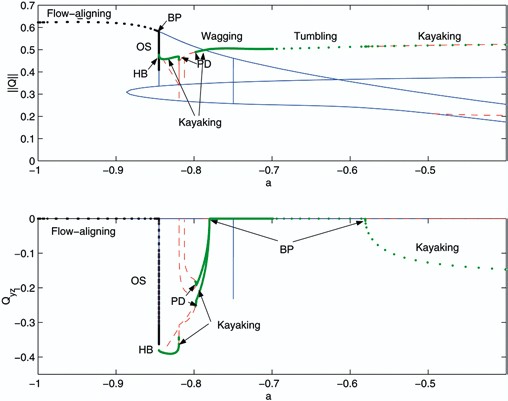

  

  "Virtual bifurcations" of the modified Doi model due to changes in the molecular aspect ratio parameter a, for fixed nematic concentration N=6 and fixed shear rate Pe=3.2. At large enough Pe and extreme aspect ratios $\left| a \right|$ ≈1, the only solution is the stable flow-aligning state; Fig. 7 illustrates this fact. Here we see a complex bifurcation from a single steady, flow-aligned state at large aspect ratios, to multiple steady/unsteady and in-plane/out-of-plane solution branches (OS denotes the out-of-plane steady state), all due to changes in molecular aspect ratio! Critical monodomain phase transitions at specific aspect ratios are predicted: flow-alignment-to-kayaking, kayaking-to-wagging, wagging-to-tumbling, tumbling-to-kayaking, and a period-doubling route to chaotic attractors in the discotic aspect ratio parameter range –0.8195<a<–0.7972

• The structure of the four lower, unstable branches of Figs. 7 and 8 is robust, corresponding to unstable, steady solutions arising in the weak shear limit from s _– and the isotropic state.

These remarks address the weak shear limit and the states that break nematic orientational degeneracy. Next we address the finite Pe-dependent continuation of these solution branches:

• The branch of stable K ₁ solutions persists until Pe≈2.923, clearly visible from the Q _yz projection in Fig. 8b. Pe≈2.923 is a saddle-node bifurcation, with the kayaking branch reversing back for lower Pe as an unstable K ₁ branch. This unstable periodic branch, as Pe is lowered, approaches in-plane motion, undergoing a period-halving bifurcation at Pe≈2.162, just as it connects to the previously unstable, in-plane T branch. This structure yields the second stable T/W state listed in Table 1 for 2.162<Pe <2.405, which is tumbling at the low end and wagging at the high end of these shear rates. Thus this interval has bi-stable attractors. Their respective domains of attraction are not addressed here.

• A stable W mode is depicted in Fig. 5, which we also use to illustrate the rod-discotic correspondence (Eq. 26). Note the significant order parameter oscillations (column 3), reflected in the shape distortions of the orientation ellipsoids (column 1). Such behavior is suppressed in an L-E description.

• At Pe≈2.405, the stable W mode bifurcates out-of-plane, creating a pair of stable, periodic K ₂ modes, one on either side of the shearing plane by virtue of the reflection symmetry (Eq. 28). One orbit is visualized in Fig. 4a for Pe=2.5. Note the significant order parameter oscillations, not captured by an L-E approximation. The energy of this attractor is equally shared between director and order parameter oscillations. From Table 1 we find tri-stability for a short band of shear rates, 2.405<Pe<2.536.

• At Pe≈2.536, a cascade of period doubling bifurcations of the double-K ₂ branch takes place over a very short range of Pe. The period-doubling sequence leads rapidly into a chaotic attractor.

• One also enters this chaotic range of Pe from higher shear rates by following the bifurcations of the unique FA branch as Pe drops below 4. At Pe≈3.717, a Hopf bifurcation of the steady FA branch leads to a stable, out-of-plane, periodic double-K ₂ branch. Figure 8a shows this as a single branch, while Fig. 8b shows both the max and min of Q _yz over a period. The symmetric mode tilted oppositely from the shearing plane has values –Q _yz, not shown here.

• The K ₂ branch persists for Pe<3.717 until approximately 3.29 when the first period doubling bifurcation occurs, giving way to a new branch of stable K ₂ solutions. As shown in Fig. 3b for Pe=3.27, each director executes a double loop in each period; the successive period-doublings yield four loops, then eight, etc.

• The period-doubled K ₂ monodomains tightly oscillate about the average director alignment, with visible shift of energy into the order parameters marked by shape distortions of the orientation ellipsoids. This behavior is not possible within L-E models.

• This bifurcation marks the onset of a period-doubling cascade to a chaotic attractor by Pe≈3.245. Figure 10 is a blow-up of four such period-doubling bifurcations. Just below Pe=3.245, all out-of-plane data converge to the chaotic attracting state. In-plane data cannot escape the shearing plane without an infinitesimal perturbation out-of-plane.

  Fig. 10.

  

  A blow-up of the sequence of period-doubling (PD) bifurcations indicated in Fig. 8 for the modified Doi model with constant diffusivity, N=6, aspect ratio r=${1 \over 3}$ , in the normalized shear rate range 3.2≤Pe≤ 3.3. The in-plane component Q _yy is used to illustrate the bifurcation structure, entering into the chaotic shear rate range from above. Here we show four PD bifurcations at Pe≈3.29, 3.253, 3.247, and 3.245. A PD cascade to chaotic motion occurs rapidly, prior to the value Pe=3.24, which requires a sequence of blowing-up operations to resolve

• Figure 4b visualizes the chaotic attractor for Pe=3.2 with significant director and order parameter variations. The motion consists of random jumping between the two fundamental kayaking modes, ${\bf K}_2^ +$ and ${\bf K}_2^ -$, which are weakly unstable. An explanation of this chaotic attractor in terms of a symbol sequence, where the symbols are defined by these two types of kayaking modes, seems plausible. An analytical description of this chaotic attractor presents a challenging dynamical systems problem.

• Table 1 summarizes the Modified Doi Model predictions of stable monodomains vs Pe: a unique attractor at low and sufficiently large shear rates, bi-stable and tri-stable periodic motions in a range of low shear rates, and a narrow window of weak shear rates with chaotic response.

The regime we call "chaotic" has to be substantiated by detailed statistics. We have confirmed irregular Poincare maps and positive Lyapunov exponents; e.g., an exponent of .005 is calculated for the Fig. 4b attractor. These diagnostics and bifurcation scenario are consistent with the rigorous statistical study of Grosso et al. [63], who computed the bifurcation diagram of the Smoluchowski partial differential equation of the Doi kinetic theory with infinite aspect ratio using AUTO97. It is remarkable that the finite-aspect-ratio quadratic closure model captures a similar chaotic bifurcation structure to the infinite-aspect-ratio kinetic theory, which compels further investigation.

Modified Doi Model with orientation-dependent rotary diffusivity and molecular aspect ratio 3 or EquationSource % MathType!MTEF!2!1!+- % feaaeaart1ev0aaatCvAUfKttLearuavP1wzZbqefuuDJXwAKbqedu % uDJXwAKbYu51MyVXgatuuDJXwAK1uy0HMmaeHbfv3ySLgzG0uy0Hgi % uD3Baebbfv3ySLgzGueE0jxyaibaieYlg9qrpeeu0dXdbba9q8qiW7 % rqaqFfpeea0de9pIe9arpK0dXdd9vspue9FjuP0-iq0lXdbba9pGe9 % qqFf0dXdbPYxe9vr0-vr0-LqpWqaaiaaciWacmaadaGabiaadaabau % aaaOqaamaalaaabaGaeGymaedabaGaeG4mamdaaaaa!3B42! ${1 \over 3}$

With orientation-dependent diffusivity, the flow-phase diagram (Fig. 11) of the modified Doi model simplifies considerably, altering some fundamental predictions regarding stable attractors (Table 2 ). Recall that our generalized Leslie criterion for steady vs unsteady selection in the weak flow limit was independent of rotary diffusivity (Eq. 21); note the number, mode type, and stability of monodomains for Pe≈0 are identical for both Modified Doi Models. In particular, the features robust to the choice at Eq. (21) are:

• The K ₁ monodomain is the unique attractor for low shear, disappearing through a saddle-node bifurcation at moderate shear rate.

• The unstable T branch at low Pe period-halves to create a stable T/W branch, overlapping for some range of Pe with the K ₁ attractor (a bi-stable region).

Fig. 11.

The flow-phase bifurcation diagram of the modified Doi model with orientation-dependent rotary diffusivity and discotic aspect ratio r=${1 \over 3}$ (or rod-like ratio 3). The nematic concentration is N=6; all transitions occur within the normalized shear range Pe⊂(0, 20). The weak-flow limit analysis, cf. Fig. 2, top left, is independent of diffusivity form, and the flow-selection criteria are identical to Fig. 8. The finite-flow bifurcations, however, are clearly modified. The fundamental feature is that the T/W branch avoids the sequence of bifurcations of Fig. 8, so that the out-of-plane transition to the K ₂ mode, and the subsequent cascade of PD bifurcations with a chaotic attractor, do not occur with orientation-dependent diffusivity in the Doi closure. A wagging to flow-alignment transition occurs for high Pe>20

Table 2. Stable solutions of the Modified Doi Model with orientational rotary diffusivity

However, several important changes due to orientation-dependent rotary diffusivity are predicted:

• The stable T/W branch persists for very high Pe, leading to a unique, unsteady, in-plane wagging monodomain at sufficiently high shear rates, vs a unique, steady flow-aligned state with constant diffusivity.

• Since the emergence of K ₂ bi-stable pairs and the period-doubling cascade to chaos for constant diffusivity arise from bifurcations of the T/W branch, that entire transition scenario is destroyed with Q-dependent diffusivity. Neither the K ₂ nor chaotic attractors are predicted.

Doi-Rey-Tsuji Model

Figure 12 depicts the bifurcation diagram of the Doi-Rey-Tsuji Model with constant rotary diffusivity and discotic aspect ratio ${1 \over 3}$ ; Table 3 describes the stable monodomains vs Pe. In the text surrounding Fig. 2 we explained how the weak flow limit, Pe≈0, yields the same selection criteria of steady and unsteady states from the nematic equilibria s ₊,s _–,0 for the Doi and Rey-Tsuji closures. Comparison of Figs. 8 and 12 shows even stronger agreement, indeed almost identical transition phenomena except for the small chaotic band which this closure does not capture:

• All seven solution branches that emerge for Pe≈0 match, in type and stability!

• The unique stable attractor in the start-up of shear is a K ₁ orbit.

• The low shear, unstable T branch undergoes a period-halving bifurcation into a stable T/W branch, yielding bi-stability with the K ₁ monodomain.

• The stable T/W branch bifurcates out-of-plane, creating a pair of stable K ₂ modes, and a shear-rate interval of tri-stability.

• The stable K ₁ branch loses stability in a saddle-node bifurcation at intermediate shear rates, never to emerge again.

• The high shear-rate attractor is the steady, in-plane FA state.

Fig. 12.

The flow-phase bifurcation diagram for the Rey-Tsuji model with constant diffusivity, nematic concentration N=6, and discotic aspect ratio r=${1 \over 3}$ , or a=–0.8. The flow-induced transitions occur within the normalized shear range Pe⊂(0, 10). As noted from Fig. 2, top right together with our analysis of the unsteady selection criteria, the same seven states emerge for the Rey-Tsuji and Doi closures at this aspect ratio. For finite shear rates, the difference between closures lies in the bifurcations of the double branch of K ₂ kayaking modes, each tilted to one side of the shearing plane. In the Rey-Tsuji model, these branches are born in the same way through an out-of-plane instability of a stable wagging mode, but do not undergo a PD cascade to chaos; rather they simply persist until a so-called torus bifurcation (denoted TR by the software XPPAUT) and transition to the stable flow-aligning, in-plane state at Pe≈3.375. The tumbling to wagging transition takes place roughly at Pe=1.796, so the stable interval of this branch always consists of wagging motion

Table 3. Stable solutions of the Doi-Rey-Tsuji Model with constant rotary diffusivity and discotic aspect ratio r=$\frac {1} {3}$

The noteworthy qualitative difference between the Modified Doi and Doi-Rey-Tsuji Models centers upon how the K ₂ symmetric pairs bifurcate and lose stability, which is an extremely subtle phenomenon, yet predicted in both models to occur over approximately one dimensionless shear-rate unit.

Doi-Rey-Tsuji Model with orientational diffusivity, discotic aspect ratio EquationSource % MathType!MTEF!2!1!+- % feaaeaart1ev0aaatCvAUfKttLearuavP1wzZbqefuuDJXwAKbqedu % uDJXwAKbYu51MyVXgatuuDJXwAK1uy0HMmaeHbfv3ySLgzG0uy0Hgi % uD3Baebbfv3ySLgzGueE0jxyaibaieYlg9qrpeeu0dXdbba9q8qiW7 % rqaqFfpeea0de9pIe9arpK0dXdd9vspue9FjuP0-iq0lXdbba9pGe9 % qqFf0dXdbPYxe9vr0-vr0-LqpWqaaiaaciWacmaadaGabiaadaabau % aaaOqaamaalaaabaGaeGymaedabaGaeG4mamdaaaaa!3B42! ${1 \over 3}$

The flow-phase diagram (Fig. 13) and stable attractors (Table 4 ) are qualitatively similar to the Modified Doi Model (Fig. 11, Table 2 ) with orientational diffusivity and the same aspect ratio. The only meaningful differences are quantitative, and the transition scenarios are remarkably consistent: a unique K ₁ attractor in start-up, bi-stable with a T/W mode for some intermediate shear rates, then a unique stable T/W attractor in the high shear range.

Fig. 13.

The flow-phase bifurcation diagram for the Doi-Rey-Tsuji model with orientation-dependent rotary diffusivity, N=6, a=–0.8. The bifurcations are similar to those of previous diagrams. Two primary stable branches emerge over this range of Pe, overlapping for an interval of Pe leading to bi-stable attractors. The tumbling-wagging transition takes place at Pe=5.834

Table 4. Stable monodomains of the Doi-Rey-Tsuji Model with orientational

The above four models were analyzed in two excellent papers by Singh and Rey [128], who worked at the same fixed aspect ratio (a=–0.8) and fixed polymer concentration (N=6) to study sheared discotic nematic liquids. Our simulations generalize theirs by illustrating transitions due to variable aspect ratio, and by a more detailed resolution of the bifurcation diagrams captured by the software package XPPAUT of Ermentrout [42]. One consequence of our studies on the Doi and Rey-Tsuji closures, with or without orientational rotary diffusivity, is that the logrolling steady states exist but are always unstable. Even so, Larson and Ottinger found stable logrolling states in simulations of the Doi kinetic theory for infinite aspect ratio rods [86], which have been subsequently confirmed in detailed kinetic simulations by [43, 54, 55, 93, 96]. As shown in Fig. 2 and the tensor selection criteria, the Hinch-Leal closures [69, 70, 71] preferentially select stable LR states in the weak shear limit, for all aspect ratios. We turn to their predictions for finite aspect ratio fluids.

Modified Doi-HL1 Model

Figure 14 and Table 5 depict the bifurcation diagram and stable monodomains for shape parameter value $\left| a \right| = {{24} \over {26}}$ , corresponding to molecular aspect ratio r=5 or ${1 \over 5}$ . The key features are:

• The LR state is the unique attractor at start-up of shear.

• The unstable T state stabilizes in a period-halving bifurcation, leading to bi-stable regimes for a range of Pe, first with LR then K ₁ monodomains.

• The LR state bifurcates to a K ₁ attractor in the most intuitively natural, steady-unsteady transition (Hopf bifurcation): the major director first aligns then oscillates about the vorticity axis as the shear rate increases.

• The K ₁ state is lost through a saddle-node bifurcation at an intermediate shear rate, and the unstable branch doubles back at lower shear to connect with the T branch precisely at the period-halving, stability transition.

• The observable attractors from Table 5 are, in terms of increasing shear rate, a unique LR state, then bi-stable LR and T states, then bi-stable T and K ₁ states, then a unique T/W branch of monodomains for high Pe.

• The monodomain response is predicted to be steady at low shear, bi-stable steady and in-plane tumbling for a very narrow window of shear rates, then bi-stable transient states (one in-plane, another out-of-plane), and finally in-plane unsteady attractors at sufficiently high shear rates.

Fig. 14.

The bifurcation diagram for the Doi-HL1 model with constant rotary diffusivity, N=6, and shape parameter $a = - {{24} \over {26}}$ corresponding to discotic aspect ratio r=${1 \over 5}$ . As explained in Fig. 2, lower left and surrounding text, this closure selects a unique, stable LR steady state in weak shear. This stable branch persists until a Hopf bifurcation at Pe≈8.638 creates a stable K ₁ kayaking branch, in which the major director now rotates around the vorticity axis. The stable kayaking branch persists until a saddle-node bifurcation at Pe≈15.85. (A physically inconsequential bifurcation occurs for Pe between 5 and 6, leading to unstable kayaking solutions.) The unstable T solution arising from s ₊ in weak shear stabilizes at Pe≈7.509 through a PD bifurcation, remaining stable beyond Pe=20. The stable attractors are summarized in Table 5

Table 5. Stable solutions of the Modified Doi-HL1 model with constant rotary diffusivity

Modified Doi-HL1 Model with orientational rotary diffusivity

As detailed in Table 6 , the incorporation of orientation-dependent rotary diffusivity for the HL1 closure scheme has no qualitative effect on the results for aspect ratios 5 and ${1 \over 5}$ . The quantitative effect is to shift all bifurcations to higher shear rates, so that the LR attractor is predicted to be the unique response until Pe≈22, and the bi-stable region lasts for a span of 48 in Pe. The basic bifurcation structure, however, is remarkably robust at this aspect ratio.

Table 6. Stable monodomains: Doi-HL1 Model with orientational rotary diffusivity

Modified Doi-HL2 Models for either rotary diffusivity

The Modified Doi-HL2 Model is also robust to constant or orientation-dependent rotary diffusivity. The flow-phase diagram for constant diffusivity is given in Fig. 15; Tables 7 and 8 indicate all stable monodomains vs Pe. We choose aspect ratio 5 to compare the HL2 and HL1 closures.

Fig. 15.

The bifurcation diagram for the Doi-HL2 model. The parameter values are N=6, $a = - {{24} \over {26}}$ . The logrolling steady state exists for all values of Pe and is stable. Tumbling/wagging stable solutions exist at low and high shear rates, first losing stability in a PD bifurcation at Pe=2.034, then regaining stability in another PD bifurcation at Pe=8.179

Table 7. Stable solutions of the Modified Doi-HL2 model with constant diffusivity

Table 8. Stable monodomains: Doi-HL2 Model with orientational diffusivity

The key features of the HL2 models are:

• The LR state is stable for all Pe!

• The in-plane T mode is stable at the start-up of shear, loses stability in an intermediate window of shear rates, then regains stability for all sufficiently high shear rates. The T-to-W transition, as always, occurs at some intermediate shear rate.

• At low and sufficiently high shear rates, bi-stable LR and T/W states prevail; the internal window has only the LR attractor.

• The HL2 closure is seen to suppress stable kayaking monodomains, and indeed no unsteady out-of-plane motion is stable.

Conclusion

The role of finite-aspect-ratio effects in monodomain response to simple shear, and to more general linear flows, has been studied from various tensor orientation models. Several symmetry properties were developed for mesoscopic Doi-type models, independent of closure approximation. These properties were used to develop intuition about finite-aspect-ratio nematic liquids in shear and related linear flows, and to extrapolate theoretical and experimental results from rods to discotics, and from finite aspect ratio fluids to extremely large aspect ratio fluids. Symmetries of a fixed aspect ratio fluid in simple shear were further used to explain necessary constraints on monodomain motion. E.g., a monodomain that tilts out-of-plane cannot return to in-plane orientation in finite time; all such motion has a mirror-reflection in the opposite direction out of the shearing plane, which leads to bi-stable kayaking modes whose major director oscillates between the vorticity axis and shearing plane. It will be interesting to explore whether such bi-stable attractors exist in laboratory experiments with model monodisperse nematic liquids; indeed, some closure schemes predict these attractors and others do not. All solutions and monodomain transitions vs shear rate and aspect ratio have been compared with Leslie-Ericksen model behavior; clearly, the tensor theories capture new properties and new phenomena which require validation both from kinetic theory and experiment. This will necessitate computation of the rheological predictions associated with the tables given here of all stable monodomains and their shear-rate and aspect-ratio transitions, which we report elsewhere [52].

By exploring four different closure schemes, with and without orientational rotary diffusivity, we have shown that with finite-aspect-ratio effects, the Doi mesoscopic theory captures a diversity of monodomain features at fixed, high (nematic) concentrations:

• Weak-shear, monodomain selection mechanisms include features that are robust to closure rule and molecular aspect ratio: the multiplicity and "taxonomy" of possible monodomain modes (steady and unsteady) varies only slightly and in a computable fashion; reflection-symmetry with respect to the shearing plane insures out-of-plane steady and so-called K ₂ kayaking periodic modes always occur in pairs.

• Other selection criteria are highly sensitive to closure scheme and molecular aspect ratio: which of the multiple states are stable and unstable, steady and unsteady, in-plane vs vorticity-aligned or out-of-plane. One can easily change models and infer unique, bi-stable, or tri-stable attracting monodomain modes, with quite different orientational properties, at the same shear rate and nematic concentration.

• Shear-rate-dependent transition scenarios likewise are strongly sensitive to closure scheme and molecular aspect ratio.

Many, but each intuitively plausible, scenarios are detailed. This diversity of mesoscopic behavior is consistent with an interpretation that a "monodisperse finite-aspect-ratio fluid" and second-moment closure scheme play the role of broad-brush fitting parameters for laboratory nematic fluids. Macromolecular fluids always violate assumptions of current theory; real fluids are polydisperse with statistical aspect-ratio distributions, and all but the most pristine laboratory samples consist of many monodomains separated by transitional regions associated with defects. The Maier-Saupe potential employed here assumes a single parameter (N), short-range potential, which we have fixed in this study and suppressed its dependence on aspect ratio. Even given these shortcomings, the diversity of model behavior predicted in this paper reflects much of the diversity of bulk experimental behavior of nematic polymers vs shear rate. We suppose that in restricted flow regimes one can accurately accomplish model fitting to monodomain states and nontrivial transition phenomena within this class of models. From a reasonable fit between experimental monodomain response and model predictions, one can then confidently proceed to model the onset of mesoscopic structure formation. Various transient monodomain states documented here are corroborated by full kinetic simulations [43, 54, 55, 63], including regions of nematic concentration and shear rate with highly erratic bulk motion. If these monodomain attractors are confirmed in the laboratory, as many have already, then their diversity implies very different routes to subsequent mesostructure formation and flow instabilities, a topic which we are currently exploring [56] with the current study as a guide.

Appendix. Viscosity coefficients

The results of Jeffery [74], Batchelor [9] as well as Hinch and Leal [69, 70] on ellipsoidal suspensions in a viscous solvent are utilized in the derivation of the viscous stress [140]:

$$\matrix{ {\eta _s = \eta + 3/2\nu kT\zeta _3 ,} \hfill \cr {\zeta _3 = {{\zeta ^{\left( 0 \right)} } \over {I_1 }},\;\;\zeta _1 = \zeta ^{\left( 0 \right)} \left( {{1 \over {I_3 }} - {1 \over {I_1 }}} \right),\;\;\zeta _2 = \zeta ^{\left( 0 \right)} \left[ {{{J_{\rm I} } \over {I_1 J_3 }} + {1 \over {I_1 }} - {2 \over {I_3 }}} \right],} \hfill \cr {I_1 = 2r\int_0^ \propto {{{dx} \over {\sqrt {\left( {r^2 + x} \right)\left( {1 + x} \right)^3 } }},\;\;I_3 = r\left( {r^2 + 1} \right)\int_0^\infty {{{dx} \over {\sqrt {\left( {r^2 + x} \right)\left( {1 + x} \right)^2 \left( {r^2 + x} \right)} }}} ,} } \hfill \cr {J_1 = r\int_0^\infty {{{xdx} \over {\sqrt {\left( {r^2 + x} \right)\left( {1 + x} \right)^3 } }},\;\;J_3 = r\int_0^\infty {{{xdx} \over {\sqrt {\left( {r^2 + x} \right)\left( {1 + x} \right)^2 \left( {r^2 + x} \right)} }}.} } } \hfill \cr } $$

(A1)

References

Alderman NJ, Mackley MR (1985) Mol Cryst Liq Cryst 79:149
Andrews NC, Edwards BJ, McHugh AJ (1995) J Rheol 39:1161
Andrews NC, Edwards BJ, McHugh AJ (1996) J Rheol 40(3):459
Archer L, Larson RG (1995) J Chem Phys 103:3108
Atkin RJ (1970) Arch Ration Mech Anal 38:224
Baek SG, Magda JJ, Larson RG (1993) J Rheol 37:1201
Baek SG, Magda JJ, Larson RG (1994) J Rheol 38:1473
Bandyopadhyay R, Basappa G, Sood AK (2000) Phys Rev Lett 84(9):2022
Batchelor GK (1970) J Fluid Mech 41(3):545
Beris AN, Edwards BJ (1994) Thermodynamics of flowing systems with internal microstructure. Oxford Science Publications
Berry GC (1988) Mol Cryst Liq Cryst 165:333
Berry GC (1991) J Rheol 35:943
Berry GC, Tan Z (2001) Rheological and rheo-optical studies of shear deformation on nematic solutions of poly(1,2-PET). Preprint. Univ of Pittsburgh
Bhave AV, Menon RK, Armstrong RC, Brown RA (1993) J Rheol 37:413
Bird B, Armstrong RC, Hassager O (1987) Dynamics of polymeric liquids, vols 1 and 2. Wiley
Boudreau DM, Winter HH, Lillya CP, Stein RS (1999) Rheol Acta 38:503
Bruinsma R, Safinya CR (1991) Phys Rev A 43:5377
Burghardt WR (1998) Macromol Chem Phys 199:471
Burghardt WR, Fuller GG (1990) J Rheol 34:959
Burghardt WR, Fuller GG (1991) Macromolecules 24:2546
Carlsson T (1987) Mol Cryst Liq Cryst 104:307
Carlsson T, Skarp K (1986) Liq Cryst 1:455
Chandrasekhar S (1992) Liquid crystals, 2nd edn. Cambridge University Press
Chaubal CV, Leal LG, Fredrickson GH (1995) J Rheol 39:73
Chillingworth DRJ, Vicente Alonso E, Wheeler AA (2001) J Phys A Math Gen 34:1393
Cladis PE, Torza S (1975) Phys Rev Lett 35:1283
Clar MG, Saunders FC, Shanks IA, Leslie FM (1981) Mol Cryst Liq Cryst 70:195
Cocchini F, Aratari C, Marrucci G (1990) Macromolecules 23:4446
de Gennes P-G (1971) Mol Cryst Liq Cryst 12:193
de Gennes P-G, Prost A (1993) The physics of liquid crystals, 2nd edn. Oxford University Press
Doedel EJ et al. (1995) AUTO95: continuation and bifurcation software for ordinary differential equations. Concordia University
Doedel EJ et al. (1997) AUTO97: continuation and bifurcation software for ordinary differential equations. Concordia University
Doi M (1981) J Polym Sci Polym Phys Ed 19:229
Doi M, Edwards SF (1986) The theory of polymer dynamics. Oxford University Press (Clarendon), London-New York
Donald AM, Windle AH (1992) Liquid crystalline polymers. Cambridge Solid State Science Series, Cambridge University Press
Dupré DB (1982) Techniques for the evaluation of material constants in lyotropic systems and the study of pretransitional phenomena in polymer liquid crystals. In: Ciferi A, Krigbaum W, Meyer RB (eds) Polymer liquid crystals. Academic Press, New York, chap 7
Edie D, McHugh JJ (1996) Carbon 34(11):1315
Edwards BJ, Pilitsis S, Beris AN (1988) Proceedings of the Xth International Congress on Rheology, vol 1, p 312
Edwards BJ (1991) The dynamical continuum theory of liquid crystals. PhD thesis, Univ of Delaware
Ericksen JL (1960) Arch Ration Mech Anal 4:231
Ericksen JL (1962) Arch Ration Mech Anal 9:371
Ermentrout B (2001) XPPAUT-the differential equation tool. University of Pittsburg
Faraoni V, Maffetone PL (1999) J Rheol 43:829
Farhoudi Y, Rey AD (1993) J Rheol 37:289
Feng J, Chaubal CV, Leal LG (1998) J Rheol 42:1095
Feng J, Sgalari G, Leal LG (2000) J Rheol 44:1085
Feng J, Tao J, Leal LG (2001) Roll cells and disclinations in sheared nematic polymers. Preprint
Forest MG, Wang Q, Zhou H (2000) Phys Fluids 12(3):490
Forest MG, Wang Q, Zhou H (2000) Phys Rev E 61(6):6655
Forest MG, Wang Q, Zhou H (2001) Liq Cryst 28(5):717
Forest MG, Wang Q, Zhou H (2001) Physica D 152/153:288
Forest MG, Wang Q (2002) Rheological predictions of Doi moment-closure models for finite-aspect-ratio nematic polymers (in preparation)
Forest MG, Wang Q, Zhou R (2002) Symmetries of the Doi kinetic theory for nematic polymers of arbitrary aspect ratio: at rest and in linear flows. Submitted to Phys Rev E, February, 2002, and UNC-CH Program in Applied Mathematics Preprint PAMPS-2002–08 (2002)
Forest MG, Wang Q, Zhou R (2002) The weak shear limit of the isotropic-nematic phase diagram for nematic polymers from Doi molecular theory. UNC-CH Program in Applied Mathematics Preprint PAMPS-2002–16
Forest MG, Wang Q, Zhou R (2002) The monodomain phase diagram for sheared nematic polymers from Doi molecular theory. UNC-CH Program in Applied Mathematics Preprint PAMPS-2002–17
Forest MG, Wang Q, Zhou H (2002) Flow-orientation structure evolution of tumbling and kayaking nematic polymers in the gap between shearing plates. UNC-CH Program in Applied Mathematics Preprint Series PAMPS-2002–04
Forest MG, Wang Q, Zhou R (2002) Exact director torque dynamics of nematic polymers from Doi molecular theory and mesoscopic upscaling approximations. UNC-CH Program in Applied Mathematics Preprint Series PAMPS-2002–18
Fuller GG (1995) Optical rheometry of complex fluids. Oxford University Press, Oxford
Gahwiller C (1972) Phys Rev Lett 28:1554
Golubitsky M, Chillingworth D (2001) University of Houston (preprint)
Gotsis AD, Baird DG (1986) Rheol Acta 25:275
Grizzuti N, Cavella S, Cicarelli P (1990) J Rheol 34:1293
Grosso M, Keunings R, Crescitelli S, Maffettone PL (2001) Prediction of chaotic dynamics in sheared liquid crystalline polymers. Preprint (2001) and lecture, Society of Rheology Annual Meeting, Hilton Head, SC, February
Han CD, Kim SS (1994) J Rheol 38:13
Han WH, Rey AD (1994) Phys Rev E 50:1688
Han WH, Rey AD (1994) J Rheol 38:1317
Hand GL (1962) J Fluid Mech 13:33
Hess S (1976) Z Naturforsch Teil 31A:1034
Hinch EJ, Leal LG (1972) J Fluid Mech 52(4):683
Hinch EJ, Leal LG (1973) J Fluid Mech 57(4):753
Hinch EJ, Leal LG (1976) J Fluid Mech 76(1):187
Hongladarom K, Burghardt W (1993) Macromolecules 26:785
Hongladarom K, Burghardt W, Baek SG, Cementwala S, Magda JJ (1993) Macromolecules 26:772
Jeffery GB (1922) Proc Roy Soc London Ser A 102:161
Jenkins JT (1978) Ann Rev Fluid Mech 10:197
Kaiser P, Wiese W, Hess S (1992) J Non-Equilib Thermodyn 17:153
Kevrekides Y, Theodoropoulos K, Qian Y-H (2000) Proc Natl Acad Sci 97:9840
Kiss G, Porter RS (1978) J Polym Sci Polym Symp 65:193
Kiss G, Porter RS (1980) J Polym Sci Polym Phys Ed 18:361
Kroger M, Sellers HS (1995) J Chem Phys 103:807
Kupferman R, Kawaguchi M, Denn MM (2000) J Non-Newtonian Fluid Mech 91:255
Kuzuu N, Doi M (1983) J Phys Soc Japan 52:3486
Kuzuu N, Doi M (1984) J Phys Soc Japan 53:1031
Larson RG, Mead DW (1989) J Rheol 33:1251
Larson RG (1990) Macromolecules 23:3983
Larson RG, Ottinger H (1991) Macromolecules 24:6270
Larson RG, Mead DW (1992) Liq Cryst 12:751
Larson RG, Mead DW (1993) Liq Cryst 15:151
Larson RG (1998) Rheology of complex fluids. Oxford University Press
Leslie FM (1968) Arch Ration Mech Anal 28:265
Leslie FM (1979) In: Brown HG (ed) Advances in liquid crystals. Academic Press, p 4
Maffetone PL (1992) J Non-Newtonian Fluid Mech 45:339
Maffettone PL, Crescitelli S (1994) J Rheol 38:1559
Maffettone PL, Marrucci G (1991) J Non-Newtonian Fluid Mech 38:273
Maffettone PL, Marrucci G, Mortier M, Moldenaers P, Mewis J (1994) J Chem Phys 100:7736
Maffettone PL, Crescitelli S (1995) J Non-Newtonian Fluid Mech 59:73
Maffettone PL, Sonnet AM, Virga EG (2000) J Non-Newtonian Fluid Mech 90:283
Magda JJ, Baek S-G, de Vries L, Larson RG (1991) Macromolecules 24:4460
Manneville P (1981) Mol Cryst Liq Cryst 70:223
Marrucci G, Maffetone PL (1989) Macromolecules 22:4076
Marrucci G, Maffetone PL (1990) J Rheol 34:1217, 1231
Marrucci G (1991) Macromolecules 24:4176
Marrucci G, Greco F (1991) Mol Cryst Liq Cryst 206:17
Marrucci G, Greco F (1992) J Non-Newtonian Fluid Mech 44:1
Marrucci G, Greco F (1993) Adv Chem Phys 86:331
Mather PT, Pearson DS, Burghardt WR (1995) J Rheol 39:627
Mather PT, Pearson DS, Larson RG (1996) Liq Cryst 20(5):527
Mather PT, Pearson DS, Larson RG (1996) Liq Cryst 20(5):539
Mather PT, Romo-Uribe A, Han CD, Kim SS (1997) Macromolecules 30:7977
Meiboom S, Hewitt RC (1973) Phys Rev E 30:261
Mewis J, Moriter M, Vermant J, Moldenaers P (1997) Macromolecules 30:1323
Moldenaers P, Mewis J (1986) J Rheol 30:567
Moldenaers P (1987) PhD Thesis, Katholiecke Universiteit Leuven
Moldenaers P, Fuller G, Mewis J (1989) Macromolecules 22:960
Muller JA, Stein RS, Winter HH (1994) Rheol Acta 33:473
Muller JA, Stein RS, Winter HH (1996) Rheol Acta 35:160
Navard P (1986) J Polym Sci Polym Phys Ed 24:435
Olmsted PD, Goldbart PM (1990) Phys Rev A 41:4578
Olmsted PD, Goldbart PM (1992) Phys Rev A 46:4966
Olmsted PD, Lu C (1997) Phys Rev E 56:55
Pieranski P, Guyon E (1974) Phys Rev Lett 32:924
Pradadarao M, Pearce EM, Han CD (1982) J Appl Polym Sci 27:1343
Rey AD (1995) Macromol Theory Simul 4(5):857
Rienacker G, Hess S (1999) Physica A 267:294
See H, Doi M, Larson RG (1990) J Chem Phys 92(1):792
Semenov AN (1983) Sov Phys JETP 85:321
Semenov AN (1986) Sov Phys JETP 66:712
Singh AP, Rey AD (1998) Rheol Acta 37:30, 374
Skarp K, Carlsson T, Lagerwall T, Stebler B (1981) Mol Cryst Liq Cryst 66:199
Srinivasarao M, Berry GC (1991) J Rheol 35:379
Srinivasarao M, Garay RO, Winter HH, Stein RS (1992) Mol Cryst Liq Cryst 223:29
Tseng HC, Silver DL, Finlayson BA (1972) Phys Fluids 15:1213
Tsuji T, Rey AD (1997) J Non-Newtonian Fluid Mech 73:127
Van Horn BL, Winter HH (2000) Rheol Acta 39:294
Vicente Alonso E, Wheeler AA, Sluckin TJ (2002) Nonlinear dynamics of a nematic liquid crystal in the presence of a shear flow. Preprint. Univ of Southampton
Volovik GE (1980) JETP Lett 31:273
Wang L, Rey AD (1997) Liq Cryst 23(1):93
Wang Q (1997) J Rheol 41(5):943
Wang Q (1997) J Non-Newtonian Fluid Mech 72:141
Wang Q (2002) J Chem Phys 116(20):9120
Wissbrun K (1993) J Rheol 37:777
Yan NX, Labes MM, Baek SG, Magda JJ (1994) Macromolecules 27:2784
Yang IK, Shine AD (1992) J Rheol 36:1079
Zhou W-J, Kornfield JA, Burghardt WR (2001) Macromolecules 34:3654
Zhou W-J, Kornfield JA, Ugaz V, Burghardt WR, Link D, Clark NA (1999) Macromolecules 31:8474
Zuniga I, Leslie FM (1989) Liq Cryst 5:725
Acknowledgment and disclaimer.
Effort sponsored by the Air Force Office of Scientific Research, Air Force Materials Command, USAF, under grant numbers F49620-99-1-0003 and F49620-00-1-0008. The US Government is authorized to reproduce and distribute reprints for governmental purposes notwithstanding any copyright notation thereon. The views and conclusions contained herein are those of the authors and should not be interpreted as necessarily representing the official policies or endorsements, either expressed or implied, of the Air Force Office of Scientific Research or the US Government.
Author information
Authors and Affiliations
Corresponding author