
Abstract
For each noninteger complex number λ, the Hilbert matrix
defines a bounded linear operator on the Hardy spaces \(\mathcal{H}^{p}\), 1<p<∞, and on the Korenblum spaces \(\mathcal{A}^{-\tau}\), τ>0. In this work, we determine the point spectrum with multiplicities of the Hilbert matrix acting on these spaces. This extends to complex λ results by Hill and Rosenblum for real λ. We also provide a closed formula for the eigenfunctions. They are in fact closely related to the associated Legendre functions of the first kind. The results will be achieved through the analysis of certain differential operators in the commutator of the Hilbert matrix.
1 Introduction
For each λ∈ℂ∖ℤ, the Hilbert matrix of parameter λ is
Hill [4], see also the work by Rosenblum [9], showed that any nonnegative complex number is a latent root of H λ . He also determined the multiplicities of all latent roots of H λ for nonnegative real λ and in particular for all positive integers, thus solving the eigenvalue problem for λ real. The aim of this work is to extend this result to λ∈ℂ∖ℝ. Indeed, if we restrict ourselves to the Hardy space or the Korenblum classes, then the eigenvalue problem is completely solved for complex λ. We will also provide an explicit formula for the eigenfunctions of H λ and identify them with the associated Legendre functions of the first kind.
In Sect. 2, we will review some known integral representations of the Hilbert matrix based on the Hankel form. We will also show that the Hilbert matrix preserves the Hardy spaces and the Korenblum spaces. The fact that H λ acts boundedly on \(\mathcal{H}^{p}\), 1<p<∞, has already been proved in [2] for λ=1.
In Sect. 3, we will show that H λ almost commutes with certain differential operators D. Indeed, we are interested in the operator defined formally by
where D is a differential operator.
Finally, in Sect. 4, we will provide a description of the point spectrum of the Hilbert matrix H λ acting on the Hardy spaces \(\mathcal{H}^{p}\), for p>1, and on the Korenblum spaces \(\mathcal{A}^{-\tau}, \mathcal{A}_{0}^{-\tau}\), for 0<τ<1.
2 Integral Operator Representations
Let \(\mathbb{D}\) denote the unit disk. For each 1≤p<∞, the Hardy space \(\mathcal{H}^{p} \) consists of those functions f analytic on \(\mathbb{D}\) for which the norm
is finite. We also denote by \(\mathcal{H}^{\infty}\) the space of bounded analytic functions on \(\mathbb{D}\) endowed with the supremum norm.
In addition, we will also consider the Korenblum spaces, which are special cases of weighted spaces of analytic functions. For each real number τ>0, the Banach space \(\mathcal{A}^{-\tau}\) consists of those functions f analytic on \(\mathbb{D}\) for which the norm
is finite. The Banach subspace \(\mathcal{A}_{0}^{-\tau}\) consists of those f in \(\mathcal{A}^{-\tau}\) for which
The Hilbert matrix of parameter λ can be represented with the help of the Hankel form with symbol t λ/κ, where κ=e 2πiλ−1 and λ∈ℂ∖ℤ. More precisely, from the identity
we see that the Hilbert matrix of parameter λ extends to a bounded operator on the Hardy space \(\mathcal{H}^{2}\), which will also be denoted by H λ , defined by
Obviously, it is also possible to define H λ f for f in the Hardy space \(\mathcal{H}^{1}\). However, this representation is not easy to work with. Therefore, we shall use alternative integral representations obtained by changing the path of integration in the above formula. The more classical representation for the case \(f\in \mathcal{H}^{1}\) and ℜλ>0 is obtained in the following way: the Hilbert matrix of parameter λ is
Thus for \(f(z)=\sum_{n=0}^{\infty}a_{n}z^{n} \in \mathcal{H}^{1}\), Hardy’s inequality (see [3], for instance) implies that
Hence the power series
has bounded coefficients, thus its radius of convergence is greater than or equal to 1 and we obtain a well-defined analytic function H λ f on the disc \(\mathbb{D}\) for each \(f\in\mathcal{H}^{1}\). A standard computation shows that, for ℜλ>0, we have
Indeed, if we set
then

Therefore,
A similar argument yields that the same representation holds true when f is in the Korenblum space \(\mathcal{A}^{-\tau},\; 0<\tau<1\). For the remaining case ℜλ≤0, we shall use a similar approach. We will integrate along the boundary of a Stolz angle at 1. Throughout the rest of this work, C will be the closed path defined by the boundary of the Stolz angle \(\{z\in\mathbb{D}: \vert1-z \vert\leq \sigma(1-\vert z\vert) \}\) where σ>1 is fixed. We assume that C is positively oriented, that is, in the counterclockwise sense. Now, for 0<ε<1, we see that the straight line with equation ℜz=ε and C meet exactly at two conjugate points a ε and \(\overline{a_{\varepsilon}}\), where ℑa ε >0. To fix notation, for any nonnegative intergers n and m, we set z n+m+λ−1=e (n+m+λ−1)logz, where logz=ln|z|+iargz with argz∈[0,2π); of course, other definitions are possible in the argument below. Let C ε denote the subarc of C that goes from a ε to \(\overline{a_{\varepsilon}}\) in the counterclockwise sense. Next, consider the closed contour \(C^{\prime}_{\varepsilon}\) obtained by adding the line segments ℑz=±ℑa ε and a semicircle (on the left half-plane) of center 0 and radius ℑa ε to C ε . With f in \(\mathcal{H}^{1}\) or \(\mathcal{A}^{-\tau}\), using Cauchy’s theorem, we have
Thus, making ε tend to 0, one easily sees that the following integral representation holds:
Now, (2.1) makes sense also for ℜλ≤0, which provides an integral representation for H λ whenever \(\lambda\in\Bbb{C} \setminus\Bbb{Z}\). Moreover, as the above argument shows, this representation is independent of the aperture σ of the Stolz angle.
Theorem 2.1
Let f be analytic on \(\mathbb{D}\) and integrable on [0,1], and let H λ f be as in (2.1). Then
-
(i)
if f∈L p([0,1]), 1<p<∞, then \(H_{\lambda }f\in\mathcal{H}^{p}\);
-
(ii)
if 0<τ<1 and |f(x)|=O((1−x)−τ) as x→1, then \(H_{\lambda}f\in\mathcal{A}^{-\tau}\);
-
(iii)
if 0<τ<1 and |f(x)|=o((1−x)−τ) as x→1, then \(H_{\lambda}f\in \mathcal{A}_{0}^{-\tau}\).
In particular, if X is one of the spaces \(\mathcal{H}^{p}\), 1<p<∞, \(\mathcal{A}^{-\tau}\) or \(\mathcal{A}_{0}^{-\tau}\), 0<τ<1, then H λ is a bounded linear operator from X into itself. Moreover, H λ is the unique operator T on X such that
where by abuse of notation we write z for the identity function on \(\mathbb{D}\).
Proof
To prove (i), observe that if \(h\in\mathcal{H}^{q}\), with 1/p+1/q=1, a straightforward computation shows that
Since the arc length measure on C is a Carleson measure, by Hölder’s inequality, we find that
where M is a positive constant independent of f and h. By duality, this implies
To prove (ii), observe that if |f(x)|≤M(1−x)−τ, where M is a positive constant and 0<τ<1, then

for all \(z\in\mathbb{D}\). It is easy to see that the last term in the above display is uniformly bounded in \(z\in\mathbb{D}\), which shows that \(H_{\lambda}f\in\mathcal{A}^{-\tau}\).
To prove (iii), observe first that
Hence, the previous estimate yields that
for a positive constant M 1>0 and for any 0<δ<1. Now, the boundedness of H λ on the spaces considered in the statement of the theorem follows immediately from the closed graph theorem. Finally, the fact that
is obvious, since
The uniqueness assertion follows immediately from the fact that polynomials are dense in \(\mathcal{H}^{p}\), 1<p<∞, and \(\mathcal{A}_{0}^{-\tau}, 0<\tau<1\) and weak-star dense in \(\mathcal{A}^{-\tau}\). □
Remark
The case in which \(X=\mathcal{H}^{p}\), 1<p<∞, and λ=1 was proved earlier in [2].
3 Differential Operators in the Commutator
The purpose of this section is to prove that H λ almost commutes with certain differential operators D. Indeed, we are interested in the operator defined formally by
We shall only investigate linear differential operators of second order with polynomial coefficients. These are defined by
where
The main result of this section provides a class of such operators where the commutator in question has rank one. We shall assume throughout that \(\lambda\in\mathbb{C\setminus Z}\).
Theorem 3.1
Let D be a differential operator as in (3.2). Assume that the polynomials q 1,q 2,q 3 in (3.2) satisfy

for some constants α,γ∈ℂ. Then for every \(f\in\mathcal{A}^{-\tau}\), 0<τ<1, we have
where C is the contour in (2.1).
Proof
By means of the integral representation formula (2.1), we see that
Observe that Df∈L 1(C) whenever f∈A −τ so that the integrals involved make sense. Now write z=ζ−1, for |ζ|>1, and for a polynomial p of degree n, write
With this notation, from (3.3), we obtain

Now assume that
where \(g\in\mathcal{A}^{-\tau}\). On C, we have 1−|t|≤|1−t|≤σ(1−|t|), where σ is a fixed number greater than 1, and by (3.4), we see that |f(t)|=O(|1−t|2−τ) as t→1 on C. Thus we can integrate by parts in equality (3.3) to obtain

Next we set

and integrate by parts again using the same argument together with the fact that both \(\tilde{q_{3}}\) and \(\tilde{q_{2}}\) have degree 2. We have

Observe now that

which vanishes under the conditions in the hypotheses. Furthermore, integrating by parts once again, we obtain

Thus

and the equation in the statement is satisfied for every function f as in (3.4). To remove this extra assumption, let \(f\in\mathcal{A}^{-\tau}\) be arbitrary and for 0<a<1 set
We then have
We claim that

as a→1−, for all \(z\in\mathbb{D}\).
To prove (a), we write
and note that
where
satisfies |Φ a (z)|≤4 for each \(z\in\mathbb{D}\). It is also easy to see that
for each \(z\in\mathbb{D}\). Using once again that on the contour C we have that 1−|t|≤|1−t|≤σ(1−|t|), we may obtain the estimates

for all t∈C and where M i , i=1,2, are positive constants. Hence from the particular form of these differential operators, it follows that

where M 3 is another constant and M f is a constant that depends only on f. Thus (a) follows from (3.5) and the bounded Lebesgue convergence theorem.
The proof of (b) is much easier. Indeed, the bounded Lebesgue convergence theorem applied to the identity (2.1) immediately yields
uniformly on compacts, as a→1−. Hence
as a→1−, for all \(z\in\mathbb{D}\).
Finally, (c) also follows by a further application of the bounded Lebesgue convergence theorem. □
We shall only make use of two operators from this family, namely, those obtained for \(\alpha=0;\; \gamma=-1\) and \(\alpha=1;\;\gamma=\lambda\); that is,

Obviously, these two operators generate the linear space of operators considered in Theorem 3.1 The next proposition is valid for any complex region whenever we can define on it a branch of \((1-z)^{\frac{-\lambda+\nu}{2}}\) and \((1+z)^{\frac{-\lambda-\nu}{2}}\). In particular, since we will need them to be analytic on the unit disk \(\mathbb{D}\), we can always define a branch of the former on ℂ∖[1,+∞) and a branch of the latter on ℂ∖(−∞−1].
Proposition 3.2
-
(i)
For ν∈ℂ, the space of solutions of the equation
$$ D_{1,\lambda}f=\nu f$$(3.6)is one-dimensional and it is spanned by
$$f_{\lambda}(z)=(1-z)^{\frac{-\lambda+\nu}{2}}(1+z)^{\frac{-\lambda-\nu }{2}}.$$ -
(ii)
The solutions of the equation
$$D_{1,\lambda}g-\nu g=f_{\lambda}$$are
$$g_{\lambda}(z)= \biggl(\frac{1}{2}\log \biggl(\frac{z-1}{z+1}\biggr)+k \biggr) (1-z)^{\frac{-\lambda+\nu}{2}}(1+z)^{\frac{-\lambda-\nu}{2}},$$where k∈ℂ is arbitrary.
Proof
(i) Equation (3.6) is equivalent to
Thus
where c is constant.
(ii) The equation now is
The solution of the corresponding homogeneous equation is provided by (i), that is,
Now we look for a particular solution of (3.7) of the form
which we substitute in (3.7) to obtain
Thus,
Therefore, the general solution of (3.7) is
□
As might be expected, the spectral theory of D 2,λ is more complicated. However, it turns out that the eigenvalue problem
reduces to the classical hypergeometric equation
In fact, the reduction of the above equation to the hypergeometric one has been intensively studied (see [7], for instance).
As usual, we denote the hypergeometric function by

where (α) n =α(α+1)⋯(α+n−1). In general, the radius of convergence is 1, except when α or β are nonpositive integers, in which case the series reduces to a polynomial.
Theorem 3.3
For λ∈ℂ∖ℤ and ν∈ℂ, the solutions of the eigenvalue problem
analytic in \(\mathbb{D}\) form a one-dimensional space spanned by
where a and a′ are solutions of the quadratic equation
Moreover, if \(a,\;a^{\prime}\) are ordered by \(\Re a^{\prime}\geq-\frac{1}{2}\geq\Re a\), then:
-
(i)
if \(a\neq-\frac{1}{2}\) and a+1−λ=−a′−λ∉ℕ∪{0}, then the limit
$$\lim_{x\rightarrow1^-} (1-x )^{-\Re a}\bigl \vert f(x)\bigr \vert $$exists, is finite and nonzero;
-
(ii)
if \(a\neq-\frac{1}{2}\) and λ−a−1=a′+λ=−n, n∈ℕ∪{0}, then \(\Re\lambda\leq\frac {1}{2}\) and
$$f(z)=(1-z)^{a^{\prime}}Q(z),$$where Q(z) is a polynomial of degree n;
-
(iii)
if \(a=-\frac{1}{2}\), then
$$\bigl \vert f(z)\bigr \vert =O \biggl(\bigl(1-\vert z\vert \bigr)^{-1/2}\log\frac{1}{1-\vert z\vert } \biggr) \quad \hbox{\textit{as} }\vert z\vert \rightarrow1^-.$$
Proof
We begin with the substitution f(z)=(1−z)a g(z) to obtain the equation

If a 2+a+λ=ν, the above equation becomes the well-known hypergeometric equation, see (3.8), with parameters α,β,γ subject to

Obviously, this leads to the choice \(\alpha=a+1,\;\beta=a+\lambda,\;\gamma=\lambda\), and the solutions of the eigenvalue problem are those provided in the statement of the theorem. The fact that our solution is independent of the choice of the root a of (3.10) is Euler’s Formula, see [1] (in older literature it is also called Kummer’s first formula, see [5] p. 248, formula (9.5.3) or [8]), a well-known identity for hypergeometric functions.
To prove (i), we use the results in [5], Sect. 9.3, to find the following known Gauss’ formula
and the right-hand side is finite and nonzero under the hypothesis of the statement.
The fact that (ii) holds follows directly from the power series expansion of the hypergeometric function 2 F 1(a+1,a+λ;λ;z).
Finally, to prove (iii), we observe that the coefficients of 2 F 1(a+1,a+λ;λ;z) satisfy
hence
where M is a positive constant, which gives the desired estimate. □
Remark
Using the Pfaff transformation (see for example [8]), we have

where \(P_{a}^{1-\lambda}\) denotes the associated Legendre function of the first kind of parameters a and 1−λ (see p. 192 in [5]). Observe that \(P_{a}^{1-\lambda}((1+z)/(1-z))\) can be seen as a function analytic on the unit disk multiplied by (−z)−1/2+λ/2, which justifies the last equality above.
Corollary 3.4
For each λ∈ℂ∖ℤ and for each a∈ℂ, set
Then, for \(-\frac{1}{2}\geq\Re a>-1\), we have that H λ f a is defined and satisfies
Moreover,
-
(i)
If \(a\neq-\frac{1}{2}\) and a+1−λ∉ℕ∪{0}, then \(f_{a}\in\mathcal{A}^{-\tau}\) if and only if τ>−ℜa and \(f_{a}\in\mathcal{H}^{p}\) if and only if \(\frac {1}{p}>\Re a\).
-
(ii)
If \(a\neq-\frac{1}{2}\) and λ−a−1=−n with n∈ℕ∪{0}, then \(f_{a}\in\mathcal{A}^{-\tau}\) for all τ≥ℜa+1, \(f_{a}\in\mathcal{A}_{0}^{-\tau}\) for all τ>ℜa+1, and \(f_{a}\in\mathcal{H}^{p}\) whenever \(\frac{1}{p}>\Re a+1\).
-
(iii)
If \(a=-\frac{1}{2}\), then \(f_{a}\in\mathcal{A}_{0}^{-\tau }\) for \(\tau>\frac{1}{2}\) and \(f_{a}\in\mathcal{H}^{p}\) whenever p<2.
Proof
For each a∈ℂ, we can find ν∈ℂ such that a is a root of (3.10). If a′ denotes the other root of this equation, then f a =f a′. Hence, by Theorems 2.1 and 3.3, either H λ f a or H λ f a′ is well defined. Moreover, from Theorem 3.3 we find that
i.e., H λ f a ∈ker(D 2,λ −νI), which, by Theorem 3.3, has dimension one. Thus,
for some μ∈ℂ. Since f a (0)=1, we have
In order to compute the value of the right-hand side, we need the identity
where κ=e 2πix−1. This equality holds whenever ℜy>0 and Γ(x),Γ(y), and Γ(x+y) are defined. Indeed, this is well known for ℜx>0, hence for general x, it follows by the identity theorem for analytic functions. With (3.11) at hand, we compute

the interchange of integration and summation in the above equalities is justified by standards estimates. Finally, (i)–(iii) are direct consequences of Theorem 2.1. □
4 Eigenfunctions of the Hilbert Matrix
The purpose of this section is to prove the following theorem, which describes the point spectrum of the operators H λ on the spaces we are considering. Recall that X denotes one of the spaces \(\mathcal{H}^{p}, p>1\), or \(\mathcal{A}^{-\tau}, \mathcal{A}_{0}^{-\tau}\), for 0<τ<1.
Theorem 4.1
Let \(\lambda\in\mathbb{C\setminus Z}\), and let
Assume that \(\lambda\in\mathcal{S}(X)\); then
-
(i)
The operator H λ has the eigenvalues ±πcscπλ with multiplicities \([\frac{N}{2} ]\) and \([\frac{N-1}{2} ]\), respectively, where N is the largest integer for which the function z→(1−z)−N−λ belongs to X. Furthermore, if
$$f_n(z)=(1-z)^{-n-\lambda}(1+z)^{n}, \quad0\leq n\leq N,$$then \(\ker(H_{\lambda}-\pi\csc\pi\lambda\; I)\) is spanned by the functions f 2k , 0≤k≤N/2, and \(\ker(H_{\lambda}+\pi\csc\pi\lambda\; I)\) is spanned by the functions f 2k+1, 0≤k≤N/2−1/2.
-
(ii)
If p≥2 or 0<τ<1/2, then H λ has no other eigenvalues.
-
(iii)
If p<2 or 1/2<τ<1, the point spectrum of H λ on X is the image of the set
$$\mathcal{S}(X)\cap \biggl( \biggl\{\Re a\leq-\frac{1}{2}\biggr\}\cup \{-\lambda,-\lambda-1 \} \biggr)$$by the map a→−πcscπa. Each eigenvalue −πcscπa, a≠−λ,−λ−1, has multiplicity one and the corresponding eigenspace is spanned by the hypergeometric function 2 F 1(a+1,a+λ;λ;⋅). Finally, if \(X= \mathcal{A}^{-1/2}\), the point spectrum of H λ contains the image of the set
$$\mathcal{S}\bigl(A^{-1/2}\bigr)\cap \biggl( \biggl\{\Re a<-\frac{1}{2} \biggr\}\cup \{-\lambda,-\lambda-1 \} \biggr) \Big\backslash \biggl \{-\frac{1}{2} \biggr\}$$by the map a→−πcscπa. Again, each eigenvalue −πcscπa, \(a\not=-\lambda\), \(a\not=-\lambda-1\), has multiplicity one, and the corresponding eigenfunction is spanned by 2 F 1(a+1,a+λ;λ;⋅).
The proof of this result requires several steps which we shall treat separately. Throughout the remainder of this work, X will be one of the spaces \(\mathcal{H}^{p}, p>1\), or \(\mathcal{A}^{-\tau}, \mathcal{A}_{0}^{-\tau}\), 0<τ<1 and λ a fixed number in \(\mathbb{C\setminus Z}\). Finally, we continue to write κ=e 2πiλ−1.
Lemma 4.2
Let g,h∈X satisfy
for some μ∈ℂ∖{0}. If D 1,λ g∈X, then D 1,λ h∈X.
Proof
We have
which implies
Now, if h∈A −τ, it follows that (see [3])
and if \(f\in\mathcal{H}^{p}\), then the following map (see [6]) belongs to L p([0,1]):
Thus, by Theorem 2.1, H λ D 1,λ h∈X, hence by (4.1), D 1,λ h∈X. □
Lemma 4.3
If μ∈ℂ∖{0} and 1∈(H λ −μI)X, then (H λ −μI)X contains all the polynomials.
Proof
We prove the statement by induction on the degree n of the polynomial. Thus by assumption, the statement holds true when n=0. Assume that (H λ −μI)X contains all the polynomials of degree at most n. If h∈X satisfies (H λ h−μh)=z n, then by Theorem 3.1, we have
which shows
By Lemma 4.2, we have that D 1,λ h∈X, and the result follows. □
Lemma 4.4
Let μ∈ℂ∖{0}, and let f∈ker(H λ −μI), f≠0. If X is one of the spaces \(\mathcal{H}^{p}\), p≥2, or \(\mathcal{A}^{-\tau},\mathcal{A}_{0}^{-\tau}\), \(0<\tau<\frac{1}{2}\), or \(f\in\mathcal{H}^{\infty}\), then (H λ −μI)X cannot contain the constant functions. In particular,
and D 1,λ f∈ker(H λ −μI).
Proof
By Theorem 3.1 and Lemma 4.2, it suffices to prove the first part of the statement, since
If we assume the contrary, that is,
then f≠0, and by Theorem 3.1, we have
By Lemma 4.2, we conclude that 1∈(H λ −μI)X. Thus by Lemma 4.3, we find that (H λ −μI)X contains all polynomials. Now let p be a polynomial and g∈X with H λ g−μg=p. For 0<r<1, we have

By the integral representation (2.1) and a direct computation based on Cauchy’s formula, we obtain from the last two integrals
Taking into account the values of the parameters p and τ, or if \(f\in\mathcal{H}^{\infty}\), then the right-hand side of this equality converges to zero when r→1−, whenever g∈X. This implies
for every polynomial p, which leads to a contradiction, since f≠0. □
The last step needed in the proof of Theorem 4.1 is a little bit more involved. We shall make extensive use of two identities. First, from the integral representation (2.1) of H λ , we easily deduce that
that is,
We shall use this equality in the equivalent form
where we have once more denoted by z the identity function on \(\mathbb{D}\).
As an immediate consequence, we note the following simple observation.
Lemma 4.5
Let μ∈ℂ∖{0} and f∈ker(H λ −μI). Then \((z-1)f\in\mathcal{H}^{\infty}\).
Proof
By (4.3), we have that
and

for some constants M and M 1, which completes the proof. □
Our second identity is a well-known characterization of Hankel operators. If B denotes the backward shift
then
Lemma 4.6
If μ∈ℂ∖{0}, then
Proof
Obviously, it will suffice to show that
has finite dimension. Note that by (4.3), we have
for all \(f\in\mathcal{M}\); that is,
By Lemma 4.5, we also have \((1-z)\mathcal{M}\subset \mathcal{H}^{\infty}\subset\mathcal{H}^{2}\).
Next let \(\mathcal{N}\) be the closure of \((1-z)\mathcal{M}\) in \({\mathcal{H}}^{2}\), which is a subset of \(\ker (H_{\lambda-1}+\mu I )\vert _{\mathcal{H}^{2}}\). We construct the standard orthonormal basis in \(\mathcal{N}\) formed with the functions e n ,n≥1, which solve the extremal problems
We claim that this orthonormal basis must be finite. Indeed, by Lemma 4.4, we have
for all n, so that (4.5) applies and shows that
By (4.4), we have also
Now note that since e n is orthogonal to ze n ,
On the other hand, the standard duality argument yields

where we have used the standard estimate
Thus the inequality
implies that \(\dim\mathcal{N}<+\infty\), and the proof is complete. □
We are now prepared to prove Theorem 4.1.
Proof of Theorem 4.1
The proof is divided into three steps.
- First Step.:
-
We show that the functions f n defined in the statement satisfy
$$ (H_{\lambda}f_n) (z)=(-1)^n \pi\csc \pi\lambda\; f_n(z)$$(4.6)and
$$\int_{C}f_n(t)t^{\lambda-2}\, \mathrm{d}t=0,\quad0\leq n\leq N.$$ - Second Step.:
-
Conversely, we prove that every eigenspace \(\mathcal{M}_{\mu}\) of H λ with
$$\int_{C}f(t)t^{\lambda-2}\, \mathrm{d}t=0,\quad\forall f\in\mathcal {M}_{\mu},$$is spanned by a subset of {f n :0≤n≤N}. Thus (i) and (ii) will follow by Lemma 4.4.
- Third Step.:
-
We show that if f is an eigenfunction of H λ with
$$\int_{C}f(t)t^{\lambda-2}\, \mathrm{d}t\neq0,$$then the corresponding eigenspace has dimension one and consequently f is an eigenfunction of D 2,λ . Then the result follows by Corollary 3.4.
- Proof of Step 1.:
-
Let \(\lambda\in\mathcal{S}(X)\). Since N is the largest integer for which the function f n (z)=(1−z)−N−λ belongs to X, we must have N+λ<1, so that n+λ<0 for all integers n<N. Now, recall from Corollary 3.4 that f 0 satisfies
$$(H_{\lambda}f_0) (z)=\pi\csc\pi\lambda f_0(z).$$To prove the claim for general n≤N, we proceed by induction. Assume that (4.6) holds for n−1, and note that
$$f_n(z)=\frac{z+1}{z-1}f_{n-1}(z).$$In view of the fact that n≤N, we also have that
$$f_n(z)=\lim_{a\rightarrow1^-} \biggl(-1+\frac{2az}{az-1}\biggr)f_{n-1}(z)$$in the norm of X. But then by (4.4), we can write
$$(H_{\lambda}f_n) (z)=-\lim_{a\rightarrow1^-}\bigl(-I-2aB(I-aB)^{-1} \bigr) (H_{\lambda}f_{n-1}) (z)$$in the norm of X, and a direct computation gives
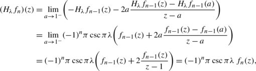
where we have used the fact that n−1+λ<0. Now observe that the functions f n satisfy
$$\int_{C}f_n(t)t^{\lambda-2}=0, \quad0\leq n\leq N.$$This follows, for instance, directly from Theorem 3.1, since f n are eigenfunctions for both H λ and D 1,λ .
- Proof of Step 2.:
-
Let \(\mathcal{M}_{\mu}=\ker(H_{\lambda}-\mu I)\) be a nonzero eigenspace with the additional property that
$$ \int_{C}f(t)t^{\lambda-2}\, \mathrm{d}t=0,\quad f\in\mathcal{M}_{\mu }.$$(4.7)By Theorem 3.1 and Lemma 4.2, we have that \(D_{1,\lambda}\mathcal{M}_{\mu}\subset\mathcal{M}_{\mu}\), and by Lemma 4.5, \(\mathcal{M}_{\mu}\) has finite dimension. The eigenfunctions of \(D_{1,\lambda} \vert \mathcal{M}_{\mu}\) must be the form provided by Proposition 3.2, and as eigenfunctions of H λ they must extend analytically in ℂ∖[1,∞). This implies that the functions in question belong to the set {f n :0≤n≤N}. Now another application of Proposition 3.2 shows that the equation
$$D_{1,\lambda}g-\nu g=f_n$$cannot have solutions analytic near −1. Thus we conclude that \(\mathcal{M}_{\mu}\) is spanned by a subset of {f n :0≤n≤N}, which proves Step 2.
- Proof of Step 3.:
-
We need to show that if μ∈ℂ∖{0} and f∈ker(H λ −μI) with
$$\int_{C}f(t)t^{\lambda-2}\, \mathrm{d}t\neq0 ,$$then
$$\dim\ker(H_{\lambda}-\mu I)=1$$and f is an eigenfunction of D 2,λ . To verify this statement, we use (4.3) again to conclude that
$$\mu(1-z)f(z)=\frac{1}{\kappa}\int_{C}f(t)t^{\lambda-2}\, \mathrm{d}t +\bigl(H_{\lambda-1}(z-1)f\bigr) (z),$$which implies that (H λ−1+μI)X contains the constants.
If dimker(H λ −μI)≥2, then we can find a function g∈ker(H λ −μI) with g≠0 and
$$\int_{C}g(t)t^{\lambda-2}\, \mathrm{d}t= 0.$$Now an application of (4.3) to g shows that
$$\mu(1-z)g(z)=H_{\lambda-1}(z-1)g(z).$$By Lemma 4.5, we obtain that \((1-z)g\in\ker (H_{\lambda-1}+\mu I )\bigcap\mathcal{H}^{\infty}\), which leads to a contradiction by Lemma 4.4. Thus ker(H λ −μI) is spanned by f and by Theorem 3.3, f must be an eigenvalue of D 2,λ and Step 3 is proved. This completes the proof of the theorem. □

References
Andrews, G.E., Askey, R., Roy, R.: Special Functions. Cambridge University Press, Cambridge (1999)
Diamantopoulos, E., Siskakis, A.: Composition operators and the Hilbert matrix. Studia Math. 140, 191–198 (2000)
Duren, P.L.: Theory of H p spaces. Academic Press, New York (1970)
Hill, C.K.: On the singly-infinite Hilbert matrix. J. Lond. Math. Soc. 35, 17–29 (1960)
Lebedev, N.N.: Special Functions and Their Applications. Dover, New York (1972)
Luecking, D.H.: Forward and reverse Carleson inequalities for functions in Bergman spaces and their derivatives. Am. J. Math. 107, 85–111 (1985)
Maier, R.S.: On reducing the Heun equation to the Hypergeometric equation. J. Differ. Equ. 213, 171–203 (2005)
Rainville, E.D.: Special Functions. Chelsea, Bronx (1971). Reprint of the 1960 first edition
Rosenblum, M.: On the Hilbert matrix. I. Proc. Am. Math. Soc. 9, 137–140 (1958)
Acknowledgements
The authors would like to thank B. Shapiro for his helpful comments.
Research partially supported by Plan Nacional I+D+I Grant No. MTM2009-09501 and Junta de Andalucía FQM-260 and P06-FQM-02225.
Author information
Authors and Affiliations
Corresponding author
Additional information
Communicated by Erik Koelink.
Rights and permissions
About this article
Cite this article
Aleman, A., Montes-Rodríguez, A. & Sarafoleanu, A. The Eigenfunctions of the Hilbert Matrix. Constr Approx 36, 353–374 (2012). https://doi.org/10.1007/s00365-012-9157-z
Received:
Revised:
Accepted:
Published:
Issue Date:
DOI: https://doi.org/10.1007/s00365-012-9157-z
Keywords
- Hilbert matrix
- Integral operator
- Eingenvalues
- Eigenfunctions
- Differential operators
- Hypergeometric function
- Associated Legendre functions of the first kind