
Abstract
We implement a semi-analytic scheme for numerically computing high order polynomial approximations of the stable and unstable manifolds associated with the fixed points of the normal form for the family of quadratic volume-preserving diffeomorphisms with quadratic inverse. We use this numerical scheme to study some hyperbolic dynamics associated with an invariant structure called a vortex bubble. The vortex bubble, when present in the system, is the dominant feature in the phase space of the quadratic family, as it encloses all invariant dynamics. Our study focuses on visualizing qualitative features of the vortex bubble such as bifurcations in its geometry, the geometry of some three-dimensional homoclinic tangles associated with the bubble, and the “quasi-capture” of homoclinic orbits by neighboring fixed points. Throughout, we couple our results with previous qualitative numerical studies of the elliptic dynamics within the vortex bubble of the quadratic family.
1 Introduction
When studying the qualitative dynamics of a three-dimensional, volume-preserving discrete-time dynamics system, standard phase space sampling techniques are rarely sufficient. The reason is that such systems do not admit attractors; thus, a typical bounded orbit is an amorphous cloud in phase space, which may cast little light on the geometry of the dynamics. In order to understand the phase space geometry of volume-preserving systems, it is desirable to study the embedding of one- and two-dimensional invariant manifolds. In volume-preserving discrete dynamical systems, two important classes of invariant manifolds are elliptic invariant circles and their associated invariant tori; and hyperbolic invariant manifolds associated with stable and unstable eigenspaces of fixed points. (Other important examples are hyperbolic invariant circles and their associated two-dimensional stable and unstable manifolds, as well as hyperbolic periodic points and their associated stable and unstable manifolds, but these are not treated here.)
In Lomelí and Meiss (1998), a five-parameter family of quadratic volume-preserving maps is given, and it is shown that the family is a normal form for quadratic volume-preserving diffeomorphisms with quadratic inverse. The family is put forward as a natural generalization to three dimensions of the classical area-preserving Hénon family (Hénon 1969). The quadratic family admits at most two fixed points, depending on parameters. Because the map preserves volume, the fixed points are generically hyperbolic, and their two-dimensional stable and unstable manifolds can intersect in such a way as to enclose a region in the phase space.
This region is sometimes referred to as a resonance zone (Lomelí and Meiss 1998, 2000, 2009). At many parameter values there exists an elliptic invariant circle inside the resonance zone which is surrounded by a family of invariant tori (Dullin and Meiss 2009). In this situation the resonance zone is called a vortex bubble. The intersection of the two-dimensional stable and unstable manifolds of the pair of fixed points forms “lobes” whose volume can be quantitatively related to the measure of the set of bounded orbits inside the vortex bubble (Lomelí and Meiss 2009).
The present work addresses two distinct but related issues. Section 2 provides an overview of the computational aspects of the Parameterization Method of Cabré et al. (2003a, 2003b). Section 4 then illustrates the application of these manifold computations to the study of the vortex-bubble geometry in the volume-preserving quadratic family.
In Sect. 2 we begin by discussing in detail the construction of high order polynomial approximations for local stable and unstable manifolds of a fixed point associated with either a single real eigenvalue or a pair of real distinct eigenvalues. In the explicit setting of the volume-preserving quadratic family, we derive “by hand” the equations which implicitly define the polynomial coefficients, and provide numerically verifiable conditions under which the implicit equations are uniquely solvable to all orders. Furthermore, we discuss practical considerations such as deciding the numerical domain of the resulting polynomial approximations. When we supplement the algorithms developed in Sect. 2 with the algorithms for computing two-dimensional stable/unstable manifolds associated with a pair of complex conjugate eigenvalues developed in Mireles James and Lomelí (2010), we are able to accurately compute all the stable/unstable manifolds at a generic hyperbolic fixed point in the quadratic family.
Section 4 functions as a sequel to Dullin and Meiss (2009). That work provides a thorough qualitative study of the regular or “elliptic” dynamics inside the vortex bubble of the volume-preserving quadratic family. The present work provides a parallel study of the irregular, hyperbolic, and chaotic dynamics near the vortex bubble. While Sects. 2 and 4 are written so that they could be read independently, Sect. 2 is essential in order to explain how the results of Sect. 4 are obtained. Similarly, Sect. 4 serves as a case study in the application of the Parameterization Method when studying the phase space geometry of invariant manifolds in a three-dimensional discrete-time dynamical system. Finally, Sect. 3 is a brief description of the algorithms used to compute the homoclinic connecting orbits studied in Sect. 4.
1.1 Context of the Current Work Within the Existing Literature
There is a vast literature on the numerical computation of invariant manifolds in dynamical systems; even an overview of the relevant literature is beyond the scope of this work. We refer to the recent survey article Krauskopf et al. (2005) for an exposition of several numerical methods for computing two-dimensional stable and unstable manifolds associated with hyperbolic equilibria of vector fields, and note that a more complete review of the literature can be found therein.
The Parameterization Method developed in Cabré et al. (2003a, 2003b, 2005), provides a general framework for studying nonresonant stable/unstable manifolds associated with hyperbolic fixed points of diffeomorphisms and equilibria of vector fields. We note that the Parameterization Method is not discussed in Krauskopf et al. (2005); hence we treat the method thoroughly in Sect. 2. In addition to the applications discussed here, we mention that the method has been applied to the computation of hyperbolic invariant tori, their breakdown, and the computation of their stable/unstable manifolds (Haro and de la Llave 2006a, 2006b; Fontich et al. 2009). The Parameterization Method can also be used to prove constructive KAM theorems which avoid the use of action-angle coordinates (de la Llave et al. 2005), and extended to facilitate the computation of center manifolds such as those associated with parabolic fixed points (Baldomá et al. 2007). From a formal point of view, the computational aspects of the Parameterization Method are similar in spirit to the techniques of “automatic differentiation” (see Bücker and Corliss 2006 for a very thorough review of the automatic differentiation literature).
The family of maps studied in this work is called the volume-preserving Hénon family, and it has been studied extensively from a dynamical systems point of view (see, for example, Lomelí and Meiss 1998; Dullin and Meiss 2008, 2009; Gonchenko et al. 2006 and the references in these). It was shown in Lomelí and Meiss (1998) that the quadratic family can be put into normal form by an affine change of variables. Then when studying the dynamics of the quadratic family, it is enough to study the dynamics of the resulting five-parameter normal form. A thorough discussion of the literature surrounding the quadratic family and its normal form can be found in Dullin and Meiss (2009). The reference just mentioned also contains a detailed numerical study of the “elliptic” dynamics of the quadratic family, i.e., the dynamics associated with stable invariant circles and tori. In the sequel we will frequently refer to the numerical results therein.
For a large range of parameters, the quadratic family admits “vortex-bubble” dynamics (Dullin and Meiss 2009). A vortex bubble is characterized by the presence of a toroidal convective roll (family of invariant tori), with “eyes” (fixed points) located on the top and bottom of the hole in the torus, and where the two-dimensional stable and unstable manifolds of the fixed points enclose the tori, forming a “bubble.” The resulting dynamics are qualitatively similar to those of the Hills vortex of fluid dynamics (Sotiropoulos et al. 2001), or the spheromak of plasma physics (MacKay 1994). The phase space dynamics are similar to those of what is sometimes called a “vortex ring” in the plasma literature (Archer et al. 2008).
Vortex dynamics are also discussed widely in the fluid and plasma physics literature (see, for example, Krutzsch 1939; Crow 1970; Archer et al. 2008 for more complete references), and the bubble structure present in the dynamics of the quadratic family is qualitatively similar to much more complicated models of physical phenomena. Examples include tornados (Peikert and Sadlo 2007), turbulence in stirred fluids (Shadden et al. 2007), and tokamak dynamics (Hayashi et al. 2001).
We note that while the references just mentioned actually discuss plasma and fluid models based on differential equations rather than maps, if one were to perturb for example the models of Sotiropoulos et al. (2001) with a τ-periodic forcing function and study the time-τ map, the resulting dynamics would be similar to the Lomelí Family studied here. On the other hand we remark that it is possible to implement a version of the Parameterization Method for differential equations as in van den Berg et al. (2011), Lessard et al. (2013), Johnson and Tucker (2011). Using these techniques one could obtain results similar to ours by working directly with the vector fields of Sotiropoulos et al. (2001), Hayashi et al. (2001), Shadden et al. (2007).
Vortex dynamics are studied in the applied mathematics literature in connection with the phenomenon of “chaotic advection” or “chaotic transport” (Kaper and Wiggins 1991; Raynal and Wiggins 2006; Davies et al. 2008; Neishtadt et al. 1998; Mezić 2001; Mullowney et al. 2005, 2008; Chernikov et al. 1991). The vortex-bubble structure in diffeomorphisms has been studied theoretically from the point of view of stable/unstable manifold theory in Lomelí and Ramírez-Ros (2008), and from the view of Melnikov theory in Lomelí and Meiss (1998). Geometric invariants of the bubble associated with the “lobe-volume” are computed in Lomelí and Meiss (2009). Mireles James and Lomelí (2010) gives a numerical method for computing Taylor expansions of the arcs which form at the intersection of stable and unstable manifolds making up the bubble.
Since (Smale 1965) there has been tremendous interest in homoclinic tangles, which are transverse intersections of the stable and unstable manifolds of a fixed point of a diffeomorphism. It is well known that the presence of a homoclinic tangle implies not only the existence of a homoclinic orbit, but also the existence of chaotic dynamics in a neighborhood of the homoclinic orbit. Efficient numerical methods for computing homoclinic orbits appear as early as Beyn and Kleinkauf (1997a, 1997b). In the sequel we employ a version of the Beyn and Kleinkauf (1997a) algorithm which exploits the high order polynomial approximations of the stable and unstable manifolds derived using the Parameterization Method.
The present work is also closely related to Makino and Berz (2003), Berz and Hoffstätter (1998), and especially to Newhouse et al. (2008). In the last reference, a numerical technique for computing high order Taylor expansions of the stable and unstable manifolds is developed, and applied to the dissipative Hénon mapping of the plane at the classical parameters. Their method is built on the same principles as the Parameterization Method, but they globalize the manifolds by repeatedly composing the polynomial approximations with the Hénon map in order to obtain chart maps of larger and larger segments of the one-dimensional manifolds. These globalized manifolds are used to compute a large number of homoclinic intersections, and by studying these intersections the authors can provide mathematically rigorous bounds on the topological entropy of the Hénon attractor. Their study is implemented using the software package COSY (Berz and Makino 2012).
Finally, a word about mathematical rigor. While the present work focuses on classical floating point computations which are used in order to obtain purely qualitative information about the volume-preserving quadratic family, note that the Parameterization Method is well suited for computer-assisted proofs. For example, it is possible, using a combination of a posteriori functional analytic methods and interval arithmetic, to obtain mathematically rigorous bounds on both the radius of convergence of the formal series and the truncation error introduced by representing the chart map for the stable or unstable manifolds with polynomials (of finite order). The reader interested in the details and implementation of such computer assisted arguments should consult Mireles James and Mischaikow (2013) (for maps) and van den Berg et al. (2011), Johnson and Tucker (2011) (for flows). Of course convergence and regularity of the formal series is treated from a purely theoretical prospective in Cabré et al. (2003a, 2003b, 2005). Other methods for obtaining rigorous containment of invariant manifolds based on topological rather than analytic arguments can be found for example in Neumaier and Rage (1994), Newhouse et al. (2008), Arioli and Zgliczyński (2001), Zbigniew and Zgliczyński (2001).
Remark 1.1
(Comparison with Krauskopf et al. 2005)
It is worth a moments time to consider more closely the relationship between the Parameterization method of Cabré et al. (2003a, 2003b, 2005), van den Berg et al. (2011), Johnson and Tucker (2011), Mireles James and Mischaikow (2013) as used in the present work, and the methods of Krauskopf et al. (2005). Our primary remark is to stress that these should be viewed as complementary rather than competitive methods. The reason for this is that the methods discussed in Krauskopf et al. (2005)—geodesic level sets, BVP continuation of trajectories, computation of fat trajectories, PDE formulation with ordered upwind method, and even the second stage (growth) of the box covering method—are all methods for globalizing a local stable or unstable manifold patch. The authors use the linear approximation of the manifold given by the (un)stable eigenspace as the initial input to their algorithms, but theoretically what is actually required in order to start their methods is any initial approximation of the local manifold.
The Parameterization method on the other hand is a general method for computing high order expansions of the local manifolds without iterating/integrating the dynamical system. One advantage of this approach over the straightforward linear approximation of the manifold is that the stagnant and well understood dynamics close to the fixed point are swallowed up into the polynomial. See for example the upper left hand frame of Fig. 6. The surface and arc in this frame are obtained as the image of the polynomial parameterizations only. No iteration has been performed to obtain this picture. Similarly the top annulus in the upper left and right frames, and the lower left frame of Fig. 10 is the image of a fundamental domain in parameter space under only the polynomial parametrization.
If the methods of Krauskopf et al. (2005) were to be initialized using the high order local manifolds given by the Parameterization Method the results would be better than those obtained initializing with the linear approximation. This is because we can only iterate or integrate the dynamical system accurately for a finite amount of time. Then it is better not to spend these iterates computing the local manifold from the linear approximation, and instead to save our iterates up for computing truly global dynamics. In this sense the Parameterization Method can be seen as a “pre-conditioner” for the globalization methods of Krauskopf et al. (2005) (or for any other globalization scheme based on iteration/integration which one could propose). This kind of preconditioning is especially useful in systems like the Lomelí Family where for the interesting parameter values the linear dynamics at the fixed points are especially slow.
Combining the Parameterization Method with one or more of the industrial strength globalization methods of Krauskopf et al. (2005) would enhance the utility of both works and is an exciting topic for future study. We note for the expert that these remarks are especially enticing in the case of the method of fat trajectories, as the parameterization method can be used to obtain both the tangent space and the curvature at any point on the local patch, even with rigorous error bounds. We also remark for the expert that in the sequel we exploit only naive globalization schemes (straightforward iteration of fundamental domains) which have notorious shortcomings. However the preconditioning provided by the Parameterization Method provides sufficient stabilization that the resulting globalized manifolds meet the needs of the present work.
1.2 Background: Quadratic Volume-Preserving Maps
We are concerned with the five-parameter family of (quadratic) volume-preserving diffeomorphisms f:ℝ3→ℝ3 given by
where Q is the quadratic function
The family was introduced in Lomelí and Meiss (1998) as an analog of the two-dimensional area-preserving Hénon map. We will refer to it as the Lomelí family, or simply the Lomelí map when it is understood that the parameters are fixed.
We note the following useful facts.
-
(a)
When τ 2−4α>0 the map has a pair of (real) distinct fixed points p ±∈ℝ3
$$p_{\pm} = \left ( \begin{array}{c} x_{\pm} \\ x_{\pm} \\ x_{\pm} \\ \end{array} \right ), $$where
$$x_{\pm} = \frac{-\tau \pm \sqrt{\tau^2 - 4 \alpha}}{2}. $$These are the only possible fixed points of the family.
-
(b)
The map is volume preserving, i.e., \(|\operatorname{det}(Df(p))| = 1\), for all p∈ℝ3. Then, for example, at either of the fixed points p ± the generic stability situation will be either two unstable and one stable eigenvalue, or vice versa (as the product of the three eigenvalues is required to be 1). The two eigenvalues with the same stability type (stable or unstable) are generically either real and distinct, or a complex conjugate pair.
-
(c)
The Jacobian differential of the Lomelí family is
$$Df(x,y,z) = \left ( \begin{array}{c@{\quad }c@{\quad }c} 2 a x + by + \tau & 2cy + bx & 1 \\ 1 & 0 & 0 \\ 0 & 1 & 0 \\ \end{array} \right ). $$
In Dullin and Meiss (2009), the authors make an affine change of coordinates to the Lomelí map, putting it in the form
where \(P(x,y) = \bar{a} x^{2} + \bar{b} xy + \bar{c} z^{2}\). We will refer to this as the Dullin–Meiss form of the map. This form has the advantage that the two fixed points are located on the z-axis at \(\pm \sqrt{\epsilon/{\bar{a}}}\). Nevertheless, we focus our studies on the classic Lomelí form of the map, largely so that we can exploit the computational tools developed in Mireles James and Lomelí (2010).
Given a set of parameters in Dullin–Meiss form, it is possible to transform to a Lomelí map with the parameters

These transformations allow us to relate the numerical studies carried out in this work, where we work with the Lomelií form of the map, with the numerical studies in Dullin and Meiss (2009).
2 Parameterization Method for Stable/Unstable Manifolds of Fixed Points
Suppose that f:ℝn→ℝn is a diffeomorphism with a fixed point p∈ℝn, and that the differential Df(p) is conjugate to a linear isomorphism A:ℝn→ℝn with
where \(A_{\mathrm{s}}:\mathbb{R}^{n_{\mathrm{s}}} \rightarrow \mathbb{R}^{n_{\mathrm{s}}}\) and \(A_{\mathrm{u}}:\mathbb{R}^{n_{\mathrm{u}}} \rightarrow \mathbb{R}^{n_{\mathrm{u}}}\) are linear isomorphisms having ∥A s∥<1, ∥A u∥>1, and n s+n u=n. Let \(E_{\mathrm{s}} = \operatorname{range}(A_{\mathrm{s}})\) and \(E_{\mathrm{u}} = \operatorname{range}(A_{\mathrm{u}})\) denote the resulting n s- and n u-dimensional invariant linear subspaces of ℝn.
The stable manifold theorem (see, for example, Palis and de Melo 1982; Robinson 1999; Katok 2012) states that the sets
and
are smooth invariant immersed (but typically not embedded) disks tangent respectively to E s and E u at p. When Df(p) is diagonalizable, the matrices A s and A u can be taken to be the diagonal matrices containing the stable and unstable eigenvalues of Df(p) respectively. The Parameterization Method Cabré et al. (2003a, 2003b, 2005) is a method for computing polynomial expansions for some chart maps of W s,u(p); specifically, chart maps for neighborhoods of p. Such neighborhoods are called local stable/unstable manifolds and are denoted by \(W_{\mathrm{loc}}^{\mathrm{s},\mathrm{u}}(p)\) respectively.
2.1 Parameterization for One-Dimensional Stable and Unstable Manifolds
Let p∈ℝn, and f:ℝn→ℝn be real analytic and invertible on B ρ (p)⊂ℝn, ρ>0. Suppose that f(p)=p, that Df(p) has n−1 eigenvalues \(\{\lambda^{\mathrm{u}}_{1}, \ldots, \lambda^{u}_{n-1} \}\) with |λ i |>1, 1≤i≤n−1, and that Df(p) has a single eigenvalue λ with |λ|<1. Let ξ λ ∈ℝn be an eigenvector of λ. As mentioned above, the stable manifold theorem gives that W s(p) is a one-dimensional smooth (analytic) manifold tangent to ξ λ at p.
The goal of the Parameterization Method in this setting is to compute a smooth injection P:[−τ,τ]⊂ℝ→ℝn having
-
(a)
P(0)=p,
-
(b)
P′(0)=ξ λ ,
-
(c)
and
$$ f \bigl[P(\theta)\bigr] = P(\lambda \theta) $$(2.1)
for all θ∈[−τ,τ]. Note that any P satisfying these conditions, P([−τ,τ]) is an immersed arc through p tangent to ξ λ at p, with f∘P([−τ,τ])⊂P([−τ,τ]). It follows that the ω-limit set of \(\operatorname{image}(P)\) under f is 0, so that the image of P is a local stable manifold about p, or
In general, we will be unable to compute P in closed form. Instead, we note that P satisfies a (functional) initial value problem with analytic data. Then it is natural to assume that P has the power series expansion
with v 0=p and v 1=ξ λ , and we then try to determine the unknown coefficients v n . (Throughout the sequel θ is a real, rather than angular variable.) One way to proceed is to insert Eq. (2.2) into Eq. (2.1), Taylor expand f, and analytically compute recurrence relations for the coefficients of P. This is the approach we pursue below. Another approach, based on Taylor models, is given in Newhouse et al. (2008), while a Newton scheme for computing the coefficients of P is implemented in Mireles James and Lomelí (2010).
2.2 Example: 1D Manifolds for the Lomelí Map
Consider again the Lomelí map
and let
where the fixed points p ± of the Hénon family are known explicitly, and the associated eigenvalue can be computed explicitly either analytically or numerically. Then \((v_{0}^{1}, v_{0}^{2}, v_{0}^{3})^{\mathrm{T}} = p_{\pm}\), and \((v_{1}^{1}, v_{1}^{2}, v_{1}^{3})^{\mathrm{T}} = \xi_{\lambda}\) are the zeroth and first order power series coefficients.
Upon inserting power series into the functional equation
we have that
on the left, and
on the right. Equating the second and third components of the left- and right-hand sides gives
and
Upon matching like powers we obtain
The first component equation is more involved. Expanding the left-hand side of the first component and utilizing the Cauchy product formula gives

Equating like powers gives that

for n≥2. Here we have removed from the sum any terms containing \(v_{n}^{1}\), or \(v_{n}^{2}\). We isolate the n-th coefficients on the left-hand side of the equality in order to obtain

Combining the three component equations in matrix form gives
where
and
Note that if we let y n =(s n ,0,0)T, then the matrix equation has the form
where y n is a known quantity depending recursively on terms of order less than n. This can be seen by recalling the formula for the Jacobian of f from Sect. 1.2, evaluating the Jacobian at p ±, and recalling that \((v_{0}^{1}, v_{0}^{2}, v_{0}^{3}) = p_{\pm}\). Equation (2.5) is called the homological equation for the stable manifold.
The coefficient v n solves the homological equation, and is well defined precisely when A n is invertible. But A n is the characteristic matrix Df(p)−λ n I of Df(p), and this is invertible precisely when λ n is not an eigenvalue of Df(p ±). Since |λ|<1, and the remaining eigenvalues {λ i } are assumed to have norm greater than one, we have that λ n is not an eigenvalue as long as n≥2. But these are exactly the n for which we want to solve the equation, as the constant and first order terms are already constrained. Then the series solution ∑v n θ n=P(θ) is formally well defined to all orders.
Remark 2.1
-
The homological equation for a one-dimensional unstable manifold is exactly the same, except that λ must be the unstable eigenvalue.
-
Since the choice of the length of ξ λ =v 1 is free, the solution P is not unique. However, once the length of the eigenvector is fixed, all remaining terms are determined uniquely by Eq. 2.5), as the matrix is always invertible. Then the formal solution P is unique up to the magnitude of v 1=ξ λ . This can be seen as a rescaling of P.
-
The computation above provides a numerical scheme for computing approximations to the stable manifold. Namely, we can compute a polynomial P N which approximates P to any desired finite order by recursively solving the homological equation (2.5) for 2≤n≤N.
-
In the present work we are not concerned with the convergence of the formal series whose coefficients are defined by the homological equation (2.5). Rather, we are interested in determining when a finite number of terms of P provides a reliable numerical approximation to a local stable/unstable manifold. Nevertheless, the formal series do converge, as shown in Cabré et al. (2005). In that reference, and under the assumptions above, the parameterization power series are shown to converge to entire functions.
2.3 2D Manifolds of the Lomelí Map
In order to parameterize the two-dimensional stable manifold associated with a pair of real, distinct eigenvalues λ 1, λ 2, of Df(p ±), having 0<|λ 1|<|λ 2|<1, we choose eigenvectors ξ 1 and ξ 2 associated with λ 1 and λ 2, and assume that the parameterization P:ℝ2→ℝ3 has the power series expansion
where v mn ∈ℝ3 are coefficients having
and the remaining v mn , m+n≥2, are determined by requiring that P satisfy the functional equation
If we let \(v_{mn} = (v_{mn}^{1}, v_{mn}^{2}, v_{mn}^{3})^{\mathrm{T}}\), then a computation similar to that given in Sect. 2.2 shows that the coefficients for the two-dimensional manifolds in the Lomelí map solve the homological equation
where
and
for s=1,2,3.
Remark 2.2
-
As in the one-dimensional case, this is the correct homological equation for both the stable and unstable parameterizations.
-
If a fixed point of the Lomelí map has a complex conjugate pair of eigenvalues λ and \(\bar{\lambda}\), then we complexify and proceed almost as in the one-dimensional case. More precisely, we take P to have the form
$$P(x,y) = \sum_{n=0}^{\infty} \sum _{m=0}^{\infty} v_{mn} (x+\mathrm{i}y)^m (x - \mathrm{i}y)^n \equiv \bar{P}(z, \bar{z}), $$where z=(x+iy) and v mn ∈ℂ3. Then we impose that P solve the invariance equation
$$f\bigl[\bar{P}(z, \bar{z})\bigr] = \bar{P}(\lambda z, \bar{\lambda} \bar{z}). $$A thorough discussion of the complex conjugate case, along with implementation for the Lomelí map, is found in Mireles James and Lomelí (2010). In particular, ones finds that \(v_{nm} = \overline{v_{mn}}\) so that the image of P(x,y) is real when (x,y)∈ℝ2, and we obtain the real local (un)stable manifold. We employ the numerical methods developed in Mireles James and Lomelí (2010) without further comment whenever needed in the sequel.
-
Note that the homological equation for the two-dimensional stable/unstable parameterization has the form
$$\bigl[Df(p_{\pm}) - \lambda_1^m \lambda_2^n I\bigr] v_{mn} = \left ( \begin{array}{c} -s_{mn} \\ 0 \\ 0 \\ \end{array} \right ), $$which is similar to the one-dimensional situation. Then the coefficients of the formal series exist uniquely for all m,n with m+n≥2, so long as the following nonresonance condition is satisfied:
$$\lambda_1^m \lambda_2^n \neq \lambda_i $$for i=1,2. But since 0<|λ 2|<|λ 2|<1 we have that

It follows that if
$$N > \frac{\ln|\lambda_1|}{\ln|\lambda_2|}, $$and m+n≥N, then there are no resonances. So \(\lambda_{2}^{n} \neq \lambda_{1}\) for 2≤n≤N−1 is enough to guarantee that the parameterization coefficients are formally well defined to all orders. These nonresonance conditions are satisfied for generic parameter sets for the Lomelí family. Similar comments can be made for diffeomorphisms in arbitrary dimensions. See Cabré et al. (2003a, 2005) for details.
In practice, we make sure to numerically compute P N to at least order N>ln|λ 1|/ln|λ 2|. If the system has resonances (or even if the system is roughly machine epsilon close to a resonance), then one of the matrices defining a parameterization coefficient will be noninvertible (or poorly conditioned) and the numerical computation will fail (for example, in MatLab attempting to solve a poorly conditioned linear system leads to a warning). However, if we are able to compute the coefficients numerically to order N (without warning), then we are assured there are no resonances lurking at orders greater than N. If mathematically rigorous enclosures of the polynomial coefficients are required, then the homological equations can be solved using interval methods, as in Mireles James and Mischaikow (2013), van den Berg et al. (2011).

2.4 Numerical Domain for the Polynomial Approximation
Suppose that we have recursively solved Eq. (2.5) up to a fixed finite order N. Then we have a polynomial
which approximates the true parameterization P. While any truncated approximation P N is entire (as P N is a polynomial), we cannot expect P N to approximate P well for all τ∈ℝ. Instead, we will determine a smaller domain on which the approximation is actually “good.” The following definition makes this precise.
Definition 2.1
Let ϵ>0 be a prescribed tolerance. We call the number τ>0 an ϵ-numerical radius of validity for the approximation P N if
Remark 2.3
-
In practice, numerical experimentation is enough to select a good τ.
-
We have the bound
$$ \operatorname{Error}_{\tau}(P_N) \leq \sum _{n=0}^{\infty} |C_n - D_n |^n \tau^n, $$(2.7)where C n , D n are the power series coefficients of f[P N ] and P N (λθ) respectively. When f is a polynomial, all but finitely many of A n , B n are zero, and Eq. (2.4) is easy to compute numerically. If desired, the bound can be made rigorous by employing interval arithmetic.
-
If τ is an ϵ-numerical radius of validity for a polynomial approximation P N of a stable/unstable parameterization and ϵ is small enough, then we can conclude (under certain weak hypotheses which can be rigorously verified using computer-assisted arguments) that the truncation error ∥P N −P∥ τ <Cϵ, where P is the exact solution of the invariance equation (2.1). This kind of mathematically rigorous a posteriori analysis for the Parameterization Method is discussed in detail in Cabré et al. (2003a, 2005), and implemented for flows generated by vector fields in van den Berg et al. (2011) and for maps in Mireles James and Mischaikow (2013). In particular, an explicit expression for C, in terms of f, N, λ, is obtained in the references. Due to the qualitative nature of the present work, we are not concerned with rigorous computations. In the sequel we will, loosely speaking, simply say that the truncation error of P N on the domain [−τ,τ] is on the order of ϵ whenever τ is an ϵ-numerical radius of validity for P N .
-
The definition of ϵ-numerical radii of validity for higher dimensional manifolds is similar, and is given in Mireles James and Lomelí (2010), Mireles James and Mischaikow (2013), van den Berg et al. (2011).
3 Computing Transverse Intersections and Homoclinic Orbits: Method of Projected Boundary Conditions Meets the Parameterization Method
As an elementary application of the Parameterization Method, we give a general scheme for computing connecting orbits associated with homoclinic tangles in ℝ3 (the scheme generalizes for homoclinic tangles in ℝn in an obvious way). We note that a similar technique for computing heteroclinic arcs in ℝ3 is given and implemented in Mireles James and Lomelí (2010). Software for the scheme developed in this section has been implemented in MatLab, and is used in Sect. 4 to study connecting dynamics in the vortex bubble of the Lomelí map.
In short, our method is to use the Method of Projected Boundary Conditions of Beyn and Kleinkauf (1997a, 1997b) in order to formulate the computation of a connecting orbit as the zero of a certain nonlinear map. A standard Newton iteration is used to compute zeros to roughly machine precision. We simply replace the linear approximations of the stable/unstable manifolds used in Beyn and Kleinkauf (1997a) with the high order polynomial expansions obtained above. When computing a homoclinic orbit which spends a large number of iterations outside a fixed neighborhood of the fixed point, our adaptation of the projected boundary method provides added numerical stability. Such orbits are examined in Sect. 4. We describe the modification in full for the sake of completeness.
Consider a hyperbolic fixed point p∈ℝ3 of the diffeomorphism f:ℝ3→ℝ3, and suppose that Df(p) has two unstable eigenvalues λ 1,λ 2 with |λ 1|,|λ 2|>1, and a stable eigenvalue λ with |λ|<1. Let P s:[−τ,τ]⊂ℝ→ℝ3 and P u:B r(0)⊂ℝ2→ℝ3 be parameterizations of the local stable and unstable manifolds.
Now suppose that W s(p) and W u(p) intersect transversally at a point q∈ℝ3. Then there are parameters \(\bar{t} \in [-\tau, \tau]\), \((\bar{\theta}_{1}, \bar{\theta}_{2}) \in B_{\mathrm{r}}\), and integers n s,n u∈ℕ so that
Since the intersection is transverse at q, the vectors
span ℝ3.
Choose n u, n s∈ℕ and define ϕ:ℝ3→ℝ3 by
and note that a nondegenerate zero of ϕ is a parameter set which satisfies Eq. (3.1).
Denote the variable for ϕ by (θ 1,θ 2,t)=w∈ℝ3. Our goal is to numerically compute a \(\bar{w} \in \mathbb{R}^{3}\) solving \(\phi(\bar{w}) = 0\) by iterating the Newton sequence
Note that the differential Dϕ is given by
where | denotes the operation of adjoining of a column vector to a matrix. The differential is then invertible in a neighborhood of \(\bar{w}\) by the transversality assumption (these vectors span ℝ3 near \(\bar{w}\) so that the matrix has nonzero determinant). Then for \(|w_{0} - \bar{w}|\) small enough, the Newton sequence converges to a true solution \(\bar{w}\) by the standard Newton–Kantorovich theorem (see, for example, Cheney 2001).
Remark 3.1
(Locating an Approximate Orbit)
In practice we must determine the numbers n s,n u∈ℕ in order to define the function ϕ. In many cases it is possible to locate the approximate connecting orbits via some numerical continuation procedure. At other times the approximate orbit can be located via some preliminary numerical experimentation. A procedure which formalizes this experimentation proceeds along the following lines.
-
(a)
Choose discretizations of fundamental domains for W s(p) and W u(p) by using the parameter domains [−τ,τ] and B r(0) and the known linear dynamics given by λ, λ 1, and λ 2.
-
(b)
Compute a fixed iterate n u=C of the two-dimensional fundamental domain, and iterate the one-dimensional fundamental domain until the sets intersect. Since we are working in ℝ3, the intersection is perhaps best detected graphically.
-
(c)
Once a valid pair (n s,n u) has been determined so that the iterates of the fundamental domains appear to intersect in phase space, it is easy to search the discretized parameter sets for triples \((\theta_{1}^{0}, \theta_{2}^{0}, t^{0})\) which map under ϕ near the desired intersection. Then we are ready to apply the Newton scheme.
More precisely, this scheme allows us to find parameters \(w_{0} \equiv (\theta_{1}^{0}, \theta_{2}^{0}, t^{0})\), as well as n s and n u so that ∥ϕ(w 0)∥<δ. In applications, δ need only be on the order of say 10−1 or even 100, as w 0 is the input to the Newton scheme.
Remark 3.2
(Computer-Assisted Proof of Homoclinic Chaos)
Since the Newton–Kantorovich theorem provides a posteriori conditions under which one can conclude the existence of a true zero from an approximate zero, the scheme just described above leads quite naturally to elementary computer-assisted proofs of the existence of chaotic motions. The key to such proofs is that the truncations errors associated with the Parameterization Method can be rigorously bounded. These matters are treated in Mireles James and Mischaikow (2013), where the interested reader can find the complete details and example computations.
4 Hyperbolic Dynamics in the Quadratic Volume-Preserving Family
Consider a hyperbolic fixed-point p∈ℝ3 of a diffeomorphism f:ℝ3→ℝ3. We say that p has stability type (2,1) if Df(p) has two unstable eigenvalues, and one stable eigenvalue (hence a two-dimensional unstable and a one-dimensional stable manifold); and say that p has stability type (1,2) if the situation is reversed. When the Dullin–Meiss parameters are fixed with \(\bar{a} = 1.0\), \(\bar{b} = \bar{c} = 1/2\), μ∈[−4,0], then for a large set of ϵ with 0<ϵ<1 the Lomelí map has one fixed point with stability type (2,1) and the second fixed point with stability type (1,2). These are the parameters studied in Dullin and Meiss (2009), and we conform to this convention throughout the sequel.
In the situation just described, we will use p 0 to denote the fixed point with stability type (2,1), and p 1 to denote the fixed point with stability type (1,2). Then W u(p 0) and W s(p 1) are co-dimension one smooth manifolds (immersed disks even) in ℝ3. These surfaces can intersect in such a way as to enclose some bounded volume, creating a structure called a vortex bubble. See Lomelí and Meiss (1998, 2000, 2009), Lomelí and Ramírez-Ros (2008), Dullin and Meiss (2009) and the introduction. In the remainder of this section we apply the techniques discussed in Sect. 2 to make a qualitative study of the vortex-bubble dynamics of the Lomelí map. In particular, we are interested in visualizing the geometry of the stable and unstable manifolds associated with p 0 and p 1.
4.1 ϵ→0+: “Regular” Dynamics
As ϵ→0+ in the Dullin–Meiss parameters, the dynamics of the mapping become increasingly regular. In fact the system approaches “integrable” in a sense made precise in Dullin and Meiss (2009). The integrable behavior of the quadratic family is studied in detail in Dullin and Meiss (2009) (see especially Sect. 5). For completeness we recall some qualitative details.
At ϵ=0 the two distinct fixed points collapse into a single fixed point which disappears for ϵ<0. When 0<ϵ≪1 the behavior of the mapping is qualitatively similar to the behavior of a time τ map of the integrable spheromak flow; i.e., the phase space is foliated by invariant 2-tori, associated with a single elliptic invariant circle. One fixed point has a two-dimensional stable manifold; the other has a two-dimensional unstable manifold. These two-dimensional manifolds coincide, forming a separatrix. The one-dimensional stable and unstable manifolds coincide as well.
The situation is illustrated in Fig. 1. In terms of the present study, the most important observations are the coincidence of the stable and unstable manifolds of the fixed points, that the dynamics of all orbits in the phase space are understood, and in particular that there are no chaotic motions.

Cut-away view of the “integrable” vortex bubble: The outer blue and red surfaces are the unstable and stable manifolds of p 0 and p 1 respectively. The complementary one-dimensional manifolds are shown as well (the one- and two-dimensional manifolds intersect at the fixed points). In this figure the complementary one- and two-dimensional manifolds coincide. The “resonance bubble” or separatrix formed by the two-dimensional manifolds is cut away to show a pair of invariant tori in the bubble. The outer/larger torus is represented as a green point cloud. A smaller solid yellow torus is shown within. The entire inside of the bubble is foliated by such tori which surround an elliptic invariant circle. The dynamics are “integrable” in the sense that every orbit is on a torus, or a separatrix. All orbits on and inside the bubble are bounded. All orbits outside the bubble are unbounded (Color figure online)
We also note that since the Lomelí map can be seen as a small perturbation of an integrable system for 0<ϵ≪1, perturbative methods provide substantial insight into the dynamics of the small ϵ system. For example, we expect exponential splitting of the one- and two-dimensional manifolds, the persistence of a large measure set of invariant tori, the development of hyperbolic and elliptic secondary invariant tori, and the onset of chaos in the “gaps” between the invariant tori. (Also see Fig. 7 in Dullin and Meiss (2009) for a typical cross section of the “near integrable” behavior of the map.)
4.2 ϵ≫0: Far from Integrable Dynamics
In Sect. 4 of Dullin and Meiss (2009), the authors discuss the dependence of the measure of the set of bounded orbits in the Lomelí map on the parameters μ and ϵ. In particular, it is shown numerically that, for ϵ>0.4, the measure of the set of bounded orbits goes to zero, so that classical phase space sampling reveals no recurrent dynamics. Nevertheless, by visualizing the embedding of the global stable and unstable manifolds, we can show that there are nontrivial invariant dynamics in the region of phase space near the two fixed points.
Consider the situation when ϵ=4.0. In this parameter range there are no stable recurrent sets, and a typical orbit diverges rapidly to infinity. Nevertheless, the map still has the fixed points p 0 and p 1 with (2,1) and (1,2) stability respectively. The image in Fig. 2 illustrates the local dynamics near p 0. The image is generated by one iterate of the two-dimensional local unstable manifold and three inverse iterates of the one-dimensional local stable manifold.

Transverse intersection of the stable and unstable manifolds of p 0 when ϵ=4: two transverse intersections of W s(p 0) and W u(p 0) are visible in the top center of the figure
Two transverse intersections of the stable and unstable manifolds are clearly visible. It follows, by the Smale tangle theorem (Smale 1965; Burns and Weiss 1995), that there is a homoclinic orbit through the intersection, and that in some neighborhood of the homoclinic orbit there is a compact invariant set S on which the dynamics are conjugate to the full shift on two symbols. Then we can conclude there are infinitely many distinct bounded periodic orbits in S, an orbit dense in S, sensitive dependence on initial conditions, and chaotic orbits. We are able to arrive at these conclusions in spite of the fact that, at these parameters, the orbit of a randomly selected initial condition will diverge to infinity.
4.3 Vortex-Bubble Bifurcations in μ
In this subsection, and in our discussion of bifurcations throughout the sequel, it is helpful to consider Fig. 3 in Dullin and Meiss (2009). The figure is reproduced (with permission of the authors) as our Fig. 3. The figure illustrates the dependence of the measure of the set of bounded orbits on the parameters ϵ and μ. In Fig. 3, dark blue regions in parameter space represent Lomelí maps where less than one percent of the orbits sampled remain bounded and dark red regions represent Lomelí maps where the percentage of bounded orbits is larger. Since a set of bounded orbits of positive measure is often indicative of the existence of invariant tori, Fig. 3 also suggests parameters which are most likely to exhibit invariant tori. The approximate bimodality of Fig. 3, for fixed ϵ and varying μ, is the dominant qualitative feature. In this subsection we consider bifurcations of the vortex bubble which occur when the parameter μ is varied for fixed ϵ. The results are given in Fig. 4.

Figure 3 in Dullin and Meiss (2009) (reproduced with permission of the authors). The figure illustrates the density of bounded orbits as a function of the parameters ϵ and μ. A point in parameter space is colored blue if no bounded orbits are observed, and colored increasingly red as the density of bounded orbits increases (Color figure online)

Vortex-bubble bifurcations in μ: μ=−1.383, ϵ=0.11 (top left); μ=−1.75, ϵ=0.1 (top right); μ=−1.8, ϵ=0.1 (center left); μ=−2.0, ϵ=0.8 (center right); μ=−3.0, ϵ=0.1 (bottom left); μ=−3.5 ϵ=0.1 (bottom right)
The six frames of Fig. 4 illustrate six vortex bubbles, corresponding to Dullin–Meiss parameters near the ϵ=0.1 line, with μ equal to −1.383, −1.75, −1.8, −2.0, −3.0, and −3.5 (the corresponding frames read from left to right, top to bottom). Each frame of Fig. 4 shows the globalized unstable manifold of p 0 (blue) and the globalized stable manifold of p 1 (red). In each frame p 0 is in the center left of the frame and p 1 is in the center right (for example, in the bottom left frame, the fixed points are located at the extreme left and right of the surfaces).
The vortex bubbles exhibit rich geometric structure, which can be described qualitatively using the notion of intersection homology. This idea is developed formally in Lomelí and Meiss (2000), but heuristically the idea is that the intersection of the two-dimensional manifolds along the outer boundary of the vortex bubble forms curves which are called the primary intersection of the manifolds. If we choose a fundamental domain for, say the stable manifold, then we have an annulus in parameter space whose boundary circles map from one to the other. The primary intersection curves are pulled back to parameter space and intersected with the annulus. Identifying the boundary circles of the fundamental domain (annulus) yields a torus, and the homotopy class of the intersection curve (now a one-dimensional submanifold of the torus) describes the geometry of the intersection of the stable and unstable manifolds. (This notion generalizes the concept of Melnikov level sets to nonperturbative situations.)
The homotopy class of the primary intersection curve in the torus is a pair of integers (k 1,k 2), where k 1 is the number of times the intersection curve winds around the homology generator of the annulus, and k 2 describes how many times the curve winds around the homology generator created by identifying the boundary curves of the annulus. In terms of phase space dynamics, k 1 describes how many times the intersection winds around the outside of the vortex bubble, measured over a fundamental domain; while k 2 measures the number of distinct “branches” of the fundamental intersection. (The interested reader unfamiliar with these notions can consult (Lomelí and Meiss 2000).)
Figure 4 illustrates the bifurcation of the bubble geometry, and hence the primary intersection, as the parameter μ is decreased from μ=−1.383 in the top left frame, to μ=−3.5 in the bottom figure. Varying μ clearly causes bifurcations in the homotopy type of the primary intersection, as well as in the regularity of the intersection curves themselves (note that in the top left and middle right frames the intersection curves are much smoother or “straighter” than in the top right, middle left, and bottom right frames). The most dramatic bifurcation occurs as μ passes through the blue parameters around μ=−3.0, when it is not clear that the manifolds intersect at all. When we compare with Fig. 3 we see that there are no bounded orbits near these parameters. It is possible that the failure of the manifolds to enclose a region corresponds to the failure of the system to exhibit bounded orbits. However, we note that since the pictures do not represent mathematically rigorous computations and since some regions of the manifolds globalize very slowly while some globalize very rapidly, a more deliberate study is needed to understand completely what is happening near μ=−3.0.
Remark 4.1
(Dynamics inside the Vortex Bubble)
Several of the frames in Fig. 4 illustrate vortex bubbles at parameter sets already studied in Dullin and Meiss (2009). This repetition is deliberate, as combining the results of Dullin and Meiss (2009) with our results increases our understanding of the qualitative dynamics in the bubble. Compare, for example, the first frame of Fig. 4 with the topmost image in Fig. 25 in Dullin and Meiss (2009). The images correspond to the same Dullin–Meiss parameters of the mapping (μ=−1.383, ϵ=0.11), so we know that inside the vortex bubble in the first frame of Fig. 4 there is an invariant period 5 torus (5 distinct tori which map one to another), and that these tori are surrounded by a single primary torus.
Similarly, the fourth frame of Fig. 4 corresponds to (μ=2.0, ϵ=0.08). The dynamics interior to the vortex bubble are illustrated in the right-hand square of Fig. 24 of Dullin and Meiss (2009), and we know that the system has undergone the “string of pearls” bifurcation. The dynamics interior to the bubble are dominated by four copies of the original vortex bubble, strung together in a periodic structure. Also compare Figs. 4 and especially 5 with Fig. 8 of Lomelí and Meiss (1998). The latter figure illustrates the geometry of vortex-bubble bifurcations for a different two-parameter family of volume-preserving maps.

Vortex-bubble bifurcations in ϵ: ϵ=0.1 (top left), ϵ=0.15 (top right), ϵ=0.23 (bottom left), and ϵ=0.75 (bottom right). μ=−2.4 throughout
4.4 Vortex-Bubble Bifurcations in ϵ
Now we fix μ=−2.4 and examine the geometry of the bubble as ϵ varies. Our results are summarized in Fig. 5. What is clear from comparing Fig. 5 with Fig. 3 is that, as ϵ increases, the decrease in the measure in the set of bounded orbits (i.e., the breakdown in the regularity of the dynamics in the bubble) is correlated with an increased irregularity in the geometry of the vortex bubble. The irregularity can be measured quantitatively by studying the homotopy type of the primary intersection. Note also that the disappearance of bounded orbits associated with large ϵ again seems to correspond to the breakdown of the vortex-bubble structure. This is illustrated in the bottom right frame of Fig. 5, where it seems that the manifolds may not enclose a region at all.
Remark 4.2
(Dynamics inside the Vortex Bubble)
The first and third frames of Fig. 5 correspond to values of ϵ=0.1 and ϵ=0.32 respectively. The dynamics inside the vortex bubbles at these parameter values are illustrated in the first and third boxes in Fig. 8 of Dullin and Meiss (2009). Then inside the bubble shown in the first frame of Fig. 5, the dynamics are dominated by a family of primary invariant tori, around which a family of secondary invariant tori are “braided.”
However, inside the vortex bubble of the third frame of Fig. 5, the primary family of tori have disappeared, and Fig. 8 of Dullin and Meiss (2009) suggests that the tori have been replaced by a hyperbolic period 7 saddle point (see caption of Fig. 8 in Dullin and Meiss 2009).
4.5 Geometry of the 1D Stable and Unstable Manifolds, Capture Dynamics, and Three-Dimensional Homoclinic Tangles
In this section we examine the geometry of the one-dimensional stable and unstable manifolds in the Lomelí family, and discuss some qualitative dynamics associated with these manifolds. To begin, we fix the Dullin–Meiss parameters at ϵ=0.08 and μ=−2.0. In Fig. 6 we show the local unstable manifold \(W_{\mathrm{loc}}^{u}(p_{0})\) and four different globalizations of the stable manifold W s(p 0). The one-dimensional unstable manifold of p 1 is similar.

Geometry of one-dimensional manifold (μ=−2.0, ϵ=0.08): Local stable and unstable manifolds of p 0 (top left; red and blue respectively). 95 inverse iterates of the local stable manifold, illustrate the “capture” effect of p 1 (top right). 115 inverse iterates of the local stable manifold show numerous transverse intersections with the local unstable manifold, and imply the existence of a topological horseshoe (bottom left). 135 inverse iterates of the local stable manifold show accumulation of W s(p 0) in itself, as required by the λ-Lemma (Color figure online)
Remark 4.3
(Quasi-Capture Dynamics)
-
(a)
One of the dominant features of the embedding of the one-dimensional manifold is a kind of “quasi-capture” dynamics, which we describe now. By “capture” we mean that an entire fundamental domain of the one-dimensional stable manifold of p 0 passes close to the companion fixed point p 1. When this happens, we say that the one-dimensional manifold W s(p 0) is “captured” by p 1. The term capture is appropriate, as when a segment of W s(p 0) comes close enough to p 1 the dynamics of all the orbits on the segment are dominated by the linear dynamics induced by Df(p 1). Since Df(p 1) has a two-dimensional stable eigenspace and a one-dimensional unstable eigenspace, any orbit which passes close enough to p 1 must leave the neighborhood of p 1 along the two-dimensional stable manifold in backward time.
This is exactly the behavior we see in the second frame of Fig. 6, and in Fig. 7. The latter figure illustrates the smoothness of this transition, as well as the splitting of the one-dimensional manifolds. Note that the closer the segment of stable manifold comes to p 1, the longer the embedding of the manifold is dominated by the linear stable dynamics of Df(p 1). We add the descriptor “quasi” as the capture is only temporary.
Fig. 7 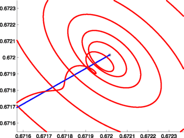
“Quasi-capture” of W s(p 0) by p 1 (red curve and black star respectively). The unstable manifold of p 1 is shown as well (blue curve) (Color figure online)
-
(b)
Recall that the dynamics inside the vortex bubble are illustrated in Fig. 24 of Dullin and Meiss (2009) (the bubble itself is shown in the fourth frame of our Fig. 4). Then the dynamics inside the bubble consist largely of rotational/toroidal dynamics about the x=y=z-line. When ϵ is not too large, this has the effect of forcing the one-dimensional manifolds through the hole of the torus. This forces the close pass between W s(p 0) and the fixed point p 1.
-
(c)
The phenomena just described might be considered a toy model for the “ballistic capture” phenomena which have received much attention in celestial mechanics. See, for example, Belbruno (1993, 1994), Bollt and Meiss (1995), Gomez et al. (2004), Gidea and Masdemont (2007), Senet and Ocampo (2005), Circi and Teofilatto (2001), and the references therein. Ballistic capture occurs, for example, when a projectile launched from the earth enters into a temporary orbit about the moon.
-
(d)
Since an entire fundamental domain of W s(p 0) is quasi-captured by p 1, the amount of time (number of iterates) that the fundamental domain stays in the neighborhood gives a lower bound on the amount of time that any homoclinic orbit spends near p 1 (see also Fig. 8).
Fig. 8 
Homoclinic capture: The image shows the time series for four homoclinic orbits. The parameter values are ϵ=0.2, ϵ=0.32, ϵ=0.75, ϵ=2.0 (from top to bottom) and μ=−2.4 throughout. The orbits illustrate the dependence of the capture time on ϵ. Note that the time scales for the figures are different. Also, looking at the time-series data reminds us that the system can be thought of as a system of three coupled, nonlinear difference equations; thus our methods can also be thought of as a way to compute homoclinic orbits in difference equations


Remark 4.4
(One-Dimensional Tangle Dynamics)
If we continue to inverse-iterate the one-dimensional local stable manifold, then the resulting global manifold W s(p 0) eventually intersects the two-dimensional local unstable manifold of p 1. This is illustrated in the third frame of Fig. 6. The frame clearly illustrates numerous transverse intersections of the stable and unstable manifolds. The existence of such intersections implies, by the Smale tangle theorem (Smale 1965; Burns and Weiss 1995), the existence of a topological horseshoe and in particular bounded chaotic orbits.
The λ-Lemma (Palis and de Melo 1982) further implies that the one-dimensional manifold eventually accumulates on itself. This is illustrated in the final frame of Fig. 6. Moreover, results in topological dynamics show that the closure of W s(p 0) (approximated by the image in the final frame) is a bizarre topological space known as an indecomposable set (see Barge 1987; Kennedy and Yorke 1997).
Remark 4.5
(Homoclinic Orbits)
The existence of a nonempty intersection of the stable and unstable manifolds implies the existence of a homoclinic orbit. We can use the Newton scheme discussed in Sect. 3 to actually compute these homoclinic orbits. The results of such computations are illustrated in Fig. 8. This figure shows time series (x-coordinate versus time), for orbits homoclinic to p 0, computed at ϵ=0.2, ϵ=0.32, ϵ=0.75, and ϵ=2, all with μ=−2.4. (Recall that the vortex bubbles for the second and third of these parameter sets are shown in Fig. 5.)
The frames in Fig. 8 illustrate the minimal duration of the capture dynamics as a function of ϵ. Then we see, for example, that when ϵ=0.2 the homoclinic orbit spends almost 40 iterates in a small neighborhood of p 1 (this appears as the long plateau in the middle of the top frame). However, when ϵ=0.75 (third frame), the orbit only spends three iterates in a small neighborhood of p 1, and when ϵ=2.0 (last frame) the influence of p 1 has almost vanished. Compare this also with Fig. 2, which shows a tangle for ϵ=4.0, and where the stable manifold intersects the local unstable manifold without passing near p 1.
We note that these transverse homoclinic orbits can be computed rigorously using the methods of Mireles James and Mischaikow (2013) and that this leads to a mathematically rigorous proof of the existence of chaotic motions in the Lomelí family.
Remark 4.6
(Two-Dimensional Tangle Dynamics)
Figure 9 illustrates one possible geometry for a homoclinic tangle in three dimensions. The parameter values in this figure are the same as in Mireles James and Lomelí (2010), namely a=0.44, b=0.21, c=0.35, α=−0.25, and τ=−0.3 (here we are using the Lomelí form of the parameters).

The figure illustrates a homoclinic tangle associated with p 0 in the volume-preserving Henon map. This is a three-dimensional analog of the usual planar rendering of tangle dynamics. Note that many transverse intersections of the one- and two- dimensional manifolds are visible, indicating the existence of a three-dimensional version of a Smale horseshoe
In Figs. 10 and 11 we illustrate the embedding of the two-dimensional stable/unstable manifolds in the presence of tangle dynamics. In the first frame of Fig. 10 (top left) we have plotted a fundamental domain for W s(p 1), along with its fifth inverse-iterate (the fundamental domain is the annulus in the top of the frame, and its image is the bent annulus below it). The second frame shows the same fundamental domain, with its tenth inverse-iterate. The effect of the application of ten (inverse) iterates of the map on the fundamental domain is largely one of nonlinear stretching (some parts of the fundamental domain are stretched more than others).

Stretching and folding dynamics: The series of frames show a fundamental domain for the stable manifold of p 1, along with 5 (top left), 10 (top right), and 35 of its iterates. The last frame (bottom right) shows the stable manifold itself. The frames are meant to illustrate the geometry of the two-dimensional stable manifold when a homoclinic tangle is present. The third frame especially illustrates the accumulation of the manifold on itself, due to λ-Lemma effects

Two-dimensional homoclinic tangle: This figure illustrates the immersion of the two-dimensional stable manifold of p 1 at a homoclinic tangle. Note that the image is that of an immersed disk, and suggests the manner in which the manifold is stretched and folded back onto itself by the dynamics. This image can also be seen as a two-dimensional version of the homoclinic tangle which Poincare considered “hard to draw” in the planar case
When we look at the thirtieth (inverse) iterate in the third frame (bottom left) we see a new effect. Here the image of the fundamental domain has been stretched and then folded in on itself. It is essential to note that the third frame illustrates the image of an annulus. The third frame indicates the manner in which the manifold accumulates on itself, as required by the λ-Lemma.
The final frame in the sequence illustrates the global geometry of the stable manifold at this parameter value. The global manifold is, of course, the forward and backward orbit closure of the fundamental domain. An enlarged version of the fourth frame is shown in Fig. 11. The enlarged image is also given some transparency, so that the accumulation of the stable manifold on itself can be clearly seen. The fact that the image in Fig. 11 is the smooth image of a disk highlights the complexity of the dynamics near a three-dimensional homoclinic tangle.
5 Conclusions
We have demonstrated the use of the Parameterization Method as a tool for visualizing unstable/chaotic dynamics in volume-preserving maps. The Parameterization Method is well suited for such studies, as it facilitates computation of local stable and unstable manifolds which are accurate to machine precision. Since the resulting local approximations occupy large regions of phase space bounded away from the fixed point, they minimize the number of iterates needed to globalize the manifolds.
These tools are applied to the study of vortex dynamics arising in the family of quadratic, volume-preserving diffeomorphisms with quadratic inverse. Here our results highlight connection between the measure of the set of bounded orbits observed in Dullin and Meiss (2009) and the qualitative features of the vortex-bubble structure. We further provide geometric evidence for the existence of chaotic motions in the bubble, by exhibiting transverse intersections between the stable and unstable manifolds of fixed points. We also examine the qualitative features of homoclinic orbits, and the accumulation of the one- and two-dimensional manifolds on themselves resulting from a homoclinic tangle in three dimensions.
References
Archer, P.J., Thomas, T.G., Coleman, G.N.: Direct numerical simulation of vortex ring evolution from the laminar to the early turbulent regime. Ann. Phys. 598, 201–226 (2008)
Arioli, G., Zgliczyński, P.: Symbolic dynamics for the Hénon-Heiles Hamiltonian on the critical level. J. Differ. Equ. 171(1), 173–202 (2001)
Baldomá, I., Fontich, E., de la Llave, R., Martín, P.: The parameterization method for one-dimensional invariant manifolds of higher dimensional parabolic fixed points. Discrete Contin. Dyn. Syst. 17(4), 835–865 (2007)
Barge, M.: Homoclinic intersections and indecomposability. Proc. Am. Math. Soc. 101 (1987)
Belbruno, E.: Sun-perturbed earth-to-moon transfers with ballistic capture. J. Guid. Control Dyn. 16, 770–775 (1993)
Belbruno, E.: Ballistic lunar capture transfers using the fuzzy boundary and solar perturbations: a survey. J. Br. Interplanet. Soc. 47, 73–80 (1994)
Berz, M., Hoffstätter, G.: Computation and application of Taylor polynomials with interval remainder bounds. Reliab. Comput. 4(1), 83–97 (1998)
Berz, M., Makino, K.: Cosy infinity (2012). http://www.cosyinfinity.org
Beyn, W., Kleinkauf, J.: The numerical computation of homoclinic orbits for maps. SIAM J. Numer. Anal 34(3), 1207–1236 (1997a)
Beyn, W., Kleinkauf, J.: Numerical approximation of homoclinic chaos. In: Dynamical Numerical Analysis (Atlanta, GA, 1995). Numer. Algorithms 14(1–3), 25–53 (1997b)
Bollt, E., Meiss, J.D.: Targeting chaotic orbits to the moon. Phys. Lett. A 204, 373–378 (1995)
Bücker, H.M., Corliss, G.F.: A bibliography of automatic differentiation. In: Automatic Differentiation: Applications, Theory, and Implementations. Lect. Notes Comput. Sci. Eng., vol. 50, pp. 321–322. Springer, Berlin (2006)
Burns, K., Weiss, H.: A geometric criterion for positive topological entropy. Commun. Math. Phys. 172(1), 95–118 (1995)
Cabré, X., Fontich, E., de la Llave, R.: The parameterization method for invariant manifolds. I. Manifolds associated to non-resonant subspaces. Indiana Univ. Math. J. 52(2), 283–328 (2003a)
Cabré, X., Fontich, E., de la Llave, R.: The parameterization method for invariant manifolds. II. Regularity with respect to parameters. Indiana Univ. Math. J. 52(2), 329–360 (2003b)
Cabré, X., Fontich, E., de la Llave, R.: The parameterization method for invariant manifolds. III. Overview and applications. J. Differ. Equ. 218(2), 444–515 (2005)
Cheney, W.: Analysis for Applied Mathematics. Graduate Texts in Mathematics, vol. 208. Springer, Berlin (2001)
Chernikov, A.A., Neĭshtadt, A.I., Rogal’sky, A.V., Yakhnin, V.Z.: Adiabatic chaotic advection in nonstationary 2D flows. In: Maiakovskiĭ, V. (ed.) Nonlinear Dynamics of Structures, 1990, pp. 337–345. World Sci. Publ., River Edge (1991)
Circi, C., Teofilatto, P.: On the dynamics of weak stability boundary lunar transfers. Celest. Mech. Dyn. Astron. 79, 41–72 (2001)
Crow, S.: Stability theory for a pair of trailing vortices. AAIA J. 8, 2172–2179 (1970)
Davies, P.A., Koshel, K.V., Sokolovskiy, M.A.: Chaotic advection and nonlinear resonances in a periodic flow above submerged obstacle. In: IUTAM Symposium on Hamiltonian Dynamics, Vortex Structures, Turbulence. IUTAM Bookser., vol. 6, pp. 415–423. Springer, Dordrecht (2008)
de la Llave, R., González, A., Jorba, À., Villanueva, J.: KAM theory without action-angle variables. Nonlinearity 18(2), 855–895 (2005)
Dullin, H.R., Meiss, J.D.: Nilpotent normal form for divergence-free vector fields and volume-preserving maps. Physica D 237(2), 156–166 (2008)
Dullin, H.R., Meiss, J.D.: Quadratic volume-preserving maps: invariant circles and bifurcations. SIAM J. Appl. Dyn. Syst. 8(1), 76–128 (2009)
Fontich, E., de la Llave, R., Sire, Y.: Construction of invariant whiskered tori by a parameterization method. I. Maps and flows in finite dimensions. J. Differ. Equ. 246(8), 3136–3213 (2009)
Gidea, M., Masdemont, J.: Geometry of homoclinic connections in a planar circular restricted three-body problem. Int. J. Bifurc. Chaos 17 (2007)
Gomez, G., Koon, W.S., Lo, M.W., Marsden, J.E., Masdemont, J., Ross, S.D.: Connecting orbits and invariant manifolds in the spatial restricted three-body problem. Nonlinearity 17, 1571–1606 (2004)
Gonchenko, S.V., Meiss, J.D., Ovsyannikov, I.I.: Chaotic dynamics of three-dimensional Hénon maps that originate from a homoclinic bifurcation. Regul. Chaotic Dyn. 11(2), 191–212 (2006)
Haro, À., de la Llave, R.: A parameterization method for the computation of invariant tori and their whiskers in quasi-periodic maps: numerical algorithms. Discrete Contin. Dyn. Syst., Ser. B 6(6), 1261–1300 (2006a)
Haro, A., de la Llave, R.: A parameterization method for the computation of invariant tori and their whiskers in quasi-periodic maps: rigorous results. J. Differ. Equ. 228(2), 530–579 (2006b)
Hayashi, T., Mizuguchi, N., Sato, T.: Magnetic reconnection and relaxation phenomena in a spherical tokamak. Earth Planets Space 53, 561–564 (2001)
Hénon, M.: Numerical study of quadratic area-preserving mappings. Q. Appl. Math. 27, 291–312 (1969)
Johnson, T., Tucker, W.: A note on the convergence of parametrised non-resonant invariant manifolds. Qual. Theory Dyn. Syst. 10, 107–121 (2011)
Kaper, T.J., Wiggins, S.: Lobe area in adiabatic Hamiltonian systems. Physica D 51(1–3), 205–212 (1991). Nonlinear science: the next decade (Los Alamos, NM, 1990)
Katok, A.: Introduction to the Modern Theory of Dynamical Systems. Encyclopedia of Mathematics and Its Applications, vol. 54. Cambridge University Press (2012). With a supplementary chapter by Katok and Leonardo Mendoza
Kennedy, J.A., Yorke, J.A.: The topology of stirred fluids. Topol. Appl. 80 (1997)
Krauskopf, B., Osinga, H.M., Doedel, E.J., Henderson, M.E., Guckenheimer, J., Vladimirsky, A., Dellnitz, M., Junge, O.: A survey of methods for computing (un)stable manifolds of vector fields. Int. J. Bifurc. Chaos Appl. Sci. Eng. 15(3), 763–791 (2005)
Krutzsch, C.: Uber eine experimentell beobachtete Erscheinung an Wirbelringen bei ihrer translatorischen Bewegung in wirklichen Flussigkeiten. Ann. Phys. 5, 497–523 (1939)
Lessard, J.P., Mireles James, J.D., Reinhardt, Ch.: Computer assisted proof of transverse saddle-to-saddle connecting orbits for first order vector fields (2013, submitted)
Lomelí, H.E., Meiss, J.D.: Quadratic volume-preserving maps. Nonlinearity 11(3), 557–574 (1998)
Lomelí, H.E., Meiss, J.D.: Heteroclinic primary intersections and codimension one Melnikov method for volume-preserving maps. Chaos 10(1), 109–121 (2000). Chaotic kinetics and transport (New York, 1998)
Lomelí, H.E., Meiss, J.D.: Resonance zones and lobe volumes for exact volume-preserving maps. Nonlinearity 22(8), 1761–1789 (2009)
Lomelí, H.E., Ramírez-Ros, R.: Separatrix splitting in 3D volume-preserving maps. SIAM J. Appl. Dyn. Syst. 7, 1527–1557 (2008)
MacKay, R.S.: Transport in 3D volume-preserving flows. J. Nonlinear Sci. 4, 329–354 (1994)
Makino, K., Berz, M.: Taylor models and other validated functional inclusion methods. Int. J. Pure Appl. Math. 6(3), 239–316 (2003)
Mezić, I.: Chaotic advection in bounded Navier–Stokes flows. J. Fluid Mech. 431, 347–370 (2001)
Mireles James, J.D., Lomelí, H.: Computation of heteroclinic arcs for the volume preserving Hénon map. SIAM J. Appl. Dyn. Syst. 9(3), 919–953 (2010)
Mireles James, J.D., Mischaikow, K.: Rigorous a posteriori computation of (un)stable manifolds and connecting orbits for analytic maps. In: SIADS (2013, to appear)
Mullowney, P., Julien, K., Meiss, J.D.: Blinking rolls: chaotic advection in a three-dimensional flow with an invariant. SIAM J. Appl. Dyn. Syst. 4(1), 159–186 (2005) (electronic)
Mullowney, P., Julien, K., Meiss, J.D.: Chaotic advection and the emergence of tori in the Küppers–Lortz state. Chaos 18(3), 033104 (2008)
Neishtadt, A.I., Vainshtein, D.L., Vasiliev, A.A.: Chaotic advection in a cubic Stokes flow. Physica D 111(1–4), 227–242 (1998)
Neumaier, A., Rage, T.: Rigorous chaos verification in discrete dynamical systems. Physica D 67(4), 327–346 (1994)
Newhouse, S., Berz, M., Grote, J., Makino, K.: On the estimation of topological entropy on surfaces. In: Geometric and Probabilistic Structures in Dynamics. Contemp. Math., vol. 469, pp. 243–270. Amer. Math. Soc., Providence (2008)
Palis, J. Jr., de Melo, W.: Geometric Theory of Dynamical Systems. Springer, New York (1982). An introduction, Translated from the Portuguese by A.K. Manning
Peikert, Sadlo: Topology-Guided Visualization of Constrained Vector Fields. Springer, Berlin (2007)
Raynal, F., Wiggins, S.: Lobe dynamics in a kinematic model of a meandering jet. I. Geometry and statistics of transport and lobe dynamics with accelerated convergence. Physica D 223(1), 7–25 (2006)
Robinson, C.: Dynamical Systems, 2nd edn. Studies in Advanced Mathematics. CRC Press, Boca Raton (1999). Stability, symbolic dynamics, and chaos
Senet, J., Ocampo, C.: Low-thrust variable specific impulse transfers and guidance to unstable periodic orbits. J. Guid. Control Dyn. 28, 280–290 (2005)
Shadden, S.C., Katija, D., Rosenfeld, M., Marsden, J.E., Dabiri, J.O.: Transport and stirring induced by vortex formation. Ann. Phys. 5, 497–523 (2007)
Smale, S.: Diffeomorphisms with many periodic points. In: Differential and Combinatorial Topology (A Symposium in Honor of Marston Morse), pp. 63–80. Princeton Univ. Press, Princeton (1965)
Sotiropoulos, F., Ventikos, Y., Lackey, T.C.: Chaotic advection in three-dimensional stationary vortex-breakdown bubbles: Sil’nikov’s chaos and the devil’s staircase. J. Fluid Mech. 444, 257–297 (2001)
van den Berg, J.B., Mireles James, J.D., Lessard, J.P., Mischaikow, K.: Rigorous numerics for symmetric connecting orbits: even homoclinics for the Gray-Scott equation. SIAM J. Math. Anal. 43, 1557–1594 (2011)
Zbigniew, G., Zgliczyński, P.: Abundance of homoclinic and heteroclinic orbits and rigorous bounds for the topological entropy for the Hénon map. Nonlinearity 14(5), 909–932 (2001)
Acknowledgements
The author was supported by NSF grant DMS 0354567, by a DARPA FunBio grant, and also by the University of Texas Department of Mathematics Program in Applied and Computational Analysis RTG Fellowship, during the preparation of this work. The author would like to thank Professor Rafael de la Llave for his continued encouragement and support as this manuscript evolved. The images in the manuscript are generated using the PovRay ray-tracing software. Thanks go to Dr. Jason Chambless for many helpful suggestions and insights on the use of the PovRay package. The author spent a week in February 2010 visiting the University of Colorado at Boulder Department of Applied Mathematics, and conversations with Professor James Meiss greatly improved and influenced the content of this work. Thanks again to Professors Meiss and Dullin for granting their permission to reproduce Fig. 3 in the present manuscript. Thanks go to Professors Meiss and Curry and also to Mr. Brock Alan Mosovsky and Ms. Kristine Snyder for their hospitality during that visit. Finally, the author thanks Professors de la Llave and Meiss for carefully reading the manuscript and for their many helpful comments and suggestions.
Author information
Authors and Affiliations
Corresponding author
Additional information
Communicated by G. Haller.
Rights and permissions
About this article
Cite this article
Mireles James, J.D. Quadratic Volume-Preserving Maps: (Un)stable Manifolds, Hyperbolic Dynamics, and Vortex-Bubble Bifurcations. J Nonlinear Sci 23, 585–615 (2013). https://doi.org/10.1007/s00332-012-9162-1
Received:
Accepted:
Published:
Issue Date:
DOI: https://doi.org/10.1007/s00332-012-9162-1