
Abstract
We study boundary value problems posed in a semistrip for the elliptic sine-Gordon equation, which is the paradigm of an elliptic integrable PDE in two variables. We use the method introduced by one of the authors, which provides a substantial generalization of the inverse scattering transform and can be used for the analysis of boundary as opposed to initial-value problems. We first express the solution in terms of a 2×2 matrix Riemann–Hilbert problem whose “jump matrix” depends on both the Dirichlet and the Neumann boundary values. For a well posed problem one of these boundary values is an unknown function. This unknown function is characterised in terms of the so-called global relation, but in general this characterisation is nonlinear. We then concentrate on the case that the prescribed boundary conditions are zero along the unbounded sides of a semistrip and constant along the bounded side. This corresponds to a case of the so-called linearisable boundary conditions, however, a major difficulty for this problem is the existence of non-integrable singularities of the function q y at the two corners of the semistrip; these singularities are generated by the discontinuities of the boundary condition at these corners. Motivated by the recent solution of the analogous problem for the modified Helmholtz equation, we introduce an appropriate regularisation which overcomes this difficulty. Furthermore, by mapping the basic Riemann–Hilbert problem to an equivalent modified Riemann–Hilbert problem, we show that the solution can be expressed in terms of a 2×2 matrix Riemann–Hilbert problem whose “jump matrix” depends explicitly on the width of the semistrip L, on the constant value d of the solution along the bounded side, and on the residues at the given poles of a certain spectral function denoted by h(λ). The determination of the function h remains open.
1 Introduction
A method for solving initial-boundary value problems for linear and integrable nonlinear PDEs was introduced in Fokas (1997, 2000) and developed by several authors, see the survey Fokas (2008) and the references therein. This method has already been used for:
-
(a)
linear and integrable nonlinear evolution PDEs formulated on the half line and on a finite interval (Bona and Fokas 2008; Boutet de Monvel et al. 2004; Dujardin 2009; Flyer and Fokas 2008; Fokas 2002a, 2002b; Fokas and Its 1996, 2004; Fokas et al. 2005; Fokas and Lenells 2010; Fokas and Pelloni 2005; Pelloni 2005a, 2004; Treharne and Fokas 2008);
-
(b)
linear and integrable nonlinear hyperbolic PDEs (Fokas and Menyuk 1999; Pelloni 2005b; Pelloni and Pinotsis 2008);
-
(c)
linear elliptic PDEs (Antipov and Fokas 2005; ben Avraham and Fokas 2001; Crowdy and Fokas 2004; Dassios and Fokas 2005; Fokas 2001; Fokas and Spence 2009; Fokas and Zyskin 2002; Smitheman et al. 2010; Spence and Fokas 2010a, 2010b).
The aim of this paper is to implement this method in the case of the prototypical integrable nonlinear elliptic PDE, namely the celebrated elliptic sine-Gordon equation. This equation was first analysed in Lipovskii and Nikulichev (1988) (see also Borisov and Kiseliev 1989; Gutshabash and Lipovskii 1994); simple boundary value problems for this equation, using the method of Fokas (1997), have been considered in Pelloni (2009), Pelloni and Pinotsis (2010). For the case of nonlinear elliptic PDEs in cylindrical coordinates, see Lenells (2011), Lenells and Fokas (2011).
We will consider the sine-Gordon equation in the form
and we will analyse boundary value problems posed in the semi-infinite strip

where L is a positive finite constant. The sides {y=L,0<x<∞}, {x=0,0<y<L} and {y=0,0<x<∞} will be referred to as side (1), (2) and (3), respectively, see Fig. 1.

The semistrip \(\mathcal{S}\)
Suppose that (1.1) is supplemented with appropriate, compatible boundary conditions on the boundary of the semistrip \(\mathcal{S}\), so that there exists a unique solution q(x,y). It will be shown in Sect. 2 that this solution can be expressed in terms of the solution of a 2×2 matrix Riemann–Hilbert (RH) problem with a jump on the union of the real and imaginary axis of the λ complex plane. The “jump matrix” is expressed in terms of certain functions, called spectral functions, which will be denoted by {a j (λ),b j (λ)}, j=1,2,3. These functions can be uniquely characterised via the solution of certain linear Volterra integral equations, in terms of the Dirichlet and Neumann boundary values. Namely, {a 1,b 1}, {a 2,b 2} and {a 3,b 3} are uniquely determined in terms of {q(x,L),q y (x,L)}, {q(0,y),q x (0,y)} and {q(x,0),q y (x,0)} respectively. However, for a well posed problem only a subset of these boundary values are prescribed as boundary conditions. Thus, in order to compute the spectral functions in terms of the given boundary conditions, one must first determine the unknown boundary values, i.e. one must characterise the Dirichlet to Neumann map. The solution of this problem, which makes crucial use of the so-called global relation, yields in general a nonlinear map, see Boutet de Monvel et al. (2003), Fokas (2005), Fokas and Lenells (2012), Lenells and Fokas (2012a, 2012b).
In the case of integrable nonlinear evolution PDEs, it has been shown in Fokas (2002a, 2004), Fokas et al. (2005), Fokas and Lenells (2010), Lenells and Fokas (2009) that there exists a particular class of boundary conditions, called linearisable, for which it is possible to avoid the above nonlinear map. The main result of the present paper is the analysis of a particular case of linearisable boundary conditions for the sine-Gordon equation on the semi-infinite strip. In particular, the following boundary conditions will be investigated in detail:
where d is a finite constant. We assume that 0<d<π. These boundary conditions are discontinuous at the corners (0,0) and (0,L) of the domain. This implies that q y (x,y) has a non-integrable singularity at the two corners of the semistrip. Using an appropriate gauge transformation, which is motivated by the recent solution of the analogous problem for the modified Helmholtz equation (Ashton and Fokas 2012, see also Appendix), we are able to overcome this difficulty and introduce well-defined spectral functions. Furthermore, we show that the basic Riemann–Hilbert problem can be mapped to a simpler Riemann–Hilbert problem whose jump matrix, instead of depending on the six unknown spectral functions \(\{a_{j}(\lambda), b_{j}(\lambda)\}_{1}^{3}\), depends explicitly on the given constant d, on the width L of the semistrip, and on the residues at the given poles of a certain spectral function, denoted by h(λ). The rigorous analysis for the determination of h remains open.
This result, as well as the analogous result valid for the elliptic version of the Ernst equation (Lenells 2011; Lenells and Fokas 2011), imply that the method of Fokas (1997) provides a powerful tool for analysing effectively a large class of interesting boundary conditions.
2 Spectral Analysis Under the Assumption of Existence
In what follows we assume that (1.1) is supplemented with appropriate boundary conditions on the boundary of the semistrip \(\mathcal{S}\), compatible at the corners of the domain, so that the existence of a unique, smooth solution q(x,y) can be assumed. Furthermore, we assume the following:

The sine-Gordon equation is the compatibility condition of the following Lax pair (Lax 1968) for the 2×2 matrix-valued function Ψ(x,y,λ), λ∈ℂ:


where


Equations (2.2) and (2.3) can be written as the single equation
where the differential form W is given by

and \(\widehat{\sigma_{3}}\) acts on a 2×2 matrix A by
Remark 2.1
Note that
2.1 Bounded and Analytic Eigenfunctions
We define three solutions Ψ j (x,y,λ), j=1,2,3, of (2.6) by
where
Since the differential form W is exact, the integral on the right-hand side of (2.8) is independent of the path of integration. We choose the particular contours shown in Fig. 2. This choice implies the following inequalities on the contours:

The first inequality above implies that the exponential appearing in the second (first) column of the right-hand side of the equation defining Ψ 1 is bounded and analytic for Im(λ)<0 (Im(λ)>0). Similar considerations are valid for Ψ 2 and Ψ 3. Hence we denote the matrices Ψ j as follows:
where the superscript (12) denotes the union of the first and second quadrants of the λ complex plane, and similarly for the other superscripts. The function \(\varPsi_{1}^{(12)}\) is analytic for Im(λ)>0 and it has essential singularities at λ=∞ and λ=0; furthermore,
Similar considerations are valid for the column vectors \(\varPsi_{1}^{(34)}\), \(\varPsi_{3}^{(3)}\) and \(\varPsi_{3}^{(1)}\). The function Ψ 2 is an analytic function in the entire complex plane, except at λ=∞ and λ=0, where it has essential singularities. In addition,


The functions Ψ 1, Ψ 2 and Ψ 3
2.2 Spectral Functions
Any two solutions Ψ, \(\tilde{\varPsi}\) of (2.6) are related by an equation of the form
We introduce the notations
Then (2.12) implies the following equations:


The notation λ∈(ℝ−,ℝ+) means that the equation for the first column vector in (2.16) is valid for λ∈ℝ−, while the equation for the second vector is valid for ℝ+.
Equations (2.13)–(2.16) suggest the following definitions:


The matrix Q satisfies the symmetry properties
Hence the matrices Φ i , i=1,…,3, can be represented in the form

and therefore
The spectral functions {a 1(λ),b 1(λ)}, {a 2(λ),b 2(λ)} and {a 3(λ),b 3(λ)} are defined in terms of {q(x,L),q y (x,L)}, {q(0,y),q x (0,y)} and {q(x,0),q y (x,0)}, respectively, through (2.17)–(2.19).
These functions have the following properties:
-
a 1(λ), b 1(λ) are analytic and bounded in ℂ+.
a 1(λ)a 1(−λ)−b 1(λ)b 1(−λ)=1, λ∈ℝ.
\(a_{1}(\lambda)=1+\mathrm{O} (\frac{1}{\lambda})\), \(b_{1}(\lambda )=\mathrm{O} (\frac{1}{\lambda})\) as λ→∞,Im(λ)≥0.
-
a 2(λ), b 2(λ) are analytic functions of λ for all λ∈ℂ, except for essential singularities at λ=∞ and λ=0.
a 2(λ)a 2(−λ)−b 2(λ)b 2(−λ)=1, λ∈ℂ∖{0}.
\(a_{2}(\lambda)=1+\mathrm{O} (\frac{1}{\lambda})\), \(b_{2}(\lambda )=\mathrm{O} (\frac{1}{\lambda})\) as \(\lambda\to\infty, \frac{3\pi}{2}\leq \mathrm{arg}(\lambda)\leq2\pi\).
-
a 3(λ), b 3(λ) are analytic and bounded in ℂ+.
a 3(λ)a 3(−λ)−b 3(λ)b 3(−λ)=1, λ∈ℝ.
\(a_{3}(\lambda)=1+\mathrm{O} (\frac{1}{\lambda})\), \(b_{3}(\lambda )=\mathrm{O} (\frac{1}{\lambda})\) as λ→∞,Im(λ)≥0.
These properties follow from the analogous properties of the matrix-valued functions Φ j , j=1,2,3, from the condition of unit determinant, and from the large λ asymptotics of these functions.
2.3 The Global Relation
Evaluating (2.15) and (2.16) at x=0, y=L, we find
and
Eliminating Ψ 3(0,L,λ) we obtain
The first column vector of this equation yields the following global relations:


2.4 The Riemann–Hilbert Problem
Equations (2.14)–(2.16), relating the various analytic eigenfunctions, can be rewritten in a form that determines the jump conditions of a 2×2 RH problem, with unitary jump matrices on the real and imaginary axes. This involves tedious but straightforward algebraic manipulations. The final form is
where the matrices M ± and J are defined as follows (see Fig. 3):


where, using the global relations (2.22a), (2.22b) we find

and
where
All the matrices J α have unit determinant: for J π/2 and J 3π/2 this is immediate, whereas for J 0 we find
where we have used the equation
which is a consequence of the global relations (2.22a), (2.22b).

The bounded eigenfunctions and the Riemann–Hilbert problem
The solution M(x,y,λ) of this RH problem is a sectionally meromorphic function of λ. The possible poles of this function are generated by the zeros of the function a 1(λ) in the region \(\{ \mathrm{arg}({\lambda })\in[\frac{\pi}{2},\pi]\}\), by the zeros of a 3(λ) in the region \(\{\mathrm{arg}({\lambda })\in[0,\frac{\pi}{2}]\}\), and by the corresponding zeros of a 1(−λ), a 3(−λ).
We assume
The residues of the function M at the corresponding poles can be computed using (2.14)–(2.16). Indeed, (2.16) yields
hence
where \(\dot{a}_{3}({\lambda })\) denotes the derivative of a 3 with respect to λ.
Similarly, using (2.14),
Using the notation [M]1 for the first column and [M]2 for the second column of the solution M of the RH problem (2.23), (2.30) and (2.31) imply the following residue conditions:

Similar residue conditions are obtained in ℂ− by letting λ→−λ.
2.4.1 The Inverse Problem
Rewriting the jump condition, we obtain
where \(\tilde{J}=I-J\). The asymptotic conditions (2.10)–(2.11) imply
Equation (2.33) and the condition (2.34) yield the following integral representation for the function M:
where
Equations (2.34) and (2.35) imply
Using (2.34) in the first ODE in the Lax pair (2.2), we find
where σ 1, σ 3 denote the usual Pauli matrices.
In order to obtain an expression in terms of q rather than its derivatives, we consider the coefficient in (2.2) of the term λ −1. The (1, 1) element of this coefficient yields
3 Spectral Theory Assuming the Validity of the Global Relation
3.1 The Spectral Functions
The above analysis motivates the following definitions for the spectral functions.
3.1.1 The Spectral Functions at the y=0 and y=L Boundaries
Definition 3.1
Given the functions q(x,L), q y (x,L) satisfying conditions (2.1), define the map
by
where [Φ 1(x,λ)]1 denotes the first column vector of the unique solution Φ 1(x,λ) of the Volterra linear integral equation
and Q(x,L,λ) is given in terms of q(x,L) and q y (x,L) by (2.5).
In what follows, we also assume that the function a 1(λ) may have N 1 simple poles λ j in ℂ+. Similarly for a 3(λ).
Proposition 3.1
The spectral functions a 1(λ), b 1(λ) have the following properties.
-
(i)
a 1(λ), b 1(λ) are continuous and bounded for Im(λ)≥0, and analytic for Im(λ)>0.
-
(ii)
\(a_{1}(\lambda)=1+\mathrm{O} (\frac{1}{\lambda})\), \(b_{1}(\lambda )=\mathrm{O} (\frac{1}{\lambda})\) as λ→∞,Im(λ)≥0.
-
(iii)
\(a_{1}(\lambda)=\cos\frac{q(0,L)}{2}+\mathrm{O} ( \lambda )\), \(b_{1}(\lambda)=\mathrm{i}\sin\frac{q(0,L)}{2}+\mathrm{O} (\lambda )\) as λ→0,Im(λ)≥0.
-
(iv)
a 1(λ)a 1(−λ)−b 1(λ)b 1(−λ)=1, λ∈ℝ.
-
(v)
The map ℚ1:{a 1, b 1}→{q(x,L) q y (x,L)}, inverse to \(\mathbb{S}_{1}\), is given
where M is the solution of the following Riemann–Hilbert problem:
-
The function
$$M(x,{\lambda })=\left \{ \begin{array}{l@{\quad}l} M_+(x,{\lambda }),&{\lambda }\in {\mathbb{C}}^+,\\[4pt] M_-(x,{\lambda }),&{\lambda }\in {\mathbb{C}}^- \end{array} \right . $$is a sectionally meromorphic function of λ∈ℂ.
-
\(M=I+\mathrm{O} (\frac{1}{{\lambda }})\) as λ→∞, and
$$M_-(x,{\lambda })=M_+(x,{\lambda })J_1(x,{\lambda }),\quad {\lambda }\in {\mathbb{R}}, $$where
$$ J_1(x,{\lambda })=\left ( \begin{array}{l@{\quad}l} 1&-\frac{b_1(-{\lambda })}{a_1({\lambda })}{\rm e}^{-\varOmega({\lambda })x} \\[7pt] \frac{b_1({\lambda })}{a_1(-{\lambda })}{\rm e}^{\varOmega({\lambda })x}&\frac{1}{a_1({\lambda })a_1(-{\lambda })} \end{array} \right ), \quad {\lambda }\in {\mathbb{R}}. $$(3.2) -
Let [M] i denote the ith column vector of M, 1=1,2. The possible poles of M + occur at λ j , and the possible poles of M − occur at −λ j in ℂ−, and the associated residues are given by
 (3.3)
(3.3)
-


The spectral functions {a 3,b 3} are defined similarly:
Definition 3.2
Given the functions q(x,0), q y (x,0), satisfying conditions (2.1), define the map
by
where [Φ 3(x,0)]1 denotes the first column vector of the unique solution Φ 3(x,0) of the Volterra linear integral equation
and Q(x,0,λ) is given in terms of q(x,0) and q y (x,0) by (2.5).
Proposition 3.2
The spectral functions a 3(λ), b 3(λ) have the properties (i)–(v) of Proposition 3.1, provided a 1 is replaced by a 3, b 1 is replaced by b 3, \(\mathbb{S}_{1}\) is replaced by \(\mathbb{S}_{3}\) and L is replaced by 0 in all expressions.
3.1.2 The Spectral Functions at the x=0 Boundary
Definition 3.3
Given the functions q(0,y), q x (0,y), satisfying conditions (2.1), define the map
by
where [Φ 2(0,y)]1 denotes the first column vector of the unique solution Φ 2(0,y) of the Volterra linear integral equation
and Q(0,y,λ) is given in terms of q(0,y) and q x (0,y) by (2.5).
Proposition 3.3
The spectral functions a 2(λ), b 2(λ) have the following properties.
-
(i)
a 2(λ), b 2(λ) are analytic functions of λ, except for essential singularities at λ=0 and λ=∞, bounded for Re(λ)≥0.
-
(ii)
\(a_{2}(\lambda)=1+\mathrm{O} (\frac{1}{\lambda})\), \(b_{2}(\lambda )=\mathrm{O} (\frac{1}{\lambda})\) as λ→∞,Re(λ)≥0.
-
(iii)
\(a_{2}(\lambda)=\cos\frac{q(0,0)}{2}+\mathrm{O} ( \lambda )\), \(b_{2}(\lambda)=\mathrm{i}\sin\frac{q(0,0)}{2}+\mathrm{O} (\lambda )\) as λ→0,Re(λ)≥0.
-
(iv)
a 2(λ)a 2(−λ)−b 2(λ)b 2(−λ)=1, λ∈ℂ.
-
(v)
The map ℚ2:{a 2, b 2}→{q(0,y) q y (0,y)}, inverse to \(\mathbb{S}_{2}\), is given by
where M is the solution of the following Riemann–Hilbert problem:
-
The function
$$M(y,{\lambda })=\left \{ \begin{array}{l@{\quad}l} M_+(y,{\lambda }),&\mathrm{Re}\,{\lambda }\geq0, \\[2pt] M_-(y,{\lambda }),&\mathrm{Re}\,{\lambda }\leq0 \end{array} \right . $$is a sectionally meromorphic function of λ∈ℂ.
-
\(M=I+\mathrm{O} (\frac{1}{{\lambda }})\) as λ→∞, and
$$M_-(y,{\lambda })=M_+(y,{\lambda })J_2(y,{\lambda }),\quad {\lambda }\in \mathrm{i}{\mathbb{R}}, $$where
$$J_2(y,{\lambda })=\left ( \begin{array}{c@{\quad}c} 1&-\frac{b_2(-{\lambda })}{a_2({\lambda })}{\rm e}^{-\omega({\lambda })x} \\[4pt] \frac{b_2({\lambda })}{a_2(-{\lambda })}{\rm e}^{\omega({\lambda })x}&\frac{1}{a_2({\lambda })a_2(-{\lambda })} \end{array} \right ), \quad {\lambda }\in \mathrm{i}{\mathbb{R}}. $$ -
M satisfies appropriate residue conditions at the zeros of a 2(λ).
-

3.1.3 Proof of Propositions 3.1–3.3
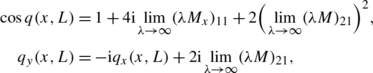
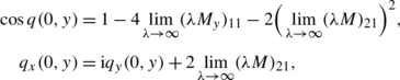
The proof of properties (i)–(iv) follows from the discussion in Sect. 2.2. In particular, property (iii) follows from the asymptotic behaviour at λ→0, which can be derived by analyzing equations (2.2)–(2.3) (see Pelloni 2009), and is given by
To prove (v), we note that the function Φ 1(x,λ) given by (2.17) is the unique solution of the ODE

Furthermore, Φ 3(x,λ) given by (2.19) is the solution of the same ODE problem, with Q(x,L,λ) replaced by Q(x,0,λ).
Similarly, Φ 2(y,λ) given by (2.18) is the unique solution of the ODE

The spectral analysis of the above ODEs yields the desired result.
Regarding the rigorous derivation of the above results, we note the following: If {q(x,L),q y (x,L)}, {q(x,0),q y (x,0)} and {q(y,0),q x (y,0)} are in \({\bf L}^{1}\), then the Volterra integral equations (3.1), (3.4) and (3.5), respectively, have a unique solution, and hence the spectral functions {a j ,b j }, j=1,…,3, are well defined. Moreover, under the assumption (2.1) the spectral functions belong to \({\bf H}^{1}({\mathbb{R}})\), hence the Riemann–Hilbert problems that determine the inverse maps can be characterised through the solutions of a Fredholm integral equation, see Deift (2000) and Zhou (1989).
3.2 The Riemann–Hilbert Problem
Theorem 3.1
Suppose that a subset of the boundary values {q(x,L),q y (x,L)}, {q(x,0),q y (x,0)}, 0<x<∞, and {q(y,0),q x (y,0)}, 0<y<L, satisfying (2.1), are prescribed as boundary conditions. Suppose that these prescribed boundary conditions are such that the global relations (2.22a), (2.22b) can be used to characterise the remaining boundary values.
Define the spectral functions {a j ,b j }, j=1,…,3, by definitions (3.1)–(3.3). Assume that the possible zeros \(\{{\lambda }_{j}\}_{j=1}^{N_{1}}\) of a 1(λ) and \(\{\zeta_{j}\}_{j=1}^{N_{3}}\) of a 3(λ) are as in assumption (2.29).
Define M(x,y,λ) as the solution of the following 2×2 matrix Riemann–Hilbert problem:
-
The function M(x,y,λ) is a sectionally meromorphic function of λ away from ℝ∪iℝ.
-
The possible poles of the second column of M occur at λ=ζ j , j=1,…,N 3, in the first quadrant and at λ=λ j , j=1,…,N 1, in the second quadrant of the complex λ plane.
The possible poles of the first column of M occur at λ=−λ j (j=1,…,N 1) and λ=−ζ j (j=1,…,N 3).
The associated residue conditions satisfy the relations (2.32).
-
\(M=I+\mathrm{O} (\frac{1}{{\lambda }})\) as λ→∞, and
$$M_-(x,y,{\lambda })=M_+(x,y,{\lambda })J(x,y,{\lambda }),\quad {\lambda }\in {\mathbb{R}}\cup \mathrm{i}{\mathbb{R}}, $$where M=M + for λ in the first or third quadrant, and M=M − for λ in the second or fourth quadrant of the complex λ plane, and J is defined in terms of {a j ,b j } by (2.26).
Then M exists and is unique, provided that the \({\bf H}^{1}\) norm of the spectral functions is sufficiently small.
Define q(x,y) is terms of M(x,y,λ) by


Then q(x,y) solves (1.1). Furthermore, q(x,y) evaluated at the boundary, yields the functions used for the computation of the spectral functions.
Proof
Under the assumptions (2.1), the spectral functions are in \({\bf H}^{1}\).
In the case when a 1(λ) and a 3(λ) have no zeros, the Riemann–Hilbert problem is regular and it is equivalent to a Fredholm integral equation. However, we have not been able to establish a vanishing lemma, hence we require a small norm assumption for solvability.
If a 1(λ) and a 3(λ) have zeros, the singular RH problem can be mapped to a regular one coupled with a system of algebraic equations (Fokas and Its 1996). Moreover, it follows from standard arguments, using the dressing method (Zakharov and Shabat 1974, 1979), that if M solves the above RH problem and q(x,y) is defined by (3.7)–(3.8), then q(x,y) solves (1.1). The proof that q evaluated at the boundary yields the functions used for the computation of the spectral functions follows arguments similar to the ones used in Fokas et al. (2005). □
4 Linearisable Boundary Conditions
We now concentrate on the particular boundary conditions (1.3). We note that these boundary conditions are symmetric with respect to the line \(y=\frac{L}{2}\). Hence, if q(x,y) is a solution, so is q(x,L−y). Assuming that the solution is unique, we can conclude that
These boundary conditions are not compatible at the corners of the domain, and therefore introduce a discontinuity at each corner. It turns out that these discontinuities imply that if q(x,y) is the solution of the resulting boundary value problem, then the function q y (x,0)=−q y (x,L) is not integrable near x=0. Similarly, q x (0,y) is not integrable near y=0 and y=L. Hence we cannot guarantee that the results of Propositions 3.1–3.3 hold. In particular, the spectral functions as given by (2.17)–(2.19) and the resulting Riemann–Hilbert problem are not well defined.
To overcome this lack of regularity, we will employ a gauge transformation to define a modified Lax pair. This transformation is motivated by the recent analysis of the linearised problem (Ashton and Fokas 2012), which we summarise in Appendix. For the linear case, it can be shown that the behaviour of the boundary function q y (x,0) as x→0 is given by \(q_{y}(x,0)\sim\frac{2d}{\pi x}\). The contribution of this term can be eliminated by an appropriate gauge transformation. The advantage of the new Lax pair we define below by adapting the linear gauge transformation to the nonlinear setting, is that the spectral functions and the Riemann–Hilbert problem are well defined, indicating that in the nonlinear case, as in the linear, the singular behaviour introduced by the terms q y (x,0) and q x (0,y) is eliminated.
4.1 A New Lax Pair
The linearised version of the elliptic sine-Gordon equation, namely the modified Helmholtz equation, with the boundary conditions (1.3), is discussed in Appendix, where we show how, by incorporating appropriately in the differential form associated with the linear equation the term
the spectral problem is regularised.
Motivated by the linear analysis, we now introduce a new eigenfunction Φ via the gauge transformation
where Ψ denotes the solution of the Lax pair (2.2)–(2.3) and κ(x,y) is given by (4.2). Note that
The transformation matrix g(x,y) has unit determinant, and is chosen to satisfy the property
Let the function Φ satisfy the Lax pair


with


We now use the eigenfunctions determined by the Lax pair (4.4)–(4.5) to define new spectral functions. Namely, in analogy with (2.17)–(2.19), we define


Note that V 1 does not involve q y (x,y), and V 2 does not involve q x (x,y), the terms, respectively, responsible, at least in the linear case, for the non-integrable behaviour.
Note also that, since the symmetry relation (2.20) holds for V 1, V 2 in place of Q, we can represent the matrices φ i in the form

and set
The rest of the general construction of Sects. 2.3–3.2 is formally valid with the spectral functions a j (λ), b j (λ), j=1,2,3 as defined by (4.12), except for the statement (i)–(iii) and (v) of Propositions 3.1–3.3.
4.1.1 Symmetry Conditions
Given the boundary conditions (1.3), (4.8)–(4.10) are written explicitly as follows:


Using that κ(x,0)=−κ(x,L), we can immediately conclude that
where A i , B 1, a i , b i are as in (4.11)–(4.12).
In (4.13) and (4.15), the only dependence on λ is through Ω(λ). Thus, since \(\varOmega(-\frac{1}{\lambda})=\varOmega(\lambda)\), it follows that the vector functions (A 1,B 1) and (A 3,B 3) satisfy the same symmetry properties. Hence,
It turns out that the vector function (A 2,B 2) also satisfies a certain symmetry condition, as stated in the following proposition.
Proposition 4.1
Let q x (0,y) be a sufficiently smooth function. Then the vector solution of the linear Volterra integral equation (4.14) satisfies the following symmetry conditions:

where the function F(λ) is defined by
Proof
Define a function ϕ 2(y,λ) by
where φ 2 is defined by (4.14). It follows that ϕ 2 satisfies the ODE

where
We seek a nonsingular matrix R(λ), independent of y, such that
It can be verified that such a matrix is given by
where F is defined by (4.19).
Replacing in (4.21) λ by \(\frac{1}{{\lambda }}\), and using (4.23), we find the following equation:
hence
where C is a y-independent matrix. Using the second of (4.21), it follows that C=R −1, and therefore
This equation and (4.20) imply
The first column vector of this equation implies (4.18). □
Remark 4.1
Recalling that a 2(λ)=A 2(0,λ), and b 2(λ)=B 2(0,λ), equations (4.18) immediately imply the following important relations:

In summary, the basic equations characterizing the spectral functions are:
- (a)
- (b)
-
(c)
the conditions of unit determinant.
In the next lemma, we collect some important consequences of these conditions. For simplicity, we will use the notations
Lemma 4.1
The spectral functions satisfy the following relations:


where the function G(λ) is defined by

Proof
Equation (4.27) is just the condition of unit determinant.
Using the symmetry condition (4.16) to eliminate a 1 and b 1 from the global relations (2.22a), (2.22b), we find


Equations (4.31a), (4.31b) together with the equations obtained by letting λ→−λ in (4.31a), (4.31b) are four equations which can be solved for the four functions \(\{a_{2}, b_{2}, \hat{a}_{2}, \hat{b}_{2}\}\) with the result that


This proves (4.29).
Replacing λ by −1/λ in (4.31a), (4.31b) and using the symmetry (4.17), we find


Consider the two equations (4.33a), (4.33b) together with the two equations obtained by letting λ→−λ in (4.33a), (4.33b). We can eliminate \(a_{2} (\pm\frac {1}{\lambda} )\) and \(b_{2} (\pm\frac{1}{\lambda} )\) from these four equations by using the symmetry relations (4.26) as well as the symmetry relations obtained by letting λ→−λ in (4.26). The resulting four equations can then be solved for the four functions \(\{a_{2}, b_{2}, \hat{a}_{2}, \hat{b}_{2}\}\) with the result that


Comparing (4.32a) with (4.34a), we find (4.28). □
The functions a 3(λ) and b 3(λ) are defined by (4.12) only for λ in the upper half-plane. However, (4.29) implies that a 3(λ) and b 3(λ) can be analytically extended to the whole complex plane. Indeed, (4.29) provides the analytic continuation of a 3(λ) into ℂ−:

Similarly, (4.29) with λ replaced with −λ provides the analytic continuation of b 3(λ) into ℂ−:

Adopting these extended definitions of a 3(λ) and b 3(λ), analytic continuation implies that the relations (4.27)–(4.29) and the global relations (4.31a), (4.31b) are valid in the whole complex plane.
Proposition 4.2
The spectral functions satisfy the equations


as well as the global relations


where the known function G(λ) is given by (4.30).
5 Spectral Theory in the Linearisable Case
In Appendix we give the solution of the linear case. In this case, the dependence on the unknown spectral function B(λ) is resolved by mapping the basic Riemann–Hilbert problem to an equivalent but simpler one. To define this mapping, in the linear case, it is convenient to employ the two equations (A.19) and (A.20).
For the nonlinear problem, we will use the following equations, which provide the nonlinear analogues of (A.19) and (A.20):
and
where the unknown function h(λ) is defined by
and the known function G(λ) is defined by (4.30). Note that from the above properties it follows that \(\frac{b_{3}(-{\lambda })}{a_{3}({\lambda })}\) is well defined at the zeros of the function h(λ). Moreover, in the linear limit,
and (5.1) and (5.2) become (A.19) and (A.20).
Equations (5.1) and (5.2) are a direct consequence of (4.37)–(4.39). Indeed,

which is equivalent to (5.1) (in the first and second equations above we have used (4.38) and (4.37), respectively). Furthermore,
which, using G(−λ)=−G(λ), becomes (5.2) (in the first and second equations above we have used the relation (4.39) and (5.1) with λ replaced by −λ).
The Properties of the Functions G(λ) and h(λ)
We give a summary of some of the properties of the function G(λ) given by (4.30) and of the unknown function h given by (5.3).
The set of poles of G(λ), denoted by P G ⊂ℂ, is given by

Note that G(λ) has no poles at λ=±i since the term eωL−1 vanishes at these points.
Proposition 5.1
The following statements hold:
-
(a)
G(λ) admits the symmetries G(λ)=−G(−λ)=−G(1/λ), λ∈ℂ.
-
(b)
G(λ) has essential singularities at ∞ and at 0 and a countable number of simple poles on the imaginary axis accumulating at ±i∞ and at 0. G(λ) has no other singularities.
-
(c)
Each of the functions 1±G(λ) has a countable number of zeros. All these zeros lie on the imaginary axis and they accumulate only at ±i∞ and at 0.
-
(d)
The set of zeros of the function 1−G(λ) is the disjoint union of the set of zeros of a 3(λ)−b 3(λ) and the set of zeros of a 3(−λ)+b 3(−λ).
-
(e)
The set of zeros of the function 1+G(λ) is the disjoint union of the set of zeros of a 3(λ)+b 3(λ) and the set of zeros of a 3(−λ)+b 3(−λ).
-
(f)
The set of zeros of the function 1−G 2(λ) is the disjoint union of the set of zeros of h(λ) and the set of zeros of h(−λ).
-
(g)
The function h(λ) has a double pole at each point in the set P G ∩ℂ−. The function h(−λ) has a double pole at each point in the set P G ∩ℂ+. The functions h(λ) and h(−λ) do not have any other poles.
Proof
The proof of (a) follows from the definition (4.30). The proof of (b) follows from the same definition and from (5.4).
In order to prove (c), we note that the function G is purely real for λ∈iℝ:
As λ I increases from 0 to +∞, the argument \(L\frac{{\lambda }_{I}^{2} -1}{4{\lambda }_{I}}\) increases from −∞ to ∞. It follows that each of the functions 1+G(λ) and 1−G(λ) has an infinite number of zeros on the imaginary axis, see Fig. 4. More precisely, if ip 1 and ip 2 are two consecutive poles of G on the positive imaginary axis, then, unless p 1<1<p 2, there is exactly one zero of 1−G(λ) and one zero of 1+G(λ) belonging to the interval (ip 1,ip 2). If p 1<1<p 2, then there are no zeros of 1+G(λ) in the interval (ip 1,ip 2) and there are two (counted with multiplicity) or no zeros of 1−G(λ) in this interval depending on whether \(G(\mathrm{i}) = \frac{L}{2}\tan(d/2)\) is ≤1 or >1. Since the poles of G(λ) accumulate at 0 and at ±i∞, the same is true for the zeros of 1±G(λ). This proves (c).

(a) The graph of G(λ) for λ on the imaginary axis when L=10 and d=1. (b) The corresponding picture of the poles of G(λ) and the zeros of G(λ)±1. The poles and zeros accumulate at the origin and at infinity
Taking the sum and difference of (4.37) and (4.38) we find

It follows that
Equation (5.5) implies that either a 3−b 3 or \(\hat {a}_{3} + \hat{b}_{3}\) vanishes whenever 1−G=0. Since all zeros of 1−G are simple, the functions a 3−b 3 and \(\hat{a}_{3} + \hat {b}_{3}\) cannot simultaneously vanish at one of these zeros. In order to prove (d), it only remains to show that 1−G vanishes whenever a 3−b 3 or \(\hat{a}_{3} + \hat{b}_{3}\) does. Equation (5.5) suggests that this is true; however, it is conceivable that a zero (pole) of a 3−b 3 could coincide with a pole (zero) of \(\hat {a}_{3} + \hat{b}_{3}\) in such a way that the product \((a_{3} - b_{3})(\hat {a}_{3} + \hat{b}_{3}) = 1 - G\) remains nonzero. We show now that this cannot occur.
Suppose λ 0 is a zero of a 3(λ)−b 3(λ). The unit determinant condition (4.37) implies that a 3(λ) and b 3(λ) cannot simultaneously vanish. Thus,
The global relations (4.40a), (4.40b) yield

Using these equations to eliminate b 2(λ) and b 2(−λ) from the determinant condition
we find

If λ 0 is a zero of a 3(λ)−b 3(λ), then, by (4.17), so is −1/λ 0, and hence we also have

On the other hand, the symmetry condition (4.26) for a 2(λ) implies that

Indeed, if we use (4.26) to eliminate a 2(±1/λ) from the left-hand side of (5.10) and then simplify, we find the right-hand side of (5.10). Evaluating (5.10) at λ=λ 0 and using (5.8) and (5.9) to eliminate a 2(−1/λ 0) and a 2(−λ 0) from the resulting equation, we find

In view of (5.7), (5.8), and (5.11), the symmetry equation (4.26) for a 2(λ) evaluated at λ=λ 0 reduces to
This shows that 1−G(λ)=0 whenever a 3(λ)−b 3(λ)=0. A similar argument shows that 1−G(λ)=0 also whenever a 3(−λ)+b 3(−λ)=0. This proves (d). The proof of (e) is similar.
The statement (f) follows from (d) and (e) since h=(a 3−b 3)(a 3+b 3).
Since h(λ) is analytic in ℂ+ and h(λ) does not vanish at any point λ∈P G by (f), (5.6) implies that h(−λ) has a double pole at each point in the set P G ∩ℂ+. This proves (g). □
5.1 An Equivalent Riemann–Hilbert Problem
Using the relations (4.16) and (4.32a), the jump matrices (2.26) become

and
Let M(x,y,λ) be defined by (2.24) with Ψ j replaced with Φ j , j=1,2,3. Let D j denote the jth quadrant of the complex plane,
and let M j denote the restriction of M to D j .
The jump matrices (5.12) involve the unknown spectral functions b 2(λ),a 3(λ), and b 3(λ). We therefore seek matrices A j (x,y,λ), j=1,…,4, defined for λ∈D j , such that the functions \(\{\tilde{M}_{j}(x,y,{\lambda })\}_{1}^{4}\) by
satisfy a modified Riemann–Hilbert problem whose jump matrices involve only known functions. We would like A j to be bounded and analytic (or at least meromorphic) for λ∈D j .
The requirement that A j is bounded in the jth quadrant implies that A 1 and A 2 are upper triangular, while A 3 and A 4 are lower triangular. The requirement that A j has unit determinant implies that the diagonal elements of A j are d j and \(\frac{1}{d_{j}}\). The (2,2) components of (5.18) imply that
On the other hand, the four exponential factors

are bounded in the first, second, third and fourth quadrant of the complex λ-plane, respectively.
This suggests choosing the matrices A j in the following form:


where α j (λ), j=1,…,4, is a scalar valued function of λ∈D j .
Substituting (5.13) into the jump relations
we find the equations
provided that the matrices \(\tilde{J}^{0}\), \(\tilde{J}^{\pi/2}\), \(\tilde{J}^{3\pi/2}\) satisfy the following equations:
We analyse the first of (5.18). The (2,2) element of this equation is satisfied identically and the (1,1) element is a consequence of the (1,2) and (2,1) elements, as well as of the requirement that all matrices in (5.18) have unit determinant. Denoting the (1,2) and (2,1) components of \(\tilde{J}^{0}\) by \({\rm e}^{-\theta(x,y,\lambda)}\tilde{U}^{0}({\lambda })\) and \({\rm e}^{\theta(x,y,\lambda)}{\rm e}^{-\omega({\lambda })L}\tilde{V}^{0}({\lambda })\), respectively, we find that the (1,2) and (2,1) elements of the first of equations (5.18) yield
and
Comparing (5.19) with the identity (5.1) we find that a simple choice for the function α 1 (and hence for \(\tilde{U}^{0}\)) is \(\alpha_{1}({\lambda })=\frac{b_{3}({\lambda })}{a_{3}({\lambda })h({\lambda })}\) and \(\tilde{U}^{0}({\lambda })=-\frac{G({\lambda })}{h({\lambda })}\). Note that these functions are well defined on ℝ since h does not have any real zero. However, with these choices the functions α 1(λ) and \(\tilde{U}^{0}({\lambda })\) have (i) poles at the (unknown) zeros of h(λ) along the imaginary axis and (ii) poles at the (known) poles of G(λ) along the imaginary axis. To ensure that the poles in (i) are removable singularities we define the function \(\tilde{G}({\lambda })\) as follows:
This function takes values 1 and −1 exactly where G(λ) does. Indeed, if h(λ)=0, then a 3(λ)=±b 3(λ) and correspondingly, in view of (5.5), \(G({\lambda })=\tilde{G}({\lambda })=\pm1\).
The above discussion suggests that a suitable choice for the functions α 1(λ) and \(\tilde{U}^{0}({\lambda })\) is
Similarly, (5.20) suggests
We next analyse the second of equations (5.18). The (1,2) element of this equation yields
where \(\tilde{U}^{\pi/2}({\lambda }){\rm e}^{-\theta(x,y,\lambda)}\) denotes the (1,2) component of \(\tilde{J}^{\pi/2}\). Using the identity (5.2), we find
This suggests that we define
A similar analysis of the third of equations (5.18) yields
where \(V^{3\pi/2}({\lambda }){\rm e}^{\theta(x,y,\lambda)}\) denotes the (2,1) component of \(\tilde{J}^{\frac{3\pi}{2}}\). Note that the relations α 2(λ)=α 4(−λ) and α 3(λ)=α 1(−λ) are consistent with the symmetry (2.20).
We define the matrices A j , j=1,…,4, by (5.15a)–(5.15d) and (5.22)–(5.25). Henceforth, we assume that (x,y) lies in the interior of the semistrip (1.2) so that x>0 and 0<y<L. Then the jth exponential factor in (5.14) has exponential decay as λ→∞ and λ→0 for \({\lambda }\in\bar{I}_{j}\). Thus, although the analysis of the linear problem suggests that the spectral functions a j (λ),b j (λ) could have some minor growth as λ→∞ and λ→0 caused by the jumps in the boundary data at the corners of the semistrip (in the linear case this growth is logarithmic, see Appendix), this ensures that the A j ’s are bounded as λ→∞ and as λ→0 in the corresponding domains D j .
In fact, since the A j ’s have removable singularities at the zeros of the function h(λ) along the imaginary axis, the only remaining difficulty is that the A j ’s have singularities at the known poles of G(λ). To deal with these singularities, we add small indentations to the jump contour along the imaginary axis so that it passes to the right of the poles of G. Thus, instead of the four quadrants D j of the complex plane, we consider the deformed domains \(\tilde{D}_{j}\) defined in such a way that all λ∈P G ∩ℂ+ lie in \(\tilde{D}_{1}\) and all λ∈P G ∩ℂ− lie in \(\tilde {D}_{3}\), see Fig. 5.

The contour for the modified Riemann–Hilbert problem satisfied by \(\tilde{M}\). The contour has small indentations bypassing the poles of G(λ)
We next determine the residue conditions at these poles. Let λ ∗∈P G ∩ℂ+ be a pole of α 1 in \(\tilde{D}_{1}\). In what follows, we use the notation M(x,y,λ)=([M(x,y,λ)]1,[M(x,y,λ)]2) to denote the first and second column vector of a given matrix M(x,y,λ). Then the relation \(\tilde{M}_{1} = M_{1} A_{1}\) implies that

Taking the residue of the second of these equations at λ ∗, we find

where the residue of G(λ) at λ ∗ is known from the definition (4.30) whereas the number h(λ ∗) remains unknown.
Similarly, the relation \(\tilde{M}_{3} = M_{3} A_{3}\) implies that

Taking the residue of the first of these equations at λ ∗∈P G ∩ℂ−, we find

In summary, we have derived the following result.
Theorem 5.1
The RH problem defined in Theorem 3.1 and characterised by the jump matrices {J π/2,J 3π/2,J 0,J π} defined in (5.12), can be mapped to a new RH problem with the following jump matrices:

where the known function G(λ) is defined in (4.30). This is achieved by using the matrices (5.15a)–(5.15d), with

where the functions h(λ) and \(\tilde{G}({\lambda })\) are defined by (5.3) and (5.21), respectively. The solution \(\tilde {M}\) of the new RH problem is a sectionally meromorphic function with simple poles at each point in the set P G given in (5.4). At these points the following residue conditions are valid:


The solution q(x,y), x>0, 0<y<L, of the boundary value problem determined by the boundary conditions (1.3) is given by


Proof
We only need to show how to represent the solution q(x,y) of the boundary value problem in terms of the solution of the RH problem characterised by the jump matrices given by (5.26). Recall that if M(x,y,λ) denotes the solution of the RH problem defined in Theorem 3.1 then q(x,y) is defined in terms of M by (3.7)–(3.8). Using \(\tilde{M}_{j}=A_{j}M_{j}\) in the jth quadrant, j=1,…,4, by choosing λ in the first quadrant we obtain

Since \({\rm e}^{-\theta(x,y,\lambda)}\) decays exponentially as λ→∞ in the first quadrant, the term involving the unknown coefficient α 1 does not contribute to the limit and we find (5.30)–(5.31). □
6 Conclusions and Open Problems
We have analysed the elliptic sine-Gordon equation in a semistrip for general boundary data (Sects. 2 and 3) and in the particular case of a linearisable boundary value problem (Sects. 4 and 5). The linearisable problem has the novelty that the function q y (x,0) possesses a non-integrable singularity as x→0 while the function q x (0,y) possesses a non-integrable singularity as y→0. Motivated by the recent solution of an analogous problem for the modified Helmholtz equation presented in Ashton and Fokas (2012), we have been able to bypass this problem by employing a suitable gauge transformation. Furthermore, we have shown that the RH problem characterizing the solution q(x,y) can be mapped to a modified RH problem whose “jump matrix” is determined only by the width L of the semistrip and the given constant value d of the boundary condition prescribed at x=0 (see Theorem 5.1). However, the modified RH problem also includes residue conditions at the points λ∈P G , where the set P G consists of a countable number of points on the imaginary axis. The formulation of these residue conditions requires the knowledge of h(λ) for λ∈P G , where h(λ) is an unknown meromorphic function defined in terms of the spectral functions. It remains an open problem to characterise the values of h(λ) for λ∈P G in terms of L and d alone; progress in this direction is likely to rely on the analyticity properties of h(λ) as well as on relations derived from the symmetry properties of the spectral functions, such as the relation (5.6), and the known structure of the poles of h.
References
Antipov, Y., Fokas, A.S.: The modified Helmholtz equation in a semi-strip. Math. Proc. Camb. Philos. Soc. 138, 339–365 (2005)
Ashton, A., Fokas, A.S.: Elliptic boundary value problems in convex polygons with low regularity boundary data via the unified method (2012, under review)
ben-Avraham, D., Fokas, A.S.: The modified Helmholtz equation in a triangular domain and an application to diffusion-limited coalescence. Phys. Rev. E 64, 016114 (2001)
Bona, J.L., Fokas, A.S.: Initial-Boundary-Value problems for linear and integrable nonlinear dispersive partial differential equations. Nonlinearity 21(10), T195–T203 (2008)
Borisov, A.B., Kiseliev, V.V.: Inverse problems for an elliptic sine-Gordon equation with an asymptotic behaviour of the cnoidal type. Inverse Probl. 5, 959–982 (1989)
Boutet de Monvel, A., Fokas, A.S., Shepelsky, D.: The analysis of the global relation for the nonlinear Schrödinger equation on the half-line. Lett. Math. Phys. 65, 199–212 (2003)
Boutet de Monvel, A., Fokas, A.S., Shepelsky, D.: The modified KdV equation on the half-line. J. Inst. Math. Jussieu 3, 139–164 (2004)
Crowdy, D., Fokas, A.S.: Explicit integral solutions for the plane elastostatic semi-strip. Proc. R. Soc. Lond. A 460, 1285–1309 (2004)
Dassios, G., Fokas, A.S.: The basic elliptic equations in an equilateral triangle. Proc. R. Soc. Lond. A 461, 2721–2748 (2005)
Deift, P.: Orthogonal Polynomials and Random Matrices: A Riemann–Hilbert Approach. American Mathematical Society, Providence (2000)
Dujardin, G.M.: Asymptotics of linear initial boundary value problems with periodic boundary data on the half-line and finite intervals. Proc. R. Soc. Lond. A 465, 3341–3360 (2009)
Flyer, N., Fokas, A.S.: A hybrid analytical numerical method for solving evolution partial differential equations. I. The half-line. Proc. R. Soc. 464, 1823–1849 (2008)
Fokas, A.S.: A unified transform method for solving linear and certain nonlinear PDE’s. Proc. R. Soc. Ser. A 453, 1411–1443 (1997)
Fokas, A.S.: On the integrability of linear and nonlinear partial differential equations. J. Math. Phys. 41, 4188–4238 (2000)
Fokas, A.S.: Two dimensional linear PDE’s in a convex polygon. Proc. R. Soc. Lond. A 457, 371–393 (2001)
Fokas, A.S.: Nonlinear evolution equations on the half line. Commun. Math. Phys. 230, 1–39 (2002a)
Fokas, A.S.: A new transform method for evolution PDEs. IMA J. Appl. Math. 67, 1–32 (2002b)
Fokas, A.S.: Linearizable initial boundary value problems for the sine-Gordon equation on the half line. Nonlinearity 17, 1521–1534 (2004)
Fokas, A.S.: The generalized Dirichlet-to-Neumann map for certain nonlinear evolution PDEs. Commun. Pure Appl. Math. LVIII, 639–670 (2005)
Fokas, A.S.: A Unified Approach to Boundary Value Problems. CBMS-NSF Regional Conference Series in Applied Mathematics. SIAM, Philadelphia (2008)
Fokas, A.S., Its, A.R.: The linearization of the initial-boundary value problem of the nonlinear Schrödinger equation. SIAM J. Math. Anal. 27, 738–764 (1996)
Fokas, A.S., Its, A.R.: The nonlinear Schrödinger equation on the interval. J. Phys. A 37, 6091–6114 (2004)
Fokas, A.S., Lenells, J.: Explicit soliton asymptotics for the Korteweg-de-Vries equation on the half-line. Nonlinearity 23, 937 (2010)
Fokas, A.S., Lenells, J.: The unified method: I. Non-linearizable problems on the half-line. J. Phys. A: Math. Theor. 45, 195201 (2012)
Fokas, A.S., Menyuk, C.: Integrability and similarity in transient stimulated Raman scattering. J. Nonlinear Sci. 9, 1–31 (1999)
Fokas, A.S., Pelloni, B.: A transform method for linear evolution PDEs on a finite interval. IMA J. Appl. Math. 70, 1–24 (2005)
Fokas, A.S., Spence, E.A.: Novel analytical and numerical methods for elliptic boundary value problems. In: Highly Oscillatory Problems. Cambridge University Press, Cambridge (2009)
Fokas, A.S., Zyskin, M.: The fundamental differential form and boundary value problems. Q. J. Mech. Appl. Math. 55, 457–479 (2002)
Fokas, A.S., Its, A.R., Sung, L.Y.: The nonlinear Schrödinger equation on the half-line. Nonlinearity 18, 1771–1822 (2005)
Gutshabash, E.S., Lipovskii, V.D.: Boundary value problem for the two-dimensional elliptic sine-Gordon equation and its applications to the theory of the stationary Josephson effect. J. Math. Sci. 68, 197–201 (1994)
Lax, P.D.: Integrals of nonlinear equations of evolution and solitary waves. Commun. Pure Appl. Math. 21, 467–490 (1968)
Lenells, J.: Boundary value problems for the stationary axisymmetric Einstein equations: a disk rotating around a black hole. Commun. Math. Phys. 304, 585–635 (2011)
Lenells, J., Fokas, A.S.: An integrable generalisation of the nonlinear Schrödinger equation on the half-line and solitons. Inverse Probl. 25 (2009)
Lenells, J., Fokas, A.S.: Boundary value problems for the stationary axisymmetric Einstein equations: a rotating disk. Nonlinearity 24, 177 (2011)
Lenells, J., Fokas, A.S.: The unified method: II. NLS on the half-line with t-periodic boundary conditions. J. Phys. A Math. Theor. 45, 195202 (2012a)
Lenells, J., Fokas, A.S.: The unified method: III. Non-linearizable problems on the interval. J. Phys. A, Math. Theor. 45, 195203 (2012b)
Lipovskii, V.D., Nikulichev, S.S.: Vestn. LGU Ser. Fiz. Khim. 4, 61–134 (1988)
Pelloni, B.: Well posed boundary value problems for linear evolution equations in finite intervals. Math. Proc. Camb. Philos. Soc. 136, 361–382 (2004)
Pelloni, B.: The spectral representation of two-point boundary value problems for linear evolution equations. Proc. R. Soc. A 461, 2965–2984 (2005a)
Pelloni, B.: The asymptotic behaviour of the solution of boundary value problems for the sine-Gordon equation on a finite interval. J. Nonlinear Math. Phys. 12(4), 518–529 (2005b)
Pelloni, B.: Spectral analysis of the elliptic sine-Gordon equation in the quarter plane. Theor. Math. Phys. 160(1), 1031–1041 (2009)
Pelloni, B., Pinotsis, D.A.: The Klein-Gordon equation on the half line: a Riemann–Hilbert approach. J. Nonlinear Math. Phys. 15, 334–344 (2008)
Pelloni, B., Pinotsis, D.A.: The elliptic sine-Gordon equation in a half plane. Nonlinearity 23, 77–88 (2010)
Smitheman, S.A., Spence, E.A., Fokas, A.S.: A spectral collocation method for the Laplace and modified Helmholtz equations in a convex polygon. IMA J. Numer. Anal. 30, 1184–1205 (2010)
Spence, E.A., Fokas, A.S.: A new transform method I: domain dependent fundamental solutions and integral representations. Proc. R. Soc. A 466, 2259–2281 (2010a)
Spence, E.A., Fokas, A.S.: A new transform method II: the global relation, and boundary value problems in polar co-ordinates. Proc. R. Soc. A 466, 2283–2307 (2010b)
Treharne, P.A., Fokas, A.S.: The generalized Dirichlet to Neumann map for the KdV equation on the half-line. J. Nonlinear Sci. 18, 191–217 (2008)
Zakharov, V.E., Shabat, A.B.: A scheme for integrating the nonlinear equations of numerical physics by the method of the inverse scattering problem I. Funct. Anal. Appl. 8, 226–235 (1974)
Zakharov, V.E., Shabat, A.B.: A scheme for integrating the nonlinear equations of numerical physics by the method of the inverse scattering problem II. Funct. Anal. Appl. 13, 166–174 (1979)
Zhou, X.: The Riemann–Hilbert problem and inverse scattering. SIAM J. Math. Anal. 20(4), 966–986 (1989)
Acknowledgements
This research was partially supported by EPSRC grant EP/E022960/1. ASF would like to express his gratitude to the Guggenheim Foundation, USA.
Author information
Authors and Affiliations
Corresponding author
Additional information
Communicated by P. Newton.
Appendix: The Modified Helmholtz Equation
Appendix: The Modified Helmholtz Equation
The basic differential form associated with the modified Helmholtz equation
is given by
where Ω(λ) and ω(λ) are defined in (2.4). Indeed, it can be verified that
Suppose that u y (x,y) has non-integrable singularities at (0,0) and (0,L). In order to eliminate these singularities we consider the differential form
and choose κ in such a way that the term u y cancels. Noting that
we choose κ as in (4.2):
Then

where we have used
We define Φ j (x,y,λ), j=1,3,4, as the solutions of the equation
with
see Fig. 6.

The contours of integration used to define Φ j (x,y,λ), j=1,3,4
The difference of any two of the above functions equals \({\rm e}^{\varOmega x+\omega y}\rho({\lambda })\), where ρ(λ) can be computed by evaluating the difference at any convenient point (x,y). Hence

where
and the above choice for the domains of validity with respect to λ in (A.5) will be justified below.
Equations (A.3) and the first of equations (A.4) imply that
Hence the first and the third of equations (A.6) imply that


In order to compute Φ 4(0,0,λ) we compute Φ 4 along the y-axis from (0,L) to (0,0):

The last integral of this equation is given by

Hence, using this equation, as well as the identity Ω 2+ω 2=1, (A.10) together with the second of equations (A.6) yields

Subtracting the second of equations (A.5) from the sum of the other two equations in (A.5) we find the global relation
1.1 A.1 Example
Let
The expressions in (A.8) and (A.11) simplify as follows:

Note that ω(±i)=0, thus the first term of the right-hand side of (A.14) has removable singularities at ±i.
The overall symmetry u(x,y)=u(x,L−y) implies
Thus the global relation (A.12) becomes
The only dependence of B 3 on λ is through Ω(λ), which remains invariant under the transformation \({\lambda }\to-\frac{1}{{\lambda }}\), thus
The second term of the right-hand side of the first of equations (A.14) involves Ω 2(λ) and ω(λ), which are invariant under the transformation \({\lambda }\to\frac{1}{{\lambda }}\). Thus we find
therefore
In summary, taking into account that B 1=−B 3, it follows that the modified Helmholtz equation in the semistrip, with the boundary conditions (1.3), involves the two unknown spectral functions B 3(λ) and B 2(λ), defined in terms of the two unknown functions f 2(λ) and f 3(λ) by (A.13) and (A.14). These two spectral functions satisfy the global relation (A.16) as well as the symmetry relations (A.17) and (A.18).
In what follows, we will show that the unknown functions B 2 and B 3 yields a zero contribution to the representation of the solution u(x,y). In order to prove this fact, we need the following identities, which are a consequence of (A.16)–(A.18):

Indeed, letting \({\lambda }\to\frac{1}{{\lambda }}\) in the global relation (A.16) we find
Using in the above equation the symmetry relation (A.17) with λ→−λ, as well as the symmetry relation (A.18), we find (A.20). Subtracting (A.20) from the global relation (A.16) we find (A.19). The functions G 1(λ), G 2(λ) have removable singularities at λ=±i.
The functions Φ j (x,y,λ), j=1,3,4, define a Riemann–Hilbert problem with jumps on the real and negative imaginary axis, see Fig. 7.

The contour for the Riemann–Hilbert problem
In order to map this Riemann–Hilbert problem to a problem with known jump conditions, we introduce the functions \(\tilde{\varPhi}_{j}(x,y,{\lambda })\), j=1,3,4, through the following equations:

It is shown in Remark 7.1 at the end of this appendix that the function B 3(λ) has a logarithmic singularity as λ→0 and λ→∞. In particular, assuming that (x,y) lies in the interior of the semistrip (1.2) so that x>0 and 0<y<L, it follows that \({\rm e}^{\theta(x,y,{\lambda })}B_{3}(-{\lambda })\) and \({\rm e}^{\theta(x,y,{\lambda })}{\rm e}^{-\omega({\lambda })L}B_{3}(-{\lambda })\) are bounded and analytic for λ in the third and fourth quadrant of the λ plane, respectively.
Using the definitions (A.21) in (A.5), we find

Equations (A.19) and (A.20) imply that the jump conditions appearing in (A.22) can be expressed in terms of the known functions G 1 and G 2.
Equation (A.3) implies that the function Φ satisfies the equation
This equation suggests that
This estimate can be verified using (A.7) and integration by parts. The first of equations (A.21) shows that \(\tilde{\varPhi}_{1}\) satisfies the same estimate (A.24). Solving the Riemann–Hilbert problem with the jump conditions (A.22) and the estimate (A.24) (for \(\tilde{\varPhi}_{1}\)) we find

Hence taking the limit of this equation as λ→0 we find

On the other hand, (A.23) implies that
Noting that \(\varPhi=\tilde{\varPhi}\) for λ∈ℂ+, we find

In summary, the solution of the BVP obtained by taking the linear limit of (1.1) and (1.3) is given by (A.27) where G 1 and G 2 are defined by (A.19) and (A.20).
In what follows we verify that the function u(x,y) defined by (A.27) satisfies the given boundary conditions.
1.1.1 A.1.1 u(x,0)=0
Evaluating (A.27) at y=0 we find

The integrands of the second and third integrals of the right-hand side of (A.28) are bounded and analytic in the fourth quadrant of the complex λ plane. In order to map the first integral to an integral whose integrand is also bounded and analytic in the fourth quadrant, we replace in the first integral λ by \(-\frac{1}{{\lambda }}\):
Then combining this term with the second integral we find an integral involving
Hence (A.28) becomes
By Jordan’s lemma, the right-hand side of this equation vanishes (λ=−i is a removable singularity) and hence u(x,0)=0.
1.1.2 A.1.2 u(x,L)=0
Evaluating (A.27) at y=L, we find

The integrands of the first and third integrals of the right-hand side of (A.29) are bounded and analytic in the third quadrant of the complex λ plane. In order to map the second integral to an integral whose integrand is also bounded and analytic in the third quadrant, we replace in the second integral λ by \(-\frac{1}{{\lambda }}\):
Then combining this term with the first integral we find an integral involving \((1+{\rm e}^{\omega({\lambda })L})G_{1}\). Hence (A.29) becomes
By Jordan’s lemma, the right-hand side of this equation vanishes; hence u(x,L)=0.
1.1.3 A.1.3 u(0,y)=d
Evaluating (A.27) at x=0, we find

The first and second terms of the integrand of the third integral on the right-hand side are analytic in the third and fourth quadrant of the λ complex plane, respectively. Before considering these terms separately, in order to take care of the singularity at λ=−i in the denominator, we deform the contour of integration of the third integral to the curve L depicted in Fig. 8.

The contour for the Riemann–Hilbert problem
Rewriting the term \(\frac{{\rm e}^{\omega({\lambda })L}-1}{{\rm e}^{\omega({\lambda })L}+1}\) in the first and second integrals on the right-hand side of (A.30) in the form, respectively,
(A.30) becomes

Jordan’s lemma implies that the first integral in the right-hand side of (A.31) vanishes. Furthermore, the integrand of the third integral in the right-hand side of (A.31) remains invariant under the transformation \({\lambda }\to\frac{1}{{\lambda }}\), thus this integral also vanishes. The second integral on the right-hand side of (A.31) has a pole at λ=−i with residue −1. Hence, u(0,y)=d.
Remark 6.1
(The asymptotics of B 3(λ) as λ→0 and λ→∞)
Using (A.27), it is possible to show (see Ashton and Fokas 2012) that

Hence, the definition (A.13) of B 3(λ) implies that

Integration by parts implies that the first term of the r.h.s. of (A.33) is of O(1) as λ→∞ and λ→0. The second term in the r.h.s. of (A.33) can be computed explicitly,
Hence

In particular,

and

Rights and permissions
About this article
Cite this article
Fokas, A.S., Lenells, J. & Pelloni, B. Boundary Value Problems for the Elliptic Sine-Gordon Equation in a Semi-strip. J Nonlinear Sci 23, 241–282 (2013). https://doi.org/10.1007/s00332-012-9150-5
Received:
Accepted:
Published:
Issue Date:
DOI: https://doi.org/10.1007/s00332-012-9150-5