Probabilistic bisimulation for realistic schedulers

Abstract

Weak distribution bisimilarity is an equivalence notion on probabilistic automata, originally proposed for Markov automata. It has gained some popularity as the coarsest behavioral equivalence enjoying valuable properties like preservation of trace distribution equivalence and compositionality. This holds in the classical context of arbitrary schedulers, but it has been argued that this class of schedulers is unrealistically powerful. This paper studies a strictly coarser notion of bisimilarity, which still enjoys these properties in the context of realistic subclasses of schedulers: Trace distribution equivalence is implied for partial information schedulers, and compositionality is preserved by distributed schedulers. The intersection of the two scheduler classes thus spans a coarser and still reasonable compositional theory of behavioral semantics.

1 Introduction

Compositional theories have been an important technique to deal with complex stochastic systems effectively. Their potential ranges from compositional minimization [4, 7] approaches to component based verification [27, 32]. Due to their expressiveness, Markov automata have attracted many attentions [17, 25, 39], since they were introduced [15]. Markov automata are a compositional behavioral model for continuous time stochastic and non-deterministic systems [14, 15] subsuming interactive Markov chains [29] and probabilistic automata (PAs) [37] (and hence also Markov decision processes and Markov chains).

On Markov automata, weak probabilistic bisimilarity has been introduced as a powerful way for abstracting from internal computation cascades, and this is obtained by relating sub-probability distributions instead of states. In the sequel we call this relation weak distribution bisimulation, and focus on probabilistic automata, arguably the most widespread subclass of Markov automata.

On probabilistic automata, weak distribution bisimilarity is strictly coarser than weak bisimilarity, and is the coarsest congruence preserving trace distribution equivalence [9]. More precisely, it is the coarsest reduction-closed barbed congruence [31] with respect to parallel composition. Decision algorithms for weak distribution bisimilarity have also been proposed [18, 35].

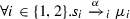
Weak distribution bisimilarity enables us to equate automata such as the ones on the left in Fig. 1, both of which exhibit the execution of action $\alpha$ followed by states $r_1$ and $r_2$ with probability $\frac{1}{2}$ each for an external observer. Specifically, the internal transition of the automaton on the left remains fully transparent. Standard bisimulation notions fail to equate these automata. On the other hand, the automata on the right are not bisimilar even though the situation seems to be identical for an external observer.

Fig. 1

Distinguishing probabilistic automata

The automata on the right of Fig. 1 are to be distinguished, because otherwise compositionality with respect to parallel composition would be broken. However, as observed in [23, 37], the general scheduler in the parallel composition is too powerful: the decision of one component may depend on the history of other components; in Fig. 1, whether $s_4$ or $s_5$ is visited may influence a scheduler decision regarding some other component. This is especially not desired for partially observable systems, such as multi-agent systems or distributed systems [3, 38]. In distributed systems, where components only share the information they gain through explicit communication via observable actions, this behavior is unrealistic. Thus, for practically relevant models, weak distribution bisimilarity is still too fine. The need to distinguish the two automata on the right of Fig. 1 is in fact an unrealistic artifact, and this will motivate our definition of a coarser bisimulation, under which they are equivalent.

In this paper, we present a novel notion of weak bisimilarity on PAs, called late distribution bisimilarity, which is coarser than the existing notions of weak bisimilarity. It equates, for instance, all automata in Fig. 1. As weak distribution bisimilarity is the coarsest notion of equivalence that preserves observable behavior and is closed under parallel composition [9], late distribution bisimilarity cannot satisfy these properties in their entirety. However, as we will show, for a natural class of schedulers, late distribution bisimilarity preserves observable behavior, in the sense that trace distribution equivalence (i) is implied by late distribution bisimilarity, and (ii) is preserved in the context of parallel composition. This for instance implies that time-bounded reachability properties are preserved with respect to parallel composition. The class of schedulers under which these properties are satisfied is the intersection of two well-known scheduler classes, namely partial information schedulers [8] and distributed schedulers [23]. Both classes have been coined as principal means to exclude undesired or unrealistically powerful schedulers. We provide a co-inductive definition for late distribution bisimilarity which echoes these considerations on the automaton level, thereby resulting in a very coarse, yet reasonable, notion of equality.

Related work Many variants of bisimulations have been studied for different stochastic models, for instance Markov chains [1], interactive Markov chains [29], probabilistic automata [2, 33, 37], and alternating automata [12]. These equivalence relations are state-based, as they relate states of the corresponding models. Depending on how internal actions are handled, bisimulation relations can usually be categorized into strong bisimulations and weak bisimulations. The later is our main focus in this paper.

Markov automata arise as a combination of probabilistic automata and interactive Markov chains. In [15], a novel distribution-based weak bisimulation has been proposed: it is weaker than the state-based weak bisimulation in [37], and if restricted to continuous-time Markov chains, generates an equivalence established in the Petri net community [17]. Later, another weak bisimulation has been investigated in [9], which is essentially the same as [15]. In this paper, we propose a weaker bisimulation relation – late distribution bisimulation, which is coarser than both of them.

Interestingly, after the distribution-based weak bisimulations being introduced in [15], several distribution-based strong bisimulations have been proposed. In [28], it is shown that, the strong version of the relation in [15] coincides with the lifting of the classical state-based strong bisimulations. Recently, three different distribution-based strong bisimulations have been defined: paper [21] defines bisimulation relations and metrics which extend the well-known language equivalence [13] of labelled Markov chains; another definition in [30] applies to discrete systems as well as to systems with uncountable state and action spaces. The latter have been investigated in more detail in [41]. In [38], for multi-agent systems, a decentralized strong bisimulation relation is proposed which is shown to be compositional with respect to partial information and distributed schedulers. All these relations enjoy some interesting properties, and they are incomparable to each other: we refer to [38] for a detailed discussion. The current paper extends the decentralized strong bisimulation in [38] to the weak case. The extension is not trivial, as internal transitions need to be handled carefully, particularly when lifting transition relations to distributions. We show that our novel weak bisimulation is weaker than that in [15], and as in [38], we show that it is compositional with respect to partial information and distributed schedulers.

Organization of the paper In the next section we illustrate our approach by a running example. Section 3 recalls some notations used in the paper. Late distribution bisimulation is proposed and discussed in Sect. 4, and its properties are established in Sect. 5 under realistic schedulers. Section 6 concludes the paper. A discussion why all results established in this paper directly carry over to Markov automata can be found in [19].

2 A running example

As discussed in the introduction, the automata on the right of Fig. 1 should be distinguished. We illustrate this with the following example, inspired by [23, 37], which considers the automata of Fig. 1 in the intuitive context of a guessing game. The discussion will reveal that the requirement to distinguish them is in fact an unrealistic artifact, and this will motivate our definition of a coarser bisimulation, under which they are equivalent.

Fig. 2

Two algorithms simulating a coin toss

Example 1

Figure 2 shows two different algorithms that simulate a coin toss by means of a random number generator. We assume that only the print statement is observable by the environment, while all other statements are internal. In both algorithms, first the initialization message “I am going to toss.” will appear on the screen, and then the result of the coin toss, which is either “Heads is up.” or “Tails is up.”

In algorithm “Tossing 1”, the initialization message is printed before the result of the coin throw is determined by a random number r drawn uniformly from (0, 1). Then, with probability $\frac{1}{2}$, “Heads is up” is printed and otherwise “Tails is up.” In algorithm “Tossing 2” first r is determined and only afterwards, the initialization message and the result of the coin throw are printed. Intuitively, these two algorithms should not be distinguishable from the outside, as the same messages are printed with the same probability.¹

Figure 3a, b, respectively, show the algorithms modeled as PAs, where i denotes the printing of the initialization message, while h and t denote the result messages “Heads is up.” and “Tails is up.”, respectively. Internal computations are modeled by the internal action $\tau$. In Fig. 3c a guesser is modeled. While the tossing is announced (action i), he non-deterministically guesses the outcome, which he announces with the action h or t.

The complete system is obtained by a parallel composition of the coin tosser automaton and the guesser automaton. We use a CSP-style parallel composition. Throughout our example, synchronization is enforced for the actions in the set $A =\{i,h,t\}$. These actions synchronize with corresponding actions of the coin tosser. Thus, if the guess was right, the guesser finally performs the action ${ Suc }$ to announce that he successfully guessed the outcome. $\square$

In the example, the probability to see head or tail after a (fake) coin toss is one half each, both for tosser (a) and (b). One would expect that hence the chance to guess correct is one half for both tossers. However, ${s_0}\parallel _{A}{r_0}$ and ${s_0'}\parallel _{A}{r_0}$ are not weakly bisimilar. We will now show that the executions that distinguish the two systems are actually caused by unrealistic schedulers, which cannot appear in real world applications. Suppose we have a scheduler of ${s_0'}\parallel _{A}{r_0}$, which chooses the left transition of $r_0$ when at ${s_5}\parallel _{A}{r_0}$ and the right one when at ${s_6}\parallel _{A}{r_0}$, then almost surely will be seen eventually. In contrast, the probability that is executed in ${s_0}\parallel _{A}{r_0}$ is at most 0.5, for every scheduler.

Fig. 3

$s_0$ and $s'_0$ represent different ways of tossing a coin and $r_0$ denotes the guesser

The intuitive reason why the scheduler for ${s_0'}\parallel _{A}{r_0}$ is too powerful to be realistic is that it can base its decision which transition to choose in state $r_0$ on the state the tosser has reached by performing his internal probabilistic decision, namely either state $s_5$ or $s_6$. If we consider the tosser and the guesser to be independently running processes, this is not a realistic scheduler, as then the guesser would need to see the internal state of the tosser. However, no communication between guesser and tosser has happened at this point in time, by which this information could have been conveyed. Thus, in distributed systems, where components only share the information they gain through explicit communication via observable actions, this behavior is unrealistic. Thus, for practically relevant models, weak distribution bisimilarity is still too fine.

Therefore, we present a novel notion of weak bisimilarity on PAs, called late distribution bisimilarity, that is coarser than the existing notions of weak bisimilarity. It equates, for instance, the two automata of Example 1, and the three in Fig. 1. As weak distribution bisimilarity is the coarsest notion of equivalence that preserves observable behavior and is closed under parallel composition [9], late distribution bisimilarity cannot satisfy these properties in their entirety. However, as we will show, for a natural class of schedulers, late distribution bisimilarity preserves observable behavior, in the sense that trace distribution equivalence (i) is implied by late distribution bisimilarity, and (ii) is preserved in the context of parallel composition. This for instance implies that time-bounded reachability properties are preserved with respect to parallel composition. The class of schedulers under which these properties are satisfied is the intersection of two well-known scheduler classes, namely partial information schedulers [8] and distributed schedulers [23]. Both these classes have been coined as principal means to exclude undesired or unrealistically powerful schedulers. We provide a co-inductive definition for late distribution bisimilarity which echoes these considerations on the automaton level, thereby resulting in a very coarse, yet reasonable, notion of equality.

3 Preliminaries

Let $S$ be a finite set of states ranged over by $r,s,\ldots$ A distribution is a function $\mu :S\rightarrow [0,1]$ satisfying $\mu (S)=\sum _{s\in S}\mu (s)= 1$. Let $Dist (S)$ denote the set of all distributions. If $\mu (s)=1$ for some $s \in S$, then $\mu$ is called a Dirac distribution, written as $\delta _{s}$. Similarly, a subdistribution is a function $\mu :S\rightarrow [0,1]$ satisfying $\mu (S)=\sum _{s\in S}\mu (s) \le 1$. Let ${ SubDist }(S)$ denote the set of all subdistributions, ranged over by $\mu ,\nu ,\gamma ,\ldots$. Define $Supp (\mu )=\{s\mid \mu (s)>0\}$ as the support set of $\mu$. Let $|\mu |=\mu (S)$ denote the size of the subdistribution $\mu$. Given a real number x, $x\cdot \mu$ is the subdistribution such that $(x\cdot \mu )(s)=x\cdot \mu (s)$ for each $s\in Supp (\mu )$ if $x\cdot |\mu |\le 1$, while $\mu -s$ is the subdistribution such that $(\mu -s)(s)=0$ and $(\mu -s)(r)=\mu (r)$ for all $r \ne s$. Moreover, $\mu =\mu _1+\mu _2$ whenever $\mu (s)=\mu _1(s) + \mu _2(s)$ for each $s\in S$ and $|\mu |\le 1$. We often write $\{s:\mu (s)\mid s\in Supp (\mu )\}$ alternatively for a subdistribution $\mu$. For instance, $\{s_1:0.4,s_2:0.6\}$ denotes a distribution $\mu$ with $\mu (s_1)=0.4$ and $\mu (s_2)=0.6$.

3.1 Probabilistic automata

Initially introduced in [37], probabilistic automata (PAs) have been popular models for systems with both non-deterministic choices and probabilistic dynamics. Below we give their formal definition.

Definition 2

A $\textsf {PA}$ $\mathcal {P}$ is a tuple where

• $S$ is a finite set of states,

• $Act _{\tau }= Act \overset{.}{\cup }\{\tau \}$ is a finite set of actions including the internal or invisible action $\tau$,

• is a finite set of probabilistic transitions, and

• $\bar{s}\in S$ is the initial state.

In our paper, we assume that in a $\textsf {PA}$, every state has at least one transition. Let $\alpha ,\beta ,\gamma ,\ldots$ range over the actions in $Act _{\tau }$. We write if . A path is a finite or infinite strictly alternating sequence $\pi =s_0,\alpha _0,s_1,\alpha _1,s_2\ldots$ of states and actions, such that for each $i\ge 0$ there exists a distribution $\mu$ with and $\mu (s_{i+1})>0$. Some notations are defined as follows: $|\pi |$ denotes the length of $\pi$, i.e., the number of states on $\pi$, while $\pi \mathord {\downarrow }$ is the last state of $\pi$, provided $\pi$ is finite; $\pi [i]=s_i$ with $i\ge 0$ is the $(i+1)$-th state of $\pi$ if it exists; $\pi [0..i] = s_0,\alpha _0,s_1,\alpha _1,\ldots ,s_i$ is the prefix of $\pi$ ending at state $\pi [i]$.

Let $Paths ^\omega (\mathcal {P})\subseteq S\times ( Act _{\tau }\times S)^\omega$ and $Paths ^*(\mathcal {P})\subseteq S\times ( Act _{\tau }\times S)^*$ denote the sets containing all infinite and finite paths of $\mathcal {P}$, respectively. Let $Paths (\mathcal {P})= Paths ^\omega (\mathcal {P})\cup Paths ^*(\mathcal {P})$. We will omit $\mathcal {P}$ if it is clear from the context. We also let $Paths (s)$ be the set containing all paths starting from $s\in S$, similarly for $Paths ^*(s)$ and $Paths ^\omega (s)$.

Due to the non-deterministic choices in $\textsf {PA}$s, a probability measure over $Paths (\mathcal {P})$ cannot be defined directly. As usual, we shall introduce the definition of schedulers to resolve the non-determinism. Intuitively, a scheduler will decide which transition to choose at each step, based on the execution history. Formally,

Definition 3

A scheduler is a function

$$\begin{aligned} \xi : Paths ^*\rightarrow Dist ( Act _{\tau }\times Dist (S) ) \end{aligned}$$

such that $\xi (\pi )(\alpha ,\mu )>0$ implies . A scheduler $\xi$ is deterministic if it returns only Dirac distributions, that is, for each $\pi$ there is a pair $(\alpha ,\mu )$ such that $\xi (\pi )(\alpha ,\mu )=1$. $\xi$ is memoryless if $\pi \mathord {\downarrow }=\pi '\mathord {\downarrow }$ implies $\xi (\pi )=\xi (\pi ')$ for any $\pi ,\pi '\in Paths ^*$, namely, the decision of $\xi$ only depends on the last state of a path.

Let $\pi \le \pi '$ iff $\pi$ is a prefix of $\pi '$. Let $C_{\pi }$ denote the cone of a finite path $\pi$, which is the set of infinite paths having $\pi$ as their prefix, i.e.,

$$\begin{aligned} C_{\pi }=\{\pi '\in Paths ^\omega \mid \pi \le \pi '\}. \end{aligned}$$

Given a starting state s, a scheduler $\xi$, and a finite path $\pi =s_0,\alpha _0,s_1,\alpha _1,\ldots ,s_k$, the measure $Pr _{\xi }^s$ of a cone $C_{\pi }$ is defined inductively as:

• $Pr _{\xi }^s(C_{\pi })= 0$ if $s\ne s_0$;

• $Pr _{\xi }^s(C_{\pi })= 1$ if $s= s_0$ and $k = 0$;

• otherwise $Pr _{\xi }^s(C_{\pi })=$

  

Let $\mathcal {B}$ be the smallest $\sigma$-algebra that contains all the cones. By standard measure theory [26, 34], $Pr _{\xi }^s$ can be extended to a unique measure on $\mathcal {B}$.

Large systems are usually built from small components. This is done by using the parallel operator of $\textsf {PA}$s [37].

Definition 4

(Parallel Operator) Let and be two $\textsf {PA}$s and $A \subseteq Act$. We define where

• $S=\{{s_1}\parallel _{A}{s_2}\mid (s_1,s_2)\in S_1\times S_2\}$,

• iff

  • either $\alpha \in A$ and ,

  • or $\alpha \notin A$ and and $\mu _{3-i}=\delta _{s_{3-i}})$.

• $\bar{s}= {\bar{s}_1}\parallel _{A}{\bar{s}_2}$,

where ${\mu _1}\parallel _{A}{\mu _2}$ is a distribution such that $({\mu _1}\parallel _{A}{\mu _2})({s_1}\parallel _{A}{s_2})=\mu _1(s_1)\cdot \mu _2(s_2)$.

Fig. 4

Parallel compositions ${s_0}\parallel _{A}{r_0}$ and ${s'_0}\parallel _{A}{r_0}$ (A is omitted from ${}\parallel _{A}{}$ in the pictures)

Example 5

In Fig. 4, we build the parallel compositions ${s_0}\parallel _{A}{r_0}$ and ${s_0'}\parallel _{A}{r_0}$ of the automata of our running example in Fig. 3.

3.2 Trace distribution equivalence

In this subsection we introduce the notion of trace distribution equivalence [36] adapted to our setting with internal actions. Let $\varsigma \in Act ^*$ denote a finite trace of a $\textsf {PA}$ $\mathcal {P}$, which is an ordered sequence of visible actions. Each trace $\varsigma$ induces a cylinder $C_{\varsigma }$ which is defined as follows:

$$\begin{aligned} C_{\varsigma }=\bigcup \{C_\pi \mid \pi \in Paths ^*\wedge trace (\pi )=\varsigma \} \end{aligned}$$

where $trace (\pi ) = \epsilon$ denotes an empty trace if $|\pi |\le 1$, and

$$\begin{aligned} trace (\pi ) = {\left\{ \begin{array}{ll} trace (\pi '), &{}\quad \text { if }\pi = \pi '\circ (\tau ,s') \\ trace (\pi ')\alpha , &{}\quad \text { if } \pi = \pi '\circ (\alpha ,s')\text { and }\alpha \ne \tau \end{array}\right. }. \end{aligned}$$

Since $C_{\varsigma }$ is a countable set of cylinders, it is measurable. Below we define trace distribution equivalences, each of which is parametrized by a certain class of schedulers.

Definition 6

(Trace Distribution Equivalence $\mathrel {\equiv _{}}$) Let $s_1$ and $s_2$ be two states of a $\textsf {PA}$, and $\mathcal {S}$ a set of schedulers. Then, $s_1 \mathrel {\equiv _{\mathcal {S}}} s_2$ iff for each scheduler $\xi _1\in \mathcal {S}$ there exists a scheduler $\xi _2\in \mathcal {S}$, such that $Pr _{\xi _1}^{s_1}(C_{\varsigma })= Pr _{\xi _2}^{s_2}(C_{\varsigma })$ for each finite trace $\varsigma$ and vice versa. If $\mathcal {S}$ is the set of all schedulers, we simply write $\mathrel {\equiv _{}}$.

In contrast to [36, 38], we abstract from internal transitions when defining traces of a path. Therefore, the definition above is also a weaker version of the corresponding definition in [36, 38].

Below follow examples (and counterexamples) of trace distribution equivalent states:

Example 7

Let $s_0$ and $s_0'$ be the two states in Fig. 3, then we have $s_0 \mathrel {\equiv _{}}s_0'$, since the only trace distribution of $s_0$ and $s_0'$ is $\{ih:\frac{1}{2},it:\frac{1}{2}\}$. In contrast, $s_0$ and $s_1$ in Fig. 5 are not trace distribution equivalent, since there are two possible trace distributions for $s_0$: $\{\beta :1\}$ and $\{\alpha :1\}$, but for $s_1$ there are four trace distributions: $\{\alpha :1\}$, $\{\beta :1\}$, $\{\alpha :\frac{1}{3},\beta :\frac{2}{3}\}$, and $\{\beta :\frac{1}{3},\alpha :\frac{2}{3}\}$.$\square$

Fig. 5

$s_0 \mathrel {\mathord {\approx }\!^{\mathord {\bullet }}}s_1$

3.3 Partial information and distributed schedulers

In this subsection, we are refining the very liberal Definition 3, where the set of all schedulers was introduced. As discussed, this class can be considered too powerful, since it includes unrealistic schedulers. We define two prominent sub-classes of schedulers with limited power. We first introduce some notations. Let $EA :S\mapsto 2^ Act$ such that

that is, the function $EA$ returns the set of visible actions that a state is able to perform, possibly after some internal transitions. In this definition, we use the weak transition ; we will give its formal definition in Sect. 4. We generalize this function to paths as follows: $EA (\pi )=$

where Case (2) takes care of a special situation such that internal actions do not change enabled actions. In this case $EA$ will not see the difference. Intuitively, $EA (\pi )$ abstracts concrete states on $\pi$ to their corresponding enabled actions. Whenever an invisible action does not change the enabled actions, it will simply be omitted. In other words, $EA (s)$ can be seen as the interface of s, which is observable by other components. Other components can observe the execution of s, as long as either it performs a visible action $\alpha \ne \tau$, or its interface has been changed ($EA (\pi '\mathord {\downarrow })\ne EA (s)$). This is similar to the way branching bisimulation disregards $\tau$ transitions as far as they do not change the branching structure [24, 40]. We are now ready to define the partial information schedulers [8] as follows:

Definition 8

(Partial Information Schedulers) A scheduler $\xi$ is a partial information scheduler of s if for any $\pi _1,\pi _2\in Paths ^{*}(s)$, $EA (\pi _1)= EA (\pi _2)$ implies

• either $\xi (\pi _i,\tau )=1$ for some $i \in \{1,2\}$,

• or on $\pi _1$ and $\pi _2$, the scheduler $\xi$ has the same conditional probability to do any visible action $\alpha$ given the condition that a visible action will be done, i.e. for any $\alpha ,\beta \in Act$, $\xi (\pi _1,\alpha )\xi (\pi _2,\beta )=\xi (\pi _1,\beta )\xi (\pi _2,\alpha )$, where

  $$\begin{aligned} \xi (\pi ,\alpha ):= \sum _{\pi \downarrow {\mathop {\rightarrow }\limits ^{\alpha }} \mu } \xi (\pi )(\alpha ,\mu ). \end{aligned}$$

$\xi$ is a partial information scheduler of a $\textsf {PA}$ $\mathcal {P}$ iff it is a partial information scheduler for every state of $\mathcal {P}$.

We denote the set of all partial information schedulers by ${{\mathcal {S}}_P}$. Intuitively a partial information scheduler can only distinguish histories containing different enabled visible action sequences. A scheduler cannot choose different transitions of states only because they have different state identities. This fits very well to a behavior-oriented rather than state-oriented view, as it is typical for process calculi. Consequently, for two different paths $\pi _1$ and $\pi _2$ with $EA (\pi _1)= EA (\pi _2)$, a partial information scheduler either chooses a transition labelled with $\tau$ action for $\pi _i$ ($i=1,2$), or it chooses transitions labelled with the same visible actions for both $\pi _1$ and $\pi _2$. Partial information schedulers do not impose any restriction on the execution of $\tau$ transitions, instead they can be performed independently.

When composing parallel systems, general schedulers defined in Definition 3 allow one component to make decisions based on full information of other components. Giro and D’Argenio [23] argues that this is unrealistically powerful and introduces another important sub-class of schedulers called distributed schedulers. The main idea is to assume that all parallel components run autonomously and make their local scheduling decisions in isolation. In other words, each component can use only that information about other components that has been conveyed to it explicitly. For instance the guesser in Fig. 3 cannot base its local scheduling decision on the tossing outcome at the moment when his guess is to be scheduled.

Below we recall the formal definition of distributed schedulers [23, 38].² To formalize this locality idea, we first need to define the projection of a path to the path of its components. Let $s= \Vert _A\{s_i\mid 0\le i\le n\}$ be a state which is composed from $n+1$ processes in parallel such that all the processes synchronize on actions in A. Let $\pi$ be a path starting from s, then the i-projection of $\pi$ denoted by $[\pi ]_{i}$ is defined as follows: $[\pi ]_{i}=[s]_{i}$ if $\pi =s$, otherwise if $\pi =\pi '\circ (\alpha ,s')$,

where $[s]_{i}=s_i$ with $0\le i\le n$. Intuitively, given a path $\pi$ of a state s, the i-projection of $\pi$ is the path that only keeps track of the execution of the i-th component of s during its execution. Also note any scheduler $\xi$ of s can be decomposed into $n+2$ functions: a global scheduler $\xi _g: Paths ^*\times \{0,\ldots ,n\}\mapsto \{0,1\}$ and $n+1$ local schedulers $\{\xi _i\}_{0\le i\le n}$ such that for any $\pi$ with $\pi \mathord {\downarrow }=\Vert _A\{s_i\mid 0\le i\le n\}$, and

$$\begin{aligned} \xi (\pi )(\alpha ,\mathop \Vert \nolimits _A\{\mu _i\}_{0\le i\le n})= \prod _{0\le i\le n}\big [\xi _g(\pi ,i)\cdot \xi _i(\pi )(\alpha ,\mu _i) + (1-\xi _g(\pi ,i))\cdot Eq(\delta _{s_i},\mu _i)\big ], \end{aligned}$$

where $Eq(\delta _{s_i},\mu _i)$ returns 1 if $\delta _{s_i}=\mu _i$ and 0 otherwise. Intuitively, the global scheduler $\xi _g$ chooses processes which will participate in the next transition, while $\xi _i$ guides the execution of $s_i$ in case the i-th process is chosen by $\xi _g$. In case the i-th process is not chosen by the global scheduler, it will not change its state. Below we define the distributed schedulers:

Definition 9

(Distributed Schedulers) A scheduler $\xi$ is distributed for $s=\Vert _A\{s_i\mid 0\le i\le n\}$ iff its corresponding global scheduler $\xi _g$ and local schedulers $\{\xi _i\}_{0\le i\le n}$ satisfy: for any $\pi ,\pi '\in Paths ^*(s)$ and $0\le i\le n$, $[\pi ]_{i}=[\pi ']_{i}$ implies $\xi _g(\pi ,i)=\xi _g(\pi ',i)$ and $\xi _i(\pi )=\xi _i(\pi ')$. A distributed scheduler for a $\textsf {PA}$ $\mathcal {P}$ is a scheduler distributed for all states in $\mathcal {P}$.

We denote the set of all distributed schedulers by ${{\mathcal {S}}_D}$. In case $n=0$, distributed schedulers degenerate to ordinary schedulers defined in Definition 3. According to Definition 9, a scheduler $\xi$ is distributed, if $\xi$ cannot distinguish different paths starting from s, provided the projections of these paths to each of its parallel component coincide. Note that the lower PA in Fig. 4 allows a scheduler that guesses correctly with probability 1: the scheduler would choose the transitions and , but this scheduler is not distributed, since the decision of $r_0$ depends on the execution history of $s'_0$, i.e., the choice of $\xi _2(\pi )$ depends on whether $[\pi ]_1 = s_5$ or $s_6$. By restricting to the set of distributed schedulers, we can avoid this unrealistic scheduler of ${s'_0}\parallel _{A}{r_0}$.

4 Weak bisimilarities for probabilistic automata

In this section, we first introduce weak distribution bisimulation, which is a variant of weak bisimulation defined in [9], and then define late distribution bisimulation, which is strictly coarser than weak distribution bisimulation.

4.1 Lifting of a transition relation

In the following, let iff there exists a transition for each $s\in Supp (\mu )$ such that $\mu '=\sum _{s\in Supp (\mu )}\mu (s)\cdot \mu _s$. We generalize this as in [9] to the lifting of other relations:

Definition 10

Let S be a nonempty finite set and $\mathord {\rightsquigarrow } \subseteq S \times { SubDist }(S)$ be a (transition) relation. Then $\mathord {\rightsquigarrow _\mathrm {c}} \subseteq { SubDist }(S) \times { SubDist }(S)$ is the smallest relation that satisfies:

• 1. $s \mathrel {\rightsquigarrow } \mu$ implies $\delta _s \mathrel {\rightsquigarrow _\mathrm {c}} \mu$;

• 2. If $\mu _i \mathrel {\rightsquigarrow _\mathrm {c}} \nu _i$ for $i=1,2,\ldots ,n$, then $\sum _{i=1}^n p_i\mu _i \mathrel {\rightsquigarrow _\mathrm {c}} \sum _{i=1}^n p_i\nu _i$ for any $p_i \in [0,1]$ with $\sum _{i=1}^n p_i = 1$.

The lifting of a relation has many good properties [9]. We list those we need:

Lemma 11

Let $\mathord {\rightsquigarrow } \subseteq S \times { SubDist }(S)$ be a relation. Then its lifting relation $\rightsquigarrow _\mathrm {c}$ has the following properties:

• 1. $\rightsquigarrow _\mathrm {c}$ is left-decomposable, i.e. $\sum _{i=0}^n p_i\mu _i \mathrel {\rightsquigarrow _\mathrm {c}} \nu$ implies that $\nu$ can be written as $\nu =\sum _{i=0}^n p_i\nu _i$ such that $\mu _i \mathrel {\rightsquigarrow _\mathrm {c}} \nu _i$ for every i, where $p_i \in [0,1]$ with $\sum _{i=0}^n p_i = 1$.

• 2. $\mu \mathrel {\rightsquigarrow _\mathrm {c}} \nu$ iff $\nu$ can be written as $\nu =\sum _{s \in Supp (\mu )} \mu (s)\nu _s$, where $\nu _s$ can be written as $\nu _s=\sum _{i=0}^n p_i\nu _{s,i}$ such that $s \mathrel {\rightsquigarrow } \nu _{s,i}$ for each i, where $p_i \in [0,1]$ with $\sum _{i=0}^n p_i = 1$.

• 3. $\rightsquigarrow _\mathrm {c}$ is $\sigma$-linear, i.e. $\mu _i \mathrel {\rightsquigarrow _\mathrm {c}} \nu _i$ for every $i \ge 0$ implies that $\sum _{i \ge 0} p_i\mu _i \mathrel {\rightsquigarrow _\mathrm {c}} \sum _{i \ge 0} p_i\nu _i$, where $p_i \in [0,1]$ with $\sum _{i\ge 0} p_i = 1$.

4.2 Weak distribution bisimulation

As usual, a standard weak transition relation is needed in the definitions of bisimulation that allows one to abstract from internal actions. Intuitively, denotes that a distribution $\mu$ is reached from s by an $\alpha$-transition, which may be preceded and followed by an arbitrary sequence of internal transitions. We define them as derivatives [10] for $\textsf {PA}$s. Formally iff there exists an infinite sequence

where $\mu =\sum _{i\ge 0}\mu _i^{\times }$. We write iff there exists , and iff for $s \in supp(\mu )$ there exists , s.t. $\mu '=\sum _{s \in supp(\mu )}\mu (s)\mu _s$. It is worth noting that the relation is transitive (See [9, Thm. A.4]), i.e. and imply , and it is easy to see that is also transitive.

In [11, 20], compactness and continuity are characterized. We say a sequence of subdistributions $\mu _i$ converges to $\mu$, denoted by $\lim _{i \rightarrow \infty }\mu _i=\mu$, if for any $A \subseteq S$, $\lim _{i \rightarrow \infty } \mu _i(A)=\mu (A)$. The following lemma, derived from [20, Lemma 7.5], shows that finite systems are compact and the weak transition relation is continuous.

Lemma 12

• 1. For any $s\in S$ and $\alpha \in Act _{\tau }$, the set is compact.

• 2. The relation is continuous, i.e. if with $\lim _{i \rightarrow \infty }\mu _i=\mu$ and $\lim _{i \rightarrow \infty }\nu _i=\nu$, then .

Note the weak transitions in [16, 20] are defined via trees, whereas our definitions are based on derivatives. The underlying idea is similar, and it is shown in [5] that they agree with each other for systems with finite states. We note also that the proof in [20] can be adapted to a direct proof of the above lemma.

Definition 13

$\mathcal {R}\subseteq Dist (S)\times Dist (S)$ is a weak distribution bisimulation iff $\mu \mathrel {\mathcal {R}} \nu$ implies:

• 1. whenever , there exists a such that $\mu ' \mathrel {\mathcal {R}} \nu '$;

• 2. whenever $\mu =\sum _{0\le i\le n}p_i\cdot \mu _i$, there exists a such that $\mu _i \mathrel {\mathcal {R}} \nu _i$ for each $0\le i\le n$ where $\sum _{0\le i\le n}p_i = 1$;

• 3. symmetrically for $\nu$.

We say that $\mu$ and $\nu$ are weak distribution bisimilar, written as $\mu \mathrel {^{\mathord {\bullet }}\!\mathord {\approx }}\nu$, iff there exists a weak distribution bisimulation $\mathcal {R}$ such that $\mu \mathrel {\mathcal {R}} \nu$. Moreover $s \mathrel {^{\mathord {\bullet }}\!\mathord {\approx }}r$ iff $\delta _{s} \mathrel {^{\mathord {\bullet }}\!\mathord {\approx }}\delta _{r}$.

Sometimes we need to consider relations between subdistributions, and for a relation $\mathcal {R} \subseteq Dist (S)\times Dist (S)$, we can extend it to a relation on ${ SubDist }(S)$ (still denoted by $\mathcal {R}$) naturally as follows: $\mu \mathrel {\mathcal {R}} \nu$ iff $\mu =\nu =0$ or $\mu (S)=\nu (S)$ and $\mu /\mu (S) \mathrel {\mathcal {R}} \nu /\nu (S)$.

The following lemma states that the weak distribution bisimilarity relation $\mathrel {^{\mathord {\bullet }}\!\mathord {\approx }}$ is linear and $\sigma$-linear. This is natural from the $\sigma$-linearity of and . We omit its proof.

Lemma 14

The weak distribution bisimilarity relation $\mathrel {^{\mathord {\bullet }}\!\mathord {\approx }}$ is linear and $\sigma$-linear.

In Definition 13, clause 1 is standard. clause 2 says that no matter how we split $\mu$, there always exists a splitting of $\nu$ (possibly after internal transitions) to simulate the splitting of $\mu$. Definition 13 is slightly different from Def. 5 in [9], where clause 2 is missing and clause 1 is replaced by: whenever , there exists such that $\mu _i \mathrel {\mathcal {R}} \nu _i$ for each $0\le i\le n$. Essentially, this condition subsumes clause 2, since $\mu =\sum _{0\le i\le n}p_i\cdot \mu _i$ implies . As we prove in the following lemma, both definitions induce the same equivalence relation on $\textsf {PA}$s.

Lemma 15

Let be a $\textsf {PA}$. A relation $\mathcal {R} \subseteq Dist (S)\times Dist (S)$ is the weak distribution bisimilarity relation iff it is the largest relation satisfying: $\mu \mathrel {\mathcal {R}} \nu$ implies:

• 1. whenever with $\mu ' \in Dist (S)$, there exists such that $\mu ' \mathrel {\mathcal {R}} \nu '$,

• 2. whenever $\mu =\sum _{0\le i\le n}p_i\cdot \mu _i$, there exists such that $\mu _i \mathrel {\mathcal {R}} \nu _i$ for each $0\le i\le n$ where $\sum _{0\le i\le n}p_i= 1$,

• 3. symmetrically for $\nu$.

Proof

Since implies , $\mathcal {R}$ is a weak distribution bisimulation, and $\mathcal {R} \subseteq \mathord {\mathrel {^{\mathord {\bullet }}\!\mathord {\approx }}}$. For the other direction, we need to show that $\mathrel {^{\mathord {\bullet }}\!\mathord {\approx }}$ satisfies the conditions in Lemma 15, and we only need to check the first clause.

Assume $\alpha =\tau$. According to the definition of derivatives, iff there exists

such that $\mu '= \sum _{i\ge 0}\mu _i^\times$. By Definition 13, $\nu$ can simulate such a derivation at each step, namely, there exists

such that $\mu ^{\rightarrow }_i \mathrel {^{\mathord {\bullet }}\!\mathord {\approx }}\nu ^\rightarrow _i$ and $\mu _i^\times \mathrel {^{\mathord {\bullet }}\!\mathord {\approx }}\nu _i^\times$ for each $i\ge 0$. Since $\mathrel {^{\mathord {\bullet }}\!\mathord {\approx }}$ is $\sigma$-linear, $(\sum _{i\ge 0}\mu ^\times _i) \mathrel {^{\mathord {\bullet }}\!\mathord {\approx }}(\sum _{i\ge 0}\nu ^\times _i)$. From the transitivity of , we have . Since $\mu '$ is a distribution, so is $\sum _{i \ge 0}\nu _i^\times$, and we have $\nu _n^{\rightarrow }$ converges to 0. By the continuity of , we have .

In case with $\alpha \ne \tau$, we have . As shown above, there exists such that $\mu '_1 \mathrel {\mathcal {R}} \nu '_1$, which indicates that there exists such that $\mu '_2 \mathrel {\mathcal {R}} \nu '_2$ by Definition 13, which indicates that there exists such that $\mu ' \mathrel {\mathcal {R}} \nu '$. This completes the proof. $\square$

The above lemma implies the transitivity of weak distribution bisimulation. On the other hand, we can restrict to in Definition 13 without changing weak distribution similarity:

Lemma 16

Let be a $\textsf {PA}$. A relation $\mathcal {R} \subseteq Dist (S)\times Dist (S)$ is the weak distribution bisimilarity relation iff it is the largest relation satisfying: $\mu \mathrel {\mathcal {R}} \nu$ implies:

• 1. whenever , there exists such that $\mu ' \mathrel {\mathcal {R}} \nu '$,

• 2. whenever $\mu =\sum _{0\le i\le n}p_i\cdot \mu _i$, there exists such that $\mu _i \mathrel {\mathcal {R}} \nu _i$ for each $0\le i\le n$ where $\sum _{0\le i\le n}p_i = 1$,

• 3. symmetrically for $\nu$.

Proof

Since implies , $\mathord {\mathrel {^{\mathord {\bullet }}\!\mathord {\approx }}} \subseteq \mathcal {R}$. For the other direction, we only need to show that $\mathcal {R}$ is a bisimulation relation.

First it is easy to see that $\mathcal {R}$ is linear. Let $\mu \mathrel {\mathcal {R}} \nu$. If , then by Lemma 11, $\mu '=\sum _{s \in Supp (\,u)} \mu (s)\mu _s$, such that $\mu _s=\sum _{i=1}^n p_i\mu _{s,i}$, where and $\sum _{i=1}^n p_i =1$. That is to say, there exists $\mu =\sum _{i=1}^m w_i\mu _i$, where $\sum _{i=1}^m w_i =1$, such that and $\sum _{i=1}^m w_i\mu _i'=\mu '$. By the second clause, there exist , such that $\mu _i \mathrel {\mathcal {R}} \nu _i$. Then there exists , such that $\mu _i' \mathrel {\mathcal {R}} \nu _i'$. Then we have . From the linearity of $\mathcal {R}$, we get $\mu ' \mathrel {\mathcal {R}} \sum _{i=1}^m w_i\nu _i'$. $\square$

4.3 Late weak bisimulation

Clause 2 in Definition 13 allows arbitrary splittings, which is essentially the main reason that weak distribution bisimulation is unrealistically strong. In order to establish a bisimulation relation, all possible splittings of $\mu$ must be matched by $\nu$ (possibly after some internal transitions). As splittings into Dirac distributions are also considered, the individual behaviors of each single state in $Supp (\mu )$ must be matched too. However, our bisimulation is distribution-based, thus the behaviors of distributions should be matched rather than those of states. We are about to propose a novel definition of late distribution bisimulation. Before that, we still need some notations. The following definition of transition consistency is derived from [22].

Definition 17

A distribution $\mu$ is transition consistent, written as $\overrightarrow{\mu }$, if for any $s\in Supp (\mu )$ and $\alpha \ne \tau$, for some $\gamma$ implies for some $\gamma '$.

For a distribution being transition consistent, all states in the support of the distribution should have the same set of enabled visible actions. One of the key properties of transition consistent distributions is that whenever for some state $s\in Supp (\mu )$. In contrast, when a distribution $\mu$ is not transition consistent, there must be a weak $\alpha$ transition of some state in $Supp (\mu )$ being blocked. In the sequel, we will adapt the lifting of the transition relation to avoid that a difference in transitions leads to blocked transitions.

We now introduce , an alternative lifting of transitions of states to transitions of distributions that differs from the standard definition used in [9, 15]. There, a distribution is able to perform a transition labelled with $\alpha$ if and only if all the states in its support can perform transitions with the very same label. In contrast, the transition relation behaves like a weak transition, where every state in the support of $\mu$ may perform an invisible transition independently from other states.

Definition 18

iff

• 1. either for each $s\in Supp (\mu )$ there exists such that

  $$\begin{aligned} \mu '=\sum _{s\in Supp (\mu )}\mu (s)\cdot \mu _s, \end{aligned}$$

• 2. or $\alpha =\tau$ and there exists $s\in Supp (\mu )$ and such that

  $$\begin{aligned} \mu '=(\mu -s) + \mu (s)\cdot \mu _s. \end{aligned}$$

In the definition of late distribution bisimulation, this extension will be used to prevent $\tau$ transitions of states from being blocked. Below follows an example:

Example 19

Let $\mu =\{s_1:0.4,s_2:0.6\}$ such that , , , and , where $\alpha \ne \beta$ are visible actions. According to clause 1 of Definition 18, we will have . Without clause 2, this would be the only transition of $\mu$, since the $\tau$ transition of $s_1$ and the $\alpha$ transition of $s_2$ will be blocked, as $s_1$ and $s_2$ cannot perform transitions with labels $\tau$ and $\alpha$ at the same time.

Note that the $\alpha$ transition is blocked by the $\tau$ transition of $s_1$, so according to clause 2 of Definition 18, we in addition have

Note that in clause 1 of Definition 13, can be replaced by without changing the resulting equivalence relation, as the same effect can be obtained by a suitable splitting in clause 2. In the example, we could have split $\mu$ into $0.4\cdot \delta _{s_1}+0.6\cdot \delta _{s_2}$, such that no transition is blocked in the resulting distributions.

With this lifting transition relation , we now propose the notion of late distribution bisimulation as follows:

Definition 20

$\mathcal {R}\subseteq Dist (S)\times Dist (S)$ is a late distribution bisimulation iff $\mu \mathrel {\mathcal {R}} \nu$ implies:

• 1. whenever , there exists a such that $\mu ' \mathrel {\mathcal {R}} \nu '$;

• 2. if not $\overrightarrow{\mu }$, then there exists $\mu =\sum _{0\le i\le n}p_i\cdot \mu _i$ and such that $\overrightarrow{\mu _i}$ and $\mu _i \mathrel {\mathcal {R}} \nu _i$ for each $0\le i\le n$ where $\sum _{0\le i\le n}p_i = 1$;

• 3. symmetrically for $\nu$.

We say that $\mu$ and $\nu$ are late distribution bisimilar, written as $\mu \mathrel {\mathord {\approx }\!^{\mathord {\bullet }}}\nu$, iff there exists a late distribution bisimulation $\mathcal {R}$ such that $\mu \mathrel {\mathcal {R}} \nu$. Moreover $s \mathrel {\mathord {\approx }\!^{\mathord {\bullet }}}r$ iff $\delta _{s} \mathrel {\mathord {\approx }\!^{\mathord {\bullet }}}\delta _{r}$.

In clause 1, this definition differs from Definition 13 by the use of . It is straightforward to show that can also be used in Definition 13 without changing the resulting bisimilarity. However, in Definition 20, using instead of will lead to a finer relation.

Fig. 6

Using instead of will lead to a finer relation

Example 21

We consider the model in Fig. 6. If we use in defining weak distribution bisimulation, then it is easy to check that $0.5\delta _{s_0}+0.5\delta _{r_0}$ and $\delta _{r_0}$ would be bisimilar. However, according to our definition (where we use ), they are not bisimilar. We show this by contradiction. Notice that can only be simulated by , so $0.5\delta _{s_1}+0.5\delta _{r_1}$ and $\delta _{r_1}$ must be bisimilar. However, $0.5\delta _{s_1}+0.5\delta _{r_1}$ is not transition consistent, so it can be written as $\sum _{i=1}^n p_i\mu _i$ such that every $\mu _i$ is transition consistent. It is easy to see here every $\mu _i$ must be a Dirac distribution, and $\delta _{s_1}$ must appear, but $p_i\delta _{r_1}$ and $p_i\delta _{s_1}$ can never be bisimilar.

The key difference between Definitions 13 and 20, however, is in clause 2. As we mentioned, in Definition 13, every split of $\mu$ should be matched by a corresponding split of $\nu$, while in Definition 20, we only require that at least one transition consistent split of $\mu$ is matched. We do not need to require that $\nu _i$ is transition consistent, as we will show later that $\overrightarrow{\mu _i}$ and $\mu _i \mathrel {\mathcal {R}} \nu _i$ implies $\overrightarrow{\nu _i}$. According to Definition 17, splittings to transition consistent distributions ensure that all possible transitions will be considered eventually, as no transition of an individual state is blocked. Therefore, clause 1 suffices to capture every visible behavior.

By introducing transition consistent distributions, we try to group states with the same set of enabled visible actions together and do not distinguish them in a distribution. This idea is mainly motivated by the work in [8], where all states with the same enabled actions are non-distinguishable from the outside. Under this assumption, a model checking algorithm was proposed. By avoiding splitting transition consistent distributions, we essentially delay the probabilistic transitions until transition consistency is broken. This explains the name “late distribution bisimulation”. Further, if restricting to models without internal action $\tau$, our notion of late distribution bisimulation agrees with decentralized bisimulation in [38].

Example 22

We will show that in Fig. 3, $s_0 \mathrel {\mathord {\approx }\!^{\mathord {\bullet }}}s'_0$. Let

$$\begin{aligned} \mathcal {R}=\{(\delta _{s_0},\delta _{s'_0}),(\delta _{s_0},\{s_5:0.5,s_6:0.5\})\}\cup \varDelta \end{aligned}$$

where $\varDelta$ is the identity relation. It is easy to show that $\mathcal {R}$ is a late distribution bisimulation. The only non-trivial case is when . But then $\delta _{s_0}$ can simulate it without performing any transition, i.e., . Since $\delta _{s_0} \mathrel {\mathcal {R}} \{s_5:0.5,s_6:0.5\}$, clause 1 of Definition 20 is satisfied. Moreover both $\delta _{s_0}$ and $\{s_5:0.5,s_6:0.5\}$ are transition consistent, thus we do not need to split them any further. Conversely, we can show that $\mathcal {R}$ is not a weak distribution bisimulation. According to clause 1 of Definition 13, we require that for any split of $\{s_5:0.5,s_6:0.5\}$, there must exist a matching split of $\delta _{s_0}$, which cannot be established. For instance the split $\{s_5:0.5,s_6:0.5\}\equiv 0.5\cdot \delta _{s_5}+0.5\cdot \delta _{s_6}$ cannot be matched by any split of $\delta _{s_0}$.$\square$

The following example shows that the transition consistency condition of Definition 20 is necessary to not equate states which should be distinguished.

Example 23

Suppose there are two states $s_0$ and $r_0$ such that and where all of $s_1$, $r_1$, and $r_2$ have a transition to themselves with labels $\tau$, in addition, where $\alpha \ne \tau$. Let

$$\begin{aligned} \mathcal {R}=\{(\delta _{s_0},\delta _{r_0}),(\delta _{s_1},\{r_1:0.5,r_2:0.5\})\}. \end{aligned}$$

If we dropped the transition consistency condition from Definition 20, we could show that $\mathcal {R}$ is a late distribution bisimulation, and therefore $s_0 \mathrel {\mathord {\approx }\!^{\mathord {\bullet }}}r_0$. Because the distribution $\{r_1:0.5,r_2:0.5\}$ can only perform a $\tau$ transition to itself, while the $\alpha$ transition of $r_1$ would then be blocked. However, $s_0$ and $r_0$ should be distinguished, because $r_0$ can reach $r_1$ with positive probability, which is a state able to perform a transition with visible label $\alpha$. Note that as $\{r_1:0.5,r_2:0.5\}$ is not transition consistent, we should split it further according to Definition 20. Thus we can prove that $\mathcal {R}$ is not a late distribution bisimulation, i.e., $s_0 \mathrel {\mathord {\not \approx }\!^{\mathord {\bullet }}}r_0$.$\square$

The following lemma states that $\mu$ and $\nu$ must be transition consistent or not at the same time, if they are late distribution bisimilar.

Lemma 24

$\mu \mathrel {\mathord {\approx }\!^{\mathord {\bullet }}}\nu$ and $\overrightarrow{\mu }$ imply $\overrightarrow{\nu }$.

Proof

By contradiction. Assume $\mu \mathrel {\mathord {\approx }\!^{\mathord {\bullet }}}\nu$ and $\overrightarrow{\mu }$, but not $\overrightarrow{\nu }$. Since $\mu \mathrel {\mathord {\approx }\!^{\mathord {\bullet }}}\nu$, there exists a late distribution bisimulation $\mathcal {R}$ such that $\mu \mathrel {\mathcal {R}} \nu$. Moreover, implies and vice versa for any $\alpha$. Therefore, $EA (\mu )= EA (\nu )$, where , similarly for $EA (\nu )$. Since $\nu$ is not transition consistent, there exists $s\in Supp (\nu )$ such that with $\alpha \notin EA (\nu )$, i.e., some transitions of states in $Supp (\nu )$ with label $\alpha$ are blocked. This implies that there exists a non-trivial $\nu =\sum _{i\in I}p_i\cdot \nu _i$ with $\overrightarrow{\nu _i}$ for each $i\in I$ such that for some $j\in I$. Since $\overrightarrow{\mu }$ and $\alpha \notin EA (\mu )$, there does not exist such that for some $i\in I$. This contradicts the assumption that $\mu \mathrel {\mathord {\approx }\!^{\mathord {\bullet }}}\nu$. $\square$

The following lemma shows that the late distribution bisimilarity relation $\mathrel {\mathord {\approx }\!^{\mathord {\bullet }}}$ is linear.

Lemma 25

The late distribution bisimilarity relation $\mathrel {\mathord {\approx }\!^{\mathord {\bullet }}}$ is linear.

Proof

By contradiction we assume $\mathrel {\mathord {\approx }\!^{\mathord {\bullet }}}$ is not linear. We consider the smallest linear relation containing $\mathrel {\mathord {\approx }\!^{\mathord {\bullet }}}$ (i.e. the intersection of all linear relations containing $\mathrel {\mathord {\approx }\!^{\mathord {\bullet }}}$, which is still linear and strictly larger than $\mathrel {\mathord {\approx }\!^{\mathord {\bullet }}}$) and denote it by $\approx '$. We show that $\approx '$ is a late distribution bisimulation. Let $\mu \approx ' \nu$. If $\mu \mathrel {\mathord {\approx }\!^{\mathord {\bullet }}}\nu$, naturally the conditions in Definition 20 hold. If $\mu \mathrel {\mathord {\not \approx }\!^{\mathord {\bullet }}}\nu$, then $\mu \approx ' \nu$ because of linearity, so there exist $\mu _i \mathrel {\mathord {\approx }\!^{\mathord {\bullet }}}\nu _i$ for $0 \le i \le n$ s.t. $\mu =\sum _{i = 0}^n p_i\mu _i$ and $\nu =\sum _{i = 0}^n p_i\nu _i$. From the linearity of and , the first clause in Definition 20 holds. For the second clause, if $\mu$ is not transition consistent, then for those $\mu _i$ which are not transition consistent, there exists , s.t. $\mu _i \mathrel {\mathord {\approx }\!^{\mathord {\bullet }}}\nu _i'$, and naturally we get a split of $\mu$ by combining all splits of $\mu _i$ and corresponding weak transition of $\nu$. Then from the linearity of , we can see the second clause holds. Therefore, $\approx '$ is a late distribution bisimulation. However, $\mathrel {\mathord {\approx }\!^{\mathord {\bullet }}}$ is the largest late distribution bisimulation, which is a contradiction! $\square$

In Definition 20, we can split $\mu$ in the coarsest way when $\mu$ is not transition consistent. Basically we split $\mu$ as

$$\begin{aligned} \mu = \sum _{A \subseteq Act } \mu _A \qquad \text { where } \mu _A = \sum _{EA(s)=A} \mu (s)\delta _s. \end{aligned}$$

(4)

It is obvious that the split given in (4) is the coarsest one that makes every component $\mu _A$ in the split transition consistent. By using this coarsest split, we can get the same relation as that in Definition 20, as is stated in the following lemma:

Lemma 26

A relation $\mathcal {R} \subseteq Dist (S) \times Dist (S)$ is the late distribution bisimilarity relation iff it is the largest relation satisfying: $\mu \mathrel {\mathcal {R}} \nu$ implies:

• 1. whenever , there exists a such that $\mu ' \mathrel {\mathcal {R}} \nu '$;

• 2. if not $\overrightarrow{\mu }$, then for the coarsest split $\mu =\sum _A \mu _A$, there exists such that $\nu '=\sum _A \nu _A'$ and $\mu _A \mathrel {\mathcal {R}} \nu _A'$ for each $A \subseteq Act$;

• 3. symmetrically for $\nu$.

Proof

Let $\mathcal {R}$ be a relation satisfying the conditions in the lemma, then it is a late distribution bisimulation and naturally $\mathcal {R} \subseteq \mathord {\mathrel {\mathord {\approx }\!^{\mathord {\bullet }}}}$. For the other direction, we show that $\mathrel {\mathord {\approx }\!^{\mathord {\bullet }}}$ satisfies the conditions in the lemma so that $\mathord {\mathrel {\mathord {\approx }\!^{\mathord {\bullet }}}} \subseteq \mathcal {R}$. We only need to check the second clause. If $\mu$ is not transition consistent, then there exists a split $\mu =\sum _{i=0}^n p_i\mu _i$ and , s.t. $\mu _i \mathrel {\mathord {\approx }\!^{\mathord {\bullet }}}\nu _i$. This split is finer than $\mu =\sum _A \mu _A$, and we can combine some components to this coarsest split. From the linearity of $\mathrel {\mathord {\approx }\!^{\mathord {\bullet }}}$, we can see the second clause holds. $\square$

From Lemma 26, we can know that $\mathrel {\mathord {\approx }\!^{\mathord {\bullet }}}$ is $\sigma$-linear.

Lemma 27

The late distribution bisimilarity relation $\mathrel {\mathord {\approx }\!^{\mathord {\bullet }}}$ is $\sigma$-linear.

Basically we adopt a similar proof as Lemma 25, replacing n with $\infty$. The only difference is that, when we check the second clause, we need Lemma 26 to do the split of every $\mu _i$ so that the resulting combined split is still finite and we can simulate it from the linearity of $\mathrel {\mathord {\approx }\!^{\mathord {\bullet }}}$. We omit this proof.

The lemma below resembles Lemma 15, which can be proved similarly as Lemma 15.

Lemma 28

Let be a $\textsf {PA}$. A relation $\mathcal {R} \subseteq Dist (S) \times Dist (S)$ is the late distribution bisimilarity relation iff it is the largest relation satisfying: $\mu \mathrel {\mathcal {R}} \nu$ implies:

• 1. whenever with $\mu ' \in Dist (S)$, there exists such that $\mu ' \mathrel {\mathcal {R}} \nu '$,

• 2. if not $\overrightarrow{\mu }$, then there exists $\mu =\sum _{0\le i\le n}p_i\cdot \mu _i$ and such that $\overrightarrow{\mu _i}$ and $\mu _i \mathrel {\mathcal {R}} \nu _i$ for each $0\le i\le n$ where $\sum _{0\le i\le n}p_i=1$;

• 3. symmetrically for $\nu$.

Proof

It suffices to check that $\mathrel {\mathord {\approx }\!^{\mathord {\bullet }}}$ satisfies the first clause in Lemma 28. We assume $\mu \mathrel {\mathord {\approx }\!^{\mathord {\bullet }}}\nu$.

If , then there exists

such that $\mu ' = \sum _{i\ge 0}\mu _i^\times$. Then we have . Then there exists , such that $\mu _n^{\rightarrow } + \sum _{i=1}^n \mu _i^{\times } \mathrel {\mathord {\approx }\!^{\mathord {\bullet }}}\nu _n$, for each $n \in \mathbb {N}$. Since $\{\mu _n\}$ is a bounded sequence in $\mathbb {R}^S$, there exists a converging subsequence, which we still denote by $\{\nu _n\}$. Let $\nu '=\lim _{n \rightarrow \infty } \nu _n$. From the continuity of , we get .

If with $\alpha \ne \tau$, we have . As shown above, there exists such that $\mu '_1 \mathrel {\mathcal {R}} \nu '_1$, which indicates that there exists such that $\mu '_2 \mathrel {\mathcal {R}} \nu '_2$, which indicates that there exists such that $\mu ' \mathrel {\mathcal {R}} \nu '$. This completes the proof. $\square$

Similarly, we have the following result, which can be proved analogously to Lemma 16.

Lemma 29

Let be a $\textsf {PA}$. A relation $\mathcal {R} \subseteq Dist (S) \times Dist (S)$ is the late distribution bisimilarity relation iff it is the largest relation satisfying: $\mu \mathrel {\mathcal {R}} \nu$ implies:

• 1. whenever , there exists such that $\mu '\mathrel {\mathcal {R}} \nu '$,

• 2. if not $\overrightarrow{\mu }$, then there exists $\mu =\sum _{0\le i\le n}p_i\cdot \mu _i$ and such that $\overrightarrow{\mu _i}$ and $\mu _i \mathrel {\mathcal {R}} \nu _i$ for each $0\le i\le n$ where $\sum _{0\le i\le n}p_i=1$;

• 3. symmetrically for $\nu$.

The following theorem shows that $\mathrel {\mathord {\approx }\!^{\mathord {\bullet }}}$ is an equivalence relation and $\mathrel {\mathord {\approx }\!^{\mathord {\bullet }}}$ is strictly coarser than $\mathrel {^{\mathord {\bullet }}\!\mathord {\approx }}$.

Theorem 30

• 1. $\mathord {\mathrel {^{\mathord {\bullet }}\!\mathord {\approx }}} \subset \mathord {\mathrel {\mathord {\approx }\!^{\mathord {\bullet }}}}$;

• 2. $\mathrel {\mathord {\approx }\!^{\mathord {\bullet }}}$ is an equivalence relation.

Proof

The first clause $\mathord {\mathrel {^{\mathord {\bullet }}\!\mathord {\approx }}} \subset \mathord {\mathrel {\mathord {\approx }\!^{\mathord {\bullet }}}}$ is easy to establish, since the second condition of Definition 13 implies the second condition of Definition 20. The $\textsf {PA}$ in Fig. 1 shows that the inclusion is strict.

Now we prove that $\mathrel {\mathord {\approx }\!^{\mathord {\bullet }}}$ is an equivalence relation. We prove transitivity (other parts are easy). For any $\mu ,\nu$, and $\gamma$, assume $\mu \mathrel {\mathord {\approx }\!^{\mathord {\bullet }}}\nu$ and $\nu \mathrel {\mathord {\approx }\!^{\mathord {\bullet }}}\gamma$, we prove that $\mu \mathrel {\mathord {\approx }\!^{\mathord {\bullet }}}\gamma$. We shall prove:

• 1. Whenever , there exists such that $\mu ' \mathrel {\mathcal {R}} \gamma '$. This is achieved by applying Lemma 28.

• 2. If not $\overrightarrow{\mu }$, then for the coarsest split $\mu =\sum _A \mu _A$, there exists , s.t. $\nu '=\sum _A \nu _A'$ and $\mu _A\mathrel {\mathord {\approx }\!^{\mathord {\bullet }}}\nu _A'$. Because $\nu \mathrel {\mathord {\approx }\!^{\mathord {\bullet }}}\gamma$, there exists , s.t. $\nu ' \mathrel {\mathord {\approx }\!^{\mathord {\bullet }}}\gamma '$. From Lemma 24, $\nu '$ is not transition consistent, and by adopting Lemma 26 again we know there exists , s.t. $\gamma ''=\sum _A \gamma _A''$ and $\nu _A'\mathrel {\mathord {\approx }\!^{\mathord {\bullet }}}\gamma _A''$. Since $\mu _A$, $\nu _A'$, $\gamma _A''$ are all transition consistent, we have $\mu _A \mathrel {\mathord {\approx }\!^{\mathord {\bullet }}}\gamma _A''$. From the transitivity of , we know that .

This completes our proof. $\square$

5 Properties of late distribution bisimilarity

In this section we show that results established in [38] can be extended to the setting where internal transitions are abstracted away.

We concentrate on two properties of late distribution bisimulation: compositionality and preservation of trace distributions. When general schedulers are considered, the two properties do not hold, hence we will restrict ourselves to partial information distributed schedulers. We mention that both partial information and distributed schedulers were proposed to rule out unrealistic behaviors of general schedulers; see [8, 23] for more details.

We first define some notations. In the following, we restrict ourselves to schedulers satisfying the following condition: For any $\pi \in Paths ^*$, $\xi (\pi )(\alpha ,\mu )>0$ and $\xi (\pi )(\beta ,\nu )>0$ imply $\alpha =\beta$. In other words, $\xi$ always chooses transitions with the same label at each step. This class of schedulers suffices for our purpose. To distinguish between scheduler classes, we parameterize transition relations with schedulers explicitly. A transition from s to $\mu$ with label $\alpha$ is induced by a scheduler $\xi$, written as , iff $\mu \equiv \sum _{\mu '\in Dist (S)}\xi (s)(\alpha ,\mu ')\cdot \mu '$. As before, such a transition relation can be lifted to distributions: to denote that $\mu$ can evolve into $\nu$ by performing a transition with label $\alpha$ under the guidance of $\xi$, where for each $s\in Supp (\mu )$ and $\nu \equiv \sum _{s\in Supp (\mu )}\mu (s)\cdot \nu _s$. Since no a priori information is available, given a distribution $\mu$, for each $s\in Supp (\mu )$, we simply use s as the history information for $\xi$ to guide the execution, which corresponds to a memoryless scheduler and suffices for the purpose of defining bisimulation.

We can also define analogously to Definition 18. Moreover, weak transitions and their lifting to distributions can be defined similarly.

Below we give an alternative to Definition 20, where schedulers are considered explicitly.

Definition 31

Let $\mathcal {S}$ be a fixed class of schedulers. $\mathcal {R}\subseteq Dist (S)\times Dist (S)$ is a late distribution bisimulation with respect to $\mathcal {S}$ iff $\mu \mathrel {\mathcal {R}} \nu$ implies:

• 1. whenever for some $\xi _1 \in \mathcal {S}$, there exist $\xi _2 \in \mathcal {S}$ and such that $\mu ' \mathrel {\mathcal {R}} \nu '$;

• 2. if not $\overrightarrow{\mu }$, then there exist $\xi \in \mathcal {S}$ and $\mu =\sum _{0\le i\le n}p_i\cdot \mu _i$ and such that $\overrightarrow{\mu _i}$ and $\mu _i \mathrel {\mathcal {R}} \nu _i$ for each $0\le i\le n$ where $\sum _{0\le i\le n}p_i=1$;

• 3. symmetrically for $\nu$.

We write $\mu \mathrel {\mathord {\approx }\!^{\mathord {\bullet }}_{\mathcal {S}}} \nu$ iff there exists a late distribution bisimulation $\mathcal {R}$ with respect to $\mathcal {S}$ such that $\mu \mathrel {\mathcal {R}} \nu$, and we write $s \mathrel {\mathord {\approx }\!^{\mathord {\bullet }}_{\mathcal {S}}} r$ iff $\delta _{s} \mathrel {\mathord {\approx }\!^{\mathord {\bullet }}_{\mathcal {S}}} \delta _{r}$.

In contrast to Definition 20, in Definition 31, every transition is induced by a scheduler in $\mathcal {S}$. Obviously, when $\mathcal {S}$ is the set of all schedulers, these two definitions coincide. Thus, $s_1 \mathrel {\mathord {\approx }\!^{\mathord {\bullet }}}s_2 \Longleftrightarrow s_1 \mathrel {\mathord {\approx }\!^{\mathord {\bullet }}_{{{\mathcal {S}}_D}}} s_2$, provided $s_1$ and $s_2$ contain no parallel operators, as in this case ${{\mathcal {S}}_D}$ is the set of all schedulers.

The lemma below shows that distribution bisimulation and partial information schedulers are closely related. It shows that partial information schedulers are enough to discriminate late distribution bisimilarity with respect to arbitrary schedulers.

Lemma 32

For any states $s_1$ and $s_2$, $s_1 \mathrel {\mathord {\approx }\!^{\mathord {\bullet }}}s_2$ iff $s_1 \mathrel {\mathord {\approx }\!^{\mathord {\bullet }}_{{{\mathcal {S}}_P}}} s_2$.

Proof

This equivalence is straightforward from Definition 20, since we always group states with the same enable visible actions together and let them either perform transitions with the same visible action at the same time, or an internal transition independently, which never breaks the conditions of partial information schedulers. In other words, all transitions we consider in Definition 20 are induced by some scheduler in ${{\mathcal {S}}_P}$. $\square$

In the following we investigate the implication between late distribution bisimulation and trace distribution equivalence. In the classical setting, weak bisimulation and trace equivalence are incomparable, and divergence sensitivity is added to guarentee the implication. It is the same for our probabilistic setting. The following example shows that only late distribution bisimulation cannot imply trace distribution equivalence.

Fig. 7

Late distribution bisimulation cannot imply trace distribution equivalence

Example 33

Our model is shown in Fig. 7. It is obvious that $s_0 \mathrel {\mathord {\approx }\!^{\mathord {\bullet }}}r_0$. Let the scheduler $\xi _1(s_0)=(\tau ,\delta _{s_0})$. Then $Pr _{\xi _1}^{s_0}(C_{\alpha })=0$. However, for any scheduler $\xi _2$, $\xi _2(r_0)=(\alpha ,\delta _{r_1})$, so $Pr _{\xi _2}^{r_0}(C_{\alpha })=1$. Therefore, $s_0$ and $r_0$ are not trace distribution equivalent with respect to any set of schedulers containing $\xi _1$.

Definition 34

Given a relation $\mathcal {R} \subseteq Dist (S) \times Dist (S)$, we say $\mu \in Dist (S)$ is $\mathcal {R}$-divergent, if there exists an infinite sequence , such that $\mu \mathrel {\mathcal {R}} \mu _i$ for each $i \ge 1$. We say $s \in S$ is $\mathcal {R}$-divergent, if $\delta _s$ is $\mathcal {R}$-divergent.

Definition 35

We say a relation $\mathcal {R} \subseteq Dist (S) \times Dist (S)$ is divergence-sensitive, if $\mu \mathrel {\mathcal {R}} \nu$ implies that $\mu$ and $\nu$ are both or neither $\mathcal {R}$-divergent.

Now we add divergence sensitivity to late distribution bisimulation as follows:

Definition 36

A relation $\mathcal {R}\subseteq Dist (S)\times Dist (S)$ is a divergence-sensitive late distribution bisimulation, iff $\mathcal {R}$ is divergence-sensitive and a late distribution bisimulation. We write $\mu \mathrel {\mathord {\approx }\!^{\mathord {\bullet }}{}^{\mathrm {div}}} \nu$ iff there exists a divergence-sensitive late distribution bisimulation $\mathcal {R}$ such that $\mu \mathrel {\mathcal {R}} \nu$. Moreover $s \mathrel {\mathord {\approx }\!^{\mathord {\bullet }}{}^{\mathrm {div}}} r$ iff $\delta _{s} \mathrel {\mathord {\approx }\!^{\mathord {\bullet }}{}^{\mathrm {div}}} \delta _{r}$.

The following result shows that divergence-sensitive late distribution bisimulation implies trace distribution equivalence.

Theorem 37

For any states $s_1$ and $s_2$, $s_1 \mathrel {\mathord {\approx }\!^{\mathord {\bullet }}{}^{\mathrm {div}}} s_2$ implies $s_1 \mathrel {\equiv _{{{\mathcal {S}}_P}}} s_2$.

Proof

(Sketch, see the appendix for details) We assume given states $s_1 \mathrel {\mathord {\approx }\!^{\mathord {\bullet }}{}^{\mathrm {div}}} s_2$, a partial information scheduler $\xi _1$, and a trace $\varsigma$ starting with $EA (s_1) = EA (s_2)$. Basically we need to construct a partial information scheduler $\xi _2$ that ensures $Pr _{\xi _1}^{s_1}(C_{\varsigma })= Pr _{\xi _2}^{s_2}(C_{\varsigma })$.

Since $s_1 \mathrel {\mathord {\approx }\!^{\mathord {\bullet }}{}^{\mathrm {div}}} s_2$, for $\pi \in Paths^*(s_1)$ and $\alpha \in Act _{\tau }$ with $\xi _1(\pi ,\alpha )>0$, there exists a sequence of transitions , which can be simulated by some sequence . From Definition 20, $\mu _i$ and $\nu _i$ can be splitted into subdistributions which are transition consistent and they keep the bisimilarity relation. We put strong transitions in to $\xi _2$ to form this scheduler. Because all paths in $\xi _2$ are simulated through $\xi _1$, given any path in $\xi _2$, we can always find a path in $\xi _1$ that has the same trace of enabled actions. Therefore its probability of choosing transitions with a specific visible action can be chosen to be equal to $\xi _1$; this also ensures that the scheduler $\xi _2$ is a partial information scheduler.

Now we need to show that, for any finite trace $\varsigma$, $Pr _{\xi _1}^{s_1}(C_{\varsigma })= Pr _{\xi _2}^{s_2}(C_{\varsigma })$. It is not difficult to see this. We first prove that the two schedulers have the same distribution on traces with length at most n which share the same prefix $\varsigma$, which is natural through the construction of $\xi _2$. With divergence sensitivity, distribution equivalence on finite traces suffices for trace distribution equivalence. This completes the proof. $\square$

Theorem 37 does not hold if we consider general schedulers:

Example 38

Let $s_0$ and $s_1$ be two states in Fig. 5. In Example 7 we have shown that $s_0 \mathrel {{\not \equiv }_{}}s_1$. It is also not hard to check that $s_0 \mathrel {\mathord {\approx }\!^{\mathord {\bullet }}}s_1$. But we also notice that the schedulers giving rise to the trace distributions $\{\alpha :\frac{1}{3},\beta :\frac{2}{3}\}$ and $\{\beta :\frac{1}{3},\alpha :\frac{2}{3}\}$ are not partial information schedulers. Since at states $s_2$ and $s _3$ with the same enabled visible actions, the schedulers can choose transitions with different labels. By restricting to partial information schedulers we exclude these two distributions and can indeed show that $s_0 \mathrel {\equiv _{{{\mathcal {S}}_P}}} s_1$.$\square$

If looking at the effect of parallel composition, we can establish compositionality if distributed schedulers are considered:

Theorem 39

For any states $s_1, s_2$, and $s_3$,

$$\begin{aligned} s_1 \mathrel {\mathord {\approx }\!^{\mathord {\bullet }}_{{{\mathcal {S}}_D}}} s_2 \text { implies } {s_1}\parallel _{A}{s_3} \mathrel {\mathord {\approx }\!^{\mathord {\bullet }}_{{{\mathcal {S}}_D}}} {s_2}\parallel _{A}{s_3}. \end{aligned}$$

Proof

• 1. In case that $s_1$ and $s_2$ contain no parallel operators, all schedulers of $s_1$ and $s_2$ are distributed schedulers according to Definition 9. Therefore $s_1 \mathrel {\mathord {\approx }\!^{\mathord {\bullet }}}s_2$ implies $s_1 \mathrel {\mathord {\approx }\!^{\mathord {\bullet }}_{{{\mathcal {S}}_D}}} s_2$ and vice versa.

• 2. Let $\mathcal {R}=\{({\mu _1}\parallel _{A}{\mu _3},{\mu _2}\parallel _{A}{\mu _3})\mid \mu _1 \mathrel {\mathord {\approx }\!^{\mathord {\bullet }}_{{{\mathcal {S}}_D}}} \mu _2\}$. It suffices to prove that $\mathcal {R}$ is a late distribution bisimulation with respect to ${{\mathcal {S}}_D}$. Let $({\mu _1}\parallel _{A}{\mu _3}) \mathrel {\mathcal {R}} ({\mu _2}\parallel _{A}{\mu _3})$ and for some $\xi _1\in {{\mathcal {S}}_D}$. We have to show that there exists for some $\xi _2\in {{\mathcal {S}}_D}$ such that $\nu \mathrel {\mathcal {R}} \nu '$. We distinguish several cases:

  • (a) $\alpha \in Act {\setminus } A$:

    Since $\xi _1$ is a distributed scheduler, we have either (i) such that $\nu \equiv {\nu _1}\parallel _{A}{\mu _3}$, or (ii) such that $\nu \equiv {\mu _1}\parallel _{A}{\nu _3}$. We first consider case (i). Since $\mu _1 \mathrel {\mathord {\approx }\!^{\mathord {\bullet }}_{{{\mathcal {S}}_D}}} \mu _2$, there exists for some $\xi _2\in {{\mathcal {S}}_D}$ such that $\nu _1 \mathrel {\mathord {\approx }\!^{\mathord {\bullet }}_{{{\mathcal {S}}_D}}} \nu _2$, therefore there exists . According to the definition of $\mathcal {R}$, we have $\nu \equiv ({\nu _1}\parallel _{A}{\mu _3}) \mathrel {\mathcal {R}} ({\nu _2}\parallel _{A}{\mu _3})\equiv \nu '$ as desired. The proof of case (ii) is similar and omitted here.

  • (b) $\alpha \in A$:

    As before $\xi _1$ is a distributed scheduler, according to the definition of parallel operator, it must be the case that and such that $\nu \equiv {\nu _1}\parallel _{A}{\nu _3}$. Since $\mu _1 \mathrel {\mathord {\approx }\!^{\mathord {\bullet }}_{{{\mathcal {S}}_D}}} \mu _2$, there exists with $\nu _1 \mathrel {\mathord {\approx }\!^{\mathord {\bullet }}_{{{\mathcal {S}}_D}}} \nu _2$. Hence there exists such that

    $$\begin{aligned} \nu \equiv ({\nu _1}\parallel _{A}{\nu _3}) \mathrel {\mathcal {R}} ({\nu _2}\parallel _{A}{\nu _3})\equiv \nu '. \end{aligned}$$

$\square$

This is demonstrated by the following two examples:

Example 40

Let ${s'_0}\parallel _{A}{r_0}$ be a state as in Example 1, whose execution is depicted in Fig. 4b. Additionally, let r be a sequential state whose execution is same as ${s'_0}\parallel _{A}{r_0}$, such sequential state always exists (simply introducing a state for each node in Fig. 4b). By construction, we have ${s'_0}\parallel _{A}{r_0} \mathrel {\mathord {\approx }\!^{\mathord {\bullet }}}r$. However, if restricted to schedulers in ${{\mathcal {S}}_D}$, ${s'_0}\parallel _{A}{r_0} \mathrel {\mathord {\approx }\!^{\mathord {\bullet }}_{{{\mathcal {S}}_D}}} r$ does not hold. Since the scheduler inducing the execution of ${s'_0}\parallel _{A}{r_0}$ with probability 1 guessing correctly in Fig. 4b is not distributed, while the scheduler inducing the corresponding execution of r is distributed. Essentially, every possible scheduler of r is distributed because r is sequential.$\square$

Example 41

Let $s_0$, $s'_0$, and $r_0$ be the states in Fig. 3. We have shown in Example 22 that $s_0 \mathrel {\mathord {\approx }\!^{\mathord {\bullet }}}s'_0$, but we have ${s_0}\parallel _{A}{r_0} \mathrel {\mathord {\not \approx }\!^{\mathord {\bullet }}}{s'_0}\parallel _{A}{r_0}$ if general schedulers are considered: The composed PA of ${s'_0}\parallel _{A}{r_0}$, depicted in Fig. 4 allows a (non-distributed) scheduler that guesses correctly with probability 1, but this behaviour cannot be simulated by ${s_0}\parallel _{A}{r_0}$, no matter how we schedule the transitions of ${s_0}\parallel _{A}{r_0}$. For instance the maximal probability to reach states in the set $\{ {s_3}\parallel _{A}{r_3}, {s_4}\parallel _{A}{r_4} \}$ from ${s'_0}\parallel _{A}{r_0}$ is 1, while the probability to reach this set from ${s_0}\parallel _{A}{r_0}$ is always 0.5.

However, when restricting to distributed schedulers, we can show that both ${s_0}\parallel _{A}{r_0}$ and ${s'_0}\parallel _{A}{r_0}$ reach this state set with probability 0.5, since schedulers of ${s'_0}\parallel _{A}{r_0}$ that guess correctly with a different probability are not distributed. The reason is that at states ${s_5}\parallel _{A}{r_0}$ and ${s_6}\parallel _{A}{r_0}$, $r_0$ makes different decisions by looking at $s_5$ and $s_6$, which should not happen in a distributed scheduler.$\square$

As in the strong setting [38], by restricting to the set of schedulers in ${{\mathcal {S}}_P}\cap {{\mathcal {S}}_D}$, late distribution bisimulation is compositional and preserves trace distribution equivalence. Furthermore, late distribution bisimulation is the coarsest congruence satisfying the two properties with respect to schedulers in ${{\mathcal {S}}_P}\cap {{\mathcal {S}}_D}$.

Theorem 42

Let $\mathcal {S}={{\mathcal {S}}_P}\cap {{\mathcal {S}}_D}$. $s_1 \mathrel {\mathord {\approx }\!^{\mathord {\bullet }}_{\mathcal {S}}} s_2$ iff $s_1 \mathrel {\equiv ^\mathrm {cgr}_{\mathcal {S}}}s_2$ for any $s_1$ and $s_2$, where $s_1 \mathrel {\equiv ^\mathrm {cgr}_{\mathcal {S}}}s_2$ iff $s_1 \mathrel {\equiv _{\mathcal {S}}} s_2$ and ${s_1}\parallel _{A}{s_3} \mathrel {\equiv _{\mathcal {S}}} {s_2}\parallel _{A}{s_3}$ for any $s_1,s_2,s_3$, and A.

We mention that schedulers in ${{\mathcal {S}}_P}\cap {{\mathcal {S}}_D}$ arise very natural in practice, for instance in decentralized multi-agent systems [3], where all agents are autonomous (corresponding to distributed schedulers) and states are partially observable (corresponding to partial information schedulers).

In [30] an algorithm was proposed to compute distribution-based bisimulation relations. We show briefly how the algorithm can be adapted to compute late distribution bisimulation. First observe that the relation $\mathrel {\mathord {\approx }\!^{\mathord {\bullet }}}$ is linear, namely, $\mu _1 \mathrel {\mathord {\approx }\!^{\mathord {\bullet }}}\nu _1$ and $\mu _2 \mathrel {\mathord {\approx }\!^{\mathord {\bullet }}}\nu _2$ imply $(p\cdot \mu _1 + (1-p)\cdot \mu _2) \mathrel {\mathord {\approx }\!^{\mathord {\bullet }}}(p\cdot \nu _1+(1-p)\cdot \nu _2)$ for any $p\in [0,1]$. By fixing an arbitrary order on the state space of a given $\textsf {PA}$, each distribution can be viewed as a vector in $[0,1]^n$ with n being the number of states. Then for any s and $\alpha$, it is easy to see that constitutes a convex set. According to [6, Props. 3 and 4], every such convex set has a finite number of extreme points, which can be enumerated by restricting to Dirac memoryless schedulers. For deciding $\mathrel {\mathord {\approx }\!^{\mathord {\bullet }}}$, it suffices to restrict to these finitely many extreme distributions. By doing so, all weak transitions can be handled in the same way as non-deterministic strong transitions in [30]. Not surprisingly, this will cause an exponential blow-up. We refer readers to [30] for more details of the remaining procedure.

6 Conclusion and future work

In this paper, we have proposed the notion of late distribution bisimilarity for PAs, which enjoys some interesting properties if restricted to two well-known subclasses of schedulers: partial information schedulers and distributed schedulers. Under partial information schedulers, late distribution bisimulation implies trace distribution equivalence, while under distributed schedulers, compositionality can be derived. Furthermore, if restricted to partial information distributed schedulers, late distribution bisimulation has been shown to be the coarsest relation which is compositional and preserves trace distribution equivalence.

As future work we intend to study reduction barbed congruences [9] under subclasses of schedulers, in order to pinpoint the characteristics of late distribution bisimilarity. The axiom system and logical characterization of $\mathrel {\mathord {\approx }\!^{\mathord {\bullet }}}$ would be also interesting. The algorithm in [30] is exponential in the worst case. We will work out whether or not more efficient algorithms exist.

Proofs

Theorem 37

For any states $s_1$ and $s_2$, $s_1 \mathrel {\mathord {\approx }\!^{\mathord {\bullet }}{}^{\mathrm {div}}} s_2$ implies $s_1 \mathrel {\equiv _{{{\mathcal {S}}_P}}} s_2$.

Proof

$s_1 \mathrel {\mathord {\approx }\!^{\mathord {\bullet }}}s_2 \Longrightarrow s_1 \mathrel {\equiv _{{{\mathcal {S}}_P}}} s_2$: let $\mu$ and $\nu$ be two distributions such that $Supp (\mu )=\{s_i\}_{i\in I}$ and $Supp (\nu )=\{r_j\}_{j\in J}$ where I and J are two finite sets of indexes. Let $\{\pi _i\}_{i\in I}$ and $\{\pi _j\}_{j\in J}$ be two sets of finite paths such that $\pi _i\mathord {\downarrow }=s_i$ and $\pi _j\mathord {\downarrow }=r_j$ for each $i\in I$ and $j\in J$. We prove a more general result: $\mu \mathrel {\mathord {\approx }\!^{\mathord {\bullet }}}\nu$ implies for each partial information scheduler $\xi _1$, there exists a partial information scheduler $\xi _2$ such that

$$\begin{aligned} Pr _{\xi _1}^{\mu }(C_{\varsigma },\{\pi _i\}_{i\in I})= Pr _{\xi _2}^{\nu }(C_{\varsigma },\{\pi _j\}_{j\in J}) \end{aligned}$$

for each finite trace $\varsigma$, provided the following conditions hold:

• 1. $EA (s_{i_1})= EA (s_{i_2})$ implies $EA (\pi _{i_1})= EA (\pi _{i_2})$ for each $i_1,i_2\in I$,

• 2. $EA (r_{j_1})= EA (r_{j_2})$ implies $EA (\pi _{j_1})= EA (\pi _{j_2})$ for each $j_1,j_2\in J$,

• 3. $EA (s_i)= EA (r_j)$ implies $EA (\pi _i)= EA (\pi _j)$ for each $i\in I$ and $j\in J$.

Intuitively, $Pr _{\xi _1}^{\mu }(C_{\varsigma },\{\pi _i\}_{i\in I})$ denotes the probability of $C_{\varsigma }$ starting from $\mu$ given execution history $\pi _i$ for each $s_i\in Supp (\mu )$ under the guidance of scheduler $\xi _1$.

Since $EA (\pi _{i_1})= EA (\pi _{i_2})$ if $EA (s_{i_1})= EA (s_{i_2})$ for any $i_1,i_2\in I$. If $\overrightarrow{\mu }$ and $\xi _1$ is a partial information scheduler,

$$\begin{aligned} Pr _{\xi _1}^{\mu }(C_{\varsigma },\{\pi _i\}_{i\in I})= Pr _{\xi _1}^{\mu }(C_{\varsigma }, EA (\pi _i)) \end{aligned}$$

for any $i\in I$. Fix a $\pi _i$ in the sequel. Let $p= Pr _{\xi _1}^{\mu }(C_{\varsigma }, EA (\pi _i),n)$ with $n\ge 0$ and $\overrightarrow{\mu }$ be defined as follows, where all transitions are induced by $\xi _1$:

• 1. If $|\varsigma |>0$ and $n=0$, $p=0$,

• 2. else if $|\varsigma |=0$, $p=1$,

• 3. else if such that $\overrightarrow{\mu _k}$ for each $k\in K$, then

  $$\begin{aligned} p = \sum _{k\in K}p_k\cdot Pr _{\xi _1}^{\mu _k}(C_{\varsigma }, EA (\pi _i\circ (\tau ,s_k)),n-1) \end{aligned}$$

  for any $s_k\in Supp (\mu _k)$,

• 4. else if $\varsigma =\alpha \varsigma '$ and such that $\overrightarrow{\mu _k}$ for each $k\in K$, then

  $$\begin{aligned} p = \sum _{k\in K}p_k\cdot Pr _{\xi _1}^{\mu _k}(C_{\varsigma '}, EA (\pi _i\circ (\alpha ,s_k)),n-1) \end{aligned}$$

  for any $s_k\in Supp (\mu _k)$,

• 5. otherwise $p=0$.

If $\lnot \overrightarrow{\mu }$ and $\mu \equiv \sum _{k\in K}\mu _k$ such that $\overrightarrow{\mu _k}$ for each $k\in K$, then

$$\begin{aligned} Pr _{\xi _1}^{\mu }(C_{\varsigma },\{\pi _i\}_{i\in I},n)=\sum _{k\in K}p_k\cdot Pr _{\xi _1}^{\mu _k}(C_{\varsigma }, EA (\pi _k),n) \end{aligned}$$

where $\pi _k=\pi _i$ for some $s_i\in Supp (\mu _k)$.

Now we prove by induction on n that for each partial information scheduler $\xi _1$, there exists a partial information scheduler $\xi _2$, such that

$$\begin{aligned} Pr _{\xi _1}^{\mu }(C_{\varsigma },\{\pi _i\}_{i\in I},n)\le Pr _{\xi _2}^{\nu }(C_{\varsigma },\{\pi _j\}_{j\in J}) \end{aligned}$$

for any $n\ge 0$ and $\varsigma$.

First we assume that $\mu$ is transition consistent, which indicates $\overrightarrow{\nu }$ by Lemma 24. It is equivalent to show that for some $i\in I$ and $j\in J$,

$$\begin{aligned} Pr _{\xi _1}^{\mu }(C_{\varsigma }, EA (\pi _i),n)\le Pr _{\xi _2}^{\nu }(C_{\varsigma }, EA (\pi _j)). \end{aligned}$$

We distinguish the following cases:

• 1. $n=0$ or $|\varsigma | = 0$. Trivial.

• 2. $n > 0$, $|\varsigma | > 0$, and there exists such that $\overrightarrow{\mu _k}$ for each $k\in K$, and

  $$\begin{aligned} Pr _{\xi _1}^{\mu }(C_{\varsigma }, EA (\pi _i),n) = \sum _{k\in K}p_k\cdot Pr _{\xi _1}^{\mu _k}(C_{\varsigma }, EA (\pi _i\circ (\tau ,s_k)),n-1) \end{aligned}$$

  for some $s_k\in Supp (\mu _k)$. Since $\mu \mathrel {\mathord {\approx }\!^{\mathord {\bullet }}}\nu$, there exists

  

  such that $\mu _k \mathrel {\mathord {\approx }\!^{\mathord {\bullet }}}\nu _k$, thus $\overrightarrow{\nu _k}$ by Lemma 24 for each $k\in K$. Moreover, $EA (\mu _k)= EA (\nu _k)$. Let $\xi _2$ be a scheduler mimicking the transition . According to Definition 8 such partial information scheduler $\xi _2$ always exists, since only $\tau$ transitions are involved. Since $\mu _k \mathrel {\mathord {\approx }\!^{\mathord {\bullet }}}\nu _k$,

  $$\begin{aligned} Pr _{\xi _2}^{\nu _k}(C_{\varsigma }, EA (\pi _i\circ (\tau ,r_k)))\ge Pr _{\xi _1}^{\mu _k}(C_{\varsigma }, EA (\pi _i\circ (\tau ,s_k)),n-1) \end{aligned}$$

  by induction hypothesis, where $r_k\in Supp (\nu _k)$ for each $k\in K$. Therefore

  $$\begin{aligned} Pr _{\xi _2}^{\nu }(C_{\varsigma }, EA (\pi _i))\ge Pr _{\xi _1}^{\mu }(C_{\varsigma }, EA (\pi _i),n). \end{aligned}$$

• 3. $n > 0$, $\varsigma =\alpha \varsigma '$, and there exists such that $\overrightarrow{\mu _k}$ for each $k\in K$, and

  $$\begin{aligned} Pr _{\xi _1}^{\mu }(C_{\varsigma }, EA (\pi _i),n) = \sum _{k\in K}p_k\cdot Pr _{\xi _1}^{\mu _k}(C_{\varsigma '}, EA (\pi _i\circ (\alpha ,s_k)),n-1) \end{aligned}$$

  for any $i\in I$ and $s_k\in Supp (\mu _k)$. Since $\mu \mathrel {\mathord {\approx }\!^{\mathord {\bullet }}}\nu$, there exists such that $\mu _k \mathrel {\mathord {\approx }\!^{\mathord {\bullet }}}\nu _k$ for each $k\in K$. Let $\xi _2$ be the scheduler which mimic the weak transition of $\nu$. The $\xi _2$ is guaranteed to be a partial information scheduler, since all states will perform a transition with label $\alpha$. By induction we have:

  $$\begin{aligned} Pr _{\xi _2}^{\nu _k}(C_{\varsigma '}, EA (\pi _i\circ (\alpha ,r_k)))\ge Pr _{\xi _1}^{\mu _k}(C_{\varsigma '}, EA (\pi _i\circ (\alpha ,s_k)),n-1) \end{aligned}$$

  where $r_k\in Supp (\nu _k)$ for each $k\in K$. Therefore

  $$\begin{aligned} Pr _{\xi _2}^{\nu }(C_{\varsigma }, EA (\pi _i))\ge Pr _{\xi _1}^{\mu }(C_{\varsigma }, EA (\pi _i),n). \end{aligned}$$

  In case $\varsigma =\beta \varsigma '$ such that $\beta \ne \alpha$, it is trivial, since $Pr _{\xi _1}^{\mu }(C_{\varsigma }, EA (\pi _i),n)=0$.

Secondly, if $\lnot \overrightarrow{\mu }$ and $\mu =\sum _{k\in K}\mu _k$ such that $\overrightarrow{\mu _k}$ for each $k\in K$, then

$$\begin{aligned} Pr _{\xi _1}^{\mu }(C_{\varsigma },\{\pi _i\}_{i\in I},n)=\sum _{k\in K}p_k\cdot Pr _{\xi _1}^{\mu _k}(C_{\varsigma }, EA (\pi _k),n) \end{aligned}$$

where $\pi _k=\pi _i$ for any $s_i\in Supp (\mu _k)$. Since $\mu \mathrel {\mathord {\approx }\!^{\mathord {\bullet }}}\nu$, there exists such that $\mu _k \mathrel {\mathord {\approx }\!^{\mathord {\bullet }}}\nu _k$ for each $k\in K$. Since $\overrightarrow{\mu _k}$ and we have proved that there exists $\xi _2$ such that

$$\begin{aligned} Pr _{\xi _2}^{\nu _k}(C_{\varsigma }, EA (\pi '_k))\ge Pr _{\xi _1}^{\mu _k}(C_{\varsigma }, EA (\pi _k),n) \end{aligned}$$

for each $k\in K$. Again let $\xi _2$ mimic the transition of $\nu$ in a stepwise manner, we get

$$\begin{aligned} Pr _{\xi _2}^{\nu }(C_{\varsigma },\{\pi '_i\}_{i\in J})\ge Pr _{\xi _1}^{\mu }(C_{\varsigma },\{\pi _i\}_{i\in I},n) \end{aligned}$$

as desired. Such $\xi _2$ is a partial information scheduler by construction, since only $\tau$ actions are involved.

Note that

$$\begin{aligned} Pr _{\xi _1}^{\mu }(C_{\varsigma },\{\pi _i\}_{i\in I})=\lim _{n\rightarrow \infty } Pr _{\xi _1}^{\mu }(C_{\varsigma },\{\pi _i\}_{i\in I},n). \end{aligned}$$

If every trace has infinite many visible actions, then it is straightforward to see trace distribution equivalence. For those traces which only have finite visible actions, then there must exist an infinite sequence . Because of divergence sensitivity, $\xi _2$ can also simulate such infinite $\tau$-transitions. So the distribution on finite traces are the same, and then it is easy to see trace distribution equivalence. $\square$

In order to prove Theorem 42, we shall first introduce the following lemma:

Lemma 43

Let $\mathcal {S}={{\mathcal {S}}_P}\cap {{\mathcal {S}}_D}$, then $\mu _1 \mathrel {\mathord {\approx }\!^{\mathord {\bullet }}}_{\mathcal {S}} \mu _2$ implies

• 1. $\mu _1 \mathrel {\equiv _{\mathcal {S}}} \mu _2$;

• 2. ${\mu _1}\parallel _{A}{\mu _3} \mathrel {\mathord {\approx }\!^{\mathord {\bullet }}}_{\mathcal {S}} {\mu _2}\parallel _{A}{\mu _3}$ for any $\mu _3$.

Proof

• 1. Refer to the proof of Theorem 37.

• 2. The proof is similar as the proof of clause 2 of Theorem 39.

$\square$

Theorem 42

Let $\mathcal {S}={{\mathcal {S}}_P}\cap {{\mathcal {S}}_D}$. $s_1 \mathrel {\mathord {\approx }\!^{\mathord {\bullet }}_{\mathcal {S}}} s_2$ iff $s_1 \mathrel {\equiv ^\mathrm {cgr}_{\mathcal {S}}}s_2$ for any $s_1$ and $s_2$, where $s_1 \mathrel {\equiv ^\mathrm {cgr}_{\mathcal {S}}}s_2$ iff $s_1 \mathrel {\equiv _{\mathcal {S}}} s_2$ and ${s_1}\parallel _{A}{s_3} \mathrel {\equiv _{\mathcal {S}}} {s_2}\parallel _{A}{s_3}$ for any $s_1,s_2,s_3$, and A.

Proof

• $\mathord {\mathrel {\mathord {\approx }\!^{\mathord {\bullet }}}_{\mathcal {S}}} \mathrel {\Rightarrow } \mathord {\mathrel {\equiv ^\mathrm {cgr}_{\mathcal {S}}}}$:

  $$\begin{aligned} \mu _1 \mathrel {\mathord {\approx }\!^{\mathord {\bullet }}}_{\mathcal {S}} \mu _2&\xrightarrow {\text {Lemma}~43} \mu _1 \mathrel {\equiv _{\mathcal {S}}} \mu _2\text { and }{\mu _1}\parallel _{A}{\mu _3} \mathrel {\mathord {\approx }\!^{\mathord {\bullet }}}_{\mathcal {S}} {\mu _2}\parallel _{A}{\mu _3}\\&\xrightarrow {\text {Definition of }\mathrel {\equiv ^\mathrm {cgr}_{\mathcal {S}}}} \mu _1 \mathrel {\equiv ^\mathrm {cgr}_{\mathcal {S}}}\mu _2 \end{aligned}$$

• $\mathord {\mathrel {\equiv ^\mathrm {cgr}_{\mathcal {S}}}} \mathrel {\Rightarrow } \mathord {\mathrel {\mathord {\approx }\!^{\mathord {\bullet }}}_{\mathcal {S}}}$: Let $\mathcal {R}=\{(\mu _1,\mu _2)\mid \mu _1 \mathrel {\equiv ^\mathrm {cgr}_{\mathcal {S}}}\mu _2\}$, we show that $\mathcal {R}$ is a late distribution bisimulation with respect to $\mathcal {S}$. Let $\mu _1 \mathrel {\mathcal {R}} \mu _2$. We first assume that $\overrightarrow{\mu _1}$ and for some $\alpha$ and $\xi _1\in \mathcal {S}$. We need to prove that there exists for some $\xi _2\in \mathcal {S}$ such that $\mu '_1 \mathrel {\mathcal {R}} \mu '_2$. By contraposition. Assume , i.e., for all $\mu '_2$. We distinguish two cases as follows, where the main idea is to construct a distribution $\mu _3$ with a proper set A such that ${\mu _1}\parallel _{A}{\mu _3} \mathrel {{\not \equiv }_{\mathcal {S}}} {\mu _2}\parallel _{A}{\mu _3}$, i.e., .

  • 1. $\mu '_1 \mathrel {{\not \equiv }_{\mathcal {S}}} \mu '_2$: Given a set of actions A, we let $s'=A.s'$ denote a state which can only perform self loop transitions with labels in A. We can see that for any distribution $\mu$ such that $\overrightarrow{\mu }$, ${\mu }\parallel _{A}{\delta _{s'}}$ induces the same trace distribution as $\mu$, where A contains all possible actions which can be performed by states in $Supp (\mu )$ and their successors.

    Now let A contains all actions which can be performed by states in $Supp (\mu _1)$ and $Supp (\mu _2)$ and their successors. Let $s=\alpha .s'$ where $s'$ is defined as above. Then for each $\xi _2\in \mathcal {S}$, there exists $\xi _1\in \mathcal {S}$ such that

    $$\begin{aligned} Pr _{{\mu _1}\parallel _{A'}{\delta _{s}}}^{\xi _1}(C_{\alpha \varsigma }) = Pr _{{\mu '_1}\parallel _{A'}{\delta _{s'}}}^{\xi _2}(C_{\varsigma })= Pr _{\mu '_1}^{\xi _2}(C_{\varsigma }), \end{aligned}$$

    for each $\varsigma$ and vice versa, where $A'=A\cup \{\alpha \}$, similarly for ${\mu _2}\parallel _{A'}{\delta _{s}}$. Since $\mu '_1 \mathrel {{\not \equiv }_{\mathcal {S}}} \mu '_2$, we conclude that ${\mu _1}\parallel _{A'}{\delta _{s}} \mathrel {{\not \equiv }_{\mathcal {S}}} {\mu _2}\parallel _{A'}{\delta _{s}}$, which contradicts the assumption that $\mu _1 \mathrel {\equiv ^\mathrm {cgr}_{\mathcal {S}}}\mu _2$ (by letting $\mu _3=\delta _{s}$).

  • 2. $\mu '_1 \mathrel {\equiv _{\mathcal {S}}} \mu '_2$, but there exists $\mu '_3$ and A such that ${\mu '_1}\parallel _{A}{\mu '_3} \mathrel {{\not \equiv }_{\mathcal {S}}} {\mu '_2}\parallel _{A}{\mu '_3}$: Let $s_i$ be a state such that the only transition of $s_i$ is with $\alpha \not \in A$ a novel action and $i\in \{1,2,3\}$. It is easy to see that $\mu _1 \mathrel {\equiv ^\mathrm {cgr}_{\mathcal {S}}}\mu _2$ implies $\delta _{s_1} \mathrel {\equiv ^\mathrm {cgr}_{\mathcal {S}}}\delta _{s_2}$. By construction, for each $\xi _1\in \mathcal {S}$, there exists $\xi _2\in \mathcal {S}$ such that $Pr ^{\xi _1}_{{\mu '_1}\parallel _{A}{\mu '_3}}(C_\varsigma )= Pr ^{\xi _2}_{{\delta _{s_1}}\parallel _{A'}{\delta _{s_3}}}(C_{\alpha \varsigma })$ for each $\varsigma$ and vice versa, where $A'=A\cup \{\alpha \}$, similarly for ${\mu '_2}\parallel _{A}{\mu '_3}$ and ${\delta _{s_1}}\parallel _{A}{\delta _{s_3}}$. Therefore, ${\delta _{s_1}}\parallel _{A'}{\delta _{s_3}} \mathrel {{\not \equiv }_{\mathcal {S}}} {\delta _{s_2}}\parallel _{A'}{\delta _{s_3}}$. Contradiction.

  • 3. The cases when $\alpha =\tau$ can be proved in a similar way.

  For now we have only considered case when $\mu _1$ and $\mu _2$ are transition consistent. Since all schedulers in $\mathcal {S}$ are partial information schedulers, in case that $\mu _1$ is not transition consistent, we can always find a split $\mu _1\equiv \sum _{i\in I}p_i\cdot \nu _i$ such that $\sum _{i\in I}p_i=1$ and $\overrightarrow{\nu _i}$ for each $i\in I$. Moreover there exists such that $\nu _i \mathrel {\equiv ^\mathrm {cgr}_{\mathcal {S}}}\nu '_i$ for each $i\in I$. Then we can apply the same arguments as when $\mu _1$ is transition consistent.

$\square$

References

Baier, C., Katoen, J.P., Hermanns, H., Wolf, V.: Comparative branching-time semantics for Markov chains. Inf. Comput. 200(2), 149–214 (2005)
Bernardo, M., De Nicola, R., Loreti, M.: Relating strong behavioral equivalences for processes with nondeterminism and probabilities. Theor. Comput. Sci. 546, 63–92 (2014)
Bernstein, D.S., Givan, R., Immerman, N., Zilberstein, S.: The complexity of decentralized control of Markov decision processes. Math. Oper. Res. 27(4), 819–840 (2002)
Boudali, H., Crouzen, P., Stoelinga, M.: A rigorous, compositional, and extensible framework for dynamic fault tree analysis. IEEE Trans. Dependable Secur. Comput. 7(2), 128–143 (2010)
Brengel, M.: Probabilistic weak transitions. Bachelor’s thesis, Universität des Saarlandes, Saarbrücken, Germany (2013)
Cattani, S., Segala, R.: Decision algorithms for probabilistic bisimulation. In: CONCUR, pp. 371–385 (2002)
Chehaibar, G., Garavel, H., Mounier, L., Tawbi, N., Zulian, F.: Specification and verification of the \(\text{PowerScale}^{{\rm TM}}\) bus arbitration protocol: an industrial experiment with lotos. In: FORTE, pp. 435–450 (1996)
De Alfaro, L.: The verification of probabilistic systems under memoryless partial-information policies is hard. Technical report, DTIC document (1999)
Deng, Y., Hennessy, M.: On the semantics of Markov automata. Inf. Comput. 222, 139–168 (2013)
Deng, Y., van Glabbeek, R., Hennessy, M., Morgan, C.: Testing finitary probabilistic processes. In: CONCUR, pp. 274–288 (2009)
Desharnais, J., Gupta, V., Jagadeesan, R., Panangaden, P.: Weak bisimulation is sound and complete for \(\text{ pCTL }^{\text{* }}\). Inf. Comput. 208(2), 203–219 (2010). https://doi.org/10.1016/j.ic.2009.11.002
Desharnais, J., Gupta, V., Jagadeesan, R., Panangaden, P.: Weak bisimulation is sound and complete for \(\text{ pCTL }^{\text{* }}\). Inf. Comput. 208(2), 203–219 (2010)
Doyen, L., Henzinger, T.A., Raskin, J.: Equivalence of labeled Markov chains. Int. J. Found. Comput. Sci. 19(3), 549–563 (2008)
Eisentraut, C., Hermanns, H., Zhang, L.: Concurrency and composition in a stochastic world. In: CONCUR, pp. 21–39 (2010)
Eisentraut, C., Hermanns, H., Zhang, L.: On probabilistic automata in continuous time. In: LICS, pp. 342–351 (2010)
Eisentraut, C., Hermanns, H., Zhang, L.: On probabilistic automata in continuous time. In: Proceedings of the 25th Annual IEEE Symposium on Logic in Computer Science, LICS 2010, 11–14 July 2010, pp 342–351. IEEE Computer Society, Edinburgh (2010). https://doi.org/10.1109/LICS.2010.41
Eisentraut, C., Hermanns, H., Katoen, J., Zhang, L.: A semantics for every GSPN. In: PETRI NETS. Lecture Notes in Computer Science, vol. 7927, pp. 90–109. Springer (2013)
Eisentraut, C., Hermanns, H., Kraemer, J., Turrini, A., Zhang, L.: Deciding bisimilarities on distributions. In: QEST. Lecture Notes in Computer Science, vol. 8054, pp. 72–88. Springer, Berlin (2013)
Eisentraut, C., Godskesen, J.C., Hermanns, H., Song, L., Zhang, L.: Late weak bisimulation for Markov automata. CoRR arXiv:1202.4116 (2014)
Eisentraut, C.G.: Principles of Markov automata. Ph.D. thesis, Universität des Saarlandes, Saarbrücken, Germany (2017)
Feng, Y., Zhang, L.: When equivalence and bisimulation join forces in probabilistic automata. In: FM, Lecture Notes in Computer Science, vol. 8442, pp. 247–262. Springer (2014). https://doi.org/10.1007/978-3-319-06410-9_18
Feng, Y., Song, L., Zhang, L.: Distribution-based bisimulation and bisimulation metric in probabilistic automata. CoRR arXiv:1512.05027 (2015)
Giro, S., D’Argenio, P.R.: Quantitative model checking revisited: neither decidable nor approximable. In: FORMATS. Lecture Notes in Computer Science, vol. 4763, pp. 179–194. Springer (2007)
Groote, J.F., Jansen, D.N., Keiren, J.J.A., Wijs, A.: An \(o(m \log n)\) algorithm for computing stuttering equivalence and branching bisimulation. ACM Trans. Comput. Log. (2017). https://doi.org/10.1145/3060140, article 13
Guck, D., Timmer, M., Hatefi, H., Ruijters, E., Stoelinga, M.: Modelling and analysis of Markov reward automata. In: ATVA. Lecture Notes in Computer Science, vol. 8837, pp. 168–184. Springer (2014)
Halmos, P.R.: Measure Theory, vol. 1950. Springer, New York (1974)
He, F., Gao, X., Wang, B., Zhang, L.: Leveraging weighted automata in compositional reasoning about concurrent probabilistic systems. In: POPL, pp. 503–514. ACM (2015)
Hennessy, M.: Exploring probabilistic bisimulations. Form. Asp. Comput. 24(4–6), 749–768 (2012)
Hermanns, H.: Interactive Markov Chains: And the Quest for Quantified Quality. Springer, Berlin (2002)
Hermanns, H., Krcál, J., Kretínský, J.: Probabilistic bisimulation: naturally on distributions. In: CONCUR. Lecture Notes in Computer Science, vol. 8704. Springer (2014)
Honda, K., Tokoro, M.: On asynchronous communication semantics. In: Object-Based Concurrent Computing, pp. 21–51 (1991)
Kwiatkowska, M., Norman, G., Parker, D., Qu, H.: Assume-guarantee verification for probabilistic systems. In: TACAS, Lecture Notes in Computer Science, vol. 6015, pp. 23–37. Springer (2010)
Philippou, A., Lee, I., Sokolsky, O.: Weak bisimulation for probabilistic systems. In: CONCUR, pp. 334–349 (2000)
Rudin, W.: Real and Complex Analysis. Tata McGraw-Hill Education, Delhi (2006)
Schuster, J., Siegle, M.: Markov automata: deciding weak bisimulation by means of non-navely vanishing states. Inf. Comput. 237, 151–173 (2014)
Segala, R.: A compositional trace-based semantics for probabilistic automata. In: CONCUR. Lecture Notes in Computer Science, vol. 962, pp. 234–248. Springer (1995)
Segala, R.: Modeling and verification of randomized distributed realtime systems. Ph.D. thesis, MIT (1995)
Song, L., Feng, Y., Zhang, L.: Decentralized bisimulation for multiagent systems. In: AAMAS’15: Autonomous Agents and Multiagent Systems, pp. 209–217. ACM, New York (2015)
Timmer, M., van de Pol, J., Stoelinga, M.: Confluence reduction for Markov automata. In: FORMATS. Lecture Notes in Computer Science, vol. 8053, pp. 243–257. Springer (2013)
van Glabbeek, R.J., Weijland, P.W.: Branching time and abstraction in bisimulation semantics. J. ACM 43(3), 555–600 (1996). https://doi.org/10.1145/233551.233556
Yang, P., Jansen, D.N., Zhang, L.: Distribution-based bisimulation for labelled Markov processes. In: Abate, A., Geeraerts, G. (eds.) Formal Modeling and Analysis of Timed Systems: FORMATS. Lecture Notes in Computer Science, vol. 10419, pp. 170–186. Springer, Cham (2017). https://doi.org/10.1007/978-3-319-65765-3_10
Acknowledgements
Many thanks to the anonymous referees for their valuable suggestions on an early version of this paper. This work has been supported by the National Natural Science Foundation of China (Grant Nos. 61532019, 61472473), by the CAP project GZ1023, by the National 973 Program (Grant No. 2014CB340701) and by the CAS/SAFEA International Partnership Program for Creative Research Team. Part of this work was done while Lei Song was at Saarland University in Saarbrücken, Germany.
Author information
Authors and Affiliations
Corresponding author