Enumerating submodules invariant under an endomorphism

Abstract

We study zeta functions enumerating submodules invariant under a given endomorphism of a finitely generated module over the ring of (S-)integers of a number field. In particular, we compute explicit formulae involving Dedekind zeta functions and establish meromorphic continuation of these zeta functions to the complex plane. As an application, we show that ideal zeta functions associated with nilpotent Lie algebras of maximal class have abscissa of convergence 2.

1 Introduction

1.1 Zeta functions derived from endomorphisms

Throughout, rings are assumed to be commutative and unital. We say that a ring R has polynomial submodule growth if the following holds for every finitely generated R-module M: for each $m \geqslant 1$, the number of submodules of additive index m of M is finite and polynomially bounded as a function of m. Recall that R is semi-local if it contains only finitely many maximal ideals.

Theorem 1.1

([21, Thm 1]) Let R be a ring which is finitely generated over $\mathbf {Z}$ or semi-local with finite residue fields. Then R has polynomial submodule growth if and only if it has Krull dimension at most 2.

Let R be a ring with polynomial submodule growth, let M be a finitely generated R-module, and let $A \in \mathrm{End}_R(M)$. For $m \geqslant 1$, let $a_m(A,R)$ denote the number of A-invariant R-submodules $U \leqslant M$ with $|M:U| = m$. We define a zeta function

$$\begin{aligned} \zeta _{A,R}(s) := \sum _{m=1}^\infty a_m(A,R) m^{-s} \end{aligned}$$

and we let $\alpha _{A,R} < \infty$ denote its abscissa of convergence; it is well-known that $\alpha _{A,R}$ is precisely the degree of polynomial growth of the partial sums $a_1(A,R) + \cdots + a_m(A,R)$ as a function of m.

The zeta functions $\zeta _{A,R}(s)$ belong to the larger theory of subobject zeta functions; for a recent survey of the area, see [26]. Indeed, using the terminology from [17], $\zeta _{A,R}(s)$ is the submodule zeta function $\zeta _{R[A] \curvearrowright M}(s)$ of the enveloping algebra of A acting on M.

The main results of this article, Theorems A–D, constitute a rather exhaustive analysis of the zeta functions $\zeta _{A,R}(s)$ in the cases that R is the ring of (S-)integers of a number field or a (generic) completion of such a ring. In particular, our findings provide further evidence in support of the author’s general conjectures on submodule zeta functions stated in [17, §8].

1.2 Related work: invariant subspaces

The study of subspaces invariant under an endomorphism has a long history. For a finite-dimensional vector space V over the real or complex numbers and $A \in \mathrm{End}(V)$, Shayman [22] investigated topological properties of the compact analytic space $S_A$ of A-invariant subspaces of V. In particular, if A is nilpotent, then he found the subspace $S_A(d) \subset S_A$ of d-dimensional A-invariant subspaces of V to be connected but usually singular.

For an arbitrary ground field F and a fixed number n, Ringel and Schmidmeier [16] studied the category of triples (V, U, T), where V is a finite-dimensional vector space over F, $T\in \mathrm{End}_F(V)$ satisfies $T^n =0$, and $U\leqslant V$ is F-invariant. While their point of view is rather different from ours, we would like to point out that they found the case of exponent $n \geqslant 7$ to involve instances of so-called “wild” representation type.

1.3 Ideal zeta functions

In our study of the zeta functions $\zeta _{A,R}(s)$, we will frequently encounter another special case of submodule zeta functions, namely ideal zeta functions. Let R be a ring with polynomial submodule growth and let $\mathsf A$ be a possibly non-associative R-algebra whose underlying R-module is finitely generated. We write $\mathsf I \triangleleft _R \mathsf A$ to indicate that $\mathsf I$ is a two-sided ideal of $\mathsf A$ which is also an R-submodule. The ideal zeta function (cf. [11]) of $\mathsf A$ is

$$\begin{aligned} \zeta _{\mathsf A}(s) := \sum _{\begin{array}{c} \mathsf I \triangleleft _R \mathsf A \\ |\mathsf A:\mathsf I|<\infty \end{array}} |\mathsf A:\mathsf I|^{-s}. \end{aligned}$$

For example, the ideal zeta function of the ring of integers of a number field k is precisely the Dedekind zeta function of k. In particular, the ideal zeta function of $\mathbf {Z}$ is the Riemann zeta function $\zeta (s)$. As explained in [17, Rem. 2.2 (ii)], ideal zeta functions are in fact a special case of the submodule zeta functions discussed below.

1.4 Global setup, Euler products, and growth rates

For the remainder of this article, let k be a number field with ring of integers $\mathfrak {o}$.

Let $\mathcal V_k$ denote the set of non-Archimedean places of k. For $v \in \mathcal V_k$, let $k_v$ be the v-adic completion of k and let $\mathfrak {o}_v$ be its valuation ring. For $S\subset \mathcal V_k$, let

$$\begin{aligned} \mathfrak {o}_S = \bigcap \limits _{v\in \mathcal V_k\setminus S} \mathfrak {o}_v \cap k \end{aligned}$$

be the usual ring of S-integers of k.

In the following, we investigate $\zeta _{A,R}(s)$, where $A\in \mathrm{End}_R(M)$ and $R = \mathfrak {o}_v$ or $R = \mathfrak {o}_S$ for $v \in \mathcal V_k$ or a finite set $S\subset \mathcal V_k$, respectively. The techniques that we use are predominantly local and valid for almost all places of k (i.e. for all but finitely many places); the exclusion of a finite number of exceptional places is common and frequently unavoidable in the theory of subobject zeta functions.

If M is a finitely generated $\mathfrak {o}_S$-module, then $M \otimes _{\mathfrak {o}_S} \mathfrak {o}_v$ is a free $\mathfrak {o}_v$-module for almost all $v\in \mathcal V_k{\setminus }S$. We thus lose little by henceforth assuming that $M = \mathfrak {o}_S^n$ and $A \in \mathrm{M}_n(\mathfrak {o}_S)$, where $\mathrm{M}_n(R)$ denotes the algebra of $n\times n$ matrices over a ring R. Note that if $A \in \mathrm{M}_n(k)$, then $A \in \mathrm{M}_n(\mathfrak {o}_v)$ for almost all $v \in \mathcal V_k$. In order to exclude trivialities, unless otherwise stated, we always assume that $n > 0$. Being instances of submodule zeta functions, the zeta functions $\zeta _{A,\mathfrak {o}_S}(s)$ admit natural Euler product factorisations.

Proposition (Cf. [17, Lemma 2.3]) Let $A \in \mathrm{M}_n(\mathfrak {o}_S)$ for finite $S \subset \mathcal V_k$. Then

$$\begin{aligned} \zeta _{A,\mathfrak {o}_S}(s) = \prod \limits _{v \in \mathcal V_k{\setminus }S} \zeta _{A,\mathfrak {o}_v}(s). \end{aligned}$$

The following is a consequence of deep results of du Sautoy and Grunewald on subobject zeta functions expressible in terms of what they call “cone integrals”.

Theorem 1.2

(Cf. [7, §4]) Let $A \in \mathrm{M}_n(\mathfrak {o}_S)$ for finite $S \subset \mathcal V_k$. Then:

• (i) The abscissa of convergence $\alpha _{A,\mathfrak {o}_S}$ of $\zeta _{A,\mathfrak {o}_S}(s)$ is a rational number.

• (ii) $\zeta _{A,\mathfrak {o}_S}(s)$ admits meromorphic continuation to $\{ s \in \mathbf {C}:\mathrm {Re}(s) > \alpha _{A,\mathfrak {o}_S} - \delta \}$ for some $\delta > 0$. This continued function is regular on the line $\mathrm {Re}(s) = \alpha _{A,\mathfrak {o}_S}$ except for a pole at $s = \alpha _{A,\mathfrak {o}_S}$.

• (iii) Let $\beta _{A,\mathfrak {o}_S}$ denote the multiplicity of the pole of (the meromorphic continuation of) $\zeta _{A,\mathfrak {o}_S}(s)$ at $\alpha _{A,\mathfrak {o}_S}$. Then there exists a real constant $c_{A,\mathfrak {o}_S} > 0$ such that

  

  where $f(m) \sim g(m)$ signifies that $f(m)/g(m) \rightarrow 1$ as $m \rightarrow \infty$.

1.5 Matrices, polynomials, and partitions

Prior to stating our main results, we need to establish some notation and recall some terminology. By a partition of an integer $n \geqslant 0$, we mean a non-increasing sequence ${\varvec{\lambda }} = (\lambda _1,\cdots ,\lambda _r)$ of positive integers with $n = \lambda _1 + \cdots + \lambda _r$; for background, we refer to [12]. We write ${|}{\varvec{\lambda }}{|}{} := n$, $\mathrm {len}({\varvec{\lambda }}) := r$, and $\lambda _{-1} := \lambda _r$. We write ${\varvec{\lambda }} \vdash n$ to signify that ${\varvec{\lambda }}$ is a partition of n. For $i \geqslant 0$, define $\mathsf {\sigma }_i({\varvec{\lambda }}) := \lambda _1 + \cdots + \lambda _i$. For $1\leqslant j \leqslant {|}{\varvec{\lambda }}{|}{}$, let ${\varvec{\lambda }}^{-1}({j})$ be the unique number $i \in \{ 1,\cdots , \mathrm {len}({{\varvec{\lambda }}}) \}$ with $\mathsf {\sigma }_{i-1}({\varvec{\lambda }}) < j \leqslant \mathsf {\sigma }_i(\varvec{\lambda })$; equivalently, ${{\varvec{\lambda }}}^{-1}({j}) = \min \Bigl ( i \in \{ 1,\cdots , \mathrm {len}({{\varvec{\lambda }}})\} : j \leqslant \mathsf {\sigma }_i(\varvec{\lambda })\Bigr )$. The dual partition of ${\varvec{\lambda }}$ is denoted by $\varvec{\lambda }^*$. Thus, if ${|}{\varvec{\lambda }}{|}{} >0$, then $\varvec{\lambda }^* = (\mu _1,\cdots ,\mu _t)$, where $t = \lambda _1$ and $\mu _i = \#\bigl \{ i \in \{ 1,\cdots ,\mathrm {len}({{\varvec{\lambda }}}) \} : \lambda _i \geqslant i\bigr \}$.

For a monic polynomial $f = X^m + a_{m-1}X^{m-1} + \cdots + a_0$, let

$$\begin{aligned} \mathsf {C}(f) = \begin{bmatrix} 0&1\\&\ddots&\ddots \\&0&1\\ -a_0&\ldots&-{a_{m-2}}&-a_{m-1} \end{bmatrix} \end{aligned}$$

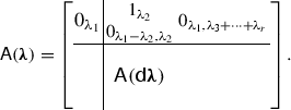
be its companion matrix. Let $A \in \mathrm{M}_n(k)$. It is well-known that there are monic irreducible polynomials $f_1,\cdots ,f_e \in k[X]$ and partitions ${\varvec{\lambda }}_1, \cdots ,\varvec{\lambda }_e$ of positive integers $n_1$,$\cdots$, $n_e$ such that $n = \deg (f_1) n_1 + \cdots + \deg (f_e) n_e$ and A is similar to its (primary) rational canonical form

$$\begin{aligned} \mathrm{diag}\Bigl ( \mathsf {C}\Bigl (f_1^{\lambda _{1,1}}\Bigr ), \cdots , \mathsf {C}\Bigl (f_1^{\lambda _{1,\mathrm {len}({{\varvec{\lambda }}_1})}}\Bigr ), \,\,\cdots \cdots , \,\, \mathsf {C}\Bigl (f_e^{\lambda _{e,1}}\Bigr ), \cdots \, \mathsf {C}\Bigl (f_e^{\lambda _{e_,\mathrm {len}({{\varvec{\lambda }}_e})}}\Bigr ) \Bigr ) \end{aligned}$$

over k. We call $( (f_1,{\varvec{\lambda }}_1), \cdots , (f_e,\varvec{\lambda }_e))$ an elementary divisor vector of A over k; any two elementary divisor vectors of A coincide up to reordering.

1.6 Main results

Recall that k is a number field with ring of integers $\mathfrak {o}$. Throughout, $\mathfrak {p}_v \in \mathrm{Spec}(\mathfrak {o})$ denotes the prime ideal corresponding to a place $v \in \mathcal V_k$ and $q_v = |\mathfrak {o}/\mathfrak {p}_v|$ denotes the residue field size of $k_v$. Our global main result is the following.

Theorem A

Let $S\subset \mathcal V_k$ be finite and $A \in \mathrm{M}_n(\mathfrak {o}_S)$. Let $((f_1,{\varvec{\lambda }}_1), \cdots , (f_e,\varvec{\lambda }_e))$ be an elementary divisor vector of A over k. Write $k_i = k[X]/(f_i)$. Let $\mathfrak {o}_i$ denote the ring of integers of $k_i$. Let $S_i = \{ w \in \mathcal V_{k_i} : \exists v \in S. {w} \mid {v} \}$ and write $\mathfrak {o}_{i,S_i} := (\mathfrak {o}_i)_{S_i}$. Then the following hold:

• (i) There are finitely many places $w_1,\cdots ,w_\ell \in \mathcal V_k{\setminus }S$ and associated rational functions $W_1,\cdots ,W_\ell \in \mathbf {Q}(X)$ such that

  

  (1.1)

  In particular, $\zeta _{A,\mathfrak {o}_S}(s)$ admits meromorphic continuation to the complex plane.

• (ii) The abscissa of convergence $\alpha _{A,\mathfrak {o}_S}$ of $\zeta _{A,\mathfrak {o}_S}(s)$ satisfies $\alpha _{A,\mathfrak {o}_S} = \max \nolimits _{1\leqslant i \leqslant e} \mathrm {len}({{\varvec{\lambda }}_i}) \in \mathbf {N}$.

• (iii) Let $I := \bigl \{ i \in \{ 1,\cdots ,e\} : \mathrm {len}({{\varvec{\lambda }}_i}) = \alpha _{A,\mathfrak {o}_S}\bigr \}$. Then the multiplicity $\beta _{A,\mathfrak {o}_S}$ of the pole of $\zeta _{A,\mathfrak {o}_S}(s)$ at $\alpha _{A,\mathfrak {o}_S}$ satisfies $\beta _{A,\mathfrak {o}_S} = \sum \nolimits _{i\in I} \lambda _{i,-1}$.

As we will see, part (i) is in fact a consequence of a similar formula (5.1) which is valid for almost all local zeta functions $\zeta _{A,\mathfrak {o}_v}(s)$. The exceptional factors $W_u(q_{w_u}^{-s})$ in (1.1) cannot, in general, be omitted, see Example 5.5 below.

We note that the special case $A = 0_n$ in Theorem A is consistent with the well-known formula $\zeta _{\mathfrak {o}_S}(s) \zeta _{\mathfrak {o}_S}(s-1) \cdots \zeta _{\mathfrak {o}_S}(s - (n-1))$ for the zeta function enumerating all finite-index submodules of $\mathfrak {o}_S^n$. We further note that the shape of the right-hand side of (1.1) is rather similar to that of Solomon’s formula [23, Thm 1] for the zeta function enumerating submodules of finite index of a $\mathbf {Z}G$-lattice for a finite group G.

Local functional equations under “inversion of the residue field size” are a common, but not universal, phenomenon in the theory of subobject zeta functions; see [24, 25]. For an extension of number fields $k'/k$ and $v \in \mathcal V_k$, let $\mathrm g_v(k')$ denote the number of places of $k'$ which divide v.

Theorem B

Let $A \in \mathrm{M}_n(k)$ and let $((f_1,{\varvec{\lambda }}_1),\cdots ,(f_e,\varvec{\lambda }_e))$ be an elementary divisor vector of A over k. Write $\varvec{\mu }_i := {\varvec{\lambda }}_i^*$. Then, for almost all $v \in \mathcal V_k$,

(1.2)

We now give a description of the operation “$q_v \rightarrow q_v^{-1}$” in Theorem B. Let $k'/k$ be an extension of number fields, let $\mathfrak {o}'$ be the ring of integers of $k'$, let $v \in \mathcal V_k$, and let $w\in \mathcal V_{k'}$ divide v. It is well-known that $\zeta _{\mathfrak {o}'_w}(s) = 1/(1-q_w^{-s}) = 1/\bigl (1-q_v^{-\mathfrak f(w/v) s}\bigr )$ for some $\mathfrak f(w/v) \geqslant 1$. After excluding finitely many places of k, the local version (5.1) of (1.1) expresses $\zeta _{A,\mathfrak {o}_v}(s)$ as a product of factors of the form $\zeta _{\mathfrak {o}'_w}(as - b)$. The operation “$q_v \rightarrow q_v^{-1}$” is then applied in the evident way to each of these factors.

We note that in the special case that $(A - a 1_n)^n = 0$ for some $a \in k$, the functional equation (1.2) follows from [25, Thm 1.2] (see [25, Rem. 1.5]).

It is natural to ask what properties of A can be inferred from its associated zeta functions. We will make frequent use of the following elementary observation.

Lemma Let $A,B\in \mathrm{M}_n(k)$. Suppose that k[A] and k[B] are similar (i.e. $\mathrm{GL}_n(k)$ -conjugate). Then for almost all $v \in \mathcal V_k$, $\zeta _{A,\mathfrak {o}_v}(s) = \zeta _{B,\mathfrak {o}_v}(s)$.

The following is another consequence of our explicit formulae.

Theorem C

Let $A \in \mathrm{M}_n(k)$ and $B \in \mathrm{M}_m(k)$ be nilpotent. The following are equivalent:

• (i) $n = m$ and A and B are similar.

• (ii) For almost all $v \in \mathcal V_k$, $\zeta _{A,\mathfrak {o}_v}(s) = \zeta _{B,\mathfrak {o}_v}(s)$.

• (iii) There exists a finite $S \subset \mathcal V_k$ such that A and B both have entries in $\mathfrak {o}_S$ and such that $\zeta _{A,\mathfrak {o}_S}(s) = \zeta _{B,\mathfrak {o}_S}(s)$.

The nilpotency condition in Theorem C cannot, in general, be omitted, see Remark 5.8.

The author previously conjectured [17, §8.3] that generic local submodule zeta functions associated with nilpotent matrix algebras have a simple pole at zero. In the present case, our explicit formulae allow us to deduce the following.

Theorem D

Let $A \in \mathrm{M}_n(k)$. Then for almost all $v \in \mathcal V_k$, $\zeta _{A,\mathfrak {o}_v}(s)$ has a pole at zero. Moreover, the following are equivalent:

• (i) For almost all $v \in \mathcal V_k$, $\zeta _{A,\mathfrak {o}_v}(s)$ has a simple pole at zero.

• (ii) There exists $a \in k$ with $(A - a 1_n)^n = 0$.

1.7 Behaviour at zero in general—a conjecture

We use this opportunity to state a generalisation of our conjecture on the behaviour at zero of local submodule zeta functions (see [17, Conj. IV and §8.3]); this generalisation disposes of the mysterious nilpotency assumption found in its precursor.

For a ring R with polynomial submodule growth, a finitely generated R-module M, and $\Omega \subset \mathrm{End}_{R}(M)$, the submodule zeta function $\zeta _{\Omega \curvearrowright M}(s)$ is the Dirichlet series enumerating $\Omega$-invariant R-submodules of finite index of M (cf. [17, Def. 2.1 (ii)]).

Let V be a finite-dimensional vector space over k and let $\mathcal A\subset \mathrm{End}_k(V)$ be an associative, unital subalgebra. Let $\mathrm{rad}(\mathcal A)$ denote the (nil)radical of $\mathcal A$. By the Wedderburn-Malcev Theorem [6, Thm 72.19], there exists a subalgebra $\mathcal S \subset \mathcal A$ such that $\mathcal A = \mathrm{rad}(\mathcal A) \oplus \mathcal S$ as vector spaces (whence $\mathcal S \approx _k \mathcal A/\mathrm{rad}(\mathcal A)$ is semisimple); moreover, $\mathcal S$ is unique up to conjugacy under $(1 + \mathrm{rad}(\mathcal A)) \leqslant \mathcal A^\times$. Choose $\mathfrak {o}$-forms $\mathsf V \subset V$, $\mathsf A \subset \mathrm{End}_{\mathfrak {o}}(\mathsf V)$ and $\mathsf S \subset \mathrm{End}_{\mathfrak {o}}(\mathsf V)$ of V, $\mathcal A$, and $\mathcal S$, respectively. We write $\mathsf X_v := \mathsf X \otimes _{\mathfrak {o}} \mathfrak {o}_v$ in the following.

Conjecture E

For almost all $v \in \mathcal V_k$,

$$\begin{aligned} \frac{\zeta _{\mathsf A_v \curvearrowright \mathsf V_v}(s)}{\zeta _{\mathsf S_v \curvearrowright \mathsf V_v}(s)} \Biggm \vert _{s=0} = 1. \end{aligned}$$

This conjecture reduces to the behaviour predicted in [17, §8.3] in the “nilpotent case” $\mathcal A = \mathrm{rad}(\mathcal A) \oplus k 1_V$. In order to make Conjecture E more explicit, we recall Solomon’s formula for $\zeta _{\mathsf S_v \curvearrowright \mathsf V_v}(s)$. Let $\mathcal S = \mathcal S_1 \oplus \cdots \oplus \mathcal S_r$ be the Wedderburn decomposition of the semisimple algebra $\mathcal S$ (so that each $\mathcal S_i$ is simple). Let $W_i$ be a simple $\mathcal S_i$-module and decompose $V = V_1 \oplus \cdots \oplus V_r$, where $V_i$ is isomorphic to $W_i^{m_i}$ and $\mathcal S$ acts diagonally on V. Let $k_i$ be the centre of $\mathcal S_i$ and let $\mathfrak {o}_i$ be the ring of integers of $k_i$. Finally, let $e_i$ be the Schur index of the central simple $k_i$-algebra $\mathcal S_i$ and define $n_i$ by $\dim _{k_i}(\mathcal A_i)= n_i^2$.

Theorem 1.3

([23, §4]) For almost all $v \in \mathcal V_k$,

$$\begin{aligned} \zeta _{\mathsf S_v \curvearrowright \mathsf V_v}(s) = \prod _{i=1}^r \prod _{j=1}^{m_i e_i} \prod _{\begin{array}{c} w \in \mathcal V_{k_i}\\ {w} \mid {v} \end{array}} \zeta _{\mathfrak {o}_{i,w}}(n_is - j + 1). \end{aligned}$$

(1.3)

The special case $\mathcal A = k[\alpha ]$ ($\alpha \in \mathrm{End}_k(V)$) of Conjecture E follows from Theorem 1.3 and Theorem 5.1 below.

For a more abstract interpretation of Conjecture E, note that we may identify $\mathcal S$ acting on V with $\mathcal A/\mathrm{rad}(\mathcal A)$ acting (faithfully) on the semi-simplification of V as an $\mathcal A$-module (i.e. the direct sum of the composition factors of V as an $\mathcal A$-module).

1.8 Overview

In order to derive Theorems A–D, we proceed as follows. In Sect. 2, we reduce the computation of $\zeta _{A,\mathfrak {o}_S}(s)$ to the case that the minimal polynomial of A over k is a power of an irreducible polynomial. In Sect. 3, we then further reduce to the case that A is nilpotent. The heart of this article, Sect. 4, is then devoted to the explicit determination of $\zeta _{A,\mathfrak {o}_v}(s)$ for nilpotent A and almost all $v \in \mathcal V_k$; as a by-product, in Theorem 4.4, we compute the ideal zeta function of the 2-dimensional ring $\mathbf {Z}[[ X]]$. We then combine our findings and derive Theorems A–D in Sect. 5. Finally, as an application, in Sect. 6, we use Theorem A to compute the abscissae of convergence of some (largely unknown) submodule and ideal zeta functions.

1.9 Notation

Throughout, $\mathbf {N}= \{ 1,2,\cdots \}$ and $\delta _{ij}$ denotes the Kronecker symbol. The symbol “$\subset$” indicates not necessarily proper inclusion. We use $\approx _R$ to denote both the similarity of matrices over R and the existence of an R-isomorphism. Matrices act by right-multiplication on row vectors. Matrix sizes are indicated by single subscripts for square matrices and double subscripts in general; in particular, $1_n$ and $0_{m,n}$ denote the $n\times n$ identity and $m\times n$ zero matrix, respectively.

We say that a property depending on S holds for sufficiently large finite $S \subset \mathcal V_k$, if there exists a finite $S_0 \subset \mathcal V_k$ such that the property holds for all finite $S \subset \mathcal V_k$ with $S \supset S_0$. Given $v \in \mathcal V_k$, we write for the v-adic absolute value on $k_v$ with $|{\pi }|_v = q_v^{-1}$ for $\pi \in \mathfrak {p}_v{\setminus }\mathfrak {p}_v^2$.

By a p-adic field, we mean a finite extension K of the p-adic numbers $\mathbf {Q}_p$ for some prime p. We let $\mathfrak {O}_K$ denote the valuation ring of K and write $q_K$ for the residue field size of K. Furthermore, $\nu _K$ and denote the additive valuation and absolute value on K, respectively, normalised such that any uniformiser $\pi$ satisfies $\nu _K(\pi ) = 1$ and $|{\pi }|_K = q^{-1}_K$. When the reference to K is clear, we occasionally omit the subscript “K”.

2 Reduction to the case of a primary minimal polynomial

By the following, up to enlarging S, we may reduce the computation of $\zeta _{A,\mathfrak {o}_S}(s)$ to the case where the minimal polynomial of A over k is primary (i.e. a power of an irreducible polynomial).

Proposition 2.1

Let $A \in \mathrm{M}_n(k)$. Let $f = f_1 \cdots f_e$ be a factorisation of the minimal polynomial f of A over k into a product of pairwise coprime monic polynomials $f_i \in k[X]$. Let $A_i \in \mathrm{M}_{n_i}(k)$ denote the matrix of A acting on $\mathrm{Ker}(f_i(A))$ with respect to an arbitrary k-basis. Then for almost all $v \in \mathcal V_k$,

$$\begin{aligned} \zeta _{A,\mathfrak {o}_v}(s) = \prod _{i=1}^e \zeta _{A_i,\mathfrak {o}_v}(s). \end{aligned}$$

Proof

It is well-known that $k^n = \mathrm{Ker}(f_1(A)) \oplus \cdots \oplus \mathrm{Ker}(f_e(A))$ is an A-invariant decomposition into subspaces of dimensions $n_1,\cdots ,n_e$, say, and $f_i$ is the minimal polynomial of $A_i$. We may thus assume that $A = \mathrm{diag}(A_1,\cdots ,A_e)$. By the Chinese remainder theorem, for each $i = 1,\cdots ,e$, there exists $g_i \in k[X]$ with $g_i \equiv \delta _{ij} \bmod {f_j}$ for $j = 1,\cdots ,e$. Hence, $g_i(A) = \mathrm{diag}( \delta _{i1} 1_{n_1},\cdots ,\delta _{ie} 1_{n_e}) \in k[A]$. Choose a finite set $S\subset \mathcal V_k$ with $A_i \in \mathrm{M}_{n_i}(\mathfrak {o}_S)$ and $g_i \in \mathfrak {o}_S[X]$ for $i = 1,\cdots ,e$.

Let $v \in \mathcal V_k{\setminus }S$. Write $V := \mathfrak {o}_v^n$. The block diagonal shape of A yields an A-invariant decomposition $V = V_1 \oplus \cdots \oplus V_e$ into free $\mathfrak {o}_v$-modules of ranks $n_1,\cdots ,n_e$. Note that A acts as $A_i$ on each $V_i$ and that each $g_i(A)$ acts as the natural map $V \twoheadrightarrow V_i \hookrightarrow V$. Let $U \leqslant V$ be an $\mathfrak {o}_v$-submodule. If U is A-invariant, then it decomposes as $U = U_1 \oplus \cdots \oplus U_e$ for $A_i$-invariant submodules $U_i \leqslant V_i$. We conclude that $(U_1,\cdots ,U_e) \mapsto U_1 \oplus \cdots \oplus U_e$ defines a bijection from

$$\begin{aligned} \Bigl \{ (U_1,\cdots ,U_e) : U_i \leqslant _{\mathfrak {o}_v} V_i \text { and } U_i A_i \leqslant U_i \text { for } i = 1,\cdots , e \Bigr \} \end{aligned}$$

onto the set of A-invariant submodules of V whence $\zeta _{A,\mathfrak {o}_v}(s) = \zeta _{A_1,\mathfrak {o}_v}(s) \cdots \zeta _{A_e,\mathfrak {o}_v}(s)$. $\square$

3 Reduction to the case of a nilpotent matrix

Recall that $\mathsf {C}(f)$ denotes the companion matrix of a polynomial f. Given a partition ${\varvec{\lambda }} = (\lambda _1,\cdots ,\lambda _r)$, let

$$\begin{aligned} \mathsf {N}({\varvec{\lambda }}) := \mathrm{diag}(\mathsf {C}(X^{\lambda _1}),\cdots ,\mathsf {C}(X^{\lambda _r})). \end{aligned}$$

Suppose that the minimal polynomial of $A \in \mathrm{M}_n(k)$ is a power of an irreducible polynomial f; we then say that A is (f-)primary. The elementary divisors of A are $f^{\lambda _1},\cdots ,f^{\lambda _r}$ for a unique partition ${\varvec{\lambda }} = (\lambda _1,\cdots ,\lambda _r)$ of $n / \deg (f)$. We call ${\varvec{\lambda }}$ the type of A.

For an extension $k'/k$ of number fields and $S\subset \mathcal V_k$, define

$$\begin{aligned} \mathcal D_{k'/k}(S) = \{ w \in \mathcal V_{k'} : \exists v \in S. {w} \mid {v} \}. \end{aligned}$$

Hence, using the notation from Theorem B, $\#\mathcal D_{k'/k}(S) = \sum \nolimits _{v \in S} \mathrm g_v(k')$.

In this section, we prove the following.

Theorem 3.1

Let $f \in k[X]$ be monic and irreducible. Let $A \in \mathrm{M}_n(k)$ be an f-primary matrix of type ${\varvec{\lambda }}$. Let $k' = k[X]/(f)$, and let $\mathfrak {o}'$ be the ring of integers of $k'$. Then for almost all $v \in \mathcal V_k$,

$$\begin{aligned} \zeta _{A,\mathfrak {o}_v}(s) = \prod _{\begin{array}{c} w \in \mathcal V_{k'} \\ {w} \mid {v} \end{array}} \zeta _{\mathsf {N}({\varvec{\lambda }}),\mathfrak {o}'_w}(s). \end{aligned}$$

Hence, for all sufficiently large finite $S \subset \mathcal V_k$, setting $S' = \mathcal D_{k'/k}(S)$.

$$\begin{aligned} \zeta _{A,\mathfrak {o}_S}(s) = \zeta _{\mathsf {N}({\varvec{\lambda }}),\mathfrak {o}'_{S'}}(s). \end{aligned}$$

Remark 3.2

In [22, §3], the study of the variety of subspaces invariant under an endomorphism of a finite-dimensional real or complex vector space is reduced to the case of a nilpotent endomorphism. Shayman proceeds by first reducing to the case of a primary endomorphism ([22, Thm 2]) and our Proposition 2.1 proceeded along the same lines. In his setting, the minimal polynomial of a primary endomorphism is a power of a linear or quadratic irreducible and he considers these cases separately. His reasoning is similar to arguments employed in our proof of Theorem 3.1 below. We may regard the factorisation of $\zeta _{A,\mathfrak {o}_v}(s)$ obtained by combining Proposition 2.1 and Theorem 3.1 as an arithmetic analogue of the factorisation of the space of A-invariant subspaces in [22, Thm 3]. In [22, §4], Shayman then proceeds to study invariant subspaces of nilpotent matrices in Jordan normal form. For our purposes, a slightly different normal form, introduced in Sect. 4.1, will prove advantageous.

Our proof of Theorem 3.1 requires some preparation.

3.1 A generalised Jordan normal form for primary matrices

Let $\otimes$ denote the usual Kronecker product $[a_{ij}]\otimes B = [a_{ij}B]$ of matrices. The following result is a special case of the “separable Jordan normal form” in [14, §6.2]; it can also be obtained by restriction of scalars from the usual Jordan normal form of an f-primary matrix over a minimal splitting field of f over k.

Proposition 3.3

Let $f \in k[X]$ be monic and irreducible of degree d. Let $A \in \mathrm{M}_n(k)$ be f-primary of type ${\varvec{\lambda }}$. Write $m := n/d$. Then $A\approx _k 1_m \otimes \mathsf {C}(f) + \mathsf {N}({\varvec{\lambda }}) \otimes 1_d$.

Lemma 3.4

Let $f \in k[X]$ be monic and irreducible of degree d, ${\varvec{\lambda }} \vdash m > 0$, and $A = 1_m \otimes \mathsf {C}(f) + \mathsf {N}({\varvec{\lambda }}) \otimes 1_d$. Then $1_m \otimes \mathsf {C}(f) = \mathrm{diag}(\mathsf {C}(f),\cdots ,\mathsf {C}(f)) \in k[A]$.

Proof

Write $\gamma := \mathsf {C}(f)$ and $e := \lambda _1$; note that $X^e$ is the minimal polynomial of $\mathsf {N}({\varvec{\lambda }})$ over every field. We may naturally regard A as an $m\times m$ matrix over the field $k':= k[\gamma ]$. Moreover, we may identify $k' = k[1_m \otimes \mathsf {C}(f)]$ as k-algebras. Thus, $k[A, 1_m \otimes \mathsf {C}(f)] = k'[\gamma 1_m + \mathsf {N}({\varvec{\lambda }})] = k'[\mathsf {N}(\varvec{\lambda })]$ whence the k-dimension of $k[A, 1_m \otimes \mathsf {C}(f)]$ is $|k':k| e = de$. As $f^e$ is the minimal polynomial of A over k, the number de is also the k-dimension of k[A] whence the claim follows. $\square$

Regarding the transition from the number field k to the local ring $\mathfrak {o}_v$, we note that the enveloping algebras of companion matrices take the expected forms over UFDs.

Lemma 3.5

Let R be a UFD and let $f \in R[X]$ be monic. Then evaluation at $\mathsf {C}(f)$ induces an isomorphism $R[X]/(f) \approx _R R[\mathsf {C}(f)]$.

Proof

Let K denote the field of fractions of R. The kernel of the natural map $R[X] \rightarrow R[\mathsf {C}(f)]$ is $I := R[X] \cap f K[X]$ and, clearly, $f R[X] \subset I$. Let $h \in I$ so that $h = fg$ for some $g \in K[X]$. By [4, Thm 7.7.2], there exists $a \in K^\times$ with $af,a^{-1}g \in R[X]$. As f is monic (hence primitive), $a \in A$ whence $g = a(a^{-1}g) \in R[X]$ and $h \in fR[X]$. $\square$

3.2 Properties of S-integers and their completions

Lemma 3.6

Let $k'/k$ be an extension of number fields. Let $\mathfrak {o}'$ be the ring of integers of $k'$. Let $S \subset \mathcal V_k$ be finite and $S' = \mathcal D_{k'/k}(S)$. Then $\mathfrak {o}' \otimes _{\mathfrak {o}} \mathfrak {o}_S \approx _{\mathfrak {o}} \mathfrak {o}'_{S'}$.

Proof

The following argument is taken from [5]: if h is the class number of k and $a \in \mathfrak {o}$ generates the principal ideal $\prod _{v\in S} \mathfrak {p}_v^h$, then $\mathfrak {o}_S = \mathfrak {o}[1/a]$. We conclude that $\mathfrak {o}' \otimes _{\mathfrak {o}} \mathfrak {o}_S = \mathfrak {o}'[1/a] = \mathfrak {o}'_{S'}$. $\square$

Lemma 3.7

Let $f \in k[X]$ be monic and irreducible. Let $k' = k[X]/(f)$ with ring of integers $\mathfrak {o}'$. Then the following holds for all sufficiently large finite $S \subset \mathcal V_k$:

• (i) $\mathfrak {o}_S[X]/(f) \approx _{\mathfrak {o}_S} \mathfrak {o}'_{S'}$, where $S'= \mathcal D_{k'/k}(S)$.

• (ii) $\mathfrak {o}_v[X]/(f) \approx _{\mathfrak {o}_v} \prod \nolimits _{\begin{array}{c} w\in \mathcal V_{k'}\\ {w} \mid {v} \end{array}} \mathfrak {o}'_w$ for $v \in \mathcal V_k\setminus S$.

Proof

We freely use the exactness of localisation and completion; see [10, Prop. 2.5, Thm 7.2]. Let $S_0 \subset \mathcal V_k$ be finite with $f \in \mathfrak {o}_{S_0}[X]$. If $S \supset S_0$, then $\mathfrak {o}_{S_0}[X]/(f) \otimes _{\mathfrak {o}_{S_0}} \mathfrak {o}_S \approx _{\mathfrak {o}_S} \mathfrak {o}_S[X]/(f)$. As $\mathfrak {o}_{S_0}[X]/(f)$ and $\mathfrak {o}'$ both become isomorphic to $k'$ after base change to k, for sufficiently large finite $S \supset S_0$, $\mathfrak {o}_S[X]/(f) \approx _{\mathfrak {o}_S} \mathfrak {o}'_{S'}$ by Lemma 3.6. This proves the first part. For the second part, first note that, using (i) and Lemma 3.6,

$$\begin{aligned} \mathfrak {o}_v[X]/(f) \approx _{\mathfrak {o}_v} \mathfrak {o}_S[X]/(f) \otimes _{\mathfrak {o}_S} \mathfrak {o}_v \approx _{\mathfrak {o}_v} \mathfrak {o}'_{S'} \otimes _{\mathfrak {o}_S} \mathfrak {o}_v \approx _{\mathfrak {o}_v} \mathfrak {o}' \otimes _{\mathfrak {o}} \mathfrak {o}_v. \end{aligned}$$

(3.1)

Write $\mathfrak {o}_{(v)} := \mathfrak {o}_v \cap k$ for the v-adic valuation ring of k. It is easy to see that we may naturally identify $\mathfrak {o}' \otimes _{\mathfrak {o}} \mathfrak {o}_{(v)}$ with the integral closure of $\mathfrak {o}_{(v)}$ in $k'$. The key observation here is that if $a \in k'$ is a root of a monic polynomial $f(X) \in \mathfrak {o}_{(v)}[X]$, then there exists $m \in \mathfrak {o}$ with $v(m) = 0$ and $ma \in \mathfrak {o}'$. Indeed, as in the proof of Lemma 3.6, we find $m \in \mathfrak {o}$ such that for all $w \in \mathcal V_k$, $w(m) > 0$ if and only if some coefficient c of f(X) satisfies $w(c) < 0$. By replacing m by a suitable power, we can ensure that all coefficients of mf(X) belong to $\mathfrak {o}$ whence ma is integral over $\mathfrak {o}$ and thus belongs to $\mathfrak {o}'$.

We conclude (see [13, Ch. II, §8, Exerc. 4]) that the canonical isomorphism $k' \otimes _k k_v \approx _{k_v} \prod \nolimits _{ {w} \mid {v} } k'_w$ ([13, Ch. II, Prop. 8.3]) induces an isomorphism $\mathfrak {o}' \otimes _{\mathfrak {o}} \mathfrak {o}_v \approx _{\mathfrak {o}_v} \prod \nolimits _{ {w} \mid {v} } \mathfrak {o}'_w$. Part (ii) thus follows from the latter isomorphism and (3.1). $\square$

3.3 Proof of Theorem 3.1

Recall that $a_m(A,R)$ denotes the number of A-invariant R-submodules of $R^n$ of index m, where $A \in \mathrm{M}_n(R)$.

Proposition 3.8

Let $R_1,\cdots ,R_r$ be rings with polynomial submodule growth.

• (i) $R := R_1 \times \cdots \times R_r$ has polynomial submodule growth.

• (ii) (Cf. [23, Lem. 1].) Let $A \in \mathrm{M}_n(R)$ and let $A_i$ denote the image of A under the map $\mathrm{M}_n(R) \rightarrow \mathrm{M}_n(R_i)$ induced by the projection $R \rightarrow R_i$. Then $a_m(A,R) = a_m(A_1,R_1) \cdots a_m(A_r,R_r)$ for each $m \in \mathbf {N}$. Thus, $\zeta _{A,R}(s) = \zeta _{A_1,R_1}(s) \cdots \zeta _{A_r,R_r}(s)$.

Proof

Decompose $R^n = R_1^n \times \cdots \times R_r^n$ with R acting diagonally on $R^n$. Multiplication by $e_i = (\delta _{1i},\cdots ,\delta _{ni}) \in R$ acts as the natural map $R^n \rightarrow R_i^n \rightarrow R^n$. Given an $R_i$-submodule $U_i \leqslant R_i^n$ for $i = 1,\cdots ,r$, we obtain an R-submodule $U = U_1 \times \cdots \times U_r$ of $R^n$ and it is easy to see that every R-submodule of $R^n$ is of this form in a unique way. Evidently, U has finite index in $R^n$ if and only if each $U_i$ has finite index in $R_i^n$. Part (i) is immediate and (ii) follows since A acts as $A_i$ on $R_i^n$. $\square$

Proof of Theorem 3.1

Assuming that the finite set $S \subset \mathcal V_k$ is sufficiently large, we can make the following assumptions for all $v \in \mathcal V_k{\setminus }S$:

• (NOR) $A = 1_m \otimes \mathsf {C}(f) + \mathsf {N}({\varvec{\lambda }}) \otimes 1_d \in \mathrm{M}_n(\mathfrak {o}_v)$ for $d = \deg (f)$ and ${\varvec{\lambda }} \vdash m$             (Proposition 3.3).

• (DIA) $1_m \otimes \mathsf {C}(f) \in \mathfrak {o}_v[A]$ (Lemma 3.4).

• (INT) $\mathfrak {o}_v[X]/(f) \approx _{\mathfrak {o}_v} \prod \nolimits _{\begin{array}{c} w \in \mathcal V_{k'}\\ {w} \mid {v} \end{array}} \mathfrak {o}'_w$ (Lemma 3.7).

Let $v \in \mathcal V_k{\setminus } S$. First note that as an $\mathfrak {o}_v$-module, $\mathfrak {o}_v[\mathsf {C}(f)]$ is freely generated by $(1_d,\mathsf {C}(f),\cdots ,\mathsf {C}(f)^{d-1})$. It follows easily that $\mathfrak {o}_v^n$ is free of rank m as an $\mathfrak {o}_v[\mathsf {C}(f)]$-module, where $\mathsf {C}(f)$ acts as $1_m \otimes \mathsf {C}(f)$.

Using Lemma 3.5,(INT) allows us to identify $\mathfrak {o}_v[\mathsf {C}(f)] = \mathfrak {o}_v[X]/(f) = \prod _{ {w} \mid {v} } \mathfrak {o}'_w =: R_v$. Thanks to (DIA), we may then regard A as an $m \times m$ matrix over $R_v$. Moreover, the A-invariant $\mathfrak {o}_v$-submodules of $\mathfrak {o}_v^n$ coincide with the A-invariant $R_v$-submodules of $R_v^m$. By (NOR), the latter $R_v$-submodules are precisely those invariant under . Therefore, $\zeta _{A,\mathfrak {o}_v}(s) = \zeta _{\mathsf {N}({\varvec{\lambda }}),R_v}(s)$. Noticing that the (0, 1)-matrix $\mathsf {N}({\varvec{\lambda }})$ is preserved by each projection $R_v \rightarrow \mathfrak {o}'_w$, Proposition 3.8 shows that $\zeta _{\mathsf {N}({\varvec{\lambda }}),R_v}(s) = \prod \nolimits _{ {w} \mid {v} } \zeta _{\mathsf {N}({\varvec{\lambda }}),\mathfrak {o}'_w}(s)$ which concludes the proof. $\square$

4 The case of a nilpotent matrix

Let ${\varvec{\lambda }} \vdash n$. Recall the definitions of ${{\varvec{\lambda }}}^{-1}({j})$ from the introduction and of $\mathsf {N}({\varvec{\lambda }})$ from Sect. 3.

Definition $W_{{\varvec{\lambda }}}(X,Y) = 1 / \prod \nolimits _{j=1}^n \bigl ( 1 - X^{j-1} Y^{{{\varvec{\lambda }}}^{-1}({j})}\bigr ) \in \mathbf {Q}(X,Y)$.

Equivalently, $W_{{\varvec{\lambda }}}(X,Y) = 1 /\prod \nolimits _{i=1}^{\mathrm {len}({{\varvec{\lambda }}})}\prod \nolimits _{j=1}^{\lambda _i} \bigl (1-X^{\mathsf {\sigma }_{i-1}({\varvec{\lambda }})+j-1} Y^i\bigr )$. This section is devoted to proving the following.

Theorem 4.1

Let ${\varvec{\lambda }} \vdash n$ and let K be a p-adic field. Then

$$\begin{aligned} \zeta _{\mathsf {N}({\varvec{\lambda }}^*),\mathfrak {O}_K}(s) = W_{\varvec{\lambda }}(q_K,q_K^{-s}). \end{aligned}$$

Prior to giving a proof of Theorem 4.1, we record a few consequences.

Corollary 4.2

Let $A \in \mathrm{M}_n(k)$ be nilpotent of type ${\varvec{\lambda }}$ (see Sect. 3). Then for all sufficiently large finite sets $S \subset \mathcal V_k$,

If $A \in \mathrm{M}_n(\mathfrak {o})$ and $A \approx _{\mathfrak {o}} \mathsf {N}({\varvec{\lambda }})$, then we may take $S = \varnothing$.

As an application, we can determine the ideal zeta function of $\mathbf {Z}[X]/(X^n)$. Recall that $\zeta (s)$ denotes the Riemann zeta function.

Corollary 4.3

For every prime p,

$$\begin{aligned} \zeta _{\mathbf {Z}_p[X]/(X^n)}(s) = 1 / \prod \limits _{j=1}^n(1-p^{j-1 - js}). \end{aligned}$$

In particular,

$$\begin{aligned} \zeta _{\mathbf {Z}[X]/(X^n)}(s) = \prod \limits _{j=1}^n \zeta (js - j + 1). \end{aligned}$$

Proof

The matrix of multiplication by X acting on $\mathbf {Z}[X]/(X^n)$ with respect to the basis $(1,X,\cdots ,X^{n-1})$, i.e. the companion matrix of $X^n$, is precisely $\mathsf {N}((n))$. $\square$

Remark The subalgebra zeta functions of $\mathbf {Z}_p[X]/(X^n)$ are known only for $n \leqslant 4$ and sufficiently large primes p. Moreover, the author’s computation of these zeta functions for $n = 4$ relied on fairly involved machine calculations; see [18, §9.2]. (The formula for $\zeta _{\mathbf {Z}_p[X]/(X^4)}(s)$ in [18] takes up about a page in total.)

Subobject zeta functions over rings other than $\mathfrak {o}_S$ or $\mathfrak {o}_v$ have received little attention so far. We obtain the following.

Theorem 4.4

• (i) $\mathbf {Z}[[ X]]$ has polynomial submodule growth.

• (ii) $\zeta _{\mathbf {Z}[[ X ]]}(s) = \prod \nolimits _{j=1}^\infty \zeta (js - j + 1)$ for $\mathrm{Re}(s) > 1$.

Proof

It is well-known that the maximal ideals of $\mathbf {Z}[[ X ]]$ are precisely of the form (X, p) for a rational prime p. It follows that X acts nilpotently on every $\mathbf {Z}[[ X]]$-module of finite length. Hence, if $U \leqslant _{\mathbf {Z}[[ X]]} \mathbf {Z}[[ X]]^d$ has finite index, then U contains $X^n \mathbf {Z}[[ X]]^d$ for some $n \geqslant 1$. As $\mathbf {Z}[[ X]]$ is Noetherian, U thus corresponds to a $\mathbf {Z}[X]$-submodule of $\mathbf {Z}[X]^d/X^n\mathbf {Z}[X]^d$. In particular, (i) follows since $\mathbf {Z}[X]$ has polynomial submodule growth by Theorem 1.1. Moreover, Corollary 4.3 implies the identity in (ii) on the level of formal Dirichlet series.

In order to establish (absolute) convergence, let $s > 1$ be real. By well-known facts on infinite products, $\prod _{j=1}^\infty \zeta (js-j+1)$ converges (absolutely) if and only if the same is true of $F(s) := \sum _{j=1}^\infty (\zeta (js-j+1)-1)$. Using the non-negativity of the coefficients of each Dirichlet series $\zeta (js-j+1)$, we obtain

$$\begin{aligned} F(s)&= \sum _{j=1}^\infty \sum _{n=2}^\infty n^{j-1}(n^j)^{-s} = \sum _{n=2}^\infty g_n n^{-s}, \end{aligned}$$

where

We see that for $N \geqslant 2$,

$$\begin{aligned} \sum _{n=2}^N g_n&\leqslant N \sum _{\begin{array}{c} m \geqslant 2, j \geqslant 1\\ m^j \leqslant N \end{array}} \frac{1}{m} \leqslant N \sum _{m=2}^N \frac{2 \log N}{m} = \mathcal O(N (\log N)^2) = \mathcal O(N^{1+\varepsilon }) \end{aligned}$$

for every $\varepsilon > 0$. In particular, F(s) and $\zeta _{\mathbf {Z}[[ X]]}(s)$ both converge for $\mathrm{Re}(s) > 1$. $\square$

Remark 4.5

• (i) Note, in particular, that $\zeta _{\mathbf {Z}[[ X]]}(s)$ has an essential singularity at $s = 1$ and therefore does not admit meromorphic continuation beyond its abscissa of convergence. This illustrates that Theorem 1.2 (ii) does not carry over to general ground rings with polynomial submodule growth.

• (ii) In view of Theorem 1.1, it is natural to investigate the ideal growth of univariate polynomial rings over suitable 1-dimensional ground rings. Segal [20] showed that if R is a Dedekind domain which is not a field and which has only finitely many ideals of a given finite index, then $\zeta _{R[X]}(s) = \prod _{j=1}^\infty \zeta _R(js - j)$ is an identity of formal Dirichlet series. We note that despite the close similarity between Segal’s formula and Theorem 4.4 (ii), our approach is quite different from his.

In order to prove Theorem 4.1, we employ the p-adic integration machinery from [11]. For a ring R, let $\mathrm{Tr}_n(R)$ denote the R-algebra of upper triangular $n\times n$-matrices over R. Recall that an element of a ring is regular if it is not a zero divisor. Write $\mathrm{Tr}_n^\mathrm {reg}(R) = \{ \varvec{x} \in \mathrm{Tr}_n(R) : \det (\varvec{x}) \in R \text { is regular}\}$. For a p-adic field K, let $\mu _K$ denote the Haar measure on $K^n$ with $\mu _K(\mathfrak {O}_K^n) = 1$.

Proposition 4.6

([11, §3]) Let K be a p-adic field and $A \in \mathrm{M}_n(\mathfrak {O}_K)$. Define $V_K(A) := \bigl \{ \varvec{x} \in \mathrm{Tr}^\mathrm {reg}_n(\mathfrak {O}_K) : \mathfrak {O}_K^n \varvec{x} A \subset \mathfrak {O}_K^n \varvec{x} \bigr \}$ to be the set of upper-triangular $n\times n$ matrices over $\mathfrak {O}_K$ whose rows span an A-invariant $\mathfrak {O}_K$-submodule of finite index of $\mathfrak {O}_K^n$. Then

$$\begin{aligned} \zeta _{A,\mathfrak {O}_K}(s) = (1-q_K^{-1})^{-n} \int \limits _{V_K(A)} |{x_{11}}|_K^{s-1} |{x_{22}}|_K^{s-2} \cdots |{x_{nn}}|_K^{s-n} \mathrm{d}\mu _K(\varvec{x}). \end{aligned}$$

(4.1)

Strategy. In order to prove Theorem 4.1, we proceed as follows. First, in Sect. 4.1, we define a matrix $\mathsf {A}({\varvec{\lambda }})$ which is similar (over $\mathbf {Z}$) to $\mathsf {N}({\varvec{\lambda }}^*)$ so that $\zeta _{\mathsf {N}({\varvec{\lambda }}^*),\mathfrak {O}_K}(s) = \zeta _{\mathsf {A}({\varvec{\lambda }}),\mathfrak {O}_K}(s)$. As we will see in Sect. 4.2, the advantage of $\mathsf {A}({\varvec{\lambda }})$ over $\mathsf {N}(\varvec{\lambda }^*)$ is that the sets $V_K(\mathsf {A}({\varvec{\lambda }}))$ in Proposition 4.6 exhibit a natural, recursive structure. Specifically, we will define $\mathsf {d}{{\varvec{\lambda }}} := (\lambda _2,\cdots ,\lambda _{\mathrm {len}({{\varvec{\lambda }}})})$ and find that $V_K(\mathsf {A}({\varvec{\lambda }}))$ can be described in terms of $V_K(\mathsf {A}(\mathsf {d}{{\varvec{\lambda }}}))$ and membership conditions for generic vectors in generic sublattices. In Sect. 4.3, the geometry of such membership conditions is elucidated by means of suitable (birational) changes of coordinates. Finally, in Sect. 4.4, we combine all these ingredients and prove Theorem 4.1.

4.1 A dual normal form for nilpotent matrices

Definition Let ${\varvec{\lambda }} = (\lambda _1,\cdots ,\lambda _r) \vdash n \geqslant 0$. Define $\mathsf {d}{{\varvec{\lambda }}} := (\lambda _2,\cdots ,\lambda _r)$. We recursively define $\mathsf {A}({\varvec{\lambda }}) \in \mathrm{M}_n(\mathbf {Z})$ as follows:

• (i) If $r \leqslant 1$, define $\mathsf {A}({\varvec{\lambda }}) = 0_n$.

• (ii) If $r > 1$, define

  

  (4.2)

In other words,

(4.3)

By the following, the $\mathsf {A}({\varvec{\lambda }})$ parameterise similarity classes of nilpotent matrices.

Proposition 4.7

$\mathsf {A}({\varvec{\lambda }}^*)$ and $\mathsf {N}(\varvec{\lambda })$ are conjugate by permutation matrices.

Proof

Let $T({\varvec{\lambda }})$ be the Young diagram of ${\varvec{\lambda }}$ and let $V(\varvec{\lambda })$ be the $\mathbf {Z}$-module freely generated by the cells of T. We use “English notation” for Young diagrams—that is, $T({\varvec{\lambda }})$ consists of precisely $\mathrm {len}({{\varvec{\lambda }}})$ left-justified rows, indexed as $1,\cdots ,\mathrm {len}({{\varvec{\lambda }}})$ from top to bottom, such that the ith row contains precisely $\lambda _i$ cells. (See below for an example.)

Define $\Theta ({\varvec{\lambda }})$ to be the endomorphism of $V({\varvec{\lambda }})$ (acting on the right) which sends each cell to its right neighbour if it exists and to zero otherwise. We consider two orderings on the cells of $T({\varvec{\lambda }})$ and describe the associated matrices representing $\Theta ({\varvec{\lambda }})$. The horizontal order is defined by traversing the cells of $T({\varvec{\lambda }})$ from left to right within each row, proceeding from top to bottom. For example, by labelling the cells of T((2, 2, 1)) as $1,\cdots ,5$ according to the horizontal order, we obtain

Clearly, $\mathsf {N}({\varvec{\lambda }})$ is the matrix of $\Theta ({\varvec{\lambda }})$ with respect to the horizontal order.

The vertical order is obtained by traversing the cells of $T({\varvec{\lambda }})$ from top to bottom within each column, proceeding from left to right. In the case of T((2, 2, 1)) from above, the vertical order is thus given by

Write $\varvec{\mu }:= {\varvec{\lambda }}^*$, say $\varvec{\mu }= (\mu _1,\cdots ,\mu _\ell )$. We now show by induction on $\ell$ that the matrix of $\Theta ({\varvec{\lambda }})$ with respect to the vertical order is $\mathsf {A}(\varvec{\mu })$—it then follows, in particular, that $\mathsf {A}(\varvec{\mu })$ and $\mathsf {N}({\varvec{\lambda }})$ are conjugate as claimed.

If $\ell \leqslant 1$, then $\Theta ({\varvec{\lambda }}) = 0$ and $\mathsf {A}(\varvec{\mu }) = 0$ so let $\ell > 1$. Let $t_1,\cdots ,t_n$ be the cells of $T({\varvec{\lambda }})$ according to the vertical order. Then $t_i \Theta ({\varvec{\lambda }}) = t_{\mu _1+i}$ for $1\leqslant i \leqslant \mu _2$ and $t_i \Theta ({\varvec{\lambda }}) = 0$ for $\mu _2 < i \leqslant \mu _1$. Let $\tilde{{\varvec{\lambda }}} := (\mathsf {d}{\varvec{\mu }})^*$ and $\tilde{V} :=\mathbf {Z}t_{\mu _1+1} \oplus \cdots \oplus \mathbf {Z}t_n$. We may naturally identify the endomorphism of $\tilde{V}$ induced by $\Theta ({\varvec{\lambda }})$ with $\Theta (\tilde{{\varvec{\lambda }}})$ acting on $V(\tilde{{\varvec{\lambda }}})$; the defining basis of $\tilde{V}$ is then ordered vertically. By induction, the matrix of $\Theta ({\varvec{\lambda }})$ acting on $\tilde{V}$ with respect to the basis $(t_{\mu _1+1},\cdots ,t_n)$ is therefore $\mathsf {A}(\mathsf {d}{\varvec{\mu }})$ whence the claim follows from the recursive description of $\mathsf {A}(\varvec{\mu })$ in (4.2). $\square$

For ${|{\varvec{\lambda }}|} > 0$, let $\mathsf {B}({\varvec{\lambda }}) \in \mathrm{M}_{{|{\varvec{\lambda }}|},{|\mathsf {d}{{\varvec{\lambda }}}|}}(\mathbf {Z})$ denote the matrix obtained by deleting the first $\lambda _1$ columns of $\mathsf {A}({\varvec{\lambda }})$. The following consequence of (4.3) will be useful below.

Lemma 4.8

$\mathsf {B}({\varvec{\lambda }})$ contains precisely $\lambda _1$ zero rows and by deleting these, the ${|\mathsf {d}{{\varvec{\lambda }}}|}\times {|\mathsf {d}{{\varvec{\lambda }}}|}$ identity matrix is obtained.

4.2 Recursion

In this subsection, we give a recursive description of $V_K(\mathsf {A}({\varvec{\lambda }}))$ (see Proposition 4.6).

Lemma 4.9

Let ${\varvec{\lambda }} = (\lambda _1,\cdots ,\lambda _r) \vdash n$ and let X be the generic upper triangular $n\times n$ matrix. Partition X in the form

where subscripts are added to denote block sizes. Then

Proof

This follows easily from (4.2). $\square$

By Lemmas 4.8–4.9, the $\lambda _1\times {|\mathsf {d}{{\varvec{\lambda }}}|}$ submatrix obtained by considering the first $\lambda _1$ rows of $X\mathsf {A}({\varvec{\lambda }})$ and then deleting the first $\lambda _1$ columns is of the form

(4.4)

where the entries marked “$*$” indicate unspecified but distinct variables taken from $\bar{X}$.

Corollary 4.10

Let ${\varvec{\lambda }} \vdash n$ and let K be a p-adic field. For $\varvec{x} \in \mathrm{Tr}_n(K)$, define $\varvec{x}'$ and $\varvec{x}^{{\varvec{\lambda }}}$ by specialising $X'$ and $X^{{\varvec{\lambda }}}$ from Lemma 4.9 and (4.4), respectively, at $\varvec{x}$. Then

$$\begin{aligned} V_K(\mathsf {A}({\varvec{\lambda }})) = \Bigl \{ \varvec{x} \in \mathrm{Tr}^\mathrm {reg}_n(\mathfrak {O}_K) : \text {(i) }&\text {each row of} \ {\varvec{x}}^{{\varvec{\lambda }}} \text {belongs to } \mathfrak {O}_K^{|{\mathsf {d}{{\varvec{\lambda }}}}|} \varvec{x} ' \text {and } \nonumber \\ \text { (ii) }&\varvec{x}' \in V_K(\mathsf {A}(\mathsf {d}{{\varvec{\lambda }}})) \Bigr \}. \end{aligned}$$

(4.5)

Proof

Let $\varvec{x} \in \mathrm{Tr}_n^\mathrm {reg}(\mathfrak {O}_K)$. Clearly, $\varvec{x} \in V_K(\mathsf {A}({\varvec{\lambda }}))$ if and only if every row of $\varvec{x} \mathsf {A}({\varvec{\lambda }})$ is contained in the $\mathfrak {O}_K$-span of the rows of $\varvec{x}$. By Lemma 4.9 and since $\det (\varvec{x}) \not = 0$, the first $\lambda _1$ rows of $\varvec{x} \mathsf {A}({\varvec{\lambda }})$ satisfy this condition if and only if every row of $\varvec{x}^{{\varvec{\lambda }}}$ is contained in the $\mathfrak {O}_K$-span of the rows of $\varvec{x}'$. Similarly, the rows numbered $\lambda _1 + 1,\cdots ,n$ of $\varvec{x} \mathsf {A}({\varvec{\lambda }})$ are contained in the $\mathfrak {O}_K$-span of $\varvec{x}$ if and only if each row of $\varvec{x}' \mathsf {A}(\mathsf {d}{{\varvec{\lambda }}})$ is contained in the $\mathfrak {O}_K$-span of $\varvec{x}'$ or, equivalently, if $\varvec{x}' \in V_K(\mathsf {A}(\mathsf {d}{{\varvec{\lambda }}}))$. $\square$

4.3 Characterising submodule membership

Condition (i) in (4.5) leads us to investigate pairs $(\varvec{x},\varvec{y}) \in R^n \times \mathrm{Tr}_n(R)$ (where R is a ring) such that $\varvec{x}$ is contained in the row span of $\varvec{y}$ over R. In this subsection, we study the set of all such pairs $(\varvec{x},\varvec{y})$ in the case that $R = \mathfrak {O}_K$ for a p-adic field K.

We write $\mathbf {A}^n = \mathrm{Spec}(\mathbf {Z}[X_1,\cdots ,X_n])$ and $\mathrm{Tr}_n = \mathrm{Spec}(\mathbf {Z}[Y_{ij} : 1\leqslant i \leqslant j \leqslant n])$. Let

$$\begin{aligned} E_n(R) := \bigl \{ (\varvec{x}, \varvec{y}) \in R^n \times \mathrm{Tr}_n(R) : \varvec{x}\in R^n \varvec{y}\bigr \}. \end{aligned}$$

(4.6)

We identify $\mathbf {A}^n\times \mathrm{Tr}_n = \mathrm{Spec}(\mathbf {Z}[X_1,\cdots ,X_n, Y_{11},\cdots ,$ $Y_{1n},Y_{22}, \cdots , Y_{nn}])$. Define

$$\begin{aligned} \mathcal {C}_n := \bigl \{ (\alpha ,\omega ) \in \mathbf {R}_{\geqslant 0}^n \times \mathrm{Tr}_n(\mathbf {R}_{\geqslant 0}) : \omega _{ii} \leqslant \alpha _i \text { for } 1 \leqslant i \leqslant n \bigr \}. \end{aligned}$$

(4.7)

For a p-adic field K, we extend $\nu _K$ to families of elements of K via $\nu _K(a_1,\cdots ,a_m) = (\nu _K(a_1),\cdots ,\nu _K(a_m))$ and write

$$\begin{aligned} \mathcal {C}_n(K) := \Bigl \{ (\varvec{x},\varvec{y}) \in K^n \times \mathrm{Tr}_n(K) : (\nu _K(\varvec{x}),\nu _K(\varvec{y})) \in \mathcal {C}_n\Bigr \} \subset \mathfrak {O}_K^n \times \mathrm{Tr}_n^\mathrm {reg}(\mathfrak {O}_K). \end{aligned}$$

The following lemma will play a key role in our proof of Theorem 4.1. It shows that away from sets of measure zero, a suitable $\mathbf {Z}$-defined change of coordinates (defined independently of K) transforms $E_n(\mathfrak {O}_K)$ into $\mathcal {C}_n(K)$.

Lemma 4.11

There exist

• closed subschemes $V_n,V_n' \subset \mathbf {A}^n \times \mathrm{Tr}_n$ of the form $f_n = 0$ and $f_n'= 0$, respectively, where $f_n,f_n' \in \mathbf {Z}[\varvec{X}, \varvec{Y}]$ are non-zero non-units, and

• an isomorphism $\varphi _n :(\mathbf {A}^n\times \mathrm{Tr}_n){\setminus }V_n \rightarrow (\mathbf {A}^n\times \mathrm{Tr}_n){\setminus }V_n'$

such that the following conditions are satisfied:

• (i) For each p-adic field K, $\varphi _n^K( E_n(\mathfrak {O}_K) \setminus V_n(\mathfrak {O}_K)) = \mathcal {C}_n(K){\setminus }V_n'(\mathfrak {O}_K)$, where $\varphi _n^K$ denotes the map induced by $\varphi _n$ on K-points.

• (ii) The Jacobian determinant of $\varphi _n$ is identically 1.

• (iii) $\varphi _n$ commutes with (the appropriate restrictions of) the projection of $\mathbf {A}^n \times \mathrm{Tr}_n$ onto $\mathrm{Tr}_n$ and (the restrictions of) the projection onto the first coordinate of $\mathbf {A}^n$.

Example ($n=2$) Let K be a p-adic field; we drop the subscripts “K” in the following. Let $x,y,a,b,c \in \mathfrak {O}$ and suppose that $x (ay - bx) a b c\not = 0$. Define $y' := y - \frac{x}{a} b \in K$ and note that $y' \not = 0$. Then if and only if $\nu (a) \leqslant \nu (x)$ and $(x,y) - \frac{x}{a} (a,b) = (0,y') \in \mathfrak {O}(0,c)$; the latter condition is equivalent to $\nu (c) \leqslant \nu (y')$ and implies that $y' \in \mathfrak {O}$. We see that the map $((x,y),\bigl [{\begin{matrix} a &{} b\\ 0 &{} c\end{matrix}}\bigr ]) \mapsto ((x,y'),\bigl [{\begin{matrix} a &{} b\\ 0 &{} c\end{matrix}}\bigr ])$ has the properties of $\varphi _2$ stated in Lemma 4.11.

Proof of Lemma 4.11

We proceed by induction. For $n = 1$, we let $f_1 = f_1' = X_1 Y_{11}$ and define $\varphi _1$ to be the identity. Clearly, (i)–(iii) are satisfied.

Let $n > 1$ and suppose that $\varphi _{n-1}$ with the stated properties has been defined. Let K be a p-adic field and let $(\varvec{x},\varvec{y}) \in K^n\times \mathrm{Tr}_n(K)$ with $x_1 y_{11} \not = 0$. We again drop the subscripts “K”. Gaussian elimination shows that $(\varvec{x},\varvec{y}) \in E_n(\mathfrak {O})$ if and only if the following conditions are satisfied:

• (a) $x_i, y_{ij} \in \mathfrak {O}$ for $1\leqslant i \leqslant j \leqslant n$,

• (b) $\frac{x_1}{y_{11}} \in \mathfrak {O}$, and

• (c) .

We will now simplify (c) using a change of coordinates. For $2 \leqslant j \leqslant n$, let $x_j' := x_j - \frac{x_1}{y_{11}} y_{1j}$. Write $x_1' := x_1$ and $\varvec{x}' := (x_1',\cdots ,x_n')$. Note that $(\varvec{x},\varvec{y}) \mapsto (\varvec{x}',\varvec{y})$ is an automorphism of the complement of $Y_{11} = 0$ in $\mathbf {A}^n \times \mathrm{Tr}_n$ and that the Jacobian determinant of this map is identically 1.

Assuming that $y_{ij} \in \mathfrak {O}$ for $1\leqslant i \leqslant j \leqslant n$ and $\frac{x_1}{y_{11}} \in \mathfrak {O}$, we see that $x_j \in \mathfrak {O}$ if and only if $x_j' \in \mathfrak {O}$. Hence, $(\varvec{x},\varvec{y}) \in E_n(\mathfrak {O})$ if and only if (b) and the following two conditions are satisfied:

• (a’) $x_i', y_{ij} \in \mathfrak {O}$ for $1\leqslant i \leqslant j \leqslant n$,

• (c’) .

After excluding suitable hypersurfaces, our inductive hypothesis allows us to perform another change of coordinates, replacing $x_2', \cdots ,x_n'$ by $x_2'', \cdots ,x_n''$, say, such that $(\varvec{x},\varvec{y}) \in E_n(K)$ if and only if the following conditions are satisfied:

• (a”) $x_i'', y_{ij} \in \mathfrak {O}$ for $1\leqslant i \leqslant j \leqslant n$ (where $x_1'' := x_1' = x_1$) and

• (c”) $\nu (y_{ii}) \leqslant \nu (x_i'')$ for $1 \leqslant i \leqslant n$;

note that (b) is implied by the case $i = 1$ of (c”).

For (i), assuming that the product of all $x_i''$ and $y_{ij}$ is non-zero, conditions (a”) and (c”) are both satisfied if and only if $(\varvec{x}'',\varvec{y}) \in \mathcal {C}_n(K)$, where $\varvec{x}'' := (x_1'',\cdots , x_n'')$. The change of coordinates $\varvec{x} \mapsto \varvec{x}''$ is defined over $\mathbf {Z}$, does not depend on K, and, does not modify the $x_1$- or $\varvec{y}$-coordinate, as required for (iii); part (ii) follows since $\varphi _n$ is defined as a composite of maps, the Jacobian determinant of each of which is identically 1. $\square$

Remark 4.12

It follows from Lemma 4.11(ii) that the change of variables afforded by $\varphi _n$ does not affect p-adic measures. Moreover, it is well-known that if $0\not = f \in \mathfrak {O}_K[X_1,\cdots ,X_n]$, then the zero locus of f in $\mathfrak {O}_K^n$ has measure zero. We conclude that $V_n$ and $V_n'$ in Lemma 4.11 are without relevance for the computation of the integral in Proposition 4.6.

4.4 Final steps towards Theorem 4.1

By combining Corollary 4.10 and Lemma 4.11, we may reduce the computation of the integral in Proposition 4.6 for $A = \mathsf {A}({\varvec{\lambda }})$ to a purely combinatorial problem.

Proposition 4.13

Let ${\varvec{\lambda }} = (\lambda _1,\cdots ,\lambda _r) \vdash n$ and let K be a p-adic field. Then

$$\begin{aligned} \zeta _{\mathsf {A}({\varvec{\lambda }}),\mathfrak {O}_K}(s) = (1-q_K^{-1})^{-n} \int _{V_{{\varvec{\lambda }}}(\mathfrak {O}_K)} \prod _{i=1}^n |{x_i}|_K^{s-i} \mathrm{d}\mu _K(\varvec{x}), \end{aligned}$$

(4.8)

where $V_{{\varvec{\lambda }}}(\mathfrak {O}_K)$ consists of those $\varvec{x}\in \mathfrak {O}_K^{n(n+1)/2}$ satisfying the following divisibility conditions, where the $y_{i,j,\ell }$ below denote distinct variables among the $x_{n+1},\cdots ,x_{n(n+1)/2}$:

• For $2 \leqslant i \leqslant r$ and $1 \leqslant j \leqslant \lambda _{i}$,

  $$\begin{aligned} {x_{\mathsf {\sigma }_{i-1}({\varvec{\lambda }}) + j}}\mathrel {\Big |}{x_{\mathsf {\sigma }_{i-2}({\varvec{\lambda }})+j}, y_{i,j,1},\cdots ,y_{i,j,j-1}}. \end{aligned}$$

• For $3 \leqslant i \leqslant r$ and $\mathsf {\sigma }_{i-1}({\varvec{\lambda }}) < j \leqslant n$,

  $$\begin{aligned} {x_j}\mathrel {\Big |}{y_{i,j,n+1},\cdots ,y_{i,j,n+\lambda _{i-2}}}. \end{aligned}$$

Remark Since the $y_{i,j,\ell }$ do not appear in the integrand in the right-hand side of (4.8), it is of no consequence precisely which of the $x_{n+1},\cdots ,x_{n(n+1)/2}$ each $y_{i,j,\ell }$ refers to provided that distinct triples $(i,j,\ell )$ yield different $y_{i,j,\ell }$.

Proof of Proposition 4.13

If $r \leqslant 1$, the claim is trivially true so let $r \geqslant 2$.

As our first step, we combine Corollary 4.10 and Lemma 4.11 in order to transform the membership condition (i) in (4.5). Recall that the non-zero entries of $X^{{\varvec{\lambda }}}$ in (4.4) are distinct variables from $X^I$ or $\bar{X}$; in particular, none of the variables in $X^{{\varvec{\lambda }}}$ occurs in $X'$. We may therefore use Lemma 4.11 to transform the membership condition for any fixed row of $\varvec{x}^{{\varvec{\lambda }}}$ to be contained in $\mathfrak {O}_K^{|{\mathsf {d}{{\varvec{\lambda }}}}|} \varvec{x} '$. Condition (iii) in Lemma 4.11 now ensures that the coordinates corresponding to the variables in $X'$ remain unchanged by each such transformation. By applying Lemma 4.11 to each row of $\varvec{x}^{{\varvec{\lambda }}}$ in turn, we thus obtain the given divisibility conditions for $i = 2$ and $i =3$, respectively; here, $x_1,\cdots ,x_n$ correspond to the diagonal entries $x_{11},\cdots ,x_{nn}$ in Proposition 4.6. Condition (iii) in Lemma 4.11 further ensures that the coordinates corresponding to the diagonal entries of X remain unchanged. Condition (ii) in Lemma 4.11 thus implies that the preceding transformations do not affect the integrand in (4.1).

Having transformed condition (i) in (4.5), subsequent steps then recursively apply the same procedure in order to express the condition $\varvec{x}' \in V_K(\mathsf {A}(\mathsf {d}{{\varvec{\lambda }}}))$ in Corollary 4.10 in terms of the stated divisibility conditions, taking into account the evident shifts of variable indices. Crucially, in doing so, none of the diagonal coordinates will ever be modified, again thanks to condition (iii) in Lemma 4.11. Therefore, the divisibility conditions obtained during earlier steps will never be altered by subsequent ones. The claim thus follows by induction. $\square$

Proof of Theorem 4.1

We once again omit subscripts “K” in the following. Moreover, we will make repeated use of the identity

$$\begin{aligned} \int \limits _{\{ (x,y) \in \mathfrak {O}^2 : {x} \mid {y} \}} |{x}|^r |{y}|^s \mathrm{d}\mu (x,y) = \int \limits _{\mathfrak {O}^2}|{x}|^{r+s+1} |{y}|^s \mathrm{d}\mu (x,y) \end{aligned}$$

(4.9)

which follows by performing a change of variables $y = xy'$ on the left-hand side. We will furthermore use the well-known identity $\int _{\mathfrak {O}}|{x}|^s\mathrm{d}\mu (x) = (1-q^{-1})/(1-q^{-s-1})$.

By repeatedly applying (4.9), we can eliminate all the $y_{i,j,\ell }$ variables and rewrite (4.8) as an integral over $\mathfrak {O}^n$. In order to record the effect of this procedure on the integrand, we use ${\varvec{\lambda }}$ to index $x_1,\cdots ,x_n$ as follows. Let $f(i,j) := \mathsf {\sigma }_{i-1}({\varvec{\lambda }}) + j$ and, for $\varvec{x}= (x_1,\cdots ,x_n)$, write $x_{ij} := x_{f(i,j)}$. Define

$$\begin{aligned} U_{{\varvec{\lambda }}}(\mathfrak {O}) := \Bigl \{ \varvec{x}\in \mathfrak {O}^n : {x_{i,j}} \mid {x_{i-1,j}} \text { for } 2 \leqslant i \leqslant r \text { and } 1 \leqslant j \leqslant \lambda _i \Bigr \}. \end{aligned}$$

Proposition 4.7 and repeated applications of (4.9) to (4.8) show that

$$\begin{aligned} \zeta _{\mathsf {N}({\varvec{\lambda }}^*),\mathfrak {O}}(s) = \zeta _{\mathsf {A}({\varvec{\lambda }}),\mathfrak {O}}(s) = (1-q^{-1})^{-n}\int \limits _{U_{{\varvec{\lambda }}}(\mathfrak {O})} F_{{\varvec{\lambda }}}(\varvec{x})\mathrm{d}\mu (\varvec{x}), \end{aligned}$$

where

$$\begin{aligned} F_{{\varvec{\lambda }}}(\varvec{x})&= \prod _{i=1}^r \prod _{j=1}^{\lambda _i} |{x_{ij}}|^{s - f(i,j)} \times \prod _{i=2}^r \prod _{j=1}^{\lambda _i} |{x_{ij}}|^{j-1} \times \prod _{a=3}^r \prod _{i=a}^r \prod _{j=1}^{\lambda _i} |{x_{ij}}|^{\lambda _{a-2}} \\&= \prod _{j=1}^{\lambda _1} |{x_{1j}}|^{s-j} \times \prod _{i=2}^r \prod _{j=1}^{\lambda _i} |{x_{ij}}|^{s - (\lambda _{i-1}+1)}; \end{aligned}$$

the second equality follows since $s - f(i,j) + j - 1 + \sum _{a=3}^i \lambda _{a-2} = s - (\lambda _{i-1} + 1)$ for $2 \leqslant i \leqslant r$ and $1 \leqslant j \leqslant \lambda _i$. Another sequence of applications of (4.9) can be used to remove the divisibility conditions in $U_{{\varvec{\lambda }}}(\mathfrak {O})$, yielding

$\square$

5 Proofs of Theorems A–D

At the heart of our proofs of Theorems A–D lies the following local version of Theorem A.

Theorem 5.1

Let $S\subset \mathcal V_k$ be finite and $A \in \mathrm{M}_n(\mathfrak {o}_S)$. Let $((f_1,{\varvec{\lambda }}_1), \cdots , (f_e,{\varvec{\lambda }}_e))$ be an elementary divisor vector of A over k. Write $k_i = k[X]/(f_i)$. Let $\mathfrak {o}_i$ denote the ring of integers of $k_i$. Then for almost all $v \in \mathcal V_k$,

(5.1)

Proof

Combine Proposition 2.1, Theorem 3.1, and Theorem 4.1. $\square$

The following is a consequence of Proposition 4.6 and well-known rationality results from p-adic integration.

Proposition 5.2

(Cf. [11, §3]) Let K be a p-adic field and let $A \in \mathrm{M}_n(\mathfrak {O}_K)$. Then $\zeta _{A,\mathfrak {O}_K}(s) \in \mathbf {Q}(q_K^{-s})$. Hence, $\zeta _{A,\mathfrak {O}_K}(s)$ admits meromorphic continuation to all of $\mathbf {C}$.

In order to deduce parts (ii)–(iii) of Theorem A, we will use the following corollary to the detailed analysis of analytic properties of subobject zeta functions in [7].

Lemma 5.3

Let $S' \subset \mathcal V_k$ be finite, $S\subset S'$, and let $A \in \mathrm{M}_n(\mathfrak {o}_S)$. Then $\alpha _{A,\mathfrak {o}_S} = \alpha _{A,\mathfrak {o}_{S'}}$ and $\beta _{A,\mathfrak {o}_S} = \beta _{A,\mathfrak {o}_{S'}}$.

Proof

We first argue that $\alpha _{A,\mathfrak {o}_v} < \alpha _{A,\mathfrak {o}_S}$ for each $v \in \mathcal V_k{\setminus }S$. The zeta function $\zeta _{A,\mathfrak {o}_S}(s+n)$ is an Euler product of cone integrals (cf. Proposition 4.6) in the sense of [7, Def. 4.2]; cf. [7, Cor. 5.6]. Using the notation from [7], by [7, Cor. 3.4] (which is correct despite a minor, fixable mistake in [7, Prop. 3.3], see [1, Rem. 4.6]), it follows that each $\alpha _{A,\mathfrak {o}_v}$ for $v \in \mathcal V_k{\setminus }S$ is a number of the form $n-B_j/A_j$ for $j = 1,\cdots ,q$. Hence, by combining [7, Cor. 4.14, Lem. 4.15], for each $v \in \mathcal V_k{\setminus }S$,

$$\begin{aligned} \alpha _{A,\mathfrak {o}_v} < n + \max _{k=1,\cdots ,q} \frac{1-B_k}{A_k} = \alpha _{A,\mathfrak {o}_S}. \end{aligned}$$

Clearly, $0 < \alpha _{A,\mathfrak {o}_{S'}} \leqslant \alpha _{A,\mathfrak {o}_S}$. Define $F(s) = \prod _{v\in S'{\setminus }S}\zeta _{A,\mathfrak {o}_v}(s)$ so that $\zeta _{A,\mathfrak {o}_S}(s) = F(s)\zeta _{A,\mathfrak {o}_{S'}}(s)$ for all $s \in \mathbf {C}$ with $\mathrm {Re}(s) > \alpha _{A,\mathfrak {o}_S} - \delta$ and some constant $\delta > 0$ (see Theorem 1.2). By the above, every real pole of F(s) is less than $\alpha _{A,\mathfrak {o}_S}$. Since F(s) is a non-zero Dirichlet series with non-negative coefficients, we conclude that $F(\alpha _{A,\mathfrak {o}_S}) > 0$. In particular, since $\zeta _{A,\mathfrak {o}_S}(s)$ has a pole at $\alpha _{A,\mathfrak {o}_S}$, the same is true of $\zeta _{A,\mathfrak {o}_{S'}}(s)$ whence $\alpha _{A,\mathfrak {o}_{S'}} \geqslant \alpha _{A,\mathfrak {o}_S}$. Moreover, $F(\alpha _{A,\mathfrak {o}_S}) > 0$ clearly also implies that $\beta _{A,\mathfrak {o}_S} = \beta _{A,\mathfrak {o}_{S'}}$. $\square$

Remark 5.4

• (i) The corresponding statement for subalgebra and submodule zeta functions (proved in the same way) is certainly well-known to experts in the area. Unfortunately, it does not seem to have been spelled out in the literature. For a similar statement in the context of representation zeta functions, see [2, Thm 1.4].

• (ii) While in [7] only the case $k = \mathbf {Q}$, $S = \varnothing$ is discussed, their arguments carry over to the present setting in the expected way (cf. [1] and [9, §4]).

Proof of Theorem A

Part (i) follows from Theorem 5.1 and Proposition 5.2. Let $\varvec{\mu }\vdash n$. We now determine the largest real pole, $\alpha$ say, and its multiplicity, $\beta$ say, of

Write $r = \mathrm {len}({\varvec{\mu }})$. Since $\zeta _{\mathfrak {o}_S}(s)$ has a unique pole at 1 (with multiplicity 1) and $\zeta _{\mathfrak {o}_S}(s_0) \not = 0$ for real $s_0 > 1$,

$$\begin{aligned} \alpha&= \max _{1\leqslant j \leqslant n} \frac{j}{\varvec{\mu }^{-1}(j)} = \max _{1\leqslant i \leqslant r} \max _{1\leqslant j \leqslant \lambda _i} \frac{\mathsf {\sigma }_{i-1}(\varvec{\mu }) +j}{i} = \max _{1\leqslant i \leqslant r} \frac{\mathsf {\sigma }_{i}(\varvec{\mu })}{i} = \mu _1 = \mathrm {len}({\varvec{\mu }^*}), \end{aligned}$$

where the penultimate equality follows since $i \mu _{i+1} \leqslant \mathsf {\sigma }_i(\varvec{\mu })$ and thus $\frac{\mathsf {\sigma }_i(\varvec{\mu })}{i} \geqslant \frac{\mathsf {\sigma }_{i+1}(\varvec{\mu })}{i+1}$ for $1\leqslant i \leqslant r - 1$. Next, $\beta$ is precisely the number of $i \in \{1,\cdots ,r\}$ with $\mu _1 = \frac{\mathsf {\sigma }_i(\varvec{\mu })}{i}$ or, equivalently, the largest $\ell \geqslant 1$ with $\mu _1 = \cdots = \mu _\ell$. In other words, $\beta = \mu ^*_{-1}$.

Parts (ii)–(iii) of Theorem A now follow from Lemma 5.3 and the observation that $\mathsf {Z}(s) > 0$ for $s > \alpha$. $\square$

Example 5.5

The presence of the exceptional factors $W_u(q_{w_u}^{-s})$ in Theorem A is in general unavoidable. For a simple example, let $a \in \mathfrak {o}$ be non-zero and define $A = \bigl [{\begin{matrix} 0 &{} a \\ 0 &{} 0 \end{matrix}}\bigr ]$. Using Proposition 4.6, a simple computation reveals that for $v \in \mathcal V_k$,

(5.2)

note that $\zeta _{A,\mathfrak {o}_v}(s) = \zeta _{\mathfrak {o}_v}(s) \zeta _{\mathfrak {o}_v}(2s - 1)$ whenever $v(a) = 0$. We further note that the exceptional factor in (5.2) in fact belongs to $\mathbf {Z}[q_v^{-s}]$ and is thus regular at $s = 1$; this is consistent with the general fact that for subobject zeta functions, each local abscissa of convergence is strictly less than the associated global one (see the proof of Lemma 5.3). Finally note the failure of (1.2) for the finitely many $v \in \mathcal V_k$ with $v(a) > 0$.

Remark 5.6

In view of a conjecture of Solomon proved by Bushnell and Reiner [3], it is natural to ask if the $W_u \in \mathbf {Q}(X)$ in Theorem A are in fact always elements of $\mathbf {Z}[X]$.

Proof of Theorem B

The claim follows by combining Theorem 5.1 and the following simple observation. Let $k'/k$ be an extension of number fields, let $\mathfrak {o}'$ be the ring of integers of $k'$, and let $v \in \mathcal V_k$ be unramified in $k'$. If $w \in \mathcal V_{k'}$ divides v, define $\mathfrak f(w/v)$ by $q_w = q_v^{\mathfrak f(w/v)}$. Define

$$\begin{aligned} \mathsf {Z}_v(s) = \prod _{\begin{array}{c} w \in \mathcal V_{k'}\\ {w} \mid {v} \end{array}} \zeta _{\mathfrak {o}'_w}(s) = \prod _{\begin{array}{c} w \in \mathcal V_{k'}\\ {w} \mid {v} \end{array}} \bigl (1-q_v^{-\mathfrak f(w/v)s} \bigr )^{-1}. \end{aligned}$$

Then, recalling the definition of $\mathrm g_v(k')$ from p.5 and using $\sum \nolimits _{ {w} \mid {v} } \mathfrak f(w/v) = |k':k|$,

$\square$

Lemma 5.7

Let $S\subset \mathcal V_k$ be finite. Let $\mathsf {Z}(s)$ and $\mathsf {Z}'(s)$ be two Dirichlet series with finite abscissae of convergence. Suppose that $\mathsf {Z}(s) = \prod _{v \in \mathcal V_k\setminus S}\mathsf {Z}_v(s)$ and $\mathsf {Z}'(s) = \prod _{v \in \mathcal V_k\setminus S}\mathsf {Z}'_v(s)$, where each $\mathsf {Z}_v(s)$ and $\mathsf {Z}'_v(s)$ is a series in $q_v^{-s}$ with non-negative real coefficients. Suppose that $\mathsf {Z}(s) = \mathsf {Z}'(s)$ and that $W(X,Y),W'(X,Y) \in \mathbf {Q}(X,Y)$ satisfy $\mathsf {Z}_v(s) = W(q_v,q_v^{-s})$ and $\mathsf {Z}'_v(s) = W'(q_v,q_v^{-s})$ for almost all $v\in \mathcal V_k \setminus S$. Then $W(X,Y) = W'(X,Y)$.

Proof

Let $S_0$ be the set of rational primes which are divisible by at least one element of S. For a rational prime $p\not \in S_0$, define $\mathsf {Z}_p(s) = \prod _{{v \in \mathcal V_k, {v} \mid {p} }} \mathsf {Z}_v(s)$ and define $\mathsf {Z}'_p(s)$ in the same way. Assuming that $\mathsf {Z}(s) = \mathsf {Z}'(s)$, it is well-known that the coefficients of the Dirichlet series $\mathsf {Z}(s)$ and $\mathsf {Z}'(s)$ coincide. We conclude that $\mathsf {Z}_p(s) = \mathsf {Z}'_{p}(s)$ for $p \not \in S_0$. By Chebotarev’s density theorem, there exists an infinite set of rational primes P such that each $p\in P$ splits completely in k. Writing $d = |k:\mathbf {Q}|$, for almost all $p \in P$, we thus have $W(p,p^{-s})^d = \mathsf {Z}_p(s) = \mathsf {Z}'_p(s) = W'(p,p^{-s})^d$ which easily implies $W(X,Y)^d = W'(X,Y)^d$. Thus, $W(X,Y)/W'(X,Y)$ is a dth root of unity in $\mathbf {R}(X,Y)$ and hence in $\mathbf {R}$, for the latter is algebraically closed in the former (see [4, Prop. 11.3.1]). The non-negativity assumptions on the coefficients of $\mathsf {Z}_v(s)$ and $\mathsf {Z}'_v(s)$ as series in $q_v^{-s}$ now imply $W(X,Y) = W'(X,Y)$. $\square$

Proof of Theorem C

The implications “(i)$\Rightarrow$(ii)$\Rightarrow$(iii)” in Theorem C are obvious. Suppose that (iii) holds. Let ${\varvec{\lambda }}$ and $\varvec{\mu }$ be the types of the matrices A and B, respectively. By Theorem 5.1 and the preceding lemma, $W_{{\varvec{\lambda }}}(X,Y) = W_{\varvec{\mu }}(X,Y)$. It is easy to see that the binomials $1-X^aY^b$ for $a \geqslant 0$ and $b \geqslant 1$ freely generate a free abelian subgroup of $\mathbf {Q}(X,Y)^\times$. Hence, ${\varvec{\lambda }} = \varvec{\mu }$ and A and B are similar. $\square$

Remark 5.8

If A is nilpotent and $\alpha \in k^\times$, then A and $A + \alpha 1_n$ give rise to the same local and global zeta functions without A and $A + \alpha 1_n$ being similar. In general, equality of local and global zeta functions associated with non-nilpotent matrices A and B does not suffice to even conclude that the algebras k[A] and k[B] are similar. We give two examples to illustrate this behaviour, the first being arithmetic and the second of combinatorial origin.

• (i) By [15], there are monic irreducible polynomials $f,g\in \mathbf {Z}[X]$ of the same degree such that the number fields $\mathbf {Q}[X]/(f)$ and $\mathbf {Q}[X]/(g)$ are non-isomorphic but have the same Dedekind zeta functions; moreover, as explained in [15, §1], every rational prime has the same “splitting type” in each of these two number fields. Consequently, $\zeta _{\mathsf {C}(f),\mathbf {Z}_p}(s) = \zeta _{\mathsf {C}(g),\mathbf {Z}_p}(s)$ for almost all primes p

• (ii) Recall the definition of $W_{{\varvec{\lambda }}}$ from Sect. 4. A simple calculation shows that

  

  Let $a,b \in k^\times$ be distinct and choose $A,B \in \mathrm{M}_9(k)$ to have elementary divisor vectors $((X-a,(3,2), (X-b,(2,1,1)))$ and $((X-a,(2,2)),(X-b,(3,1,1)))$, respectively. Then k[A] and k[B] are not similar but $\zeta _{A,\mathfrak {o}_v}(s) = \zeta _{B,\mathfrak {o}_v}(s)$ for almost all $v \in \mathcal V_k$.

Remark 5.9

We further note that even for nilpotent A, the family of associated functional equations (1.2) in Theorem B does not determine A up to similarity; an example is given by two nilpotent $7\times 7$-matrices with types (3, 1, 1, 1, 1) and (2, 2, 2, 1), respectively.

Proof of Theorem D

By Theorem 5.1, $\zeta _{A,\mathfrak {o}_v}(s)$ has a pole at zero for almost all $v \in \mathcal V_k$. Moreover, again for almost all $v \in \mathcal V_k$, this pole is simple if and only if $e = 1$ and almost all places of k remain inert in $k[X]/(f_1)$; the latter condition is equivalent to $f_1$ being linear. $\square$

6 Applications

6.1 Submodules for unipotent groups

Let $S \subset \mathcal V_k$ be finite, let $\mathsf M$ be a finitely generated $\mathfrak {o}_S$-module, and let $\Omega \subset \mathrm{End}_{\mathfrak {o}_S}(\mathsf M)$. We let $\alpha _{\Omega \curvearrowright \mathsf M}$ denote the abscissa of convergence of $\zeta _{\Omega \curvearrowright \mathsf M}(s)$. As a special case (cf. [17, Rem. 2.2 (ii)])), given a possibly non-associative $\mathfrak {o}_S$-algebra $\mathsf A$ whose underlying $\mathfrak {o}_S$-module is finitely generated, we let $\alpha _{\mathsf A}$ denote the abscissa of convergence of its ideal zeta function $\zeta _{\mathsf A}(s)$, as defined in the introduction. We now illustrate how Theorem A can sometimes be used to determine $\alpha _{\Omega \curvearrowright \mathsf M}$ or $\alpha _{\mathsf A}$ without computing the corresponding zeta function. The key observation is that if $\omega \in \Omega$, then $\alpha _{\Omega \curvearrowright \mathsf M} \leqslant \alpha _{\omega ,\mathfrak {o}}$; by Theorem A(ii), the latter number can be easily read off from an elementary divisor vector of $\omega \otimes _{\mathfrak {o}_S} k$.

We let $\mathrm{U}_n$ denote the group scheme of upper unitriangular $n\times n$ matrices. For ${\varvec{\lambda }} = (\lambda _1,\cdots ,\lambda _r) \vdash n$, we regard $\mathrm{U}_{{\varvec{\lambda }}} := \mathrm{U}_{\lambda _1}\times \cdots \times \mathrm{U}_{\lambda _r}$ as a subgroup scheme of $\mathrm{U}_n$ via the natural diagonal embedding. The case $\mathrm {len}({{\varvec{\lambda }}}) = 1$ of the following has consequences for the ideal growth of nilpotent Lie algebras, see [18, §9.4].

Proposition 6.1

Let ${\varvec{\lambda }} \vdash n$. Then $\alpha _{\mathrm{U}_{{\varvec{\lambda }}}(\mathfrak {o}) \curvearrowright \mathfrak {o}^n} = \mathrm {len}({{\varvec{\lambda }}})$.

Proof

Using the characterisation of $\mathrm{U}_m(k)$ as the centraliser of a maximal flag of subspaces of $k^m$, we see that $\mathfrak {o}^n$ contains a $\mathrm{U}_{{\varvec{\lambda }}}(\mathfrak {o})$-invariant submodule N such that $\mathrm{U}_{{\varvec{\lambda }}}(\mathfrak {o})$ acts trivially on $\mathfrak {o}^n/N$ and $\mathfrak {o}^n/N \approx _{\mathfrak {o}} \mathfrak {o}^{\mathrm {len}({{\varvec{\lambda }}})}$. We conclude that $\alpha _{\mathrm{U}_{{\varvec{\lambda }}}(\mathfrak {o}) \curvearrowright \mathfrak {o}^n} \geqslant \mathrm {len}({{\varvec{\lambda }}})$. For an upper bound, note that $(1 + \mathsf {N}({\varvec{\lambda }})) \in \mathrm{U}_{{\varvec{\lambda }}}(\mathfrak {o})$ whence $\alpha _{\mathrm{U}_{{\varvec{\lambda }}}(\mathfrak {o}) \curvearrowright \mathfrak {o}^n} \leqslant \alpha _{\mathsf {N}({\varvec{\lambda }}),\mathfrak {o}} = \mathrm {len}({{\varvec{\lambda }}})$. $\square$

For $|{{\varvec{\lambda }}}|\leqslant 5$ and almost all $v \in \mathcal V_k$, explicit formulae for $\zeta _{\mathrm{U}_{{\varvec{\lambda }}}(\mathfrak {o}_v)\curvearrowright \mathfrak {o}_v^n}(s)$ have been obtained by the author (see [18, §9.4] and the database included with [19]); the only unknown case for $\mathrm {len}({{\varvec{\lambda }}}) = 6$, namely ${\varvec{\lambda }} = (6)$, seems out of reach at present. In addition to their global abscissae of convergence, the $\zeta _{\mathrm{U}_{{\varvec{\lambda }}}(\mathfrak {o}_v)\curvearrowright \mathfrak {o}_v^n}(s)$ are known to generically satisfy local functional equations under inversion of $q_v$ by [25, §5.2].

6.2 Lie algebras of maximal class

Let $\varvec{\mathfrak g}$ be a finite-dimensional Lie k-algebra. For finite $S\subset \mathcal V_k$, by an $\mathfrak {o}_S$ -form of $\varvec{\mathfrak g}$, we mean a Lie $\mathfrak {o}_S$-algebra $\mathfrak g$ whose underlying module is free and such that $\mathfrak g\otimes _{\mathfrak {o}_S} k \approx _k \varvec{\mathfrak g}$.

Let $\varvec{\mathfrak g}= \varvec{\mathfrak g}^1 \supset \varvec{\mathfrak g}^2\supset \cdots$ be the lower central series of $\varvec{\mathfrak g}$. Recall that $\varvec{\mathfrak g}$ has maximal class if $\varvec{\mathfrak g}$ is nilpotent of class $\dim _k(\varvec{\mathfrak g})-1$. Equivalently, $\varvec{\mathfrak g}$ has maximal class if and only if $\dim _k(\varvec{\mathfrak g}^1/\varvec{\mathfrak g}^{2}) = 2$ and $\dim _k(\varvec{\mathfrak g}^i/\varvec{\mathfrak g}^{i+1}) = 1$ for $1 \leqslant i \leqslant \dim _k(\varvec{\mathfrak g}) - 1$.

Proposition 6.2

Let $\mathfrak g$ be an $\mathfrak {o}_S$-form of a non-abelian finite-dimensional Lie k-algebra of maximal class. Then $\alpha _{\mathfrak g} = 2$.

A proof of Proposition 6.2 using Theorem A will be given below.

We note that Proposition 6.2 is consistent with explicit calculations carried out for specific $\mathbf {Z}$-forms of the Lie algebras $M_3$,$M_4$,$M_5$, and $\mathrm {Fil}_4$ of maximal class and dimension at most 5 over the rationals; see [8, Ch. 2].

Lemma 6.3

Let $S\subset \mathcal V_k$ be finite. Let $\mathfrak g$ be an $\mathfrak {o}_S$-form of a nilpotent Lie k-algebra of finite dimension n. Let $\mathsf A$ be the enveloping unital associative algebra of $\mathrm {ad}(\mathfrak g)$ within $\mathrm{End}_{\mathfrak {o}_S}(\mathfrak g)$.

• (i) For each $\varphi \in \mathsf A$, there exists $c \in \mathfrak {o}_S$ with $(\varphi - c 1_{\mathfrak g})^n = 0$; thus, $\varphi \otimes _{\mathfrak {o}_S} k$ is primary.

• (ii) Let $\varphi \in \mathsf A$ have type ${\varvec{\lambda }}$ over k. Then $\alpha _{\mathfrak g} \leqslant \mathrm {len}({{\varvec{\lambda }}})$.

Proof

The first part follows from Engel’s theorem and the second part is then an immediate consequence of Theorem A(ii). $\square$

Lemma 6.4

Let $\varvec{\mathfrak g}$ be an $(n+2)$-dimensional non-abelian Lie k-algebra of maximal class. Then there exists a k-basis $(x_1,x_2,y_1,\cdots ,y_n)$ of $\varvec{\mathfrak g}$ such that $[x_1,x_2] = y_1$, $[x_1,y_i] = y_{i+1}$ for $1 \leqslant i \leqslant n-1$, and $[x_1,y_n] = 0$.

Proof

Consider the graded Lie algebra $\bigoplus _{i\geqslant 1} \varvec{\mathfrak g}^i/\varvec{\mathfrak g}^{i+1}$ associated with $\varvec{\mathfrak g}$. We claim that there exists an element $a \in \varvec{\mathfrak g}/\varvec{\mathfrak g}^2$ such that maps $\varvec{\mathfrak g}^i/\varvec{\mathfrak g}^{i+1}$ onto $\varvec{\mathfrak g}^{i+1}/\varvec{\mathfrak g}^{i+2}$ for each $i \geqslant 1$. To see that, first note that $[\varvec{\mathfrak g}/\varvec{\mathfrak g}^2,\varvec{\mathfrak g}^i/\varvec{\mathfrak g}^{i+1}] = \varvec{\mathfrak g}^{i+1}/\varvec{\mathfrak g}^{i+2}$ for each $i \geqslant 1$. Let (u, v) be a k-basis of $\varvec{\mathfrak g}/\varvec{\mathfrak g}^2$. Then [u, v] spans $\varvec{\mathfrak g}^2/\varvec{\mathfrak g}^3$. Moreover, if $w_i$ spans $\varvec{\mathfrak g}^i/\varvec{\mathfrak g}^{i+1}$, then the image of at least one of $[u,w_i]$ and $[v,w_i]$ spans $\varvec{\mathfrak g}^{i+1}/\varvec{\mathfrak g}^{i+2}$. Consequently, we may take $a = u + cv$ for almost all $c \in k$.

Given a as above, choose $b \in \varvec{\mathfrak g}/\varvec{\mathfrak g}^2$ such that (a, b) is a basis of $\varvec{\mathfrak g}/\varvec{\mathfrak g}^2$. Let $x_1, x_2 \in \varvec{\mathfrak g}$ be preimages of a and b, respectively. Then, if we define $y_1 = [x_1,x_2]$ and $y_{i+1} = [x_1,y_i]$, we obtain a basis $(x_1,x_2,y_1,\cdots ,y_n)$ of the desired form. $\square$

Proof of Proposition 6.2

By Lemma 5.3 and Remark 5.4(i), we are free to enlarge S as needed. In particular, we may assume that $\mathfrak g/\mathfrak g^2 \approx _{\mathfrak {o}_S} \mathfrak {o}_S^2$ whence $\alpha _{\mathfrak g} \geqslant 2$ follows. Moreover, we may assume that $\mathfrak g$ possesses an $\mathfrak {o}_S$-basis $(x_1,x_2,y_1,\ldots ,y_n)$ as in by Lemma 6.4. The matrix of with respect to the basis $(x_2,y_1,\ldots ,y_n,x_1)$ is precisely $\mathsf {N}((n+1,1))$ whence $\alpha _{\mathfrak g} \leqslant 2$ follows from Theorem A. $\square$

References

Avni, N., Klopsch, B., Onn, U., Voll, C.: Representation zeta functions of compact \(p\)-adic analytic groups and arithmetic groups. Duke Math. J. 162(1), 111–197 (2013). doi:10.1215/00127094-1959198
Avni, N., Klopsch, B., Onn, U., Voll, C.: Arithmetic groups, base change, and representation growth. Geom. Funct. Anal. 26(1), 67–135 (2016). doi:10.1007/s00039-016-0359-6
Bushnell, C.-J., Reiner, I.: Zeta functions of arithmetic orders and Solomon’s conjectures. Math. Z. 173(2), 135–161 (1980). doi:10.1007/BF01159955
Cohn, P.M.: Basic algebra, Springer-Verlag London, Ltd., London (2003) doi:10.1007/978-0-85729-428-9, Groups, rings and fields
Conrad, B.: The lattice of \(S\)-integers. http://math.stanford.edu/~conrad/248APage/handouts
Curtis, C.W., Reiner, I.: Representation theory of finite groups and associative algebras, Pure and Applied Mathematics, Vol. Interscience Publishers, a division of John Wiley & Sons, New York-London, XI (1962)
du Sautoy, M.P.F., Grunewald, F.J.: Analytic properties of zeta functions and subgroup growth, 2000. Ann. of Math. (2) 152(3), 793–833 (2000). doi:10.2307/2661355
du Sautoy, M.P.F., Woodward, L.: Zeta functions of groups and rings, Lecture Notes in Mathematics, Springer-Verlag, Berlin, 1925 (2008). doi:10.1007/978-3-540-74776-5
Dung, D.H., Voll, C.: Uniform analytic properties of representation zeta functions of finitely generated nilpotent groups (2015) To appear in Trans. Amer. Math. Soc. arXiv:1503.06947
Eisenbud, D.: Commutative algebra, Graduate Texts in Mathematics, Springer-Verlag, New York 150 (1995). doi:10.1007/978-1-4612-5350-1
Grunewald, F.J., Segal, D., Smith, G.C.: Subgroups of finite index in nilpotent groups. Invent. Math. 93(1), 185–223 (1988)
Macdonald, I.G.: Symmetric functions and Hall polynomials, The Clarendon Press, Oxford University Press, New York, Oxford Mathematical Monographs (1979)
Neukirch, J.: Algebraic number theory, Grundlehren der Mathematischen Wissenschaften, Springer-Verlag, Berlin, 322 (1999). doi:10.1007/978-3-662-03983-0
Norman, C.: Finitely generated abelian groups and similarity of matrices over a field, Springer Undergraduate Mathematics Series, Springer-Verlag, London (2012). doi:10.1007/978-1-4471-2730-7
Perlis, R.: On the equation \(\zeta _{K}(s)=\zeta _{K^{\prime }}(s)\). J. Number Theory 9(3):342–360
Ringel, C.M., Schmidmeier, M.: Invariant subspaces of nilpotent linear operators. I, 2008, J. Reine Angew. Math. 614:1–52. doi:10.1515/CRELLE.2008.001
Rossmann, T.: Computing topological zeta functions of groups, algebras, and modules, I. Proc. Lond. Math. Soc. (3) 110(5), 1099–1134 (2015). doi:10.1112/plms/pdv012
Rossmann, T.: Computing local zeta functions of groups, algebras, and modules (preprint) (2016). arXiv:1602.00919
Rossmann, T.: Zeta, version 0.3.1, 2016. See http://www.math.uni-bielefeld.de/~rossmann/Zeta/
Segal, D.: Ideals of finite index in a polynomial ring. Quart. J. Math. Oxford Ser. (2), 48(189):83–92 (1997). doi:10.1093/qmath/48.1.83
Segal, D.: On the growth of ideals and submodules, J. London Math. Soc. (2), 56(2):245–263 (1997). doi:10.1112/S0024610797005425
Shayman, M.A.: On the variety of invariant subspaces of a finite-dimensional linear operator, Trans. Amer. Math. Soc., 274(2):721–747 (1982). doi:10.2307/1999130
Solomon, L.: Zeta functions and integral representation theory. Advances in Math. 26(3):306–326 (1977)
Voll, C.: Functional equations for zeta functions of groups and rings. Ann. of Math. (2) 172(2), 1181–1218 (2010). doi:10.4007/annals.2010.172.1185
Voll, C.: Local functional equations for submodule zeta functions associated to nilpotent algebras of endomorphisms (preprint) (2016). arXiv:1602.07025
Voll, C.: Zeta functions of groups and rings—recent developments, Groups St Andrews 2013, London Math. Soc. Lecture Note Ser., 422, Cambridge Univ. Press, Cambridge, 469–492 (2016)
Acknowledgements
I would like to thank Christopher Voll for interesting discussions.
Author information
Authors and Affiliations
Corresponding author
Additional information
Communicated by Andreas Thom.
This work is supported by the DFG Priority Programme “Algorithmic and Experimental Methods in Algebra, Geometry and Number Theory” (SPP 1489).
Rights and permissions
About this article
Cite this article
Rossmann, T. Enumerating submodules invariant under an endomorphism. Math. Ann. 368, 391–417 (2017). https://doi.org/10.1007/s00208-016-1499-6
Received:
Revised:
Published:
Issue Date:
DOI: https://doi.org/10.1007/s00208-016-1499-6