Quasiconvexity and Relaxation in Optimal Transportation of Closed Differential Forms

Abstract

This manuscript extends the relaxation theory from nonlinear elasticity to electromagnetism and to actions defined on paths of differential forms. The introduction of a gauge allows for a reformulation of the notion of quasiconvexity in Bandyopadhyay et al. (J Eur Math Soc 17:1009–1039, 2015), from the static to the dynamic case. These gauges drastically simplify our analysis. Any non-negative coercive Borel cost function admits a quasiconvex envelope for which a representation formula is provided. The action induced by the envelope not only has the same infimum as the original action, but has the virtue to admit minimizers. This completes our relaxation theory program.

1 Introduction

The notion of quasiconvexity, the very essence of the theory of direct methods of the calculus of variations developed by Morrey [21], has played an important role in nonlinear elasticity theory [2] and is central in pde’s [14] and the calculus of variations [10], [21]. It is the right notion to guarantee the existence of minimizers for actions on Sobolev spaces. The main goal of this manuscript is to show that a class of actions appearing in the study of dynamical differential forms, can be recast into a class of functionals to which Morrey direct methods of the calculus of variations [21] is applicable. The introduction of gauge differential forms allows one to convert pairs of dynamical differential forms on ${\mathbb {R}}^{n}$ into static exact forms on ${\mathbb {R}}^{n+1}.$ While the former paths of form are subjected to tangential conditions on a $n-$dimensional space, the latter static form is shown to be subjected to a Dirichlet type boundary condition on the $\left( n+1\right) -$dimensional space. As a consequence, relying on prior studies, we initiate and drastically simplify the extension of a relaxation theory to our context.

Let $k\in \left\{ 1,\ldots ,n\right\}$ and let $\Lambda ^{k}\left( {\mathbb {R}}^{n}\right)$ denote the set of $k-$covectors of ${\mathbb {R}}^{n}.$ This manuscript studies actions defined on paths of differential forms on an open bounded smooth contractible set $\Omega \subset {\mathbb {R}}^{n}.$ Any smooth flow map $\Phi :C^{\infty }\big (\left[ 0,1\right] \times \overline{\Omega };\overline{\Omega }\big )$ such that $\Phi \left( t,\cdot \right)$ is a diffeomorphism of $\overline{\Omega }$ onto $\overline{\Omega }$ and any exact $k-$form $f_{0}\in C^{\infty }\left( \overline{\Omega };\Lambda ^{k}\left( {\mathbb {R}}^{n}\right) \right)$ yields a path

$$\begin{aligned} t\mapsto f\left( t,\cdot \right) =\Phi \left( t,\cdot \right) _{\#}f_{0} \end{aligned}$$

(1.1)

of exact $k-$forms on $\overline{\Omega }.$ The path is driven by the velocity ${\mathbf {v,}}$ which, in “Eulerian coordinates”, is uniquely determined by the identity

$$\begin{aligned} \partial _{t}\Phi \left( t,\cdot \right) ={{\mathbf {v}}}\left( t,\cdot \right) \circ \Phi \left( t,\cdot \right) . \end{aligned}$$

In “Eulerian coordinates”, the transport equation in (1.1) reads as

$$\begin{aligned} \partial _{t}f+{\mathcal {L}}_{{{\mathbf {v}}}}f=0, \end{aligned}$$

(1.2)

where ${\mathcal {L}}$ is the Lie derivative acting on the set of vector fields. Let $d_{x}$ denote the exterior derivative on the set of differential forms on $\Omega$ and $\delta _{x}$ denote the adjoint (or co-differential) of $d_{x}.$ Since $f\left( t,\cdot \right)$ is a closed form, we use Cartan formula to infer the existence of a path $t\mapsto g\left( t,\cdot \right)$ of $\left( k-1\right) -$forms such that

$$\begin{aligned} {\mathcal {L}}_{{{\mathbf {v}}}}f=d_{x}g. \end{aligned}$$

(1.3)

When $k=2$ and $n=2m$ is even, for given exact forms $f_{0},f_{1}\in C^{\infty }\left( \overline{\Omega },\Lambda ^{2}\left( {\mathbb {R}}^{2m}\right) \right)$ the prototype action we are interested in is

$$\begin{aligned} {\mathcal {E}}\left( f,{{\mathbf {v}}}\right) =\int _{\left( 0,1\right) \times \Omega }{\frac{1}{2}\,}f^{m}\left| {{\mathbf {v}}}\right| ^{2}\mathrm{d}t. \end{aligned}$$

This represents the total kinetic energy of a physical system over the whole period of time. We may interpret ${{\mathbf {v}}}$ as the velocity of a system of particles whose density is given by the volume form $\varrho =f^{m}.$ By (1.3), the continuity equation holds, namely,

$$\begin{aligned} \partial _{t}\varrho +\nabla _{x}\cdot \left( \varrho \,{{\mathbf {v}}}\right) =0. \end{aligned}$$

The variational problem of interest is then

$$\begin{aligned} \inf _{\left( f,{{\mathbf {v}}}\right) }\left\{ {\mathcal {E}}\left( f,{{\mathbf {v}}}\right) \;:\;\partial _{t}f+{\mathcal {L}}_{{{\mathbf {v}}}}f=0,\quad f(0,\cdot )=f_{0},\ f(1,\cdot )=f_{1}\right\} . \end{aligned}$$

(1.4)

Here $\left( f,{{\mathbf {v}}}\right)$ satisfy some tangential boundary conditions, which will later be specified.

One cannot hope to turn the problem in (1.4) into a convex minimization problem unless $m=1.$ Our strategy is to introduce a gauge which turns (1.4) into a polyconvex minimization problem, so that in the new formulation, the action ${\mathcal {E}}$ is lower semicontinuous (cf. Subsection 3.6).

For general k and n,  we start with a non-negative Borel cost function

$$\begin{aligned} c:\Lambda ^{k}\left( {\mathbb {R}}^{n}\right) \times \Lambda ^{k-1}\left( {\mathbb {R}}^{n}\right) \rightarrow \left[ 0,+\infty \right] , \end{aligned}$$

which is locally bounded on its effective domain. The action induced by the cost c is

$$\begin{aligned} {\mathcal {A}}\left( f,g\right) =\int _{\left( 0,1\right) \times \Omega }c\left( f,g\right) \mathrm{d}t\,\mathrm{d}x. \end{aligned}$$

(1.5)

We sometimes impose a coercivity condition on c: there are $s>1,$$b_{1}>0,$ and $a_{1}\in {\mathbb {R}}$ such that

$$\begin{aligned} c\left( \lambda ,\mu \right) \ge b_{1}\left| \left( \lambda ,\mu \right) \right| ^{s}+a_{1} \end{aligned}$$

(1.6)

for every $\left( \lambda ,\mu \right) \in \Lambda ^{k}\left( {\mathbb {R}} ^{n}\right) \times \Lambda ^{k-1}\left( {\mathbb {R}}^{n}\right) .$ While the purpose of prior studies [11], [12], [13] was to characterize the paths minimizing the action in (1.5) when c is convex, in the current manuscript, we refrain from imposing such a convexity condition. We rather seek the most general conditions, which would ensure that our actions are lower semicontinuous for a topology which allows for a theory for the existence of minimizers. The use of a gauge turns out to be instrumental in linking the right notion of quasiconvexity on c to the classical one, thereby inferring that ${\mathcal {A}}$ is lower semicontinuous (for a topology to be specified).

In order to better convey the approach we develop in the current manuscript, we start by first highlighting the parallel between some of what we do and the well–known use of a gauge in electromagnetism.

Model example step 1: turn${\mathcal {A}}\left( f,g\right)$into$\int C\left( \nabla u\right) \mathrm{d}t\,\mathrm{d}x,$the setting of Morrey [21] .

Suppose for a moment that $\left( k,n\right) =\left( 2,3\right) .$ Let us consider paths of vector fields

$$\begin{aligned} E,B:\left( 0,1\right) \times \Omega \rightarrow {\mathbb {R}}^{3}, \end{aligned}$$

such that E represents an electric field and B represents a magnetic field. The Gauss law for magnetism and the Maxwell–Faraday induction equations are

$$\begin{aligned} \nabla _{x}\cdot B=0\quad \text {and}\quad \partial _{t}B+\nabla _{x}\times E=0. \end{aligned}$$

(1.7)

The ideal Ohm’s law in ideal magnetohydrodynamics links the velocity ${{\mathbf {v}}}$ of the system and the electromagnetic field through the relation

$$\begin{aligned} E=-{{\mathbf {v}}}\times B. \end{aligned}$$

(1.8)

The path of vector fields E is used to obtain a path of $1-$differential form g on $\Omega$ while the path of vector fields B yields a path of $2-$differential form f on $\Omega .$ These differential forms are

$$\begin{aligned} f= & {} B_{1}\mathrm{d}x^{2}\wedge \mathrm{d}x^{3}+B_{2}\mathrm{d}x^{3}\wedge \mathrm{d}x^{1}+B_{3}\mathrm{d}x^{1}\wedge \mathrm{d}x^{2}\quad \text {and}\\ g= & {} E_{1}\mathrm{d}x^{1}+E_{2}\mathrm{d}x^{2}+E_{3}\mathrm{d}x^{3}. \end{aligned}$$

We use the pair of dynamic path $t\mapsto \left( f\left( t,\cdot \right) ,g\left( t,\cdot \right) \right) ,$ defined on $\Omega$ a $3d-$space, to introduce a new static $2-$form h on $\left( 0,1\right) \times \Omega ,$ a higher dimensional set; it is defined as

$$\begin{aligned} h= & {} B_{1}\mathrm{d}x^{2}\wedge \mathrm{d}x^{3}+B_{2}\mathrm{d}x^{3}\wedge \mathrm{d}x^{1}+B_{3}\mathrm{d}x^{1}\wedge \mathrm{d}x^{2}\\&-\,\mathrm{d}t\wedge \left( E_{1}\mathrm{d}x^{1}+E_{2}\mathrm{d}x^{2}+E_{3}\mathrm{d}x^{3}\right) . \end{aligned}$$

The equations in (1.7) are, respectively, equivalent to

$$\begin{aligned} d_{x}f=0\quad \text {and}\quad \partial _{t}f+d_{x}g=0, \end{aligned}$$

(1.9)

while (1.8) means

$$\begin{aligned} g=\left( {{\mathbf {v}}}_{1}\mathrm{d}x^{1}+{{\mathbf {v}}}_{2}\mathrm{d}x^{2}+{{\mathbf {v}}} _{3}\mathrm{d}x^{3}\right) \,\lrcorner \,f, \end{aligned}$$

where $\lrcorner$ denotes the interior product on the set of differential forms. Since $\Omega$ is a contractible set, by the first system of equations in (1.9), $t\mapsto f\left( t,\cdot \right)$ is a path of exact forms. The second system of equations there is equivalent to (1.2 )–(1.3). Let d denote the exterior derivative on the set of forms on $\left( 0,1\right) \times \Omega$ and let $\delta$ denote the adjoint of d. One verifies that (1.9) is equivalent to

$$\begin{aligned} \mathrm{d}h=0. \end{aligned}$$

(1.10)

Hence, there exists a $1-$form on $\left( 0,1\right) \times \Omega ,$ which we denote as

$$\begin{aligned} \omega =-\varphi \,\mathrm{d}t+A_{1}\mathrm{d}x^{1}+A_{2}\mathrm{d}x^{2}+A_{3}\mathrm{d}x^{3}, \end{aligned}$$

such that $\mathrm{d}\omega =h.$ This latter identity reads as

$$\begin{aligned} B=\nabla _{x}\times A\quad \text {and}\quad E=-\nabla _{x}\varphi -\partial _{t}A. \end{aligned}$$

(1.11)

In the physics literature, A is the so-called magnetic vector potential, $\varphi$ is the so-called electric scalar potential and the pair $\left( \varphi ,A\right)$ is referred to as a gauge. The action

$$\begin{aligned} {\mathcal {A}}_{\mathrm {gauge}}\left( B,E\right) =\int _{\left( 0,1\right) \times \Omega }c_{\mathrm {gauge}}\left( B\left( t,x\right) ,E\left( t,x\right) \right) \mathrm{d}t\,\mathrm{d}x \end{aligned}$$

in terms of the gauge $u=(\varphi ,A)$ can be written, for a cost function C,  as

$$\begin{aligned} {\mathcal {A}}_{*}(u)=\int _{\left( 0,1\right) \times \Omega }C\left( \nabla u\right) \mathrm{d}t\,\mathrm{d}x=\int _{\left( 0,1\right) \times \Omega }c_{\mathrm {gauge} }\left( \nabla _{x}\times A,-\nabla _{x}\varphi -\partial _{t}A\right) \mathrm{d}t\,\mathrm{d}x. \end{aligned}$$

The functional ${\mathcal {A}}_{*}$ is in a form where Morrey’s theory [21], linking quasiconvexity to lower semicontinuity, is applicable. However, there is still a missing piece of information due to the fact that in spite of (1.6), there is no choice of $C:{\mathbb {R}}^{4\times 4}\rightarrow \left( -\infty ,+\infty \right]$ and no choice of ${\bar{b}} _{1}>0$ and ${\bar{a}}_{1}\in {\mathbb {R}}$ such that

$$\begin{aligned} C\left( U\right) \ge {\bar{b}}_{1}+{\bar{a}}_{1}\left| U\right| ^{s}. \end{aligned}$$

In conclusion, neither the sublevel sets of $\left\{ {\mathcal {A}}_{*}\le z\right\}$ nor those of $\left\{ {\mathcal {A}}_{\mathrm {gauge}}\le z\right\}$ are expected to be pre-compact for the weak $W^{1,s} -$topology.

Model example step 2: remedies to make $\left\{ \mathbf {{\mathcal {A}} _{\mathrm {gauge}}\le z}\right\}$ pre-compact.

Note that for any real valued function (gauge function) $\psi$ on $\left( 0,1\right) \times \Omega ,$ we have $d\left( \omega +d\psi \right) =\mathrm{d}\omega .$ This shows that $\omega$ is far from being uniquely determined by the identity $\mathrm{d}\omega =h.$ Equivalently, in terms of the electromagnetic fields, the latter identity amounts to asserting that

$$\begin{aligned} B=\nabla _{x}\times \left( A+\nabla _{x}\psi \right) \quad \text {and}\quad E=-\nabla _{x}\left( \varphi -\partial _{t}\psi \right) -\partial _{t}\left( A+\nabla _{x}\psi ,\right) , \end{aligned}$$

and so

$$\begin{aligned} {\mathcal {A}}_{\mathrm {gauge}}\left( A+\nabla _{x}\psi ,\varphi -\partial _{t} \psi \right) ={\mathcal {A}}_{\mathrm {gauge}}\left( A,\varphi \right) . \end{aligned}$$

The action ${\mathcal {A}}_{\mathrm {gauge}}$ then describes physical systems with redundant degrees of freedom, which we turn into our advantage by using the potential $\psi$ as a mere mathematical device which can help gain stronger compactness properties. More precisely, we adjust $\psi$ so that $\delta \left( \omega +\psi \right) =0,$ where we recall that $\delta$ is the adjoint of the operator d. This amounts to assuming, without loss of generality, that we may choose $\left( A,\varphi \right)$ to satisfy

$$\begin{aligned} \partial _{t}\varphi +\nabla \cdot A=0. \end{aligned}$$

(1.12)

The choice of gauge in (1.12) is the so-called Lorenz gauge. A task fulfilled in the current manuscript has been to show that in addition to the requirement (1.12), we may choose $\left( A,\varphi \right)$ with appropriate boundary conditions such that Gaffney inequality holds. Let us first recall the classical Gaffney inequality and then write it in our context. The classical inequality states that there exists a constant $C=C\left( \Omega ,k\right) >0$ such that

$$\begin{aligned} \left\| \nabla \omega \right\| _{L^{2}}^{2}\le C\left( \left\| \mathrm{d}\omega \right\| _{L^{2}}^{2}+\left\| \delta \omega \right\| _{L^{2} }^{2}+\left\| \omega \right\| _{L^{2}}^{2}\right) \end{aligned}$$

for every $\omega \in W_{T}^{1,2}\left( \Omega ;\Lambda ^{k}\right) \cup W_{N}^{1,2}\left( \Omega ;\Lambda ^{k}\right)$ (the T,  respectively the N,  stands for $\nu \wedge \omega =0$ on $\partial \Omega ,$ respectively, $\nu \,\lrcorner \,\omega =0$ on $\partial \Omega$). Here, Gaffney inequality takes the following form: there exists a constant $a>0$ such that under the above appropriate boundary conditions on $\left( A,\varphi \right) ,$ we have

$$\begin{aligned} a\left( \left\| \varphi \right\| _{W^{1,s}}^{s}+\left\| A\right\| _{W^{1,s}}^{s}\right) \le \left\| \partial _{t}\varphi +\nabla _{x}\cdot A\right\| _{L^{s}}^{s}+\left\| \nabla _{x}\times A\right\| _{L^{s} }^{s}+\left\| \nabla _{x}\varphi -\partial _{t}A\right\| _{L^{s}}^{s}\,. \end{aligned}$$

Thus, if we further use (1.12), we have

$$\begin{aligned} a\left( \left\| \varphi \right\| _{W^{1,s}}^{s}+\left\| A\right\| _{W^{1,s}}^{s}\right) \le \left\| \nabla _{x}\times A\right\| _{L^{s} }^{s}+\left\| \nabla _{x}\varphi -\partial _{t}A\right\| _{L^{s}}^{s}\,. \end{aligned}$$

(1.13)

This, together with (1.6), shows that for any $z\in {\mathbb {R}},$ the sublevel set

$$\begin{aligned} \left\{ \left( A,\varphi \right) \;|\;{\mathcal {A}}_{\mathrm {gauge}}\left( A,\varphi \right) \le z\;\text {and}\;\text {(1.12)}\;\text {holds}\right\} \end{aligned}$$

is precompact for the weak $W^{1,s}$ topology.

Back to the general setting.

In the remainder of the introduction, we assume that $f_{0},f_{1}\in L^{s}\left( \Omega ;\Lambda ^{k}\left( {\mathbb {R}}^{n}\right) \right)$ are closed forms, and thus since $\Omega$ is contractible, there exist $F_{0},F_{1}\in W^{1,s}\left( \Omega ;\Lambda ^{k-1}\left( {\mathbb {R}}^{n}\right) \right)$ such that $\mathrm{d}F_{0}=f_{0}$ and $\mathrm{d}F_{1}=f_{1}\,.$ Set

$$\begin{aligned} \widetilde{\omega }\left( t,x\right) =\left( 1-t\right) F_{0}\left( x\right) +t\,F_{1}\left( x\right) . \end{aligned}$$

In order to ease the study of the first part of the manuscript, we first replace $\left( 0,1\right) \times \Omega$ by a bounded open smooth contractible set $O\subset {\mathbb {R}}^{n+1}.$ This can be achieved, for instance, by smoothing out the cylinder $\left( 0,1\right) \times \Omega \subset {\mathbb {R}}^{n+1}$. Then in Subsections 2.4 and 3.5, we return to the study of differential forms on the cylinder $\left( 0,1\right) \times \Omega \subset {\mathbb {R}}^{n+1}$. Given $s \in (1, \infty )$, we study an action on the set ${\mathcal {P}}^{s}\left( \widetilde{\omega }\right)$ which consist of pairs (f, g) such that $f-\mathrm{d}x^{0}\wedge g$ is a closed form on O,

$$\begin{aligned} f\in L^{s}\bigl ( O;\Lambda ^{k}({\mathbb {R}}^{n}) \bigr ) \quad \text {and}\quad g\in L^{s}\bigl ( O;\Lambda ^{k-1}( {\mathbb {R}}^{n}) \bigr ), \end{aligned}$$

and $f-\mathrm{d}x^{0}\wedge g-\mathrm{d}\widetilde{\omega }$ is parallel to the boundary of O (see Definition 2.1). A first goal is to completely characterize the class of cost functions for which ${\mathcal {A}}$ is lower semicontinuous for an appropriate topology on ${\mathcal {P}}^{s}\left( \widetilde{\omega }\right) .$ To achieve this goal, we propose a concept of quasiconvexity in Definition 3.1. We then identify an operator; this is associated with c,  the largest quasiconvex function smaller than c,  which we denote as $Q\left[ c\right] .$ We refer to $Q\left[ c\right]$ as the quasiconvex envelope of c.

Our definition of quasiconvexity is an appropriate variant of the classical one, which Morrey introduced decades ago in the calculus of variations (cf. e.g. [10]); for an intimately related definition we also refer the reader to [3]; for functionals involving several closed differential forms we refer the reader to [23] and [24]. When $k=1$ or $k=n$, quasiconvexity reduces to ordinary convexity, but, in general, and particularly in the case $k=2,$ quasiconvexity is strictly weaker than convexity (see Theorem 3.8). Note that if $k=1$ or $k=n,$ then $Q\left[ c\right] =c^{**}$ the convex envelope of c;  in general (and particularly when $k=2$) $Q\left[ c\right] \ge c^{**},$ but it usually happens that $Q\left[ c\right] \not \equiv c^{**}.$

Under (1.6), Corollary 3.11 establishes existence of minimizers of

$$\begin{aligned} \left( QP\right) \quad \inf \left\{ \int _{O}Q\left[ c\right] \left( f\left( t,x\right) ,g\left( t,x\right) \right) \mathrm{d}t\,\mathrm{d}x\;:\;\left( f,g\right) \in {\mathcal {P}}^{s}\left( \widetilde{\omega }\right) \right\} . \end{aligned}$$

We show that the infimum in $\left( QP\right)$ coincides with the infimum

$$\begin{aligned} \left( P\right) \quad \inf \left\{ \int _{O}c\left( f\left( t,x\right) ,g\left( t,x\right) \right) \mathrm{d}t\,\mathrm{d}x\;:\;\left( f,g\right) \in {\mathcal {P}}^{s}\left( \widetilde{\omega }\right) \right\} \end{aligned}$$

(cf. Theorem 4.5), while no extra conditions are imposed on $c\left( \lambda ,\mu \right)$ beyond the fact that it grows as $\left| \left( \lambda ,\mu \right) \right| ^{s}$ for large values of $\left| \left( \lambda ,\mu \right) \right| ^{s}.$ The infima in $\left( P\right)$ and $\left( QP\right)$ being the same is the basis of our assertion that $\left( QP\right)$ is a relaxation of $\left( P\right) .$

Let us mention that when $k=n,$ so that f is a volume form, and c is convex, problem $\left( P\right)$ falls into the category of the so–called mass transportation problem and has received considerable attention (cf. e.g. [1], [5], [15], [17], [18], [19], [20]). However, while the issues addressed in these works are rather comparable to those addressed in [11], [12], [13], they do not fall into the scope of our current study. Indeed the present approach allows us to extend the above analysis in two directions. First we can deal with quasiconvex and polyconvex functions (cf. Subsection 3.6). We also develop the relaxation setting in order to handle non-quasiconvex integrands.

We close this introduction by drawing the attention of the reader to related works on $A-$quasiconvexity; see [9] and [16].

2 Statement of the Variational Problem

In the present section $O\subset {\mathbb {R}}^{n+1} \simeq {\mathbb {R}} \times {\mathbb {R}}^{n}$ is a bounded open contractible set with smooth boundary and $\nu$ denotes the outward unit normal to $\partial O.$ The variables in O are denoted $\left( t,x\right) \in {\mathbb {R}}\times {\mathbb {R}}^{n}.$ Throughout the manuscript we let $1\le k\le n$ be an integer and $s\in (1,\infty ).$ As is customarily done, $\Lambda ^{l}\left( {\mathbb {R}}^{n}\right)$ is the null set when either l is negative or l is strictly larger than n.

2.1 Notations, Assumptions and Main Variational Problem

Let

$$\begin{aligned} f\in L^{s}\left( O;\Lambda ^{k}\left( {\mathbb {R}}^{n}\right) \right) \quad \text {and}\quad g\in L^{s}\left( O;\Lambda ^{k-1}\left( {\mathbb {R}}^{n}\right) \right) . \end{aligned}$$

(2.1)

We denote as $f^\#=f(t, \cdot )^\#$ the pullback of $f(t, \cdot )$ under the natural projection from ${\mathbb {R}} \times {\mathbb {R}}^{n}$ to ${\mathbb {R}}^{n}$. We similarly define $g^\#$ to obtain on O the differential form of degree k, $h:= f^\# -\mathrm{d}t \wedge g^\#$. In the sequel, by abuse of notation, we write

$$\begin{aligned} f -\mathrm{d}t \wedge g:=f^\# -\mathrm{d}t \wedge g^\#. \end{aligned}$$

Definition 2.1

Let $\widetilde{\omega }\in W^{1,s}\left( O;\Lambda ^{k-1}\left( {\mathbb {R}}^{n+1}\right) \right) .$ We say that $\left( f,g\right) \in {\mathcal {P}}^{s}\left( \widetilde{\omega }\right)$ if (f, g) satisfies (2.1) and, setting $h=f-\mathrm{d}t \wedge g\in L^{s}\left( O;\Lambda ^{k}\left( {\mathbb {R}}^{n+1}\right) \right) ,$

$$\begin{aligned} \mathrm{d}h=0\text { in}\ O\quad \text {and}\quad \nu \wedge h=\nu \wedge d\widetilde{\omega }\text { on }\partial O. \end{aligned}$$

(2.2)

Remark 2.2

• (i) Note that $\mathrm{d}h=d_{x}f+\mathrm{d}t\wedge \left( \partial _{t} f+d_{x}g\right)$, and thus $\mathrm{d}h=0$ means that

  $$\begin{aligned} d_{x}f=0\in \Lambda ^{k+1}\left( {\mathbb {R}}^{n}\right) \quad \text {and}\quad \partial _{t}f+d_{x}g=0\in \Lambda ^{k}\left( {\mathbb {R}}^{n}\right) . \end{aligned}$$

• (ii) The above conditions on h have to be understood in the weak sense, namely

  $$\begin{aligned} \int _{O}\left\langle h;\delta \varphi \right\rangle =\int _{\partial O}\left\langle \nu \wedge \mathrm{d}\widetilde{\omega };\varphi \right\rangle \quad \forall \,\varphi \in C^{1}\left( {\overline{O}};\Lambda ^{k+1}\left( {\mathbb {R}}^{n+1}\right) \right) . \end{aligned}$$

Problem 2.3

(Main problem). Let $c:\Lambda ^{k}\left( {\mathbb {R}}^{n}\right) \times \Lambda ^{k-1}\left( {\mathbb {R}}^{n}\right) \rightarrow \left( -\infty ,\infty \right]$ be Borel measurable and locally bounded on its effective domain. The main problem we consider is

$$\begin{aligned} \left( P\right) \quad \inf \left\{ \int _{O}c\left( f,g\right) :\left( f,g\right) \in {\mathcal {P}}^{s}\left( \widetilde{\omega }\right) \right\} . \end{aligned}$$

We are interested in conditions on the cost function c which ensure that $\left( P\right)$ has a minimizer. More importantly, we are interested in identifying a relaxation problem for $\left( P\right)$ which will be denoted as $\left( QP\right) .$

2.2 Projection of Differential Forms

Decomposition of exterior forms via projection operators.

Let $\left\{ e_{1},\ldots ,e_{n}\right\}$ be the standard orthonormal basis of ${\mathbb {R}}^{n}$ and let $\left\{ {\bar{e}}_{0},{\bar{e}}_{1},\ldots ,{\bar{e}} _{n}\right\}$ be the standard orthonormal basis of ${\mathbb {R}}^{n+1}$ such that the last n entries of ${\bar{e}}_{0}$ are null while the first one equals 1. For $1\le i\le n,$ we denote the dual vector to $e_{i}$ in $\Lambda ^{1}\left( {\mathbb {R}}^{n}\right)$ as $\mathrm{d}x^{i}$ and identify it with the dual vectors to ${\bar{e}}_{i}$ in $\Lambda ^{1}\left( {\mathbb {R}}^{n+1}\right) .$ We write

$$\begin{aligned} x_{0}=t\in {\mathbb {R}}\quad \text {and}\quad \mathrm{d}x^{0}=\mathrm{d}t. \end{aligned}$$

Given $\xi \in \Lambda ^{l}\left( {\mathbb {R}}^{n+1}\right) ,$$0\le l\le n,$

$$\begin{aligned} \xi =\sum _{0\le i_{1}<\cdots <i_{l}\le n}\xi _{i_{1}\cdots i_{l}}\mathrm{d}x^{i_{1} }\wedge \cdots \wedge \mathrm{d}x^{i_{l}}, \end{aligned}$$

we define the projections $\left( \xi ^{x},\xi ^{0}\right) \in \Lambda ^{l}\left( {\mathbb {R}}^{n}\right) \times \Lambda ^{l-1}\left( {\mathbb {R}} ^{n}\right)$ as

$$\begin{aligned} \xi ^{x}&=\pi _{x}\left( \xi \right) =\sum _{1\le i_{1}<\cdots<i_{l}\le n}\xi _{i_{1}\cdots i_{l}}\mathrm{d}x^{i_{1}}\wedge \cdots \wedge \mathrm{d}x^{i_{l}}\\ \xi ^{0}&=\pi _{0}\left( \xi \right) =\sum _{1\le i_{2}<\cdots <i_{l}\le n}\xi _{0i_{2}\cdots i_{l}}\mathrm{d}x^{i_{2}}\wedge \cdots \wedge \mathrm{d}x^{i_{l}} \end{aligned}$$

so that

$$\begin{aligned} \xi =\xi ^{x}+\mathrm{d}x^{0}\wedge \xi ^{0}. \end{aligned}$$

(2.3)

When $l=0,$ we set $\pi _{x}\left( \xi \right) =\xi$ and $\pi _{0}\left( \xi \right) =0.$ When $l\ge 1$, we write

$$\begin{aligned} \xi _{i_{1}\cdots i_{l}}^{x}=\xi _{i_{1}\cdots i_{l}}\quad \text {and}\quad \xi _{i_{2}\cdots i_{l}}^{0}=\xi _{0i_{2}\cdots i_{l}}\,. \end{aligned}$$

The map $\pi _{x}\times \left( -\pi _{0}\right)$ is a bijection of $\Lambda ^{l}\left( {\mathbb {R}}^{n+1}\right)$ onto $\Lambda ^{l}\left( {\mathbb {R}}^{n}\right) \times \Lambda ^{l-1}\left( {\mathbb {R}}^{n}\right)$, and so c can be expressed as a function defined on the former set. We define

$$\begin{aligned} c_{\mathrm {gauge}}:\Lambda ^{l}\left( {\mathbb {R}}^{n+1}\right) \rightarrow \left( -\infty ,+\infty \right] \end{aligned}$$

as

$$\begin{aligned} c_{\mathrm {gauge}}\left( \xi \right) =c\left( \pi _{x}\left( \xi \right) ,-\pi _{0}\left( \xi \right) \right) . \end{aligned}$$

(2.4)

From the above definitions, it is straightforward to obtain the following lemma:

Lemma 2.4

Let $1\le l,m\le n$ be integers, $\xi \in \Lambda ^{l}\left( {\mathbb {R}}^{n+1}\right)$ and $\eta \in \Lambda ^{m}\left( {\mathbb {R}}^{n+1}\right) .$ Then

$$\begin{aligned} \pi _{x}\left( \xi \wedge \eta \right)= & {} \pi _{x}\left( \xi \right) \wedge \pi _{x}\left( \eta \right) \quad \text {and}\\ \pi _{0}\left( \xi \wedge \eta \right)= & {} \left( -1\right) ^{l}\pi _{x}\left( \xi \right) \wedge \pi _{0}\left( \eta \right) +\pi _{0}\left( \xi \right) \wedge \pi _{x}\left( \eta \right) . \end{aligned}$$

Let $r\ge 2$ be an integer, $\xi \in \Lambda ^{l}\left( {\mathbb {R}}^{n+1}\right)$, and let

$$\begin{aligned} \xi ^{r}=\underset{r\text { times}}{\underbrace{\xi \wedge \cdots \wedge \xi }} \end{aligned}$$

(so that $\xi ^{r}=0$ if l is odd or if $r\cdot l>n+1$). Then (inductively),

$$\begin{aligned} \pi _{x}\left( \xi ^{r}\right) =\left[ \pi _{x}\left( \xi \right) \right] ^{r}\quad \text {and}\quad \pi _{0}\left( \xi ^{r}\right) =\left\{ \begin{array}[c]{cl} r\left[ \pi _{x}\left( \xi \right) \right] ^{r-1}\wedge \pi _{0}\left( \xi \right) &{} \text {if }l\text { is even}\\ 0 &{} \text {if }l\text { is odd.} \end{array} \right. \end{aligned}$$

In particular, if l is even and $r\cdot l=n+1,$ then $\pi _{x}\left( \xi ^{r}\right) =0$ (but, in general, $\pi _{0}\left( \xi ^{r}\right) \ne 0$).

Decomposition of differential forms. If $\omega \in W^{1,s}\left( O;\Lambda ^{k}\left( {\mathbb {R}}^{n+1}\right) \right) ,$ then direct computations reveal that

$$\begin{aligned} \mathrm{d}\omega= & {} d_{x}F+\mathrm{d}x^{0}\wedge \left( \partial _{t}F-d_{x}G\right) \in \Lambda ^{k+1}\quad \text {and}\nonumber \\ \delta \omega= & {} \left( \partial _{t}G+\delta _{x}F\right) -\mathrm{d}x^{0}\wedge \delta _{x}G\in \Lambda ^{k-1}, \end{aligned}$$

(2.5)

or, equivalently, in terms of the projections and differential operators,

$$\begin{aligned} \pi _{x} \circ d= & {} d_x \circ \pi _x \quad \text {and}\quad \pi _{0} \circ d = \partial _t \circ \pi _x -d_x \circ \pi _0 \end{aligned}$$

(2.6)

$$\begin{aligned} \pi _{x} \circ \delta= & {} \partial _t \circ \pi _0 +\delta _x \circ \pi _x \quad \text {and}\quad \pi _{0} \circ \delta =-\delta _x \circ \pi _{0}. \end{aligned}$$

(2.7)

2.3 The Gauge Formulation

Intimately related to the previous problem is a new one which uses a kind of gauge.

Problem 2.5

(Gauge formulation). Let O,  $c_{\mathrm {gauge}}$ and $\widetilde{\omega }$ as above. The gauge problem is then defined as

$$\begin{aligned} \left( P_{\mathrm {gauge}}\right) \quad \inf _{\omega }\left\{ \int _{O}c_{\mathrm {gauge}}\left( \mathrm{d}\omega \right) :\omega \in {\mathcal {P}} _{\mathrm {gauge}}^{s}\left( \widetilde{\omega }\right) \right\} , \end{aligned}$$

where

$$\begin{aligned} {\mathcal {P}}_{\mathrm {gauge}}^{s}\left( \widetilde{\omega }\right) =\widetilde{\omega }+W_{0}^{1,s}\left( O;\Lambda ^{k-1}\left( {\mathbb {R}}^{n+1}\right) \right) . \end{aligned}$$

(2.8)

Remark 2.6

In the case $k=1$ (i.e. $\omega$ is a function), we have

$$\begin{aligned} c_{\mathrm {gauge}}\left( \mathrm{d}\omega \right) =c_{\mathrm {gauge}}\left( \nabla \omega \right) =c\left( \pi _{x}\left( \nabla \omega \right) ,-\pi _{0}\left( \nabla \omega \right) \right) =c\left( \nabla _{x}\omega ,-\partial _{t}\omega \right) . \end{aligned}$$

The following proposition shows the equivalence between $\left( P\right)$ and $\left( P_{\mathrm {gauge}}\right)$:

Proposition 2.7

Under the above hypotheses,

$$\begin{aligned} \inf \left( P\right) =\inf \left( P_{\mathrm {gauge}}\right) . \end{aligned}$$

More precisely, if $\omega \in {\mathcal {P}}_{\mathrm {gauge}}^{s}\left( \widetilde{\omega }\right) ,$ then

$$\begin{aligned} \left( f,g\right) =\left( \pi _{x} ,-\pi _{0} \right) (\mathrm{d}\omega ) \in {\mathcal {P}}^{s}\left( \widetilde{\omega }\right) . \end{aligned}$$

Conversely, given $\left( f,g\right) \in {\mathcal {P}}^{s}\left( \widetilde{\omega }\right) ,$ there exists $\omega \in {\mathcal {P}}_{\mathrm {gauge}}^{s}\left( \widetilde{\omega }\right)$ such that

$$\begin{aligned} \left( f,g\right) =\left( \pi _{x} ,-\pi _{0} \right) (\mathrm{d}\omega ). \end{aligned}$$

Proof

Step 1. Let $\omega \in {\mathcal {P}}_{\mathrm {gauge}}^{s}\left( \widetilde{\omega }\right) ,$ write the decomposition $\omega =\pi _{x}\left( \omega \right) +\mathrm{d}x^{0}\wedge \pi _{0}\left( \omega \right) =F+\mathrm{d}x^{0}\wedge G$, and then set

$$\begin{aligned} f=\pi _{x}\left( \mathrm{d}\omega \right) ,\quad g=-\pi _{0}\left( \mathrm{d}\omega \right) \quad \text {and}\quad h=f-\mathrm{d}x^{0}\wedge g. \end{aligned}$$

It follows from (2.6) that

$$\begin{aligned} f=d_{x}F\in L^{s}\left( O;\Lambda ^{k}\left( {\mathbb {R}}^{n}\right) \right) \quad \text {and}\quad g=-\partial _{t}F+d_{x}G\in L^{s}\left( O;\Lambda ^{k-1}\left( {\mathbb {R}}^{n}\right) \right) . \end{aligned}$$

Observe that

$$\begin{aligned} \mathrm{d}h=d_{x}f+\mathrm{d}x^{0}\wedge \left( \partial _{t}f+d_{x}g\right) =0. \end{aligned}$$

Since $\mathrm{d}\omega =h$ in O and $\omega =\widetilde{\omega }$ on $\partial O,$ we have

$$\begin{aligned} \nu \wedge \mathrm{d}\widetilde{\omega }=\nu \wedge h\quad \text {on }\partial O, \end{aligned}$$

and thus $\left( f,g\right) \in {\mathcal {P}}^{s}\left( \widetilde{\omega }\right) .$

Step 2. Conversely, let $\left( f,g\right) \in {\mathcal {P}}^{s}\left( \widetilde{\omega }\right)$ and recall that

$$\begin{aligned} h=f-\mathrm{d}x^{0}\wedge g\in L^{s}\left( O;\Lambda ^{k}\left( {\mathbb {R}} ^{n+1}\right) \right) . \end{aligned}$$

Since

$$\begin{aligned} \mathrm{d}h=0\text { in}\ O\quad \text {and}\quad \nu \wedge h=\nu \wedge d\widetilde{\omega }\text { on }\partial O, \end{aligned}$$

we can find (cf. Theorem 5.3) $\omega \in W^{1,s}\left( O;\Lambda ^{k-1}\left( {\mathbb {R}}^{n+1}\right) \right)$ such that

$$\begin{aligned} \left\{ \begin{array}[c]{cl} \mathrm{d}\omega =h &{} \text {in }O\\ \omega =\widetilde{\omega } &{} \text {on }\partial O. \end{array} \right. \end{aligned}$$

Thus, $\omega \in {\mathcal {P}}_{\mathrm {gauge}}^{s}\left( \widetilde{\omega }\right) .$$\quad \square$

Remark 2.8

Let O and ${\tilde{\omega }}$ be as above. In the proof of Proposition 2.7, the heart of the matter was to know that for any $h\in L^{s}\left( O;\Lambda ^{k}\left( {\mathbb {R}}^{n+1}\right) \right)$ satisfying (2.2), we could find $\omega \in {\tilde{\omega }} \in W^{1,s}\left( O;\Lambda ^{k-1}\left( {\mathbb {R}}^{n+1}\right) \right)$ such that $\mathrm{d}\omega =h.$ We would like to draw the attention of the reader to the fact that if O was only assumed to be a connected bounded open smooth set (not necessarily contractible), an additional condition would have to be imposed on h to obtain the existence of such a $\omega .$ Mainly, we would need to impose the additional requirement that

$$\begin{aligned} \int _{O}\left\langle h;\chi \right\rangle =\int _{\partial O}\left\langle \nu \wedge \widetilde{\omega };\chi \right\rangle \quad \forall \,\chi \in {\mathcal {H}}_{T}\left( O;\Lambda ^{k}\left( {\mathbb {R}}^{n+1}\right) \right) . \end{aligned}$$

Here ${\mathcal {H}}_{T}$ is the set of harmonic forms with vanishing tangential component (see [6], for details).

2.4 The Case of the Cylinder

In Proposition 2.7 (above), the smoothness of the domain $O\subset {\mathbb {R}}^{n+1}$ made it easier to reach our conclusions. We now show how, by reinforcing the hypotheses a little, we can handle the case of the cylinder $O=\left( 0,1\right) \times \Omega \subset {\mathbb {R}}^{n+1}.$ Let $\Omega \subset {\mathbb {R}}^{n}$ be an open bounded smooth convex set. We assume, without loss of generality, that $0\in \Omega$, and so there is a $1-$homogeneous convex function $\varrho _{\Omega }:{\mathbb {R}}^{n}\mapsto [0,\infty )$ smooth except at the origin such that

$$\begin{aligned} \Omega =\left\{ \varrho _{\Omega }<1\right\} \quad \text {and}\quad \partial \Omega =\left\{ \varrho _{\Omega }=1\right\} . \end{aligned}$$

For $\delta \in \left( 0,1/2\right) ,$ we set

$$\begin{aligned} \Omega _{\delta }=\left\{ \varrho _{\Omega }<1-\delta \right\} \quad \text {and}\quad \partial \Omega _{\delta }=\left\{ \varrho _{\Omega } =1-\delta \right\} . \end{aligned}$$

We let $O=\left( 0,1\right) \times \Omega ,$$\nu$ and $\nu _{x}$ denote, respectively, the outward unit normal to $\partial O$ and $\partial \Omega .$ We also let $c:\Lambda ^{k}\left( {\mathbb {R}}^{n}\right) \times \Lambda ^{k-1}\left( {\mathbb {R}}^{n}\right) \rightarrow {\mathbb {R}}$ be Borel measurable and locally bounded. We further assume that there are $a_{1}\,,a_{2}\in {\mathbb {R}}$ and $b_{1},b_{2}>0$ such that

$$\begin{aligned} a_{1}+b_{1}\left| \left( \lambda ,\mu \right) \right| ^{s}\le & {} c\left( \lambda ,\mu \right) \nonumber \\\le & {} a_{2}+b_{2}\left| \left( \lambda ,\mu \right) \right| ^{s},\quad \forall \left( \lambda ,\mu \right) \in \Lambda ^{k}\left( {\mathbb {R}}^{n}\right) \times \Lambda ^{k-1}\left( {\mathbb {R}}^{n}\right) .\quad \nonumber \\ \end{aligned}$$

(2.9)

Definition 2.9

Let $f_{0},f_{1}\in L^{s}\left( \Omega ;\Lambda ^{k}\left( {\mathbb {R}}^{n}\right) \right)$ and $\delta \in \left( 0,1/2\right)$ be such that

$$\begin{aligned} \mathrm {{\text {supp}}}\left( f_{0}\right) \cup \mathrm {{\text {supp}}}\left( f_{1}\right) \subset \Omega _{\delta } \end{aligned}$$

(2.10)

and $d_{x}f_{0}=d_{x}f_{1}=0$ in$\ \Omega .$ This last condition, coupled with (2.10), means that

$$\begin{aligned} \int _{\Omega }\left\langle f_{1};\delta \phi \right\rangle =\int _{\Omega }\left\langle f_{0};\delta \phi \right\rangle =0,\quad \forall \phi \in C^{1}\left( \overline{\Omega };\Lambda ^{k+1}\right) . \end{aligned}$$

Remark 2.10

In view of the above properties of $f_{0}$ and $f_{1}\,,$ we can find ${\overline{F}}_{i}\in W^{1,s}\left( \Omega _{\delta },\Lambda ^{k-1}\left( {\mathbb {R}}^{n}\right) \right) ,$$i=0,1,$ such that

$$\begin{aligned} \left\{ \begin{array}[c]{cl} \mathrm{d}{\overline{F}}_{i}=f_{i} &{}\quad \text {in }\Omega _{\delta }\\ {\overline{F}}_{i}=0 &{}\quad \text {on }\partial \Omega _{\delta }\,. \end{array} \right. \end{aligned}$$

Setting

$$\begin{aligned} F_{i}\left( x\right) :=\left\{ \begin{array}[c]{cl} {\overline{F}}_{i}\left( x\right) &{}\quad \text {if }x\in \Omega _{\delta }\\ 0 &{}\quad \text {if }x\in \Omega \setminus \Omega _{\delta } \end{array} \right. \end{aligned}$$

and defining

$$\begin{aligned} \widetilde{\omega }\left( t,x\right) =\left( 1-t\right) F_{0}\left( x\right) +t\,F_{1}\left( x\right) ,\quad \forall \left( t,x\right) \in O, \end{aligned}$$

we have $\widetilde{\omega }\in W^{1,s}\left( O,\Lambda ^{k-1}\left( {\mathbb {R}}^{n+1}\right) \right)$ and

$$\begin{aligned} \widetilde{\omega }\equiv 0,\quad \mathrm{d}\widetilde{\omega }\equiv 0\quad \text {on} \quad \left[ 0,1\right] \times \left( \Omega \setminus \Omega _{\delta }\right) . \end{aligned}$$

(2.11)

Definition 2.11

Let $f_{0},$$f_{1}$ be as in Definition 2.9 and let

$$\begin{aligned} f\in L^{s}\left( \left( 0,1\right) ;L^{s}\left( \Omega ;\Lambda ^{k}\left( {\mathbb {R}}^{n}\right) \right) \right) \quad \text {and}\quad g\in L^{s}\left( \left( 0,1\right) ;L^{s}\left( \Omega ;\Lambda ^{k-1}\left( {\mathbb {R}}^{n}\right) \right) \right) \end{aligned}$$

satisfy the following properties:

• (i) $\partial _{t}f+d_{x}g=0$ in O,  $\nu _{x}\wedge g=0$ on $\partial \Omega$ for every $t\in \left[ 0,1\right] ,$$f\left( 0,\cdot \right) =f_{0}$ and $f\left( 1,\cdot \right) =f_{1}\,,$ meaning that

  $$\begin{aligned}&\int _{\Omega }\left( \left\langle f_{1};\varphi \left( 1,\cdot \right) \right\rangle -\left\langle f_{0};\varphi \left( 0,\cdot \right) \right\rangle \right) \mathrm{d}x\\&\quad =\int _{O}\left( \left\langle f;\partial _{t}\varphi \right\rangle +\left\langle g;\delta _{x}\varphi \right\rangle \right) \mathrm{d}t\,\mathrm{d}x,\quad \forall \,\varphi \in C^{1}\left( {\overline{O}};\Lambda ^{k}\right) ; \end{aligned}$$

• (ii) $d_{x}f=0$ in $\Omega$ and $\nu _{x}\wedge f=\nu _{x}\wedge f_{0}=\nu _{x}\wedge f_{1}=0$ on $\partial \Omega$ for every $t\in \left[ 0,1\right] ,$ meaning that

  $$\begin{aligned} \int _{\Omega }\left\langle f;\delta \phi \right\rangle {=}\int _{\Omega }\left\langle f_{0};\delta \phi \right\rangle {=}\int _{\Omega }\left\langle f_{1};\delta \phi \right\rangle ,\quad \forall \,\phi \in C^{1}\left( \overline{\Omega };\Lambda ^{k+1}\right) \quad \forall \,t\in \left[ 0,1\right] . \end{aligned}$$

Remark 2.12

If $\left( f,g\right)$ are as in Definition 2.11, then $t\mapsto \int _{\Omega }\left\langle f\left( t,\cdot \right) ;\phi \right\rangle \mathrm{d}x$ is continuous on $\left[ 0,1\right]$ for any $\phi \in C_{0}^{1}\left( \Omega ;\Lambda ^{k}\right) .$ Consequently, we may modify f on a set of null measure and tacitly assume that $f\left( t,\cdot \right)$ is well–defined for every $t\in \left[ 0,1\right] .$ With this in mind, (ii) of Definition 2.11 is well defined.

Notation 2.13

Let ${\mathcal {P}}^{s}\left( f_{0},f_{1}\right)$ be the set of $\left( f,g\right)$ satisfying the assumptions in Definition 2.11. Then:

• (i) Recall $O=(0,1) \times \Omega$. Using $\widetilde{\omega }$ as in Remark 2.10, ${\mathcal {P}}^{s}\left( f_{0},f_{1}\right)$ can be identified with ${\mathcal {P}}^{s}\left( \widetilde{\omega }\right) .$ We prefer using the notation ${\mathcal {P}}^{s}\left( f_{0},f_{1}\right)$ rather than ${\mathcal {P}}^{s}\left( \widetilde{\omega }\right) .$

• (ii) We continue to denote $c_{\mathrm {gauge}}$ as in (2.4) and ${\mathcal {P}}_{\mathrm {gauge}}^{s}\left( \widetilde{\omega }\right)$ as in (2.8).

We now extend Proposition 2.7 to the case of the cylinder $O=\left( 0,1\right) \times \Omega .$

Theorem 2.14

Assume that c satisfies (2.9) and $(f_0, f_1)$ is as in Definition 2.9. Let

$$\begin{aligned} \left( P\right) \quad \inf \left\{ \int _{O}c\left( f,g\right) \mathrm{d}t\,\mathrm{d}x:\left( f,g\right) \in {\mathcal {P}}^{s}\left( f_{0},f_{1}\right) \right\} \end{aligned}$$

and recall

$$\begin{aligned} \left( P_{\mathrm {gauge}}\right) \quad \inf \left\{ \int _{O}c_{\mathrm {gauge}}\left( \mathrm{d}\omega \right) \mathrm{d}t\,\mathrm{d}x:\omega \in {\mathcal {P}}_{\mathrm {gauge}} ^{s}\left( \widetilde{\omega }\right) \right\} . \end{aligned}$$

Then

$$\begin{aligned} \inf \left( P\right) =\inf \left( P_{\mathrm {gauge}}\right) . \end{aligned}$$

Proof

Because there is an imbedding of ${\mathcal {P}}_{\mathrm {gauge}}^{s}\left( \widetilde{\omega }\right)$ into ${\mathcal {P}}^{s}\left( f_{0},f_{1}\right) ,$ we have that

$$\begin{aligned} \inf \left( P\right) \le \inf \left( P_{\mathrm {gauge}}\right) , \end{aligned}$$

and so it remains to prove the reverse inequality. It suffices to show that for every $\epsilon _{0}>0$ we have

$$\begin{aligned} \inf \left( P_{\mathrm {gauge}}\right) \le \inf \left( P\right) +\epsilon _{0}\,. \end{aligned}$$

This will be proved in six steps. Fix $\epsilon _{0}>0$ and choose $\left( f,g\right) \in {\mathcal {P}}^{s}\left( f_{0},f_{1}\right)$ such that

$$\begin{aligned} \int _{O}c\left( f,g\right) \mathrm{d}t\,\mathrm{d}x<\epsilon _{0}+\inf \left( P\right) . \end{aligned}$$

(2.12)

Step 1. We define, for $l\in \left( 1-\delta ,1\right) ,$

$$\begin{aligned} f^{l}\left( t,x\right) :=\left\{ \begin{array}[c]{cl} f_{0}\left( x\right) &{}\quad \text {if }0<s\le 1-l\\ f\left( {\frac{t+l-1}{2l-1}},x\right) &{}\quad \text {if }1-l<s<l\\ f_{1}\left( x\right) &{}\quad \text {if }l<s\le 1 \end{array} \right. \end{aligned}$$

and

$$\begin{aligned} g^{l}\left( t,x\right) :=\left\{ \begin{array}[c]{cl} 0 &{}\quad \text {if }0<s\le 1-l\\ {\frac{1}{2l-1}\,}g\left( {\frac{t+l-1}{2l-1}},x\right) &{}\quad \text {if }1-l<s<l\\ 0 &{}\quad \text {if }l<s\le 1. \end{array} \right. \end{aligned}$$

By (2.10) and the definition of $g^{l},$ we have

$$\begin{aligned} f^{l}\equiv 0,\quad g^{l}\equiv 0\quad \text {on}\quad \left( [0,1-l]\cup [l,1]\right) \times \left( \overline{\Omega }\setminus \Omega _{\delta }\right) . \end{aligned}$$

(2.13)

Note that

$$\begin{aligned} \int _{O}c\left( f^{l},g^{l}\right) \mathrm{d}t\,\mathrm{d}x= & {} (1-l)\int _{\Omega }\left( c(f_{0},0)+c(f_{1},0)\right) \mathrm{d}x\\&+\int _{1-l}^{l}\int _{\Omega }c\left( f^{l},g^{l}\right) \mathrm{d}t\,\mathrm{d}x, \end{aligned}$$

and thus

$$\begin{aligned}&\int _{O}c\left( f^{l},g^{l}\right) \mathrm{d}t\,\mathrm{d}x\nonumber \\&\quad =(1-l)\int _{\Omega }\left( c(f_{0},0)+c(f_{1},0)\right) \mathrm{d}x+\left( 2l-1\right) \int _{0}^{1}\int _{\Omega }c\left( f,{\frac{1}{2l-1}\,}g\right) \mathrm{d}t\,\mathrm{d}x. \end{aligned}$$

(2.14)

We invoke (2.9) and (2.12) to obtain $\left| \left( f,g\right) \right| ^{s}\in L^{1}\left( O\right) .$ Observe that if $l\in \left( 1-\delta ,1\right) ,$ then (2.9) implies

$$\begin{aligned} c\left( \lambda ,{\frac{\mu }{2l-1}}\right)\le & {} a_{2}+b_{2}\left( \left| \lambda \right| ^{s}+{\frac{\left| \mu \right| ^{s}}{\left( 2l-1\right) ^{s}}}\right) \le {\frac{a_{2}+b_{2}\left( \left| \lambda \right| ^{s}+\left| \mu \right| ^{s}\right) }{\left( 2l-1\right) ^{s}}}\\\le & {} {\frac{a_{2}+b_{2}\left( \left| \lambda \right| ^{s}+\left| \mu \right| ^{s}\right) }{\left( 1-2\delta \right) ^{s} }} \end{aligned}$$

for every $\left( \lambda ,\mu \right) \in \Lambda ^{k}\left( {\mathbb {R}} ^{n}\right) \times \Lambda ^{k-1}\left( {\mathbb {R}}^{n}\right) .$ We may therefore apply the dominated convergence theorem to conclude that

$$\begin{aligned} \lim _{l\rightarrow 1^{-}}\int _{0}^{1}\int _{\Omega }c\left( f,{\frac{1}{2l-1} \,}g\right) \mathrm{d}t\,\mathrm{d}x=\int _{O}c\left( f,g\right) \mathrm{d}t\,\mathrm{d}x. \end{aligned}$$

This, together with (2.14), implies

$$\begin{aligned} \lim _{l\rightarrow 1^{-}}\int _{O}c\left( f^{l},g^{l}\right) \mathrm{d}t\,\mathrm{d}x=\int _{O}c\left( f,g\right) \mathrm{d}t\,\mathrm{d}x. \end{aligned}$$

Combining the above identity and (2.12), we find that there exists l such that

$$\begin{aligned} \int _{O}c\left( f^{l},g^{l}\right) \mathrm{d}t\,\mathrm{d}x<\epsilon _{0}+\inf \left( P\right) . \end{aligned}$$

(2.15)

Step 2. It is straightforward to verify that $\left( f^{l},g^{l}\right) \in {\mathcal {P}}^{s}\left( f_{0},f_{1}\right) .$

Step 3. For every $\epsilon \in \left( 0,\delta \right) ,$ we define a new convex set $O_{\epsilon }$ as

$$\begin{aligned} O_{\epsilon }=\left\{ \left( t,\alpha _{\epsilon }\left( t\right) x\right) :t\in \left( 0,1\right) ,x\in \Omega \right\} , \end{aligned}$$

where we choose $\alpha _{\epsilon }\in C^{\infty }\left( {\mathbb {R}},\left( 1/2,1\right] \right)$ such that $\alpha _{\epsilon }(0)=\alpha _{\epsilon }(1)=1-\epsilon$ and

$$\begin{aligned} \left\{ \begin{array}[c]{cl} \alpha _{\epsilon }^{\prime }>0 &{}\quad \text {in }\left( 0,\epsilon \right) \\ \alpha _{\epsilon }^{\prime }<0 &{}\quad \text {in }\left( 1-\epsilon ,1\right) \\ \alpha _{\epsilon }\equiv 1 &{}\quad \text {in }\left[ \epsilon ,1-\epsilon \right] . \end{array} \right. \end{aligned}$$

We denote by $\nu _{\epsilon }$ the outward unit normal to $\partial O_{\epsilon }.$ Note that

$$\begin{aligned} \left. \begin{array}[c]{l} O\setminus O_{\epsilon }=\left\{ \left( t,x\right) :t\in \left( 1-\epsilon ,1\right) ,x\in \Omega \setminus \Omega _{1-\alpha _{\epsilon }\left( t\right) }\right\} \\ \qquad \qquad \cup \left\{ \left( t,x\right) :t\in \left( 0,\epsilon \right) ,x\in \Omega \setminus \Omega _{1-\alpha _{\epsilon }\left( t\right) }\right\} , \end{array} \right. \end{aligned}$$

(2.16)

and so for $\epsilon \in \left( 0,\delta \right)$, we get

$$\begin{aligned} O\setminus O_{\epsilon }\subset \left( \left( 0,\delta \right) \cup \left( 1-\delta ,1\right) \right) \times \left( \Omega \setminus \Omega _{\delta }\right) . \end{aligned}$$

(2.17)

Observe that $\partial O_{\epsilon }$ consists of five parts:

$$\begin{aligned} \partial O_{\epsilon }=S_{\epsilon }^{1}\cup S_{\epsilon }^{2}\cup S_{\epsilon }^{3}\cup S_{\epsilon }^{\mathrm {top}}\cup S_{\epsilon }^{\mathrm {bottom} }, \end{aligned}$$

(2.18)

where

$$\begin{aligned} S_{\epsilon }^{1}:= & {} [\epsilon ,1-\epsilon ]\times \partial \Omega ,\\ S_{\epsilon }^{2}:= & {} \{\left( t,x\right) \;|\;t\in (1-\epsilon ,1),x\in \partial \Omega _{1-\alpha _{\epsilon }\left( t\right) }\},\\ S_{\epsilon }^{3}:= & {} \{\left( t,x\right) \;|\;t\in (0,\epsilon ),x\in \partial \Omega _{1-\alpha _{\epsilon }\left( t\right) }\} \end{aligned}$$

and

$$\begin{aligned} S_{\epsilon }^{\mathrm {top}}:=\left\{ 0\right\} \times \overline{\Omega }_{\epsilon },\qquad S_{\epsilon }^{\mathrm {bottom}}:=\left\{ 1\right\} \times \overline{\Omega }_{\epsilon }\,. \end{aligned}$$

Step 4. Set

$$\begin{aligned} h^{l}=f^{l}-\mathrm{d}x^{0}\wedge g^{l}. \end{aligned}$$

Assume $0<\epsilon<1-l<\delta$ (in particular, $1-\delta<l<1$). We want to prove that

$$\begin{aligned} \left\{ \begin{array}[c]{cl} \mathrm{d}h^{l}=0 &{}\quad \text {in }O_{\epsilon }\\ \nu _{\epsilon }\wedge h^{l}=\nu _{\epsilon }\wedge \mathrm{d}\widetilde{\omega } &{}\quad \text {on}\;\partial O_{\epsilon }\,. \end{array} \right. \end{aligned}$$

(2.19)

Indeed by Step 2, $\left( f^{l},g^{l}\right) \in {\mathcal {P}}^{s}\left( f_{0},f_{1}\right)$, and hence

$$\begin{aligned} \left\{ \begin{array}[c]{cl} \mathrm{d}h^{l}=0 &{}\quad \text {in }O\\ \nu \wedge h^{l}=\nu \wedge \mathrm{d}\widetilde{\omega } &{}\quad \text {on}\;\partial O. \end{array} \right. \end{aligned}$$

(2.20)

Let $\Phi \in C^{1}\left( {\mathbb {R}}^{n+1};\Lambda ^{k}\left( {\mathbb {R}} ^{n+1}\right) \right) .$ By (2.20), we have

$$\begin{aligned} \int _{O}\left\langle h^{l};\delta \Phi \right\rangle \mathrm{d}t\,\mathrm{d}x=\int _{\partial O}\left\langle \nu \wedge \mathrm{d}\widetilde{\omega };\Phi \right\rangle . \end{aligned}$$

(2.21)

By (2.13) and (2.17), we have $h^{l} \equiv 0$ on $O\setminus O_{\epsilon }\,.$ We therefore find that

$$\begin{aligned} \int _{O}\left\langle h^{l};\delta \Phi \right\rangle \mathrm{d}t\,\mathrm{d}x=\int _{O_{\epsilon } }\left\langle h^{l};\delta \Phi \right\rangle \mathrm{d}t\,\mathrm{d}x. \end{aligned}$$

(2.22)

Similarly, by (2.11) and (2.17), we have $\mathrm{d}\widetilde{\omega }\equiv 0$ on $O\setminus O_{\epsilon }\,.$ We then get that

$$\begin{aligned} \int _{\partial O}\left\langle \nu \wedge \mathrm{d}\widetilde{\omega };\Phi \right\rangle= & {} \int _{{\overline{O}}_{\epsilon }\cap \partial O}\left\langle \nu \wedge \mathrm{d}\widetilde{\omega };\Phi \right\rangle \nonumber \\= & {} \int _{\left\{ 1\right\} \times \Omega _{\epsilon }}\left\langle \mathrm{d}x^{0}\wedge \mathrm{d}\widetilde{\omega };\Phi \right\rangle -\int _{\left\{ 0\right\} \times \Omega _{\epsilon }}\left\langle \mathrm{d}x^{0}\wedge \mathrm{d}\widetilde{\omega };\Phi \right\rangle .\nonumber \\ \end{aligned}$$

(2.23)

Since $\mathrm{d}\widetilde{\omega }\equiv 0$ on $S_{\epsilon }^{1}\subset \partial O$ and $\mathrm{d}\widetilde{\omega }\equiv 0$ on $S_{\epsilon }^{2}\cup S_{\epsilon }^{3}\,,$ we obtain

$$\begin{aligned} \int _{S_{\epsilon }^{1}}\left\langle \nu \wedge \mathrm{d}\widetilde{\omega } ;\Phi \right\rangle +\int _{S_{\epsilon }^{2}}\left\langle \nu _{\epsilon }\wedge \mathrm{d}\widetilde{\omega };\Phi \right\rangle +\int _{S_{\epsilon }^{3}}\left\langle \nu _{\epsilon }\wedge \mathrm{d}\widetilde{\omega };\Phi \right\rangle =0 \end{aligned}$$

(2.24)

and

$$\begin{aligned} \nu |_{S_{\epsilon }^{1}}=\nu _{\epsilon }|_{S_{\epsilon }^{1}} \,. \end{aligned}$$

(2.25)

We combine (2.23), (2.24) and (2.25) to conclude that

$$\begin{aligned} \int _{\partial O}\left\langle \nu \wedge \mathrm{d}\widetilde{\omega };\Phi \right\rangle =\int _{\partial O_{\epsilon }}\left\langle \nu _{\epsilon }\wedge \mathrm{d}\widetilde{\omega };\Phi \right\rangle . \end{aligned}$$

This, together with (2.21) and (2.22), implies (2.19), i.e.,

$$\begin{aligned} \int _{O_{\epsilon }}\left\langle h^{l};\delta \Phi \right\rangle \mathrm{d}t\,\mathrm{d}x=\int _{\partial O_{\epsilon }}\left\langle \nu _{\epsilon }\wedge d\widetilde{\omega };\Phi \right\rangle . \end{aligned}$$

Step 5. Since $O_{\epsilon }$ is a smooth set, it follows from Step 4, that there exists $\omega ^{l}\in \widetilde{\omega }+W_{0}^{1,2}\left( O_{\epsilon },\Lambda ^{k-1}\left( {\mathbb {R}}^{n+1}\right) \right)$ such that $\mathrm{d}\omega ^{l}=h^{l}=f^{l}-\mathrm{d}x^{0}\wedge g^{l}$ in $O_{\epsilon } \,.$

Step 6. We finally prove that

$$\begin{aligned} \inf \left( P_{\mathrm {gauge}}\right) \le \epsilon _{0}+\inf \left( P\right) . \end{aligned}$$

Set

$$\begin{aligned} \omega \left( t,x\right) :=\left\{ \begin{array}[c]{cl} \omega ^{l}\left( t,x\right) &{}\quad \text {in }O_{\epsilon }\\ \widetilde{\omega }\left( t,x\right) &{}\quad \text {in}\;O\setminus O_{\epsilon }\,. \end{array} \right. \end{aligned}$$

(2.26)

We have $\omega \in \widetilde{\omega }+W_{0}^{1,2}\left( O,\Lambda ^{k-1}\left( {\mathbb {R}}^{n+1}\right) \right) .$ Since $h^{l}\equiv 0$ on $O\setminus O_{\epsilon }$ and $\mathrm{d}\widetilde{\omega }\equiv 0$ on $O\setminus O_{\epsilon }\,,$ we obtain

$$\begin{aligned} \left\{ \begin{array}[c]{cl} \mathrm{d}\omega =h^{l} &{}\quad \text {in}\;O\\ \omega =\widetilde{\omega } &{}\quad \text {on}\;\partial O \end{array} \right. , \end{aligned}$$

(2.27)

and thus

$$\begin{aligned} \inf \left( P_{\mathrm {gauge}}\right) \le \int _{O}c_{\mathrm {gauge}}\left( \mathrm{d}\omega \right) \mathrm{d}t\,\mathrm{d}x=\int _{O}c\left( f^{l},g^{l}\right) \mathrm{d}t\,\mathrm{d}x. \end{aligned}$$

The last inequality is due to the fact that by (2.27), $\omega$ is an admissible element in the minimization problem of $(P_{\mathrm {gauge}}).$ Invoking (2.15), we obtain

$$\begin{aligned} \inf \left( P_{\mathrm {gauge}}\right) \le \inf \left( P\right) +\epsilon _{0}\,. \end{aligned}$$

This concludes the proof of the theorem. $\quad \square$

3 Quasiconvexity and Existence of Minimizers

3.1 Polyconvexity, Quasiconvexity and Rank One Convexity

We start with a new appropriate definition of quasiconvexity; it is inspired by the classical notion introduced by Morrey (cf. [10] and [21]) and connects with the one for differential forms (cf. [3] and [4]), through an explicit transformation.

Definition 3.1

Let $c:\Lambda ^{k}\left( {\mathbb {R}}^{n}\right) \times \Lambda ^{k-1}\left( {\mathbb {R}}^{n}\right) \rightarrow {\mathbb {R}}\cup \left\{ +\infty \right\} .$ Then:

• (i) The function c is called rank one convex if the function $g:{\mathbb {R}}\rightarrow {\mathbb {R}}\cup \left\{ +\infty \right\} ,$ defined as

  $$\begin{aligned} g\left( s\right) =c\left( \lambda +s\,\alpha \wedge a,\mu +s\left[ b\,\alpha +\gamma \wedge a\right] \right) \end{aligned}$$

  is convex for every

  $$\begin{aligned}&\left( \lambda ,\mu \right) \in \Lambda ^{k}\left( {\mathbb {R}}^{n}\right) \\&\quad \times \Lambda ^{k-1}\left( {\mathbb {R}}^{n}\right) ,\ \alpha \in \Lambda ^{k-1}\left( {\mathbb {R}}^{n}\right) ,\ \gamma \in \Lambda ^{k-2}\left( {\mathbb {R}}^{n}\right) ,\ a\in \Lambda ^{1}\left( {\mathbb {R}}^{n}\right) ,\ b\in {\mathbb {R}}. \end{aligned}$$

  If g is affine, we call crank one affine.

• (ii) Assume that c is Borel measurable and locally bounded (in particular, c never takes the value $+\infty$). Then c is called quasiconvex if

  $$\begin{aligned} \int _{O}c\left( \lambda +d_{x}\varphi ,\mu -\partial _{t}\varphi +d_{x} \psi \right) \mathrm{d}t\,\mathrm{d}x\ge c\left( \lambda ,\mu \right) {\text {meas}}\,O \end{aligned}$$

  (3.1)

  for every bounded open set $O\subset {\mathbb {R}}^{n+1}$ and for every

  $$\begin{aligned}&\left( \lambda ,\mu \right) \in \Lambda ^{k}\left( {\mathbb {R}}^{n}\right) \\&\quad \times \Lambda ^{k-1}\left( {\mathbb {R}}^{n}\right) ,\ \varphi \in W_{0} ^{1,\infty }\left( O;\Lambda ^{k-1}\left( {\mathbb {R}}^{n}\right) \right) ,\ \psi \in W_{0}^{1,\infty }\left( O;\Lambda ^{k-2}\left( {\mathbb {R}} ^{n}\right) \right) . \end{aligned}$$

  If we further have equality in (3.1), we call cquasiaffine.

• (iii) The function c is called polyconvex if there exists a convex function

  $$\begin{aligned} \Gamma :\Lambda ^{k}\left( {\mathbb {R}}^{n+1}\right) \times \cdots \times \Lambda ^{\left[ \frac{n+1}{k}\right] k}\left( {\mathbb {R}}^{n+1}\right) \rightarrow {\mathbb {R}}\cup \left\{ +\infty \right\} \end{aligned}$$

  such that, for every $\left( \lambda ,\mu \right) \in \Lambda ^{k}\left( {\mathbb {R}}^{n}\right) \times \Lambda ^{k-1}\left( {\mathbb {R}}^{n}\right) ,$

  $$\begin{aligned} c\left( \lambda ,\mu \right) =\Gamma \left( \xi ,\xi ^{2},\cdots ,\xi ^{\left[ \frac{n+1}{k}\right] }\right) ,\quad \text { where }\xi =\lambda +\mathrm{d}x^{0} \wedge \mu \in \Lambda ^{k}\left( {\mathbb {R}}^{n+1}\right) . \end{aligned}$$

  If we further assume that $\Gamma$ is affine, we call cpolyaffine.

Remark 3.2

• (i) For $k=1$ the above definitions (they will turn out to be equivalent to ordinary convexity, cf. Theorem 3.8) read as follows:

  • The function c is rank one convex if

    $$\begin{aligned} s\mapsto g\left( s\right) =c\left( \lambda +s\,a,\mu +s\,b\right) \end{aligned}$$

    is convex for every $\lambda ,a\in \Lambda ^{1}\left( {\mathbb {R}}^{n}\right)$ and $\mu ,b\in {\mathbb {R}}.$

  • The function c is quasiconvex if, for every $\left( \lambda ,\mu \right) \in \Lambda ^{1}\left( {\mathbb {R}}^{n}\right) \times {\mathbb {R}}$ and $\varphi \in W_{0}^{1,\infty }\left( O\right) ,$

    $$\begin{aligned} \int _{O}c\left( \lambda +\nabla _{x}\varphi ,\mu -\partial _{t}\varphi \right) \mathrm{d}t\,\mathrm{d}x\ge c\left( \lambda ,\mu \right) {\text {meas}}\,O. \end{aligned}$$

• (ii) It is easily proved that a quasiconvex (or rank one convex or polyconvex) function is necessarily locally Lipschitz continuous (see Theorem 2.31 in [10]).

• (iii) When $k=2,$ by abuse of notations, we may write the quasiconvexity condition as

  $$\begin{aligned} \int _{O}c\left( \lambda +\left( \nabla _{x}\varphi \right) ^{t}-\nabla _{x}\varphi ,\mu -\partial _{t}\varphi +\nabla _{x}\psi \right) \mathrm{d}t\,\mathrm{d}x\ge c\left( \lambda ,\mu \right) {\text {meas}}\,O \end{aligned}$$

  for every $\left( \lambda ,\mu \right) \in \Lambda ^{2}\left( {\mathbb {R}} ^{n}\right) \times \Lambda ^{1}\left( {\mathbb {R}}^{n}\right) ,$$\varphi \in W_{0}^{1,\infty }\left( O;{\mathbb {R}}^{n}\right)$ and $\psi \in W_{0} ^{1,\infty }\left( O\right) .$

• (iv) Depending on the value of k,  e.g. $k=2,$ we prove in Theorem 3.8 (iii) that the notion of quasiconvexity is strictly weaker than the usual notion of convexity.

• (v) It will turn out (cf. Theorem 3.8 (ii)) that the notion of polyconvexity and the usual notion of convexity are equivalent when k is odd. This comes from the simple observation that if $\xi =\lambda +\mathrm{d}x^{0}\wedge \mu$ and k is odd then $\xi ^{s}=0$ for every integer $s\ge 2.$

• (vi) When k is even, the definition of polyconvexity can be reformulated as follows. The function c is called polyconvex if there exists a convex function

  $$\begin{aligned}&\Gamma :\Lambda ^{k}\left( {\mathbb {R}}^{n}\right) \times \cdots \times \Lambda ^{\left[ \frac{n}{k}\right] k}\left( {\mathbb {R}}^{n}\right) \times \Lambda ^{k-1}\left( {\mathbb {R}}^{n}\right) \\&\quad \times \cdots \times \Lambda ^{\left[ \frac{n-k+1}{k}\right] k+k-1}\left( {\mathbb {R}}^{n}\right) \rightarrow {\mathbb {R}}\cup \left\{ +\infty \right\} \end{aligned}$$

  such that, for every $\left( \lambda ,\mu \right) \in \Lambda ^{k}\left( {\mathbb {R}}^{n}\right) \times \Lambda ^{k-1}\left( {\mathbb {R}}^{n}\right) ,$

  $$\begin{aligned} c\left( \lambda ,\mu \right) =\Gamma \left( \lambda ,\lambda ^{2},\cdots ,\lambda ^{\left[ \frac{n}{k}\right] },\mu ,\lambda \wedge \mu ,\cdots ,\lambda ^{\left[ \frac{n-k+1}{k}\right] }\wedge \mu \right) . \end{aligned}$$

It is interesting to relate these definitions to those introduced in [3], which apply to $c_{\mathrm {gauge}}:\Lambda ^{k}\left( {\mathbb {R}}^{n+1}\right) \rightarrow {\mathbb {R}}\cup \left\{ +\infty \right\}$ where

$$\begin{aligned} c_{\mathrm {gauge}}\left( \xi \right) =c\left( \pi _{x}\left( \xi \right) ,-\pi _{0}\left( \xi \right) \right) . \end{aligned}$$

Proposition 3.3

The function c is respectively rank one convex, quasiconvex or polyconvex if and only if the associated function $c_{\mathrm {gauge}}$ is, respectively,

• ext. one convex, meaning that $g:{\mathbb {R}}\rightarrow {\mathbb {R}}\cup \left\{ +\infty \right\}$ defined by

  $$\begin{aligned} g\left( s\right) =c_{\mathrm {gauge}}\left( \xi +s\,\alpha \wedge \beta \right) \end{aligned}$$

  is convex for every $\xi \in \Lambda ^{k}\left( {\mathbb {R}}^{n+1}\right) ,$$\alpha \in \Lambda ^{k-1}\left( {\mathbb {R}}^{n+1}\right)$ and $\beta \in \Lambda ^{1}\left( {\mathbb {R}}^{n+1}\right) ;$

• ext. quasiconvex, meaning that c is Borel measurable and locally bounded and for every bounded open set $O\subset {\mathbb {R}}^{n+1},$$\xi \in \Lambda ^{k}\left( {\mathbb {R}}^{n+1}\right)$ and $\omega \in W_{0}^{1,\infty }\left( O;\Lambda ^{k-1}\left( {\mathbb {R}}^{n+1}\right) \right)$

  $$\begin{aligned} \int _{O}c_{\mathrm {gauge}}\left( \xi +\mathrm{d}\omega \right) \ge c_{\mathrm {gauge} }\left( \xi \right) {\text {meas}}\,O; \end{aligned}$$

• ext. polyconvex, meaning that there exists a convex function

  $$\begin{aligned} \Gamma :\Lambda ^{k}\left( {\mathbb {R}}^{n+1}\right) \times \Lambda ^{2k}\left( {\mathbb {R}}^{n+1}\right) \times \cdots \times \Lambda ^{\left[ \frac{n+1}{k}\right] k}\left( {\mathbb {R}}^{n+1}\right) \rightarrow {\mathbb {R}} \cup \left\{ +\infty \right\} \end{aligned}$$

  such that

  $$\begin{aligned} c_{\mathrm {gauge}}\left( \xi \right) =\Gamma \left( \xi ,\xi ^{2},\cdots ,\xi ^{\left[ \frac{n+1}{k}\right] }\right) ,\quad \text { for every }\xi \in \Lambda ^{k}\left( {\mathbb {R}}^{n+1}\right) . \end{aligned}$$

Proof

We only prove the statement concerning rank one convexity, the others being established in the same manner. Let $\xi \in \Lambda ^{k}\left( {\mathbb {R}} ^{n+1}\right) ,$$\sigma \in \Lambda ^{k-1}\left( {\mathbb {R}}^{n}\right) ,$$\beta \in \Lambda ^{1}\left( {\mathbb {R}}^{n}\right)$ and $s\in {\mathbb {R}}.$ According to Lemma 2.4, we have

$$\begin{aligned} \xi +s\,\sigma \wedge \beta&=\left[ \pi _{x}\left( \xi \right) +s\,\pi _{x}\left( \sigma \right) \wedge \pi _{x}\left( \beta \right) \right] \\&\quad +\mathrm{d}x^{0}\wedge \left[ \pi _{0}\left( \xi \right) +s\left( -1\right) ^{k-1}\pi _{x}\left( \sigma \right) \wedge \pi _{0}\left( \beta \right) +s\,\pi _{0}\left( \sigma \right) \wedge \pi _{x}\left( \beta \right) \right] . \end{aligned}$$

Setting

$$\begin{aligned} \lambda= & {} \pi _{x}\left( \xi \right) ,\;\mu =-\pi _{0}\left( \xi \right) ,\;\alpha =\pi _{x}\left( \sigma \right) ,\;a=\pi _{x}\left( \beta \right) ,\;\gamma =-\pi _{0}\left( \sigma \right) ,\\ b= & {} \left( -1\right) ^{k}\pi _{0}\left( \beta \right) \in {\mathbb {R}}, \end{aligned}$$

we have

$$\begin{aligned} \xi +s\,\sigma \wedge \beta =\left( \lambda +s\,\alpha \wedge a\right) +\mathrm{d}x^{0}\wedge \left( -\mu -s\left[ b\,\alpha +\gamma \wedge a\right] \right) . \end{aligned}$$

Therefore

$$\begin{aligned} s\mapsto c_{\mathrm {gauge}}\left( \xi +s\,\sigma \wedge \beta \right) \end{aligned}$$

is convex if and only if

$$\begin{aligned} s\mapsto c\left( \lambda +s\,\alpha \wedge a,\mu +s\left[ b\,\alpha +\gamma \wedge a\right] \right) \end{aligned}$$

is convex. $\quad \square$

3.2 Identification of $\Lambda ^{k}\left( {\mathbb {R}}^{n}\right)$ with ${\mathbb {R}}^{N}$ and Comparison with Morrey’s Notions

We follow here [3], [4]. By abuse of notations when needed, we identify $\Lambda ^{k}\left( {\mathbb {R}}^{n}\right)$ with ${\mathbb {R}}^{\genfrac(){0.0pt}1{n}{k}}.$

Definition 3.4

Let $1\le k\le n.$ We define the projection map

$$\begin{aligned} \pi :{\mathbb {R}}^{\genfrac(){0.0pt}1{n}{k-1}\times n}\rightarrow \Lambda ^{k}\left( {\mathbb {R}}^{n}\right) \end{aligned}$$

in the following way: when $k=1$,

$$\begin{aligned} \pi :{\mathbb {R}}^{n}\rightarrow \Lambda ^{1}\left( {\mathbb {R}}^{n}\right) ,\quad \pi \left( \Xi \right) =\sum _{i=1}^{n}\Xi _{i}\,\mathrm{d}x^{i}; \end{aligned}$$

when $2\le k\le n,$ to a matrix $\Xi \in {\mathbb {R}}^{\genfrac(){0.0pt}1{n}{k-1}\times n},$ written as

$$\begin{aligned} \Xi =\left( \begin{array}[c]{ccc} \Xi _{1}^{1\cdots \left( k-1\right) } &{} \cdots &{} \Xi _{n}^{1\cdots \left( k-1\right) }\\ \vdots &{} \ddots &{} \vdots \\ \Xi _{1}^{\left( n-k+2\right) \cdots n} &{} \cdots &{} \Xi _{n}^{\left( n-k+2\right) \cdots n} \end{array} \right) , \end{aligned}$$

the upper indices being ordered alphabetically, we associate

$$\begin{aligned} \pi \left( \Xi \right)= & {} \sum _{1\le i_{1}<\cdots <i_{k}\le n}\sum _{j=1} ^{k}\left( -1\right) ^{j+1}\Xi _{i_{j}}^{i_{1}\cdots i_{j-1}i_{j+1}\cdots i_{k}}\,\mathrm{d}x^{i_{1}}\wedge \cdots \wedge \mathrm{d}x^{i_{k}}\\= & {} \sum _{i=1}^{n}\Xi _{i}\wedge \mathrm{d}x^{i}, \end{aligned}$$

where

$$\begin{aligned} \Xi _{i}=\sum _{1\le i_{1}<\cdots <i_{k-1}\le n}\Xi _{i}^{i_{1}\cdots i_{k-1} }\,\mathrm{d}x^{i_{1}}\wedge \cdots \wedge \mathrm{d}x^{i_{k-1}}=\sum _{I\in {\mathcal {T}}_{k-1}^{n} }\Xi _{i}^{I}\,\mathrm{d}x^{I}. \end{aligned}$$

Remark 3.5

• (i) When $k=0,$ we let $\pi ={\text {id}}:{\mathbb {R}} \rightarrow \Lambda ^{0}\left( {\mathbb {R}}^{n}\right) \sim {\mathbb {R}} .$

• (ii) When $k=2,$ we find that $\pi :{\mathbb {R}}^{n\times n} \rightarrow \Lambda ^{2}\left( {\mathbb {R}}^{n}\right)$ is defined as

  $$\begin{aligned} \pi \left( \Xi \right) =\sum _{i=1}^{n}\Xi _{i}\wedge \mathrm{d}x^{i}=\sum _{1\le i<j\le n}\left( \Xi _{j}^{i}-\Xi _{i}^{j}\right) \mathrm{d}x^{i}\wedge \mathrm{d}x^{j}, \end{aligned}$$

  where

  $$\begin{aligned} \Xi =\left( \begin{array}[c]{ccc} \Xi _{1}^{1} &{}\quad \cdots &{}\quad \Xi _{n}^{1}\\ \vdots &{}\quad \ddots &{}\quad \vdots \\ \Xi _{1}^{n} &{}\quad \cdots &{}\quad \Xi _{n}^{n} \end{array} \right) =\left( \Xi _{1},\cdots ,\Xi _{n}\right) , \end{aligned}$$

  so that when restricted to the set of skew symmetric matrices, namely

  $$\begin{aligned} {\mathbb {R}}_{as}^{n\times n}=\left\{ \Xi \in {\mathbb {R}}^{n\times n}:\Xi ^{t} =-\Xi \right\} , \end{aligned}$$

  we have

  $$\begin{aligned} \pi \left( \Xi \right) =2\sum _{1\le i<j\le n}\Xi _{j}^{i}\,\mathrm{d}x^{i}\wedge \mathrm{d}x^{j}. \end{aligned}$$

• (iii) For $k=n,$ we write for any $\Xi \in {\mathbb {R}}^{\genfrac(){0.0pt}1{n}{n-1}\times n}={\mathbb {R}}^{n\times n}$ and any $1\le i,j\le n$,

  $$\begin{aligned} \Xi _{i}^{{\widehat{j}}}=\Xi _{i}^{1\cdots \left( j-1\right) \left( j+1\right) \cdots n}, \end{aligned}$$

  so that

  $$\begin{aligned} \Xi =\left( \begin{array}[c]{ccc} \Xi _{1}^{1\cdots \left( n-1\right) } &{}\quad \cdots &{}\quad \Xi _{n}^{1\cdots \left( n-1\right) }\\ \vdots &{}\quad \ddots &{}\quad \vdots \\ \Xi _{1}^{2\cdots n} &{}\quad \cdots &{}\quad \Xi _{n}^{2\cdots n} \end{array} \right) =\left( \begin{array}[c]{ccc} \Xi _{1}^{{\widehat{n}}} &{}\quad \cdots &{}\quad \Xi _{n}^{{\widehat{n}}}\\ \vdots &{}\quad \ddots &{}\quad \vdots \\ \Xi _{1}^{{\widehat{1}}} &{}\quad \cdots &{}\quad \Xi _{n}^{{\widehat{1}}} \end{array} \right) . \end{aligned}$$

  The projection map $\pi :{\mathbb {R}}^{\genfrac(){0.0pt}1{n}{n-1}\times n}={\mathbb {R}} ^{n\times n}\rightarrow \Lambda ^{n}\left( {\mathbb {R}}^{n}\right)$ is therefore defined as

  $$\begin{aligned} \pi \left( \Xi \right) =\left( \sum _{j=1}^{n}\left( -1\right) ^{n-j}\Xi _{j}^{{\widehat{j}}}\right) \mathrm{d}x^{1}\wedge \cdots \wedge \mathrm{d}x^{n}. \end{aligned}$$

• (iv) Set

  $$\begin{aligned} {\mathcal {T}}_{k}^{n}:= \Bigl \{(i_1, \cdots , i_k) \in {\mathbb {N}}^k \; \Big | \; 1\le i_1< \cdots <i_k \le n \Bigr \}. \end{aligned}$$

  We claim that $\pi$ defined above is onto $\Lambda ^k({\mathbb {R}}^n)$. Indeed if $\xi \in \Lambda ^{k}\left( {\mathbb {R}}^{n}\right) ,$ then choose, for example, $\Xi \in {\mathbb {R}}^{\genfrac(){0.0pt}1{n}{k-1}\times n}$ as

  $$\begin{aligned} \Xi _{i}^{I}=\left\{ \begin{array}[c]{cl} \frac{\left( -1\right) ^{\sigma }}{k!}\,\xi _{iI} &{}\quad \text {if }i\notin I\\ 0 &{}\quad \text {if }i\in I \end{array} \right. ; \end{aligned}$$

  the sign being chosen in order to have $(i, I)\in {\mathcal {T}}_{k}^{n}\,.$ For example. when $k=2$. one way of constructing a preimage is to choose $\Xi \in {\mathbb {R}}_{as}^{n\times n}$ with

  $$\begin{aligned} \Xi _{j}^{i}=\frac{1}{2}\,\xi _{ij}\,. \end{aligned}$$

One easily gets the following result:

Lemma 3.6

• (i) If $\alpha \in \Lambda ^{k-1}\left( {\mathbb {R}}^{n}\right) \sim {\mathbb {R}}^{\genfrac(){0.0pt}1{n}{k-1}}$ and $\beta \in \Lambda ^{1}\left( {\mathbb {R}}^{n}\right) \sim {\mathbb {R}}^{n},$ then

  $$\begin{aligned} \pi \left( \alpha \otimes \beta \right) =\alpha \wedge \beta . \end{aligned}$$

• (ii) If $\omega \in C^{1}\left( \Omega ;\Lambda ^{k-1}\right) ,$ then, by abuse of notations,

  $$\begin{aligned} \pi \left( \nabla \omega \right) =\mathrm{d}\omega . \end{aligned}$$

It is interesting to point out the relationship between the notions introduced in the present article and the classical notions of the calculus of variations (which apply below to $c_{\mathrm {gauge}}\circ \pi$), namely rank one convexity, quasiconvexity and polyconvexity (see [10]). Combining the results in [4], Definition 3.1 and Proposition 3.3, we obtain the following theorem (which is a tautology when $k=1$):

Theorem 3.7

Letting $2\le k\le n,$

$$\begin{aligned}&c:\Lambda ^{k}\left( {\mathbb {R}}^{n}\right) \times \Lambda ^{k-1}\left( {\mathbb {R}}^{n}\right) \rightarrow {\mathbb {R}},\quad c_{\mathrm {gauge}} :\Lambda ^{k}\left( {\mathbb {R}}^{n+1}\right) \rightarrow {\mathbb {R}} \quad \text {and}\\&\quad \pi :{\mathbb {R}}^{\genfrac(){0.0pt}1{n+1}{k-1}\times \left( n+1\right) }\rightarrow \Lambda ^{k}\left( {\mathbb {R}}^{n+1}\right) , \end{aligned}$$

as above. Then the following equivalences hold:

$$\begin{aligned}&c\text { rank one convex }\Leftrightarrow \text { }c_{\mathrm {gauge}}\text { ext. one convex }\Leftrightarrow \text { }c_{\mathrm {gauge}}\circ \pi \text { rank one convex}\\&c\text { quasiconvex }\Leftrightarrow \text { }c_{\mathrm {gauge}}\text { ext. quasiconvex }\Leftrightarrow \text { }c_{\mathrm {gauge}}\circ \pi \text { quasiconvex}\\&c\text { polyconvex }\Leftrightarrow \text { }c_{\mathrm {gauge}}\text { ext. polyconvex }\Leftrightarrow \text { }c_{\mathrm {gauge}}\circ \pi \text { polyconvex}\\&c\text { convex }\Leftrightarrow \text { }c_{\mathrm {gauge}}\text { convex }\Leftrightarrow \text { }c_{\mathrm {gauge}}\circ \pi \text { convex.} \end{aligned}$$

3.3 Main Properties

Thanks to [3], we use Proposition 3.3 to derive the following theorem:

Theorem 3.8

Suppose that $c:\Lambda ^{k}\left( {\mathbb {R}} ^{n}\right) \times \Lambda ^{k-1}\left( {\mathbb {R}}^{n}\right) \rightarrow {\mathbb {R}}$ (in particular c assumes only finite values). Then:

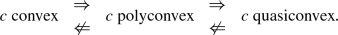
• (i) In general

  $$\begin{aligned} c\ \text {convex }\Rightarrow \text { }c\ \text {polyconvex }\Rightarrow c\ \text {quasiconvex }\Rightarrow \text { }c\ \text {rank one convex.} \end{aligned}$$

• (ii) If $k=1,$$k=n$ or $k=n-1$ is odd, then

  $$\begin{aligned} c\ \text {convex }\Leftrightarrow \text { }c\ \text {polyconvex }\Leftrightarrow \text { }c\ \text {quasiconvex }\Leftrightarrow \text { }c\ \text {rank one convex.} \end{aligned}$$

  Moreover, if k is odd or $2k>n+1,$ then

  $$\begin{aligned} c\ \text {convex }\Leftrightarrow \text { }c\ \text {polyconvex.} \end{aligned}$$

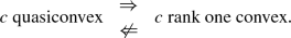
• (iii) If either $k=2$ and $n\ge 3$ or $3\le k\le n-2$ or $k=n-1\ge 4$ is even, then

  

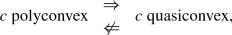
  while if $2\le k\le n-2$ (and thus $n\ge k+2\ge 4$), then

  

Remark 3.9

When $k=2,$ Theorem 3.8 yields the following:

• If $n=2,$ then

  $$\begin{aligned} c\text { convex} \quad \Leftrightarrow \quad c\text { polyconvex} \quad \Leftrightarrow \text { }c\text { quasiconvex}\quad \Leftrightarrow \quad c\text { rank one convex.} \end{aligned}$$

• If $n=3,$ then

  

• If $n\ge 4,$ then

  

We also rely on [3] and Proposition 3.3 to completely characterize the quasiaffine functions.

Lemma 3.10

Let $1\le k\le n$ and $c:\Lambda ^{k}\left( {\mathbb {R}}^{n}\right) \times \Lambda ^{k-1}\left( {\mathbb {R}}^{n}\right) \rightarrow {\mathbb {R}}.$ The following statements are then equivalent:

• (i) c is polyaffine;

• (ii) c is quasiaffine;

• (iii) c is rank one affine;

• (iv) If k is odd or $2k>n+1,$ then c is affine, i.e. there exist $c_{0}\in {\mathbb {R}},$$c_{1}\in \Lambda ^{k}\left( {\mathbb {R}}^{n}\right)$ and $d_{0}$$\in \Lambda ^{k-1}\left( {\mathbb {R}}^{n}\right)$ such that, for every $\left( \lambda ,\mu \right) \in \Lambda ^{k}\left( {\mathbb {R}}^{n}\right) \times \Lambda ^{k-1}\left( {\mathbb {R}}^{n}\right) ,$

  $$\begin{aligned} c\left( \lambda ,\mu \right) =c_{0}+\left\langle c_{1};\lambda \right\rangle +\left\langle d_{0};\mu \right\rangle , \end{aligned}$$

  while if k is even and $2k\le n+1,$ there exist $c_{0}\in {\mathbb {R}},$$d_{0}$$\in \Lambda ^{k-1}\left( {\mathbb {R}}^{n}\right) ,$$c_{r}\in \Lambda ^{kr}\left( {\mathbb {R}}^{n}\right)$ for $1\le r\le \left[ \frac{n}{k}\right] ,$$d_{s}\in \Lambda ^{ks+\left( k-1\right) }\left( {\mathbb {R}}^{n}\right)$ for $1\le s\le \left[ \frac{n-k+1}{k}\right] ,$ such that, for every $\left( \lambda ,\mu \right) \in \Lambda ^{k}\left( {\mathbb {R}}^{n}\right) \times \Lambda ^{k-1}\left( {\mathbb {R}}^{n}\right) ,$

  $$\begin{aligned} c\left( \lambda ,\mu \right) =c_{0}+\sum _{r=1}^{\left[ \frac{n}{k}\right] }\left\langle c_{r};\lambda ^{r}\right\rangle +\left\langle d_{0} ;\mu \right\rangle +\sum _{s=1}^{\left[ \frac{n-k+1}{k}\right] }\left\langle d_{s};\lambda ^{s}\wedge \mu \right\rangle \text { }. \end{aligned}$$

3.4 Existence of Minimizers

We now turn to the existence theorem for $\left( P\right)$ and $\left( P_{\mathrm {gauge}}\right)$ defined in Problems 2.3 and 2.5. We assume that $O\subset {\mathbb {R}}^{n+1}$ is a bounded open contractible set with a smooth boundary, $\widetilde{\omega }\in W^{1,s}\left( O;\Lambda ^{k-1}\left( {\mathbb {R}}^{n+1}\right) \right) ,$$c:\Lambda ^{k}\left( {\mathbb {R}} ^{n}\right) \times \Lambda ^{k-1}\left( {\mathbb {R}}^{n}\right) \rightarrow {\mathbb {R}}$ is quasiconvex, and that there exist $a_{2}\,,b_{2}>0$ such that

$$\begin{aligned} \left| c\left( \lambda ,\mu \right) \right| \le a_{2}+b_{2}\left| \left( \lambda ,\mu \right) \right| ^{s},\quad \forall \left( \lambda ,\mu \right) \in \Lambda ^{k}\left( {\mathbb {R}}^{n}\right) \times \Lambda ^{k-1}\left( {\mathbb {R}}^{n}\right) . \end{aligned}$$

Corollary 3.11

Under the above hypotheses, and if

$$\begin{aligned} \left( P\right) \quad \inf \left\{ \int _{O}c\left( f,g\right) \mathrm{d}t\,\mathrm{d}x:\left( f,g\right) \in {\mathcal {P}}^{s}\left( \widetilde{\omega }\right) \right\} \end{aligned}$$

$$\begin{aligned} \left( P_{\mathrm {gauge}}\right) \quad \inf \left\{ \int _{O}c_{\mathrm {gauge} }\left( \mathrm{d}\omega \right) \mathrm{d}t\,\mathrm{d}x:\omega \in {\mathcal {P}}_{\mathrm {gauge}} ^{s}\left( \widetilde{\omega }\right) \right\} , \end{aligned}$$

then

$$\begin{aligned} \inf \left( P\right) =\inf \left( P_{\mathrm {gauge}}\right) . \end{aligned}$$

If, in addition to the above hypotheses, there exist $a_{1}\in {\mathbb {R}},$$b_{1}>0$ such that

$$\begin{aligned} a_{1}+b_{1}\left| \left( \lambda ,\mu \right) \right| ^{s}\le c\left( \lambda ,\mu \right) ,\quad \forall \left( \lambda ,\mu \right) \in \Lambda ^{k}\left( {\mathbb {R}}^{n}\right) \times \Lambda ^{k-1}\left( {\mathbb {R}}^{n}\right) , \end{aligned}$$

then $\left( P\right)$ and $\left( P_{\mathrm {gauge}}\right)$ attain their minimum.

Proof

The fact that $\inf \left( P\right) =\inf \left( P_{\mathrm {gauge}}\right) ,$ as well as the fact that $\left( P\right)$ attains its minimum if and only if $\left( P_{\mathrm {gauge}}\right)$ attains its minimum, follow at once from Proposition 2.7. We refer to [3] for the existence of minimizers in $\left( P_{\mathrm {gauge}}\right) ,$ where Theorem 5.1 is used (to remedy the lack of compactness mentioned in the introduction). $\square$

3.5 Existence of Minimizers When O is the Cylinder

We adopt the same hypotheses (in particular, $\left( f_{0},f_{1}\right)$ are as in Definition 2.9 with $s=2$) and notations as in Subsection 2.4. In particular, $O=\left( 0,1\right) \times \Omega ,$

$$\begin{aligned} \left( P\right) \quad \inf \left\{ \int _{O}c\left( f,g\right) \mathrm{d}t\,\mathrm{d}x:\left( f,g\right) \in {\mathcal {P}}^{2}\left( f_{0},f_{1}\right) \right\} , \end{aligned}$$

and

$$\begin{aligned} \left( P_{\mathrm {gauge}}\right) \quad \inf \left\{ \int _{O}c_{\mathrm {gauge} }\left( \mathrm{d}\omega \right) \mathrm{d}t\,\mathrm{d}x:\omega \in {\mathcal {P}}_{\mathrm {gauge}} ^{2}\left( \widetilde{\omega }\right) \right\} . \end{aligned}$$

Theorem 3.12

Let $c:\Lambda ^{k}\left( {\mathbb {R}} ^{n}\right) \times \Lambda ^{k-1}\left( {\mathbb {R}}^{n}\right) \rightarrow {\mathbb {R}}$ be quasiconvex and satisfy, for some $a_{1}\,,a_{2}\in {\mathbb {R}}$ and $b_{1},b_{2}>0$,

$$\begin{aligned} a_{1}+b_{1}\left| \left( \lambda ,\mu \right) \right| ^{2}\le & {} c\left( \lambda ,\mu \right) \nonumber \\\le & {} a_{2}+b_{2}\left| \left( \lambda ,\mu \right) \right| ^{2},\quad \forall \left( \lambda ,\mu \right) \in \Lambda ^{k}\left( {\mathbb {R}}^{n}\right) \times \Lambda ^{k-1}\left( {\mathbb {R}}^{n}\right) .\nonumber \\ \end{aligned}$$

(3.2)

Then

$$\begin{aligned} \inf \left( P\right) =\inf \left( P_{\mathrm {gauge}}\right) . \end{aligned}$$

Moreover, $\left( P\right)$ and $\left( P_{\mathrm {gauge}}\right)$ attain their minimum.

Proof

The statement that $\inf \left( P\right) =\inf \left( P_{\mathrm {gauge} }\right)$ has already been proved in Theorem 2.14 .

Step 1. The proof of Theorem 2.14 reveals the following facts when $s=2$: there is a monotone sequence $\left( \epsilon _{m}\right) _{m}\subset \left( 0,1\right)$ decreasing to 0 such that by Step 2 of the proof of the theorem and by (2.26), there are

$$\begin{aligned} \left( f^{m},g^{m}\right) \in {\mathcal {P}}^{2}\left( f_{0},f_{1}\right) \end{aligned}$$

such that

$$\begin{aligned} \int _{O}c\left( f^{m},g^{m}\right) \mathrm{d}t\,\mathrm{d}x\le \inf \left( P\right) +{\frac{1}{m}\,.} \end{aligned}$$

(3.3)

If we further set $h^{m}:=f^{m}-\mathrm{d}x^{0}\wedge g^{m},$ then using Step 4 of the proof of Theorem 2.14, we have

$$\begin{aligned} \left\{ \begin{array}[c]{cl} \mathrm{d}h^{m}=0 &{}\quad \text {in }O_{{\epsilon _{m}}}\\ \nu _{\epsilon _{m}}\wedge h^{m}=\nu _{\epsilon _{m}}\wedge \mathrm{d}\widetilde{\omega } &{}\quad \text {on}\;\partial O_{{\epsilon _{m}}}\,. \end{array} \right. \end{aligned}$$

This, thanks to Theorem 7.2 [6], provides us with

$$\begin{aligned} \overline{\omega }^{m}\in W^{1,2}\left( O_{\epsilon _{m}},\Lambda ^{k-1}\left( {\mathbb {R}}^{n+1}\right) \right) \end{aligned}$$

such that

$$\begin{aligned} \left\{ \begin{array}[c]{cl} \mathrm{d}\overline{\omega }^{m}=f^{m}-\mathrm{d}x^{0}\wedge g^{m} &{}\quad \text {in }O_{{\epsilon _{m}} }\\ \delta \overline{\omega }^{m}=0 &{}\quad \text {in }O_{{\epsilon _{m}}}\\ \nu _{\epsilon _{m}}\wedge \overline{\omega }^{m}=\nu _{\epsilon _{m}} \wedge \widetilde{\omega } &{}\quad \text {on}\;\partial O_{{\epsilon _{m}}}\,. \end{array} \right. \end{aligned}$$

(3.4)

Step 2. The first inequality in (3.2), together with (3.3), implies

$$\begin{aligned} \left\| f^{m}\right\| _{L^{2}\left( O\right) }^{2}+\left\| g^{m}\right\| _{L^{2}\left( O\right) }^{2}\le {\frac{1}{b_{1}}}\left( {\frac{1}{m}}+\inf \left( P\right) -a_{1}\left| O\right| \right) . \end{aligned}$$

(3.5)

Passing to a subsequence, if necessary, we may conclude that $\left( f^{m},g^{m}\right) _{m}$ converges weakly in $L^{2}\left( O\right)$ to some $\left( f,g\right)$, which must satisfy

$$\begin{aligned} \left( f,g\right) \in {\mathcal {P}}^{2}\left( f_{0},f_{1}\right) . \end{aligned}$$

(3.6)

Thanks to (3.4), we use Theorem 8 in [7] (recall that $O_{\epsilon _{m}}$ is smooth and convex) to infer that

$$\begin{aligned} \left\| \nabla \overline{\omega }^{m}-\nabla \widetilde{\omega }\right\| _{L^{2}\left( O_{\epsilon _{m}}\right) }^{2}\le \left\| f^{m}-\mathrm{d}x^{0}\wedge g^{m}-\mathrm{d}\widetilde{\omega }\right\| _{L^{2}\left( O_{\epsilon _{m}}\right) }^{2}+\left\| \delta \widetilde{\omega }\right\| _{L^{2}\left( O_{\epsilon _{m}}\right) }^{2}\,. \end{aligned}$$

(3.7)

We combine (3.5) and (3.7) to obtain a constant $C_{*}>0$ independent of m such that

$$\begin{aligned} \left\| \nabla \overline{\omega }^{m}\right\| _{L^{2}\left( O_{\epsilon _{m}}\right) }\le C_{*}\,. \end{aligned}$$

(3.8)

For $\delta >0$ and $\epsilon _{m}\in \left( 0,\delta \right)$ (note that then $O_{\delta }\subset O_{\epsilon _{m}}$), we define for $\left( t,x\right) \in O_{\delta }\,,$

$$\begin{aligned} \overline{\omega }_{\delta }^{m}\left( t,x\right) :=\overline{\omega } ^{m}-{\frac{1}{\left| O_{\delta }\right| }}\int _{O_{\delta }} \overline{\omega }^{m}\left( s,y\right) \mathrm{d}s\,\mathrm{d}y. \end{aligned}$$

Invoking the Poincaré Wirtinger inequality, we obtain a constant $C_{\delta }$ which depends only on $\Omega _{\delta }$ (but independent of m) such that

$$\begin{aligned} \left\| \overline{\omega }_{\delta }^{m}\right\| _{W^{1,2}\left( O_{\delta }\right) }\le C_{\delta }\left\| \nabla \overline{\omega }_{\delta }^{m}\right\| _{L^{2}\left( O_{\delta }\right) }=C_{\delta }\left\| \nabla \overline{\omega }^{m}\right\| _{L^{2}\left( O_{\delta }\right) }\le C_{*}C_{\delta }\,. \end{aligned}$$

(3.9)

By (3.4), we have

$$\begin{aligned} \mathrm{d}\overline{\omega }_{\delta }^{m}=f^{m}-\mathrm{d}x^{0}\wedge g^{m}\quad \text {on }O_{\delta }\,. \end{aligned}$$

(3.10)

From (3.9), we find that there exists $\overline{\omega }_{\delta }\in W^{1,2}\left( O_{\delta };\Lambda ^{k-1}\left( {\mathbb {R}} ^{n+1}\right) \right)$ such that, up to a subsequence, $\left( \overline{\omega }_{\delta }^{m}\right) _{m}\rightharpoonup \overline{\omega }_{\delta }$ in $W^{1,2}\left( O_{\delta };\Lambda ^{k-1}\left( {\mathbb {R}} ^{n+1}\right) \right) .$ By (3.10), we get

$$\begin{aligned} \mathrm{d}\overline{\omega }_{\delta }=f-\mathrm{d}x^{0}\wedge g\quad \text {on }O_{\delta }\,. \end{aligned}$$

(3.11)

Since by (3.2) $c-a_{1}\ge 0,$ replacing c by $c-a_{1}\,,$ if necessary, we may assume, without loss of generality, that $c\ge 0.$ We use first this fact and then (3.10) to obtain

$$\begin{aligned}&\liminf _{m\rightarrow \infty }\int _{O}c\left( f^{m},g^{m}\right) \mathrm{d}t\,\mathrm{d}x\ge \liminf _{m\rightarrow \infty }\int _{O_{\delta }}c\left( f^{m} ,g^{m}\right) \mathrm{d}t\,\mathrm{d}x\\&\quad =\liminf _{m\rightarrow \infty }\int _{O_{\delta } }c_{\mathrm {gauge}}\left( \mathrm{d}\overline{\omega }_{\delta }^{m}\right) \mathrm{d}t\,\mathrm{d}x. \end{aligned}$$

This, together with the quasiconvexity of c,  the fact that $\left( \overline{\omega }_{\delta }^{m}\right) _{m}\rightharpoonup \overline{\omega }_{\delta }$ in $W^{1,2}\left( O_{\delta };\Lambda ^{k-1}\left( {\mathbb {R}} ^{n+1}\right) \right)$, and (3.11), implies

$$\begin{aligned}&\liminf _{m\rightarrow \infty }\int _{O}c\left( f^{m},g^{m}\right) \mathrm{d}t\,\mathrm{d}x\ge \int _{O_{\delta }}c_{\mathrm {gauge}}\left( d\overline{\omega }_{\delta }\right) \mathrm{d}t\,\mathrm{d}x\\&\quad =\int _{O_{\delta }}c\left( f,g\right) \mathrm{d}t\,\mathrm{d}x. \end{aligned}$$

We let $\delta$ tend to 1 and use the monotone convergence theorem to obtain

$$\begin{aligned} \liminf _{m\rightarrow \infty }\int _{O}c\left( f^{m},g^{m}\right) \mathrm{d}t\,\mathrm{d}x\ge \int _{O}c\left( f,g\right) \mathrm{d}t\,\mathrm{d}x. \end{aligned}$$

We combine this with (3.3) to infer that

$$\begin{aligned} \int _{O}c\left( f,g\right) \mathrm{d}t\,\mathrm{d}x=\inf \left( P\right) . \end{aligned}$$

This concludes the proof of the theorem. $\quad \square$

3.6 An Important Example for Applications

As mentioned in the introduction, the actions which motivate this manuscript include those which may be interpreted as kinetic energy functionals of physical systems of particles. In the sequel, we assume that $k=2$ and $n=2m$ is even and $s\ge 1.$

Given a path of symplectic forms $f\in C^{\infty }\left( \left[ 0,1\right] ;C_{0}^{\infty }\left( \overline{\Omega },\Lambda ^{2}\left( {\mathbb {R}}^{n}\right) \right) \right)$ (i.e. $d_{x}f=0$ and $f^{m}\ne 0$) and a vector field ${{\mathbf {v}}}\in C_{0}^{\infty }\left( \left[ 0,1\right] \times \Omega ;{\mathbb {R}}^{n}\right)$ such that

$$\begin{aligned} \partial _{t}f+{\mathcal {L}}_{{{\mathbf {v}}}}f=0, \end{aligned}$$

define the generalized kinetic energy functional

$$\begin{aligned} {\mathcal {E}}_{s}\left( f,{{\mathbf {v}}}\right) =\int _{\left( 0,1\right) \times \Omega }{\frac{1}{2}}\left| {{\mathbf {v}}}\right| ^{s}\varrho \,\mathrm{d}t, \end{aligned}$$

where $\varrho =f^{m}.$ Note that $\varrho$ satisfies the continuity equation

$$\begin{aligned} \partial _{t}\varrho +\nabla _{x}\cdot \left( \varrho \,{{\mathbf {v}}}\right) =0. \end{aligned}$$

Setting ${\mathbf {v=}}\sum _{i=1}^{n}{{\mathbf {v}}}_{i}{\mathbf {\,}}\mathrm{d}x^{i},$

$$\begin{aligned} g={{\mathbf {v}}}\,\lrcorner \,f,\quad f_{0}=f\left( 0,\cdot \right) ,\quad f_{1}=f\left( 1,\cdot \right) , \end{aligned}$$

(3.12)

we have that $\left( f,g\right) \in {\mathcal {P}}^{s}(f_{0},f_{1}).$ The first identity in (3.12) yields (since $f^{m}\ne 0$) ${{\mathbf {v}} }=g\,\lrcorner \,f^{-1}$, and so

$$\begin{aligned} \left| {{\mathbf {v}}}\right| ^{s}=\left| g\,\lrcorner \,f^{-1} \right| ^{s}. \end{aligned}$$

Therefore, the generalized kinetic energy functional is

$$\begin{aligned} {\mathcal {E}}_{s}\left( f,{{\mathbf {v}}}\right) =\int _{\left( 0,1\right) \times \Omega }{\frac{1}{2}}\left| g\,\lrcorner \,f^{-1}\right| ^{s} f^{m}\mathrm{d}t. \end{aligned}$$

As announced in the introduction, we show in the next proposition that, written in terms of $\left( f,g\right) ,$${\mathcal {E}}_{s}$ has a polyconvex integrand (we do not speak of quasiconvexity, because the function below can take the value $+\infty$).

Proposition 3.13

• (i) For any $\lambda \in \Lambda ^{2}\left( {\mathbb {R}}^{n}\right)$ and $\mu \in \Lambda ^{1}\left( {\mathbb {R}}^{n}\right) ,$ we have that

  $$\begin{aligned} \left( *\lambda ^{m}\right) \mu =m\left( \mu \,\lrcorner \,\lambda \right) \,\lrcorner \,\left( *\lambda ^{m-1}\right) . \end{aligned}$$

  In particular, if $*\lambda ^{m}\ne 0$, and setting $\lambda ^{-1}=\frac{m}{*\lambda ^{m}}\left( *\lambda ^{m-1}\right) ,$ then

  $$\begin{aligned} \mu \,\lrcorner \,\lambda =\widetilde{\mu }\quad \Leftrightarrow \quad \widetilde{\mu }\,\lrcorner \,\lambda ^{-1}=\mu . \end{aligned}$$

• (ii) For any $\epsilon \ge 0,$ the cost ${c}_{\epsilon }:\Lambda ^{2}\left( {\mathbb {R}}^{n}\right) \times \Lambda ^{1}\left( {\mathbb {R}} ^{n}\right) \rightarrow {\mathbb {R}}\cup \left\{ +\infty \right\}$ defined as

  $$\begin{aligned} {c}_{\epsilon }\left( \lambda ,\mu \right) =\left\{ \begin{array}[c]{cl} \left| \mu \,\lrcorner \,\lambda ^{-1}\right| ^{s}\left( *\lambda ^{m}\right) &{} \text {if }*\lambda ^{m}>\epsilon \\ +\infty &{} \text {otherwise} \end{array} \right. \end{aligned}$$

  is polyconvex.

Proof

(i) Appealing to Proposition 2.16 in [6], we can write

$$\begin{aligned} \left( *\lambda ^{m}\right) \mu= & {} -\left[ *\left( \mu \,\lrcorner \,\lambda ^{m}\right) \right] \\= & {} -\left[ *\left[ m\left( \mu \,\lrcorner \,\lambda \right) \wedge \lambda ^{m-1}\right] \right] =m\left[ \left( \mu \,\lrcorner \,\lambda \right) \,\lrcorner \,\left( *\lambda ^{m-1}\right) \right] , \end{aligned}$$

which establishes (i).

(ii) Step 1. Let ${\gamma }_{\epsilon }:\Lambda ^{1}\left( {\mathbb {R}}^{n}\right) \times {\mathbb {R}}\rightarrow {\mathbb {R}}\cup \left\{ +\infty \right\}$ be defined as

$$\begin{aligned} {\gamma }_{\epsilon }\left( x,y\right) =\left\{ \begin{array}[c]{cl} \frac{\left| x\right| ^{s}}{y^{s-1}} &{} \text {if }y>\epsilon \\ +\infty &{} \text {otherwise} \end{array} \right. \end{aligned}$$

(if $s=1,$ replace $\left| x\right| ^{s}/y^{s-1}$ by $\left| x\right|$). Note that ${\gamma }_{\epsilon }$ is convex.

Step 2. According to (i), we can write

$$\begin{aligned} \left| \mu \,\lrcorner \,\lambda ^{-1}\right| ^{s}\left( *\lambda ^{m}\right) =\left| \mu \,\lrcorner \,\left( \frac{m}{*\lambda ^{m} }\left( *\lambda ^{m-1}\right) \right) \right| ^{s}\left( *\lambda ^{m}\right) =m^{s}\,\frac{\left| \lambda ^{m-1}\wedge \mu \right| ^{s}}{\left( *\lambda ^{m}\right) ^{s-1}}\,. \end{aligned}$$

We observe that if we set $e=\mathrm{d}x^{1}\wedge \cdots \wedge \mathrm{d}x^{n},$ then $*\lambda ^{m}=\left\langle e;\lambda ^{m}\right\rangle$, and thus

$$\begin{aligned} c_{\epsilon }\left( \lambda ,\mu \right) =m^{s}\,\gamma _{\epsilon }\left( \lambda ^{m-1}\wedge \mu ,\left\langle e;\lambda ^{m}\right\rangle \right) . \end{aligned}$$

The function $c_{\epsilon }$ is therefore expressed as a convex function $\gamma _{\epsilon }$ whose arguments are quasiaffine functions (namely $\lambda ^{m-1}\wedge \mu$ and $\left\langle e;\lambda ^{m}\right\rangle$) according to Lemma 3.10, and hence $c_{\epsilon }$ is, by definition, polyconvex. $\quad \square$

4 Quasiconvex Envelope and the Relaxation Theorem

4.1 The Quasiconvex Envelope

As in the classical case [8], we define an operator $c\mapsto Q\left[ c\right]$ which associates to any cost function a quasiconvex cost function which is its envelope.

Definition 4.1

The quasiconvex envelope of $c:\Lambda ^{k}\left( {\mathbb {R}}^{n}\right) \times \Lambda ^{k-1}\left( {\mathbb {R}}^{n}\right) \rightarrow {\mathbb {R}}$ is the largest quasiconvex function $Q\left[ c\right] :\Lambda ^{k}\left( {\mathbb {R}}^{n}\right) \times \Lambda ^{k-1}\left( {\mathbb {R}}^{n}\right) \rightarrow {\mathbb {R}}$ which lies below c,  i.e.

$$\begin{aligned} Q\left[ c\right] =\sup \left\{ g:g\le c\text { and }g\text { quasiconvex} \right\} . \end{aligned}$$

Remark 4.2

• (i) For $c_{\mathrm {gauge}}:\Lambda ^{k}\left( {\mathbb {R}}^{n+1}\right) \rightarrow {\mathbb {R}}$, as in Problem 2.5 (see also Proposition 3.3), we define the quasiconvex envelope as

  $$\begin{aligned} Q\left[ c_{\mathrm {gauge}}\right] =\sup \left\{ g:g\le c_{\mathrm {gauge} }\text { and }g\text { is ext. quasiconvex}\right\} . \end{aligned}$$

• (ii) If we set

  $$\begin{aligned} C_{\mathrm {gauge}}=c_{\mathrm {gauge}}\circ \pi :{\mathbb {R}}^{\genfrac(){0.0pt}1{n+1}{k-1}\times \left( n+1\right) }\rightarrow {\mathbb {R}} \end{aligned}$$

  (cf. Theorem 3.7), then $Q\left[ C_{\mathrm {gauge}}\right]$ is the quasiconvex envelope in the classical sense.

The next theorem provides a representation formula for $Q\left[ c\right]$ in terms of c.

Theorem 4.3

Let $c,h:\Lambda ^{k}\left( {\mathbb {R}}^{n}\right) \times \Lambda ^{k-1}\left( {\mathbb {R}}^{n}\right) \rightarrow {\mathbb {R}}$ be Borel measurable and locally bounded with h quasiconvex below c (i.e. $h\le c$). Let $c_{\mathrm {gauge}}\,,$$Q\left[ c_{\mathrm {gauge}}\right] ,$$C_{\mathrm {gauge}}$ and $Q\left[ C_{\mathrm {gauge}}\right]$ be as in Remark 4.2. Then

$$\begin{aligned} Q\left[ c\right] =Q\left[ c_{\mathrm {gauge}}\right] \quad \text {and}\quad Q\left[ C_{\mathrm {gauge}}\right] =Q\left[ c_{\mathrm {gauge}}\right] \circ \pi . \end{aligned}$$

Moreover, for every $\left( \lambda ,\mu \right) \in \Lambda ^{k}\left( {\mathbb {R}}^{n}\right) \times \Lambda ^{k-1}\left( {\mathbb {R}}^{n}\right) ,$

$$\begin{aligned}&Q\left[ c\right] \left( \lambda ,\mu \right) \\&\quad =\inf _{\begin{array}{c} \varphi \in W_{0}^{1,\infty }\left( O;\Lambda ^{k-1}\left( {\mathbb {R}}^{n}\right) \right) \\ \psi \in W_{0}^{1,\infty }\left( O;\Lambda ^{k-2}\left( {\mathbb {R}} ^{n}\right) \right) \end{array}}\left\{ \frac{1}{{\text {meas}}\,O}\int _{O}c\left( \lambda +d_{x}\varphi ,\mu -\partial _{t}\varphi +d_{x}\psi \right) \mathrm{d}t\,\mathrm{d}x\right\} , \end{aligned}$$

where $O\subset {\mathbb {R}}^{n+1}$ is a bounded open set. In particular, the infimum in the formula is independent of the choice of O and can be taken, for example, as $\left( 0,1\right) ^{n+1}.$

Proof

The identity $Q\left[ c\right] =Q\left[ c_{\mathrm {gauge}}\right]$ has to be understood as

$$\begin{aligned} Q\left[ c_{\mathrm {gauge}}\right] \left( \xi \right) =Q\left[ c\right] \left( \pi _{x}\left( \xi \right) ,-\pi _{0}\left( \xi \right) \right) ,\quad \forall \,\xi \in \Lambda ^{k}\left( {\mathbb {R}}^{n+1}\right) , \end{aligned}$$

and it follows at once from the definition of $c_{\mathrm {gauge}}$ and Theorem 3.7. Next, let

$$\begin{aligned} \Xi \in {\mathbb {R}}^{\genfrac(){0.0pt}1{n+1}{k-1}\times \left( n+1\right) }\quad \text {and}\quad \xi =\pi \left( \Xi \right) \in \Lambda ^{k}\left( {\mathbb {R}} ^{n+1}\right) , \end{aligned}$$

and set

$$\begin{aligned} {\widetilde{c}}\left( \xi \right) =\inf \left\{ \frac{1}{{\text {meas}}\,O}\int _{O}c_{\mathrm {gauge}}\left( \xi +\mathrm{d}\omega \right) \mathrm{d}t\,\mathrm{d}x:\omega \in W_{0}^{1,\infty }\left( O;\Lambda ^{k-1}\left( {\mathbb {R}}^{n+1}\right) \right) \right\} . \end{aligned}$$

If we denote ${\widetilde{C}}={\widetilde{c}}\circ \pi ,$ then

$$\begin{aligned} {\widetilde{c}}\left( \xi \right) ={\widetilde{c}}\circ \pi \left( \Xi \right) ={\widetilde{C}}\left( \Xi \right) . \end{aligned}$$

It follows by the classical result (see [8] and [10]) that, with the notations of Remark 4.2,

$$\begin{aligned}&Q\left[ C_{\mathrm {gauge}}\right] \left( \Xi \right) \\&\quad =\inf \left\{ \frac{1}{{\text {meas}}\,O}\int _{O}C_{\mathrm {gauge}}\left( \Xi +\nabla \Phi \right) \mathrm{d}t\,\mathrm{d}x:\Phi \in W_{0}^{1,\infty }\left( O;{\mathbb {R}}^{\genfrac(){0.0pt}1{n+1}{k-1}}\right) \right\} \end{aligned}$$

(and also that the formula is independent of the set O). We therefore deduce that $Q\left[ C_{\mathrm {gauge}}\right] ={\widetilde{C}}={\widetilde{c}}\circ \pi .$ Thus ${\widetilde{C}}$ is quasiconvex and, by Theorem 3.7, ${\widetilde{c}}$ is ext. quasiconvex. We have hence obtained that ${\widetilde{c}}\le Q\left[ c_{\mathrm {gauge} }\right] .$ Using Theorem 3.7 again, we infer that $Q\left[ c_{\mathrm {gauge}}\right] \circ \pi$ is quasiconvex. Summarizing these results, we have shown that

$$\begin{aligned} Q\left[ c_{\mathrm {gauge}}\right] \circ \pi \le Q\left[ C_{\mathrm {gauge} }\right] ={\widetilde{C}}={\widetilde{c}}\circ \pi , \end{aligned}$$

and thus $Q\left[ c_{\mathrm {gauge}}\right] \le {\widetilde{c}}.$ We have therefore proved that

$$\begin{aligned} Q\left[ c_{\mathrm {gauge}}\right] ={\widetilde{c}}\quad \text {and}\quad Q\left[ C_{\mathrm {gauge}}\right] =Q\left[ c_{\mathrm {gauge}}\right] \circ \pi ={\widetilde{c}}\circ \pi , \end{aligned}$$

and the theorem is established. $\quad \square$

Remark 4.4

In view of Theorem 3.8 (ii), when $k=1$ (and hence $\psi \equiv 0$) or $k=n,$ then $Q\left[ c\right] =c^{**}.$ In general, $Q\left[ c\right] \ge c^{**},$ but it usually happens (particularly when $k=2$) that $Q\left[ c\right] >c^{**}.$

4.2 The Relaxation Theorem

We assume below that $O\subset {\mathbb {R}}^{n+1}$ is a bounded open contractible set with smooth boundary, $\widetilde{\omega }\in W^{1,s}\left( O;\Lambda ^{k-1}\left( {\mathbb {R}}^{n+1}\right) \right) ,$$h,c:\Lambda ^{k}\left( {\mathbb {R}}^{n}\right) \times \Lambda ^{k-1}\left( {\mathbb {R}}^{n}\right) \rightarrow {\mathbb {R}}$ with h quasiconvex and there exist $a_{2}\,,b_{2}>0$ such that

$$\begin{aligned} h\left( \lambda ,\mu \right) \le c\left( \lambda ,\mu \right) \le a_{2}+b_{2}\left| \left( \lambda ,\mu \right) \right| ^{s} ,\quad \forall \left( \lambda ,\mu \right) \in \Lambda ^{k}\left( {\mathbb {R}} ^{n}\right) \times \Lambda ^{k-1}\left( {\mathbb {R}}^{n}\right) . \end{aligned}$$

Theorem 4.5

(Relaxation theorem). Let $Q\left[ c\right]$ be the quasiconvex envelope of c and

$$\begin{aligned}&\left( P\right) \quad \inf \left\{ \int _{O}c\left( f,g\right) \mathrm{d}t\,\mathrm{d}x:\left( f,g\right) \in {\mathcal {P}}^{s}\left( \widetilde{\omega }\right) \right\} \\&\left( QP\right) \quad \inf \left\{ \int _{O}Q\left[ c\right] \left( f,g\right) \mathrm{d}t\,\mathrm{d}x:\left( f,g\right) \in {\mathcal {P}}^{s}\left( \widetilde{\omega }\right) \right\} . \end{aligned}$$

Then

$$\begin{aligned} \inf \left( P\right) =\inf \left( QP\right) . \end{aligned}$$

Moreover, if there exists $a_{1}\in {\mathbb {R}},$$b_{1}>0$ such that

$$\begin{aligned} a_{1}+b_{1}\left| \left( \lambda ,\mu \right) \right| ^{s}\le c\left( \lambda ,\mu \right) ,\quad \forall \left( \lambda ,\mu \right) \in \Lambda ^{k}\left( {\mathbb {R}}^{n}\right) \times \Lambda ^{k-1}\left( {\mathbb {R}}^{n}\right) , \end{aligned}$$

(4.1)

then $\left( QP\right)$ attains its minimum and, for every $\left( f,g\right) \in {\mathcal {P}}^{s}\left( \widetilde{\omega }\right) ,$ there exists a sequence $\left\{ \left( f^{N},g^{N}\right) \right\} _{N=1}^{\infty }\subset {\mathcal {P}}^{s}\left( \widetilde{\omega }\right)$ such that, as $N\rightarrow \infty ,$

$$\begin{aligned}&\left( f^{N},g^{N}\right) \rightharpoonup \left( f,g\right) \quad \text {weakly in }L^{s}\left( O;\Lambda ^{k}\left( {\mathbb {R}}^{n}\right) \times \Lambda ^{k-1}\left( {\mathbb {R}}^{n}\right) \right) \\&\int _{O}c\left( f^{N},g^{N}\right) \mathrm{d}t\,\mathrm{d}x\rightarrow \int _{O}Q\left[ c\right] \left( f,g\right) \mathrm{d}t\,\mathrm{d}x. \end{aligned}$$

Remark 4.6

Combining the above Theorem 4.5 with Corollary 3.11, we also have

$$\begin{aligned} \inf \left( P\right) =\inf \left( QP\right) =\inf \left( P_{\mathrm {gauge} }\right) =\inf \left( \left( QP\right) _{\mathrm {gauge}}\right) , \end{aligned}$$

where

$$\begin{aligned}&\left( P_{\mathrm {gauge}}\right) \quad \inf \left\{ \int _{O}c_{\mathrm {gauge} }\left( \mathrm{d}\omega \right) \mathrm{d}t\,\mathrm{d}x:\omega \in {\mathcal {P}}_{\mathrm {gauge}} ^{s}\left( \widetilde{\omega }\right) \right\} \\&\left( \left( QP\right) _{\mathrm {gauge}}\right) \quad \inf \left\{ \int _{O}Q\left[ c_{\mathrm {gauge}}\right] \left( \mathrm{d}\omega \right) \mathrm{d}t\,\mathrm{d}x:\omega \in {\mathcal {P}}_{\mathrm {gauge}}^{s}\left( \widetilde{\omega }\right) \right\} . \end{aligned}$$

Proof

(Theorem 4.5). We set $C_{\mathrm {gauge}} =c_{\mathrm {gauge}}\circ \pi .$ Recall that we identified $\Lambda ^{k-1}\left( {\mathbb {R}}^{n+1}\right)$ with ${\mathbb {R}}^{\genfrac(){0.0pt}1{n+1}{k-1}}.$ Therefore, depending on the context, we write

$$\begin{aligned} \omega \in \widetilde{\omega }+W_{0}^{1,s}\left( O;\Lambda ^{k-1}\left( {\mathbb {R}}^{n+1}\right) \right) . \end{aligned}$$

Step 1. Appealing to Theorem 4.3 and Lemma 3.6 (ii), we infer the new formulations

$$\begin{aligned} \left( P_{\mathrm {gauge}}\right) \quad \inf \left\{ \int _{O}C_{\mathrm {gauge} }\left( \nabla \omega \right) :\omega \in \widetilde{\omega }+W_{0}^{1,s}\left( O;\Lambda ^{k-1}\left( {\mathbb {R}}^{n+1}\right) \right) \right\} \end{aligned}$$

$$\begin{aligned} \left( \left( QP\right) _{\mathrm {gauge}}\right) \quad \inf \left\{ \int _{O}Q\left[ C_{\mathrm {gauge}}\right] \left( \nabla \omega \right) :\omega \in \widetilde{\omega }+W_{0}^{1,s}\left( O;\Lambda ^{k-1}\left( {\mathbb {R}}^{n+1}\right) \right) \right\} . \end{aligned}$$

By the classical relaxation theorem (cf. e.g. [8] or Theorem 9.1 in [10]),

$$\begin{aligned} \inf \left( P_{\mathrm {gauge}}\right) =\inf \left( \left( QP\right) _{\mathrm {gauge}}\right) , \end{aligned}$$

which establishes the fact that $\inf \left( P\right) =\inf \left( QP\right) .$

Step 2. It remains to address the properties of minimizing sequences under the extra assumption (4.1). Let $\left( f,g\right) \in {\mathcal {P}}^{s}\left( \widetilde{\omega }\right) .$ Invoking Proposition 2.7, we find $\omega \in \widetilde{\omega }+W_{0}^{1,s}\Bigl ( \bigl (O;\Lambda ^{k-1}\left( {\mathbb {R}}^{n+1}\right) \bigr )\Bigr )$ such that

$$\begin{aligned} \left( f,g\right) =\left( \pi _{x}\left( \mathrm{d}\omega \right) ,-\pi _{0}\left( \mathrm{d}\omega \right) \right) . \end{aligned}$$

The classical duality theory (cf. e.g. Theorem 9.1 in [10]) gives that for every $\omega \in \widetilde{\omega }+W_{0}^{1,s}$, there exists $\omega ^{N}\in \widetilde{\omega }+W_{0}^{1,s}$ such that

$$\begin{aligned}&\mathrm{d}\omega ^{N}\rightharpoonup \mathrm{d}\omega \;\text {in }L^{s}\left( O;\Lambda ^{k}\left( {\mathbb {R}}^{n+1}\right) \right) \quad \text {and}\\&\quad \int _{O}C_{\mathrm {gauge}}\left( \nabla \omega ^{N}\right) \rightarrow \int _{O}Q\left[ C_{\mathrm {gauge}}\right] \left( \nabla \omega \right) . \end{aligned}$$

Setting $\left( f^{N},g^{N}\right) =\left( \pi _{x}\left( \mathrm{d}\omega ^{N}\right) ,-\pi _{0}\left( \mathrm{d}\omega ^{N}\right) \right) ,$ we have indeed established the theorem. $\quad \square$

Appendix: Systems of the Type \(\left( d,\delta \right) \) and Poincaré lemma

We start with a classical theorem which can be found, for instance, in [6] Theorem 7.2 or Schwarz [22].

Theorem 5.1

Let $1\le k\le n$ be an integer, $1<s<\infty$ and $\Omega \subset {\mathbb {R}}^{n}$ be a bounded open smooth contractible set with exterior unit normal $\nu .$ Then the following statements are equivalent:

• (i) $f\in L^{s}\left( \Omega ;\Lambda ^{k}\right) ,$$g\in L^{s}\left( \Omega ;\Lambda ^{k-2}\right)$ and $F_{0}\in W^{1,s}\left( \Omega ;\Lambda ^{k-1}\right)$ satisfy

  $$\begin{aligned} \left\{ \begin{array}[c]{cl} {\displaystyle \int _{\Omega }} \langle f;\delta \varphi \rangle - {\displaystyle \int _{\partial \Omega }} \langle \nu \wedge F_{0};\delta \varphi \rangle =0,\;\forall \,\varphi \in C^{\infty }\left( \overline{\Omega };\Lambda ^{k+1}\right) &{} \text {if }1\le k\le n-1\\ {\displaystyle \int _{\Omega }} f= {\displaystyle \int _{\partial \Omega }} \nu \wedge F_{0} &{} \text {if }k=n \end{array} \right. \end{aligned}$$
  $$\begin{aligned} {\displaystyle \int _{\Omega }} \langle g;\mathrm{d}\varphi \rangle =0,\;\forall \,\varphi \in C_{0}^{\infty }\left( \Omega ;\Lambda ^{k-3}\right) ; \end{aligned}$$

• (ii) There exists $F\in W^{1,s}(\Omega ;\Lambda ^{k-1})$ such that

  $$\begin{aligned} \left\{ \begin{array}[c]{cl} \mathrm{d}F=f\quad \text {and}\quad \delta F=g &{} \text {in }\Omega \\ \nu \wedge F=\nu \wedge F_{0} &{} \text {on }\partial \Omega . \end{array} \right. \end{aligned}$$

Remark 5.2

• (i) If $1\le k\le n-1,$ then the conditions in (i) just mean, in the weak sense, that

  $$\begin{aligned} \left[ \mathrm{d}F=0\text { and }\delta g=0\;\text {in }\Omega \right] \text { and }\left[ \nu \wedge f=\nu \wedge \mathrm{d}F_{0}\;\text {on }\partial \Omega \right] . \end{aligned}$$

• (ii) If $k=1,$ then the terms $\delta F$ and g are not present, while if $k=2,$ then $\delta g=0$ automatically.

The preceding theorem leads to the Poincaré lemma (cf., for example, Theorem 8.16 in [6]).

Theorem 5.3

(Poincaré Lemma). Let $1\le k\le n$ be an integer, $1<s<\infty$ and $\Omega \subset {\mathbb {R}}^{n}$ be a bounded open smooth contractible set with exterior unit normal $\nu .$ Then the following statements are equivalent:

• (i) $f\in L^{s}\left( \Omega ;\Lambda ^{k}\right)$ and $F_{0}\in W^{1,s}\left( \Omega ;\Lambda ^{k-1}\right)$ satisfy

  $$\begin{aligned} \left\{ \begin{array}[c]{cl} {\displaystyle \int _{\Omega }} \langle f;\delta \varphi \rangle - {\displaystyle \int _{\partial \Omega }} \langle \nu \wedge F_{0};\delta \varphi \rangle =0,\;\forall \,\varphi \in C^{\infty }\left( \overline{\Omega };\Lambda ^{k+1}\right) &{} \text {if }1\le k\le n-1\\ {\displaystyle \int _{\Omega }} f= {\displaystyle \int _{\partial \Omega }} \nu \wedge F_{0} &{} \text {if }k=n; \end{array} \right. \end{aligned}$$

• (ii) There exists $F\in W^{1,s}(\Omega ;\Lambda ^{k-1})\$such that

  $$\begin{aligned} \left\{ \begin{array}[c]{cl} \mathrm{d}F=f &{}\quad \text {in }\Omega \\ F=F_{0} &{}\quad \text {on }\partial \Omega . \end{array} \right. \end{aligned}$$

References

Ambrosio, L., Gigli, N., Savaré, G.: Gradient flows in metric spaces and the Wasserstein spaces of probability measures, Lectures in Mathematics, ETH Zürich, Birkhäuser 2005
Ball, J.M.: Convexity conditions and existence theorems in nonlinear elasticity. Archi. Rat. Mech. Anal. 64, 337–403, 1977
Bandyopadhyay, S., Dacorogna, B., Sil, S.: Calculus of variations with differential forms. J. Eur. Math. Soc. 17, 1009–1039, 2015
Bandyopadhyay, S., Sil, S.: Exterior convexity and calculus of variations with differential forms. ESAIM Control Optim. Calc. Var. 22, 338–354, 2016
Brenier, Y.: Polar factorization and monotone rearrangement of vector-valued functions. Commun. Pure Appl. Math. 44, 375–417, 1991
Csato, G., Dacorogna, B., Kneuss, O.: The Pullback Equation for Differential Forms. Birkhäuser, Basel 2012
Csato, G., Dacorogna, B., Sil, S.: On the best constant in Gaffney inequality. J. Funct. Anal. 274, 461–503, 2018
Dacorogna, B.: Quasiconvexity and relaxation of nonconvex variational problems. J. Funct. Anal. 46, 102–118, 1982
Dacorogna, B.: Weak Continuity and Weak Lower Semicontinuity of Non-linear Functionals. Springer, Berlin 1982
Dacorogna, B.: Direct Methods in the Calculus of Variations, 2nd edn. Springer, Berlin 2007
Dacorogna, B., Gangbo W.: Transportation of closed differential forms with non-homogeneous convex costs, to appear in Calc. Var. Partial Differ. Equ. 2018
Dacorogna, B., Gangbo, W., Kneuss, O.: Optimal transport of closed differential forms for convex costs. C. R. Math. Acad. Sci. Paris Ser. I 353, 1099–1104, 2015
Dacorogna, B., Gangbo, W., Kneuss O.: Symplectic factorization, Darboux theorem and ellipticity. Ann. Inst. H. Poincaré Anal. Non Linéaire 2018
Evans, L.C.: Quasiconvexity and partial regularity in the calculus of variations. Arch. Rat. Mech. Anal. 95, 227–252, 1986
Evans, L.C., Gangbo, W.: Differential equations methods for the Monge–Kantorovich mass transfer problem. Mem. AMS 137(653), 1–66, 1999
Fonseca, I., Müller, S.: A-quasiconvexity, lower semicontinuity and Young measures. SIAM J. Math. Anal. 30, 1355–1390, 1999
Gangbo, W.: An elementary proof of the polar decomposition of vector-valued functions. Arch. Rat. Mech. Anal. 128, 380–399, 1995
Gangbo, W., McCann, R.: Optimal maps in Monge’s mass transport problem. C. R. Math. Acad. Sci. Paris Ser. I 321, 1653–1658, 1995
Gangbo, W., McCann, R.: The geometry of optimal transport. Acta Math. 177, 113–161, 1996
Gangbo, W., Van der Putten, R.: Uniqueness of equilibrium configurations in solid crystals. SIAM J. Math. Anal. 32, 465–492, 2000
Morrey, C.B.: Multiple Integrals in the Calculus of Variations. Springer, Berlin 1966
Schwarz, G.: Hodge Decomposition—A Method for Solving Boundary Value Problems, Lecture Notes in Math. 1607, Springer, Berlin 1995
Sil, S.: Calculus of variations: a differential form approach. Adv. Calc. Var. 12, 57, 2018
Silhavy, M.: Polyconvexity for functions of a system of closed differential forms. Calc. Var. Partial Differ. Equ. 57, 26, 2018
Acknowledgements
The authors wish to thank O. Kneuss and S. Sil for interesting discussions. We also thank the two anonymous referees for their very useful comments. WG acknowledges NSF support through contract DMS–17 00 202.
Author information
Authors and Affiliations
Corresponding author
Additional information
Communicated by I. Fonseca
Publisher's Note
Springer Nature remains neutral with regard to jurisdictional claims in published maps and institutional affiliations.