
Abstract
This paper develops a general equilibrium geographical economics model, which uses matching frictions on the labor market to generate regional unemployment disparities alongside the usual core-periphery pattern of industrial agglomeration. In the model, regional wage differentials do not only influence migration decisions of mobile workers, but also affect the bargaining process on local labor markets, leading to differences in vacancies and unemployment as well. In a setting with two regions, both higher or lower unemployment rates in the core region are possible equilibrium outcomes, depending on transport costs and the elasticity of substitution. Stylized facts suggest that both patterns are of empirical relevance.
1 Introduction
The simultaneous existence of densely and sparsely populated areas is a well-known empirical phenomenon. New economic geography (NEG) models use a combination of increasing returns, transport costs, and factor mobility to describe the formation and persistence of agglomerations as an endogenous process rather than a result of pure first nature differentials. They recognize the optimizing behavior of economic agents as the rationale behind regional patterns of population and industrial density. The classical model has been proposed by Krugman (1991) and was canonized in Fujita et al. (1999). Since then, it has been varied and extended in many different ways.Footnote 1
Another empirical regularity is profound employment and/or unemployment differentials between regions, even if those regions are in close proximity and face a comparable institutional setting. It seems natural to expect that both regional patterns are driven by the same or at least closely related forces. For example, Südekum (2005) shows that, evaluated at the NUTS-2 level, densely populated European regions tend to have lower unemployment rates than peripheral ones.
In recent years, economic theorists have tried to incorporate imperfect labor markets into the NEG framework to learn more about the connection between agglomeration forces and labor market differentials.Footnote 2 There have been two main ways to attain that goal. One strand of the literature concentrates on industrial clustering while not allowing for interregional labor mobility. This assumption is appropriate if migration is considered being negligible.Footnote 3 When explicitly including unemployment,Footnote 4 the result is a negative relationship between industrial agglomeration and the local unemployment rate (see Francis 2003). As a drawback, these models cannot account for endogenous regional differentials in population densities.
The second class of models allows for regional migration. One example is the model by Südekum (2005), who introduces efficiency wages to an analytically solvable agglomeration model. This results in a stable wage curve relation that is even intensified by migration.Footnote 5 Another approach is by Epifani and Gancia (2005), who model regional unemployment by introducing search frictions to a dynamic NEG framework. In both cases, the equilibrium outcome is again higher unemployment in the periphery.Footnote 6
Yet, the empirical pattern just mentioned does not necessarily hold for more disaggregated data in a national context. For example, Table 1 presents in its first column the standardized coefficients of a regression of regional unemployment rates on log population densities for the largest European countries plus the United States and Japan in 2005.Footnote 7 It shows unemployment rates to be significantly higher in densely populated areas in West Germany, France, the United Kingdom, and the United States.Footnote 8 The correlation is also positive but not significant at the 5 %—level for Spain and Japan, where the number of territorial units is smaller.
This pattern is not new to the economic literature. The formal analysis of higher unemployment in urban compared to rural areas at least goes back to the work of Harris and Todaro (1970). It is also the decisive feature of the “spatial mismatch” literature, which emerged to explain high unemployment in the cores of US cities (see Gobillon et al. 2003, for an overview). The goal of this article is to show how such a pattern can result as an equilibrium outcome in a NEG model.
The paper introduces job search frictions into a geographical general equilibrium framework.Footnote 9 Firms seeking new workers have to bear certain costs until a vacancy can be filled. These costs are linked to the local wage level by assuming that some additional workers are needed to carry out the searching. In the model, regional wage effects created by the well-known agglomeration and dispersion forces affect expected returns in the bargaining process, thus having feedback effects on wage formation and leading to unemployment differentials. It is shown that job search costs can result in both lower or higher unemployment in agglomerations.
When transport costs are high, demand is mainly local and fierce competition in a core region drives down nominal wages thus bringing them closer to replacement benefits and increasing unemployment. This is only a long-run equilibrium as long as transport costs are not too high, which would lead to complete dispersion of economic activity. When transport costs are low, strong supply and demand linkages in the core induce a nominal wage advantage and thus a lower unemployment rate.
The remainder of the article is organized as follows. Section 2 develops the basic model. Section 3 states the short-run equilibrium conditions for the multi-region case. Section 4 shows some illustrative simulations in a two-region model, performs a sensitivity analysis, and discusses the results. Section 5 concludes.
2 The model
We assume an economy that resembles the canonical Core-Periphery model. There is a modern sector using one type of labor to produce a variety of differentiated goods under monopolistic competition and a traditional sector using another type of labor and a constant-returns technology that provides a homogenous good. While workers in the traditional sector are immobile, workers in the modern sector are free to locate in any of the economy’s \(n=1,\ldots ,N\) regions. The following results hold for each region separately. To save notation, subscripts for location will not be introduced until Sect. 3.
2.1 Trade in the labor market
The market for immobile labor is assumed to be perfectly competitive. It is only the workers and firms in the modern sector that face matching frictions. With \(L^{M}\) being the number of mobile workers, unemployment rate \(u\) and vacancy rate \(v\), the number of job matchings per unit time is given by the matching function:Footnote 10
which is increasing in its arguments, concave and homogeneous of degree 1. Introducing \(\theta \equiv v/u\) as an indicator of labor market tightness, the rate at which vacant jobs are filled can be written as \(q(\theta )=m(u/v,1)\) with \(q^{\prime }(\theta )\le 0\) and the rate at which unemployed workers are hired is \(\theta q(\theta )\). Occupied jobs get separated with probability \(\delta \), so in steady state equilibrium, it must hold that flows into and out of the pool of unemployed workers equalize, thus \(\delta (1-u)L^{M}=\theta q(\theta ) u L^{M}\). Solving for \(u\) yields the Beveridge curve:
Assuming \(\delta \) to be a model parameter independent of location, it is only differences in labor market tightness that can spur regional disparities in unemployment rates. The source of these differences will be elaborated in Sect. 2.5.
2.2 Consumers
The behavior of consumers in the model directly carries over from the standard core-periphery model like in Fujita et al. (1999). Since nothing crucial can be learned by making the consumer decision dynamic, we will assume that all income has to be spent instantly and simply stick to the well-known static formulation.Footnote 11 Consumers share a common Cobb-Douglas type utility function for goods from both sectors:
\(M\) being the composite index of consumed modern goods and A being consumption of the traditional good. \(\mu \) is a constant defining expenditure shares. The subutility \(M\) is achieved by consuming a continuum of varieties with range \(k\) where quantities are represented by \(m(i)\):Footnote 12
\(\rho \) is directly linked to the elasticity of substitution \(\sigma \) by \(\sigma \equiv 1/(1-\rho )\) and indicates love-of-variety in modern goods. If \(\rho \) rises, consumers will value variety less.
Keeping the consumers budget constraint in mind and solving the two-step cost minimization problem shows that demand for each variety can be expressed as
and demand for the traditional good as
where \(Y\) is disposable income and \(p(i)\) and \(p^{A}\) are prices of the modern and traditional goods, respectively. \(G\) is the overall price index for the modern sector. It is defined by:
2.3 Workers
Workers in the modern sector earn real wage \(w^{W}\) when employed and get real benefit payments \(z^{W}\) (measured in consumer prices) when unemployed.Footnote 13 Assuming they pay a constant tax \(t\) in both cases to finance unemployment insurance, incentives remain unchanged. The tax can thus be left out of the workers decision problem within a region.Footnote 14 With \(U\) and \(E\) as the present-discounted value of the expected income of an unemployed and employed worker, respectively, \(U\) satisfies
where \(r\) denotes the interest rate. \(rU\) can be interpreted as the reservation wage. It consists of the level of unemployment benefits plus the expected capital gain from finding a job. The value function of an employed worker is given by
The difference between real wage \(w^{W}\) and permanent income \(rE\) of the employed is due to the fact that they face the risk of losing their job and falling back into the pool of the unemployed.
2.4 Producers
The matching friction in the labor market for mobile workers arises because existing jobs get canceled with rate \(\delta \) and vacancies are costly. The value function of a vacancy for a firm shall be
where \(J\) and \(V\) are the present-discounted values of expected profit from an occupied and a vacant job, respectively. \(w^{F}\) denotes the real wage from a firm’s perspective. In steady state, the capital cost equals the rate of return on the job. The vacant job costs are assumed to be a constant fraction \(\gamma \) of the real wage. One can think of them as wages for additional employees who are not engaged in the production process, but instead in human resources.Footnote 15
Since it is profitable to create new jobs until the value of a vacancy reaches zero, we get \(V=0\) as an equilibrium condition, which leads to
In equilibrium, the expected profit from a newly filled job equals the expected costs of a vacancy.
Following Ziesemer (2005), we now introduce an increasing returns production technology for the modern sector in our model. To produce a quantity \(x\) of any variety at a given location, labor input \(\ell \) will be
with fixed costs \(F\) and the standard variable part \(c x\). The last term enters the equation because a firm always has to offer a certain number of jobs \(O\) to keep employment from falling. Since each job offer will be filled with probability \(q(\theta )\) and occupied jobs get separated with rate \(\delta \), the firms expected change of employment isFootnote 16
In steady state, \(\dot{\ell }\) will be zero. Combining (12) and (13) then yields the fraction of mobile workers who are engaged in a productive task:
This expression falls in \(\theta \), so the tighter the labor market, the higher the share of labor engaged in nonproductive search activity. Inserting (12) into (13) and using the envelope theorem, we get the transition equation
The present-discounted value of the firm’s profit is
where \(p\) is the mill price of the produced good and \(W\) denotes the nominal wage. The firm maximizes (16) with respect to the quantity produced \(x\) and the number of vacancies \(O\), and we get the familiar result that optimal price will be a markup on marginal costs:Footnote 17
Marginal costs here consist of two parts. The first term in brackets represents the current costs of new production workers, which consist of the wage and average costs until a job gets filled. The second term in brackets captures the fact that not all newly hired workers will be employed in production. \(\partial \hat{p}/ \partial \theta >0\), so that prices will rise if labor market tightness increases for a given wage level.
We can also derive an expression for the current value of the expected value of a job:
It is therefore the net return generated by a worker times the probability that a worker actually performs a productive task.
Next, we want to turn to optimal output. Current profit in (16) will be zero in equilibrium, so we get
Inspection of \(\hat{x}\) shows that optimal output falls in \(\theta \), which also implies an absolute decline in per-firm labor input in production. Labor demand is given by
and the number of firms by
The effect of \(\theta \) on per-firm labor demand and the equilibrium number of firms is ambiguous. Under certain conditions, a firm will always hire more workers in a tightening labor market, so the fall in production workforce is more than offset by rising search employment.Footnote 18 Otherwise, the derivative gets negative for low values of \(\theta \). The effect of \(\theta \) on productivity is unambiguously negative, nonetheless. Combining Eqs. (19) and (20), we get that \(\partial (\hat{x}/\hat{\ell })/\partial \theta < 0\).
The above shows that a change in labor market tightness will not only have an impact on unemployment rates, but also influence prices and the structure of production. Until now, we treated \(\theta \) as exogenous, neglecting the decision processes of workers and firms affecting job search and offers. We therefore introduce a wage bargaining process in the next section, thus endogenizing \(\theta \).
2.5 Wage bargaining
A worker and a firm will only agree on a job arrangement if their respective returns on the job, \(E\) and \(J\) outweigh their fallback positions U and V. Assume they bargain over the matching rent according to a Nash bargaining game, thus maximizing the weighted product of their net returns from the job:
where \(\beta \) is the relative bargaining power of workers. From the first-order maximization condition, we get:Footnote 19
Workers receive their reservation wage \(rU\) and a fraction \(\beta \) of the net surplus created in production. This surplus consists of \(\rho /c\), which is a markup on the average product,Footnote 20 and the reservation wage they give up. Substituting for \(rU\) in (23) and rearranging, we get:Footnote 21
In standard matching models, an equation like (24) pins down the equilibrium value of \(\theta \) as a function of constant parameters. In the remainder of the paper, we want to look at a model with multiple local labor markets, where nominal wages might differ regionally due to different levels of agglomeration. Equation (24) is an implicit function in \(W\) and \(\theta \). Inspection of the first derivatives shows that the sign of \(\partial \theta / \partial W\) is positive. Since \(\theta \) and \(u\) are negatively related (see Eq. (2)), Eq. (24) represents a negatively sloped wage curve relationship. On the labor market, high unemployment is associated with low wages.Footnote 22 But we saw in Sect. 2.4 that high unemployment (and thus low \(\theta \)) has a positive effect on firm productivity. Since it gets easier for them to hire new workers, they will put a smaller share of their resources into search efforts. For given nominal wages, this leads to lower prices and thus higher real wages. Furthermore, regional wages crucially depend on demand for local goods. Since the latter arises in all regions and not only the location where production takes place, we will now have to explicitly take the regional perspective into account.
3 Regional conditions for equilibrium
As a result of the increasing returns to scale technology, each variety of the modern goods will only be produced in a single location. We will also assume that all \(k_{n}\) varieties produced in a particular location \(n\) are symmetric. Transport costs between regions will take the “iceberg” form, so for one unit of a good produced in \(n\) to arrive at its destination \(s, T_{ns}\) units will have to be shipped.Footnote 23 So the c.i.f. price at each location is given by the transport cost weighted f.o.b. price:
Using (7), the price index at location \(s\) can be written
Substituting (26) into (5) and calling income in region \(s\,Y_{s}\), we arrive at the total sales of each variety produced in location \(n\), which is:
From (19), we know the optimal output of a firm. Equalizing with (27) and solving for \(p_{n}\) yields the break-even price level. But prices also have to satisfy (17), so we arrive at the wage equation:Footnote 24
This gives the wage that modern firms in region \(n\) pay when breaking even. The term in brackets represents demand and is familiar from the standard core-periphery model as presented by Fujita et al. (1999). \(\varOmega (\theta )\) is a scaling factor that lies between 0 and \((1-\rho )^{1-\rho }\) and declines in \(\theta \). A tighter labor market will increase search costs which for given demand induces a downward pressure on wages.
Using \(k_{n}=(1-u_{n})L^{M}_{n}/\hat{l}_{n}\) and (17) in (26), we can rewrite the price index equation as a function of nominal wages and labor market conditions:
Normalizing wages in the traditional sector to unity, nominal income in location \(n\) is
where \(s^{M}_{n}\) and \(s^{A}_{n}\) are the shares of total mobile and immobile workers employed in region \(n, L^{A}\) is the total immobile population, and \(u_{n}\) denotes the local unemployment rate. For the unemployment insurance system to break even, the tax \(t\) has to satisfy
Equations (24), (29), (30), (31), and (32) are the short-run equilibrium conditions of the model. For a given allocation of mobile labor, they give regional wages, price levels, and unemployment rates. Real wages and real benefits in region \(n\) then are
We assume households of mobile workers to be representative in the sense that the fraction not working equals \(u_{n}\). The decision to move between locations \(n\) and \(s\) is then driven by the sign of
Since the above problem cannot be solved analytically, the next section presents numerical simulations to illustrate the main results.
4 Results
4.1 Simulations
The following simulations are carried out for a model of two symmetric regions using the following parameter values: \(\mu =0.4, \sigma =5, \gamma =0.05, z=0.8, \beta =0.5, r=0.05\), and \(\delta =0.15\).Footnote 25 Additionally, we assume that \(q(\theta _{n})= (\theta _{n})^{-0.5}\) and that total labor as well as wages and prices in the traditional sector are normalized to one.Footnote 26 Figure 1 shows the resulting real income and unemployment rate differentials depending on the allocation of mobile labor between locations and the size of vacancy costs if transport costs are relatively high.Footnote 27

Simulation results for \(T=2.1\); varying \(\gamma \)
The solid line is the case with no vacancy costs at all (\(\gamma =0\)), thus reproducing the standard core-periphery model. With \(T=2.1\), supply and demand linkages will not be strong enough to prevent any agglomeration pattern from collapsing. If workers are allowed to migrate to their preferred region according to Eq. (34), the only long-run equilibrium exhibits symmetric allocation of the modern sector.
Introducing labor market frictions through search costs now has the following effects. First, since competition is high in the core and demand is mainly local due to high transportation costs, nominal wages will be lower there. This leads to a higher benefit replacement ratio \(z/W\) (nominal benefits are fixed) and is thus accompanied by higher unemployment, which represents an additional centrifugal force. A higher probability of being unemployed distracts workers from moving to the core region. Second, the lower labor market tightness in the core lowers search costs there, which brings down producer prices. Thus, we have an additional agglomeration force whose strength depends on the level of transport costs. If they are high, the price effect will mainly benefit inhabitants of the core region, which translates into a relatively strong agglomeration force. In Fig. 1, the latter effect outweighs the former, leading to a stronger net agglomeration force. But since the dispersing force of demand from the peripheral region is stronger, we still end up with a single long-run equilibrium.
Figure 2 depicts a case when transportation costs are lower (\(T=1.6\)), so that a core-periphery pattern will emerge in the long run. Again, lower nominal wages lead to higher unemployment in the core compared to the periphery, albeit of smaller magnitude than with high transport costs. This time, however, the additional dispersion force dominates the additional agglomeration force since the latter gets reduced by interregional trade relations. Migration will lead to an equilibrium with higher real income and higher unemployment in the core region, thus resembling the empirical pattern shown in Sect. 1.

Simulation results for \(T=1.6\); varying \(\gamma \)
The above reasoning can be repeated for various levels of transport costs. The result of this exercise is summarized in Fig. 3. The left panel shows the bifurcation diagram with all possible long-run equilibria, that is, when there is no more incentive to migrate. The right panel depicts the corresponding unemployment differentials between the two regions.Footnote 28 Starting out from high transport costs, the only stable equilibrium is a symmetric one, which also means equal unemployment rates. As transport costs fall, a sustain point is reached below which complete agglomeration of workers in one region is also stable. In that case, unemployment becomes relatively lower in the peripheral region, as already discussed above.Footnote 29 When transport costs fall even further, the symmetric equilibrium is no longer stable and full agglomeration in one region is the only stable long-run equilibrium. At the same time, falling transport costs narrow the unemployment differential (by strengthening supply and demand linkages and thus narrowing the nominal wage differential). For very low transport costs, this eventually leads to lower unemployment in the core by further increasing local wages.
4.2 Sensitivity analysis
The simulation results from above are derived for specific parameter values. To learn more about the effect of these parameters on the equilibrium behavior of the model, Table 2 shows wage and unemployment differentials in the long-run equilibrium when changing parameters one at a time. This is done both for low and medium transport costs to learn more about the direction of the effect.
It is a standard result from NEG models that an increase in the share of the labor force employed in the modern sector or a decrease in the elasticity of substitution strengthens the forces working toward agglomeration, thus making a core-periphery pattern a stable equilibrium for higher transport costs. This is also true in the model including labor market frictions and can be seen from the increase in the real wage differential in the first two segments of Table 2. It can be easily verified that \(W_{n} = (1 - u_{n}^{-1})\) for the core at full agglomeration. Using this in Eq. (24) shows that there is a unique solution for the unemployment rate that does not depend on \(\mu \) or \(\sigma \). But the wage level in the periphery decreases, so that its relative position on the labor market gets worse. On the other hand, high \(\mu \) or low \(\sigma \) increase the range of transport costs, which result in lower unemployment in the core.
Looking at the labor market parameters, first note that the effects of changes on absolute outcomes are similar to the ones in standard equilibrium search models.Footnote 30 Rising vacancy costs make job openings less profitable and induce firms to search less. This increases unemployment and lowers real wages through its effect on the price level. A similar effect is produced by increases in the benefit level or workers bargaining power. These make workers to accept only higher wage offers. In contrast to the base model,Footnote 31 real income is still lower because higher tax levels reduce earnings. An increase in \(r\) and \(s\) both lead to higher unemployment through a reduction in anticipated profits, in the former case because future returns are discounted at a higher rate and in the latter case because a jobs duration is expected to fall. A higher job destruction rate also increases the number of workers entering the unemployment pool in a given period. Finally, a rise in the matching elasticity increases the amount of jobs that get filled, which implies a decrease in the unemployment rate.
Table 2 reveals that the effects of those parameter shifts on wage differentials are tiny while they do have a stronger influence on the unemployment rate (except maybe for \(r\)). What emerges is that a falling matching elasticity or a rise in all the other labor market parameters tend to have a stronger effect on the region that already has a higher unemployment rate, thus aggravating the regional differential.
The previous simulations might have created the impression that the forces created by labor market frictions through search costs have a negligible impact on overall migration decisions. Indeed, as long as the forces from the standard core-periphery model form a strong pattern of real income differences, introducing search costs will not alter them qualitatively. If those differences are small, however, this might be different. Figure 4 shows real wage differentials for medium transport costs when mobile workers have low bargaining power. This will get them only a small share of the firm’s productivity gains when labor markets get less tight, but will result in stronger price declines, thus benefiting immobile and unemployed workers as well. The result is a stronger agglomeration force. The left panel depicts a case where high search costs change a situation with only one symmetric equilibrium into one with three equilibria. In the right panel, a rise in \(\gamma \) leads to the symmetric equilibrium becoming unstable.

Simulation results for \(\beta =0.1\); varying \(\gamma \)
4.3 Discussion
Using reasonable parameter values, the geographical equilibrium model with search frictions can endogenously create regional patterns of agglomeration and labor market conditions where denser areas show higher unemployment rates, thus resembling the empirical observations mentioned in the introduction. How does this fit the findings by Südekum (2005) of lower unemployment rates in large-scale agglomerations at the NUTS-2 level of European regions? As the previous simulations show, there are three ways for the model to create this result: by (i) transport costs becoming really small, (ii) choosing the share of the modern sector to be high, or (iii) assuming a low elasticity of substitution. There is no reason to believe that transport costs are smaller at the level of European regions. The only way for this model to accommodate both findings then is to assume that substitution between varieties is easier or the modern sector share lower on the national level than on the transnational.
There are several caveats, however. The above results depend on the assumption of identical nominal unemployment benefits. Combined with Eq. (24), this means that unemployment is relatively higher in the core region only if nominal wages are lower than in the periphery. This result needs to be discussed in more detail, since there is a vast empirical literature pointing to an urban wage premium in the data.Footnote 32 The present model abstracts from additional productivity and congestion effects that might increase urban wages. But Eq. (24) shows that for higher urban unemployment rates, it suffices to have a higher replacement rate \(z/W\). Nominal wages thus can be higher in agglomerations as long as benefit payments are higher, too. One reason for that might be that the unemployed get compensated for higher rental costs.Footnote 33
Apart from that, constant benefits seem more plausible on the national level, where there is only one unemployment compensation scheme. Regarding European regions, different national schemes can be expected to distort the relationship between nominal wages and local fall-back positions, thus leading to different regional patterns. Additionally, different policies for unemployment benefits and their funding can alter the outcome. For example, a proportional tax on nominal wages decreases after tax wage differentials and thus unemployment differentials. If one assures that replacement rates are fixed, no regional unemployment disparities will emerge at all.Footnote 34 Furthermore, different forms of labor market frictions might work at the same time, having opposing effects on unemployment as well as agglomeration and dispersion forces. It might prove to be difficult to disentangle those effects in empirical settings.
That said, can the model be estimated? There is a growing body of literature that focuses on wage equations like (29) to evaluate the importance of market potential on wages (examples include Redding and Venables 2004; Brakman et al. 2004; Hanson 2005; Fingleton and Fischer 2010). There is a complication, however, since this equation does only incorporate one mechanism that links wages and unemployment in the model. The wage curve relationship in Eq. (24) has to be satisfied simultaneously, which makes finding an adequate reduced form for estimation much harder. While incorporating unemployment into empirical wage equations can thus increase our knowledge of the way agglomeration forces and the labor market interact, it might not be sufficient to decide on the relative importance and direction of effects that different forms of labor market frictions have in the regional context.
5 Conclusion
This paper introduces job search frictions into a geographical general equilibrium model. Since job searchers and firms do not meet instantly, there exists a matching rent that can be bargained over. Employers can increase the number of matches by relocating a higher share of their resources to search efforts. Random job destruction ensures that some fraction of workers will always be idle. In the model, regional wage effects created by the well-known agglomeration and dispersion forces of core-periphery models affect expected returns in the bargaining process, thus having feedback effects on wage formation and leading to unemployment differentials.
There are two opposing effects on migration decisions. First, higher unemployment distracts workers from moving into a region through a negative income effect. Second, firms can find new hires more easily if unemployment is high, thus having lower vacancy costs. This implies increasing productivity and decreasing producer prices, which attracts workers to the region. The net effect depends on the relative strength of those two forces.
Depending on parameter values, the model is consistent with both higher or lower unemployment in the core region. High competition between firms and low demand from other regions brings down nominal wages more strongly in agglomerations, thus making work less attractive relative to the fall-back position. This results in higher unemployment. Low competition and transport costs have the opposite effect. The dependency of the models outcome on the specific situation makes it more flexible than other approaches. This seems relevant since both patterns can be found in empirical data.
Notes
The original setup using interregional migration has been complemented by models using intraregional migration and intermediate inputs (e.g. Venables 1996). Puga (1999) merges both ideas in a more general framework. There are models that incorporate congestion (e.g., Brakman et al. 1996; Südekum 2006) and commuting costs (e.g., Tabuchi 1998; Borck et al. 2007). Other models deal with more than two regions (e.g., Brakman et al. 1996; Fujita et al. 1999, chapt. 6). Baldwin et al. (2003, part I) review analytically solvable variants of the model.
For a comprehensive review of the empirical literature on regional labor market differentials, see Elhorst (2003).
One example often made in this context are the rather low migration rates between European regions.
In the case of Epifani and Gancia (2005), in-migration first increases unemployment in the core region. This effect is then reverted in the long run.
Obviously, these coefficients indicate correlation, not causality.
German data are split to account for the large divergence between East and West. Anchorage (AK) has been excluded from the US regression because of its very low density. This is due to an implausibly high number for surface area in the data.
Pissarides (1990, Chap. 1) presents a basic equilibrium unemployment model with search costs. This approach has been extended in the literature in several ways that are relevant to the model presented here. Ziesemer (2005) introduced monopolistic competition of the Dixit and Stiglitz (1977) type to it. Ortega (2000) and Sasaki (2007) consider international migration in models with constant-returns production technologies when matching frictions occur. Sato (2000) shows that a stable wage curve emerges in a search model if regions with a monocentric city structure and different productivity levels are included.
Both rates are measured as a fraction of the mobile labor force.
For details of the derivations in this section, readers are referred to Fujita et al. (1999, Chapter 4).
Thus we may call \(k\) the “number” of varieties.
Nominal benefit payments \(z\) are assumed to be constant over regions.
Linking vacancy costs to wages has two advantages over fixing them to (the real value of) some arbitrary number. The first advantage is that the conditions for short-run equilibrium in Sect. 3 get more tractable. As a second advantage, we now explicitly specify where the vacancy costs go.
We use the concept of a large firm proposed by Pissarides (1990), so there is no uncertainty about the flow of labor.
See Appendix A.1 for details.
This is true if \(\rho < \delta /(r+\delta )\).
Note that workers real wage \(w^{W}\) and firms real wage \(w^{F}\) might well be different in Eqs. (9) and (10). Fortunately, this is not a problem. Because of the structure of the bargain, one can always scale the value functions for workers in a way resulting in only one decision variable \(w^{F}\) without changing incentives. From (8) and (9) one gets that \(E-U = (w^{F}-rU)/(r+\delta )\). The supply condition is \(V=0\). Equation (23) follows assuming that \(\theta \) is given for a single bargain.
In the absence of any search costs, \(\rho /c\) equals the average product. Here,
$$\begin{aligned} \rho /c = (\hat{x}/\hat{\ell }) \left[ 1 + \frac{\gamma r}{q(\theta )} \right] \left[ 1-\frac{\gamma \delta }{q(\theta )} \right]^{-1}, \end{aligned}$$because a successful job match frees resources from search.
See Appendix A.2 for details.
See Blanchflower and Oswald (1994) for other explanations for such a relationship.
We assume that there are no transport costs for the traditional good.
To simplify notation, we choose units such that \(\rho =c\) and \(\mu =F\). Moreover, we introduce the function
$$\begin{aligned} \varOmega (\theta ) = \left(1-\rho +\frac{\gamma r}{q(\theta )}\right)^{1/\sigma } \left[ 1 + \frac{\gamma r}{q(\theta )} \right]^{-1} \left[ 1-\frac{\gamma \delta }{q(\theta )} \right]. \end{aligned}$$(28)\(\mu \) and \(\sigma \) are set like in Fujita et al. (1999) to ensure comparability. The labor market parameters are set in a range of plausibility according to empirical data (see Cahuc and Zylberberg 2004, chapter 9). \(\gamma \) and \(z\) are chosen to imply an unemployment rate of 8 to 10 % and a replacement ratio of 60–70 % to roughly match Germany (see OECD 2006, p. 60 and Table 1).
The scaling of the right figure is difference in percentage points.
For plotting the unemployment differentials, assume that region 1 comes out as the core in case of an agglomeration equilibrium.
Fig. 3 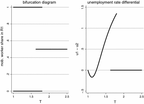
Bifurcation and unemployment
Strictly speaking, there is no unemployment in the periphery when agglomeration is complete since there are no mobile workers present. The unemployment rate in region 2 is defined as the one that would result if a marginal worker decided to leave the core.
Simulation results are omitted.
See Pissarides (1990).
Even if the price for housing does not influence the workers relative fall-back position, it still has an effect on migration decisions, of course.
In our simple model, this just means to hold \(z/W\) constant for all regions. In reality, this might be more complicated because incentives are not only influenced by wages and unemployment benefits.

References
Baldwin RE, Forslid R, Martin P, Ottaviano GIP, Robert-Nicoud F (2003) Economic geography and public policy. Princeton University Press, Princeton
Blanchflower DG, Oswald AJ (1994) The wage curve. The MIT Press, London
Borck R, Pflüger M, Wrede M (2007) A simple theory of industry location and residence choice. IZA Discussion Papers 2862, Institute for the Study of Labor (IZA)
Brakman S, Garretsen H, Gigengack R, van Marrewijk C, Wagenvoort R (1996) Negative feedbacks in the economy and industrial location. J Reg Sci 36:631–652
Brakman S, Garretsen H, Schramm M (2004) The spatial distribution of wages: estimating the Helpman-Hanson model for Germany. J Reg Sci 44(3):437–466
Cahuc P, Zylberberg A (2004) Labor economics. The MIT Press, Cambridge Massachusetts
Dixit AK, Stiglitz JE (1977) Monopolistic competition and optimum product diversity. Am Econ Rev 67(3):297–308
Elhorst JP (2003) The mystery of regional unemployment differentials: theoretical and empirical explanations. J Econ Surv 17(5):709–748
Epifani P, Gancia GA (2005) Trade, migration and regional unemployment. Reg Sci Urban Econ 35(6):625–644
Fingleton B, Fischer M (2010) Neoclassical theory versus new economic geography: competing explanations of cross-regional variation in economic development. Ann Reg Sci 44:467–491
Francis J (2003) The declining costs of international trade and unemployment. J Int Trade Econ Dev 12(4):337–357
Fujita M, Krugman P, Venables AJ (1999) The spatial economy: cities, regions, and international trade. The MIT Press, London
Glaeser EL, Mare DC (2001) Cities and skills. J Labor Econ 19(2):316–342
Gobillon L, Selod H, Zenou Y (2003) Spatial mismatch: from the hypothesis to the theories. IZA Discussion Papers 693, Institute for the Study of Labor (IZA)
Haas A, Möller J (2003) The agglomeration wage differential reconsidered—an investigation using german micro data 1983–1997. In: Broecker J, Dohse D, Soltwedel R (eds) Innovation clusters and interregional competition. Springer, Berlin, pp 182–217
Hanson GH (2005) Market potential, increasing returns and geographic concentration. J Int Econ 67(1):1–24
Harris JR, Todaro MP (1970) Migration, unemployment and development: a two-sector analysis. Am Econ Rev 60(1):126–142
Krugman P (1991) Increasing returns and economic geography. J Polit Econ 99(3):483–499
Matusz SJ (1996) International trade, the division of labor, and unemployment. Int Econ Rev 37(1):71–84
Monfort P, Ottaviano GIP (2002) Spatial mismatch and skill accumulation. CEPR Discussion Papers 3324, C.E.P.R. Discussion Papers
OECD (2006) Employment outlook. Paris
Ortega J (2000) Pareto-improving immigration in an economy with equilibrium unemployment. Econ J 110(460):92–112
Peeters J, Garretsen H (2004) Globalisation, wages and unemployment: an economic geography perspective. In: Brakman S, Heijdra B (eds) The monopolistic competition revolution in retrospect. Cambridge University Press, Cambridge, pp 236–261
Picard PM, Toulemonde E (2001) The impact of labor markets on emergence and persistence of regional asymmetries. IZA Discussion Papers 248, Institute for the Study of Labor (IZA)
Picard PM, Toulemonde E (2006) Firms agglomeration and unions. Eur Econ Rev 50(3):669–694
Pissarides CA (1990) Equilibrium unemployment theory. Basil Blackwell, Oxford
Puga D (1999) The rise and fall of regional inequalities. Eur Econ Rev 43(2):303–334
Redding S, Venables AJ (2004) Economic geography and international inequality. J Int Econ 62(1):53–82
Sasaki M (2007) International migration in an equilibrium matching model. J Int Trade Econ Dev 16(1):1–29
Sato Y (2000) Search theory and the wage curve. Econ Lett 66(1):93–98
Südekum J (2005) Increasing returns and spatial unemployment disparities. Pap Reg Sci 84(2):159–181
Südekum J (2006) Agglomeration and regional costs of living. J Reg Sci 46(3):529–543
Tabuchi T (1998) Urban agglomeration and dispersion: a synthesis of Alonso and Krugman. J Urban Econ 44(3):333–351
Venables AJ (1996) Equilibrium locations of vertically linked industries. Int Econ Rev 37(2):341–359
Ziesemer T (2005) Monopolistic competition and search unemployment. Metroecon 56(3):334–359
Author information
Authors and Affiliations
Corresponding author
Appendix A
Appendix A
1.1 A.1 The firm’s optimization strategy
The current-value Hamiltonian for the firm’s problem is
From the maximum principle it follows that
and
The transversality condition is
The change in the co-state \(\lambda \) (see condition 35) will be zero in steady state. From (5) we know that \(p^{\prime }x/p = -1/\sigma = \rho -1\). Using this and (35) in (36) we get Eq. (17).
1.2 A.2 Wage bargaining
Equation (23) can be rewritten as
or
Using this in a firm-price version of (8) we get
Substituting this version of \(rU\) into (23) and rearranging we get (24). For the partial derivatives of \(g\) we get that \(\partial g/ \partial W > 0\) and \(\partial g/ \partial \theta > 0\) if \(-q^{\prime }(\theta )\theta /q(\theta )<1\), which holds if the matching function is of the Cobb-Douglas type.