
Abstract
In this paper, a fault estimation problem for a class of nonlinear systems subject to multiplicative faults and unknown disturbances is investigated. Multiplicative faults usually mixed with system states and inputs can cause additional complexity in the design of fault estimator due to parameter changes within process. Especially for the nonlinear system corrupted with unknown disturbances, it is not an easy work to distinguish the real fault factor from the mixed term. Under the nonlinear Lipschitz condition, the proposed robust adaptive fault estimation approach not only estimates the multiplicative faults and system states simultaneously, but also extracts the real effect of the faults. Meanwhile, the effect of disturbances is restricted to an L 2 gain performance criteria which can be formulated into the basic feasibility problem of a linear matrix inequality (LMI). In order to reduce the conservatism of the proposed method, a relaxing Lipschitz matrix is introduced. Finally, an illustrative example is applied to verify the efficiency of the proposed robust adaptive estimation scheme.
1 Introduction
Issues and concerns about the system or process safety and reliability necessitate and foster the development of fault detection and diagnosis for dynamical systems, which has been regarded as one of the most important aspects in seeking effective solution to guarantee reliable operation of practical control systems at the possible occurrence of system failures or malfunctions. During the past two decades, significant research results in the area of fault detection and accommodation can be found in some excellent books [1, 3, 4] and survey papers [10, 21].
In order to avoid performance deterioration or system damage, faults have to be found as soon as possible and schemes have to be made to stop propagation of bad effects. Traditional approaches for fault detection and identification are mainly focused on linear systems, which are widely described and well documented in many research articles [5, 7]. However, the majority practical control system are nonlinear in nature. Therefore, nonlinear properties cannot be neglected for the purpose of fault diagnosis and identification. Due to this reason, an active research about nonlinear system fault detection and identification have been brought more and more attention [2, 15, 19].
As one of the most important tasks in a fault detection and identification scheme, fault estimation is for determining the extent of the faults, such as magnitude or frequency of the faults. Accurate fault estimation can help reconstruct the fault signals so that their effects can be accommodated in the corresponding control reconfiguration. Nevertheless, it is not an easy task, especially for the nonlinear system with unknown disturbance. In [13], the authors transformed a nonlinear system with uncertainties into two subsystems under some geometric conditions, and then established an adaptive observer to obtain the estimations of both states and actuator/sensor faults. Yan and Edwards [20] utilized sliding mode observer to realize fault reconstruction. Gao and Ding [8] developed a fault estimator based on a descriptor system formulation for the sensor fault estimation problem. It can simultaneously estimate the states and the sensor fault signal superimposed on the output. Hou [9] provided an effective method to estimate amplitude and frequency of a sinusoidal signal. There are some other methods utilized to tackle fault estimation problems; see, for instance, [18].
As we known, faults can be classified into additive and multiplicative faults according to their effects on the system outputs and the system dynamics. Although component faults and some of actuator/sensor faults appear in the form of multiplicative fault that correspond to parameter changes in the system model, most of the literature about fault estimation paid attention to the effects of additive faults that result in changes only in the mean value of the system output signal. On the other hand, some studies about multiplicative fault estimation are scattered over some papers [6, 10, 17] and book chapters [4, 11]. As the name suggests, it is relatively harder to separate the effects of the faults from the input and states because they are mixed together in a multiplicative form. Therefore, the analysis and design for multiplicative fault estimation is not as straightforward as that for additive faults. Though it is more difficult, the estimation of the real effect of multiplicative faults is given more and more attention. In the recent article [22], a good fault detection and isolation scheme was presented for the system appearing an unknown fault function which was restricted to a finite set of fault types, and each type was described by the product of an unknown parameter vector characterizing the time varying magnitude of the fault with a known smooth vector representing the functional structure of the fault.
Taking into account the above mentioned conditions, in this article, we focus on a Lipschitz nonlinear system subject to multiplicative faults and unknown disturbances. The motivation of our work is to establish a robust adaptive fault estimation scheme which is robust with respect to the disturbance and sensitive to the faults, to detect and estimate multiplicative faults, and get the real effect of faults. Based on Lyapunov stability theory and by relaxing a less conservative Lipschitz condition, an estimator is developed to estimate both the system states and real fault factors simultaneously. The effect of unknown disturbances is reduced according to an L 2 gain performance criterion. Compared to most of the existing work on fault estimation, the proposed scheme is simple to compute, easy to implement, and capable of estimating the actual size of the faulty parameters in the model. Furthermore, an illustrative example is adopted in the simulation study to demonstrate the effectiveness of the proposed fault estimation scheme.
In the remainder of this paper, firstly we provide the Lipschitz nonlinear system with multiplicative faults and unknown disturbances in Sect. 2. A robust adaptive observer based fault estimator is presented in Sect. 3, and the proof for the convergence of the estimator is included. In Sect. 4, a one-link manipulator example is chosen to demonstrate the proposed robust adaptive fault estimation algorithm.
2 Problem Statement
In this paper, we focus on a class of nonlinear multi-input–multi-output dynamical systems described by


where x(t)∈ℝn, y(t)∈ℝm, and u(t)∈ℝp are the state vector, the output vector, and the input vector, respectively. d(t) represents the system disturbance and the L 2 norm of the unknown input d(t) is bounded. A, B, and C are the known system matrices of appropriate dimensions. ϕ(x,u,t) is a Lipschitz nonlinear vector function with a Lipschitz constant δ, i.e.,
It should be noted that Eq. (1) is a general form since most nonlinear functions can be expanded at the equilibrium point. For instance, the nonlinear system \(\dot{x}=f ( x,u,t ) \) is differentiated with respect to x and u, and (x e ,u e ) is the equilibrium point. Applying the Taylor expansion, we can get \(A=\frac{\partial f ( x,u,t ) }{\partial x}|_{x=x_{e},u=u_{e}}\), \(B=\frac{\partial f ( x,u,t ) }{\partial u}|_{u=u_{e},x=x_{e}} \), and ϕ(x,u,t) can be assumed to be the remaining term. Further, many nonlinear functions can be assumed as Lipschitz, at least locally. For example, the sinusoidal function sin(x) appearing in many robotic control systems is globally Lipschitz. And the term x 2 can be regarded as locally Lipschitz within a finite range of x.
Multiplicative Fault Model
With the assumption that the nonlinear system (1)–(2) is subject to component faults which are parameter changes within the process, the post-fault system is modeled as


where θ i (t)∈ℝ, i=1,…,l, are unknown time functions which are assumed to be zero before the fault occurrence, and non-zero after the fault occurrence. g i (x,u,t), i=1,…,l, are known functions related to system states and inputs, which also satisfy Lipschitz condition with a Lipschitz constant δ i . For simplicity, the time t is dropped from the notation in the following equations.
Assumption 1
The multiplicative fault factors θ i , i=1,…,l, are unknown and bounded by a constant, i.e., ∥θ i ∥≤α i , The constant α i is known.
In Eq. (4), the term \(\sum_{i=1}^{l}\theta_{i} ( t ) g_{i} ( x,u,t ) \) is generated by the multiplicative faults. This representation characterizes a general class of multiplicative faults where θ i represents the magnitude of the time-varying or constant fault and g i characterizes the functional structure of the ith fault. Multiplicative faults encountered in a linear system were modeled in the excellent book [4], which can be transformed into this kind of representation. For example, the linear system \(\dot{x}= ( A+A_{f} ) x\) is subject to multiplicative faults in the form \(A_{f}=\sum_{i=1}^{l}A_{i}\theta_{A_{i}}\), so we can get the structure function g i =A i x. In practice, component faults in the process and some of faults in the sensors and actuators are in the form of multiplicative faults, which changes system parameters and usually mixes with system states and inputs. Hence such faults result in performance degradation or even instability of the system. Let \(f=\sum_{i=1}^{l}\theta_{i} ( t ) g_{i} ( x,u,t ) \), we can rewrite Eq. (4) as
It is clear that f is a term induced by the component faults θ i , i=1,…,l. When the system is in normal operation, f=0. The form in Eq. (6) has been adopted to treat the additive fault estimation, where the size of f can be estimated. However, it is clear that in modeling the system component faults, the term f is also a function of the system state and input. f alone cannot reflect the real fault sources or size. Therefore, it is necessary for us to estimate the real fault factors θ i , i=1,…,l, instead of the additive fault vector f.
Relaxing Lipschitz Condition
The Lipschitz condition (3) can be given in a relaxing matrix form which is defined as
The matrix H could be a sparsely populated matrix. There is an example to illustrate that \(\Vert H ( x ( t ) -\hat{x} ( t ) ) \Vert _{2}\) is much smaller than \(\delta \Vert x ( t ) -\hat{x} ( t ) \Vert _{2}\) for the same nonlinear function in [16]. The relaxing Lipschitz condition (7) is much less conservative.
Design Objective
The objective of this paper work is to design an adaptive estimator with an effective algorithm for nonlinear system (1)–(2) subject to multiplicative faults to estimate the real effect factor θ i , i=1,…,l, in the post-fault system (4)–(5), and make the estimation accurate and insensitive to the unknown disturbances.
In order to design an estimator satisfying the above objective, it is assumed that the system states and inputs are all bounded before and after the occurrence of a fault, and the Lipschitz nonlinear functions ϕ(x,u,t) and g i (x,u,t) satisfy the relaxing Lipschitz condition with matrices H and G i . It should be noted that the feedback control system is capable of making the system bounded even in the presence of a fault. The proposed fault estimation design is independent on the structure of the feedback controller.
3 Robust Adaptive Fault Estimation
In this section, an adaptive observer is applied to reconstruct multiplicative fault signals which are mixed with system states and inputs. The designed adaptive observer here for the nonlinear system (1)–(2) can be shown to be as follows:


where σ i >0, i=1,…,l are constants, \(\hat{x}\), \(\hat{y,}\) and \(\hat{\theta}_{i}\) denote the estimated state, output, and fault variables, respectively. L and D are the design gain matrices. Let \(e_{x}=x-\hat{x}\) and \(e_{y}=y-\hat{y}\) represent the state and output estimation error; \(e_{\theta _{i}}=\theta_{i}-\hat{\theta}_{i}\) denotes fault error. Then we obtain the following estimation error dynamic equations


The main problem encountered here is that the system is subject to unknown disturbance and the real fault effect factor θ i which is combined with the system state x and input u. We must design an appropriate estimator which can estimate the fault θ i effectively and be less sensitive to the disturbance.
At first, let us introduce a lemma and a definition which are useful for the analysis of this multiplicative fault estimation problem.
Lemma 1
(Barbălat’s Lemma [12])
If \(\lim_{t\rightarrow \infty }\int_{0}^{t}f ( \tau ) \,d\tau \) exists and is finite, and f(t) is a uniformly continuous function, then lim t→∞ f(τ)=0.
Definition 1
(Persistence of Excitation [12])
A piecewise continuous signal vector ϕ:ℝ+↦ℝn is called Persistence of Excitation in ℝn with a level of excitation α 0>0 if there exist constants α 1, T 0>0 such that
In the analysis of the estimation error functions (11)–(13), a sufficient condition for asymptotic stability of the observer is presented and proved in the following theorem.
Theorem 1
Suppose the pair (A,C) is observable, and the matrix C is of full row rank. Assume that g i (x,u,t), i=1,…,l, are persistence of excitation. If there is a positive definite matrix P=P T>0 and a matrix D such that


then the observer-based estimator (8)–(10) ensures that
-
1.
The estimated x and \(\hat{\theta}_{i}\) asymptotically converge to the nonlinear system state x and the multiplicative fault θ i respectively under the zero disturbance case.
-
2.
When the unknown disturbance exists, the output error satisfies \(\Vert e_{y}\Vert _{2}^{2}<\gamma^{2}\Vert d\Vert _{2}^{2}\).
Proof
The proof consists of two parts: the internal stability analysis and computing the robust performance index.
-
1.
Internal stability analysis.
Choose \(V ( t ) =e_{x}^{T} ( t ) Pe_{x} ( t ) +\sum_{i=1}^{l}\sigma_{i}^{-1}e_{\theta _{i}}^{T} ( t ) e_{\theta _{i}} ( t ) \) as the Lyapunov function and calculate the derivative of the Lyapunov function V(t). We get

According to Lipschitz condition, we have

Then the derivative of the Lyapunov function satisfies the following inequality:
$$ \dot{V}\leq e_{x}^{T} ( \varLambda ) e_{x}+2e_{x}^{T}Pd. $$(17)In the zero disturbance case, one has
$$ \dot{V}\leq -\lambda_{\min } ( -\varLambda ) \Vert e_{x} \Vert ^{2}. $$(18)Based on Schur Complement Lemma, the matrix Λ is a negative definite matrix. Inequality (18) indicates e x ∈L 2. Because e x ∈L ∞, \(\dot{e}_{x}\) is uniformly bounded. Based on Barbǎlat’s Lemma, we have e x →0 as t→0. And due to persistent excitation condition of g i (x,u), the estimator (8)–(10) ensures that \(e_{\theta _{i}}\rightarrow 0\) as t→0.
-
2.
Robust Performance Index.
Defining
$$ J=\dot{V}+e_{y}^{T}e_{y}-\gamma^{2}d^{T}d $$and using Eq. (17), we can derive that
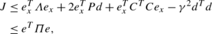
where
$$ e=\left [ \begin{array}{c@{\quad}c} e_{x}^{T} & d^{T}\end{array} \right ]^{T}. $$It follows that
$$ J\leq -\lambda_{\min } ( -\varPi ) \Vert e\Vert ^{2}. $$Under the zero initial condition, we have
$$ \int_{0}^{T} \bigl( e_{y}^{T}e_{y}- \gamma^{2}d^{T}d \bigr) \,dt=\int_{0}^{T}J\,dt-V ( T ) <0, $$which implies
$$ \int_{0}^{T}e_{y}^{T}e_{y}\,dt \leq \gamma^{2}\int_{0}^{T}d^{T}d \, dt $$This completes the proof of the theorem.


□
Remark 1
Based on Schur Complement Lemma, and letting Y=PL, Π<0 in Eq. (14) can be rewritten as the following matrix inequality:

The matrix D can be derived from
Remark 2
A good estimator is designed to make the whole system sensitive to the multiplicative fault and insensitive to the disturbance. Hence, we can reduce the effect of disturbance d to the formula (14) with a smaller γ using Matlab LMI toolbox.
4 An Illustrative Example
In this section, we consider a one-link manipulator with revolute joints actuated by a DC motor, which is an excellent example used to verify design schemes in many works [14, 16, 22]. The corresponding state-space model with no faults and disturbance is

where q 1 and q m are the angular position of the link and motor, respectively, ω 1 is the angular velocity of the link, and ω m is the angular velocity of the motor. J 1 and J m are the inertia of the link and motor. The control u is the torque of the motor. The nonlinear system with multiplicative fault and disturbance is shown in the following:

with
The unknown disturbance is d=[0 d 1 0 d 2]T, where the L 2 norms of d 1 and d 2 are assumed to be bounded. Two types of component faults are considered here.
Case 1: An abnormal friction appears in the motor which leads to parameter changes in the system state matrix. Suppose that the viscous friction constant B increases by 20 % at t=5 seconds. In this case, θ 1∈[0,1] represents the real multiplicative fault parameter. When θ 1=0, the system is in the normal operation. θ 1=0.2 at t=5 seconds. And the viscous friction fault structure function g 1=[0 −1.25x 2 0 0]T.
Case 2: The actuator occurs multiplicative fault which is in the form of \(u= ( 1+\theta_{2} ) \bar{u}\). θ 2∈[−1,0] represents the magnitude of the fault. When θ 2=0, the actuator is in the normal operation, while θ 2=−1 represents the complete fault of the actuator. And the fault structure function is g 2=[0 21.6u 0 0]T. Here we suppose that the actuator efficiency decreases by 30 % at t=15 seconds.
The nonlinear term ϕ is a Lipschitz nonlinear function with a global Lipschitz constant δ=3.33. And the relaxing Lipschitz matrix is
Based on multiplicative fault estimation strategy we proposed in Sect. 3, the robust adaptive multiplicative fault estimator is established. The simulation of the robust adaptive fault estimation is performed in Simulink. A sinusoidal wave input of this system is given by u=sin(t). The initial condition is x(0)=0. According to Theorem 1, the observer gain is obtained with a robust performance γ 2=0.3 shown here
Figure 1 shows the output estimation error for the system subject to an extra abnormal friction fault. Figure 2 illustrates the estimated multiplicative fault θ 1. The fault is accurately estimated compared to the desired trajectory. Figures 3 and 4 depict the output estimation error and the estimation of multiplicative fault θ 2 when the actuator efficiency degradation occurs in the system. Again the fault is successfully estimated. From these simulation results, we can see that the proposed robust adaptive estimation scheme not only guarantees the state estimation and multiplicative fault estimation accurately, but also makes the estimator insensitive to the unknown disturbances.

Output estimation error under the abnormal friction fault

The estimation of viscous friction

Output estimation error under actuator fault

The estimation of actuator fault
5 Conclusion
In this paper, a robust adaptive fault estimation scheme has been proposed for a kind of Lipschitz nonlinear system subject to multiplicative faults and unknown disturbances. Multiplicative faults are parameter changes within the process which make the design for fault estimation more complicated. The estimator is designed in the context of a trade-off between robustness to disturbances and sensitivity to faults. According to Lyapunov stability theory, the estimator can estimate the real fault factors accurately, and simultaneously estimate the system states. The conservatism for the whole fault estimation scheme is reduced by using a relaxing Lipschitz matrix. The proposed adaptive fault estimation algorithms have been verified by a one-link manipulator control system.
References
M. Blanke, M. Kinnaert, J. Lunze, M. Staroswiecki, Fault Diagnosis and Fault-Tolerant Control, 2nd edn. (Springer, Berlin, 2006)
J.D. Boskovic, S.E. Bergstrom, R.K. Mehra, Robust integrated flight control design under failures, damage, and state-dependent disturbances. J. Guid. Control Dyn. 28(5), 902–917 (2005)
J. Chen, R.J. Patton, Robust Model-Based Fault Diagnosis for Dynamic Systems. (Kluwer Academic, Norwell, 1999)
S.X. Ding, Model-Based Fault Diagnosis Techniques: Design Schemes, Algorithms, and Tools (Springer, Berlin, 2008)
G.R. Duan, R.J. Patton, Robust fault detection using Luenberger-type unknown input observers—a parametric approach. Int. J. Syst. Sci. 32(4), 533–540 (2001)
S.X. Ding, P.M. Frank, E.L. Ding, An approach to the detection of multiplicative faults in uncertain dynamic systems, in Proceedings of the 41st IEEE Conference on Decision and Control (2003), pp. 4371–4376
P.M. Frank, Fault diagnosis in dynamic systems using analytical and knowledge-based redundancy—a survey and some new results. Automatica 26(3), 459–474 (1990)
Z. Gao, S.X. Ding, Actuator fault robust estimation and fault-tolerant control for a class of nonlinear descriptor systems. Automatica 43(5), 912–920 (2007)
M. Hou, Estimation of sinusoidal frequencies and amplitudes using adaptive identifier and observer. IEEE Trans. Autom. Control 52(3), 493–499 (2007)
R. Isermann, Model-based fault-detection and diagnosis-status and applications. Annu. Rev. Control 29(1), 71–85 (2005)
R. Isermann, Fault-Diagnosis Systems (Springer, Berlin, 2006)
P.A. Ioannou, J. Sun, Robust Adaptive Control (Prentice Hall, Englewood Cliffs, 1996)
B. Jiang, M. Staroswiecki, V. Cocquempot, Fault diagnosis based on adaptive observer for a class of non-linear systems with unknown parameters. Int. J. Control 77(4), 367–383 (2004)
B. Jiang, M. Staroswiecki, V. Cocquempot, Fault accommodation for nonlinear dynamic systems. IEEE Trans. Autom. Control 51(9), 1578–1583 (2006)
C.D. Persis, A. Isidori, A geometric approach to nonlinear fault detection and isolation. IEEE Trans. Autom. Control 46(6), 853–865 (2001)
G. Phanomchoeng, R. Rajamani, Observer design for Lipschitz nonlinear systems using Riccati equations, in American Control Conference (2010), pp. 6060–6065
C.P. Tan, C. Edwards, Multiplicative fault reconstruction using sliding mode observers, in 5th Asian Control Conference (2004), pp. 957–962
K. Vijayaraghavan, R. Rajamani, J. Bokor, Quantitative fault estimation for a class of non-linear systems. Int. J. Control 80(1), 64–74 (2007)
A. Xu, Q. Zhang, Nonlinear system fault diagnosis based on adaptive estimation. Automatica 40(7), 1181–1193 (1994)
X.G. Yan, C. Edwards, Nonlinear robust fault reconstruction and estimation using a sliding mode observer. Automatica 43(9), 1605–1614 (2007)
Y. Zhang, J. Jiang, Bibliographical review on reconfigurable fault-tolerant control systems. Annu. Rev. Control 32(2), 229–252 (2008)
X. Zhang, M.M. Polycarpou, T. Parisini, Fault diagnosis of a class of nonlinear uncertain systems with Lipschitz nonlinearities using adaptive estimation. Automatica 46(2), 290–299 (2010)
Author information
Authors and Affiliations
Corresponding author
Rights and permissions
About this article
Cite this article
Gao, C., Duan, G. Robust Adaptive Fault Estimation for a Class of Nonlinear Systems Subject to Multiplicative Faults. Circuits Syst Signal Process 31, 2035–2046 (2012). https://doi.org/10.1007/s00034-012-9434-x
Received:
Revised:
Published:
Issue Date:
DOI: https://doi.org/10.1007/s00034-012-9434-x