
Abstract
The time span of surface thermal data bases now reaches a few decades. However, studies using surface thermal time series are seldom, due to the difficulty of obtaining temporally coherent estimations for this parameter. Applications for surface thermal multitemporal analysis range from climate change studies and modeling to anomaly detection for natural or industrial hazard detection. This chapter presents methods to improve the temporal coherence of temperature time series, through data reconstruction of atmospheric and cloud contaminated observations, and through the correction of the orbital drift effect which hinders the use of the longest data sets. Then, methods for the analysis of time series are presented, including both image to image comparison and trend detection, the choice between these methods depending on the spatial resolution of the dataset and the aims of the considered study.
Access provided by Autonomous University of Puebla. Download chapter PDF
Keywords
- Time Series
- Land Surface Temperature
- Atmospheric Correction
- Enhance Vegetation Index
- Bidirectional Reflectance Distribution Function
These keywords were added by machine and not by the authors. This process is experimental and the keywords may be updated as the learning algorithm improves.
14.1 Introduction
Although thermal remote sensing data have been available since the 1970s, the use of time series in remote sensing is recent, since the temporal coherence of thermal data records have been hindered by several flaws. Nonetheless, the potential of the applications is high, from climate change studies to environment monitoring.
As concern about the consequences of climate change grows, the need for reliable information on surface temperature has increased. For example, climate modelers need surface temperature as input for their models to adequately simulate past and future climate, in order to be able to quantify vegetation and plankton response to atmospheric CO2 anthropogenic forcing (see for example Diak and Whipple 1993). As stated by Frey et al. (2012), “surface temperature is a key variable in the climatological system. It represents the interface between the incoming radiation fluxes and other terms of the energy balance, i.e. the sensible heat flux or the ground heat flux. Air temperature is directly triggered by Land Surface Temperature (LST). Because of this central position in the climatological system, LST can be used as an indicator of the energy balance at the Earth’s surface and the so-called greenhouse effect in climate change studies. As part of the surface radiation budget, LST belongs also to the essential climate variables of WMO-GCOS (World Meteorological Organization-Global Climate Observing System, URL1). In the Strategic Plan for the US Climate Change Science Program (CCSP 2006), the surface ground temperature is listed as a state variable and the long-wave surface energy budget (derived also from LST) is listed as one of its key external forcing or feedback observations” (Frey et al. 2012).
This need for reliable surface thermal estimations is also shared by studies on climate change’s current consequences. For example, it allows the identification of desertification (Lambin and Ehrlich 1996; Karnieli et al. 2010), whether under water stress or human pressure. Surface temperature is also a key parameter for ecosystem studies, since the suitability of temperature conditions for local flora and fauna species is endangered by climate change (see for example Bertrand et al. 2011).
Thermal estimations include both temperature and emissivity, which are intimately related (see for example Gillespie et al. 1998, for temperature and emissivity separation methods). Thermal emissivities have been monitored for their inclusion in global climate model surface schemes (Menglin and Liang 2006), and their seasonal variation analyzed (Ogawa et al. 2008). Thermal emissivities can also be used to monitor vegetation changes through time, as French et al. (2008) have presented for a semi-arid site in New Mexico (USA).
Another field of application of thermal remote sensing is thermal anomaly detection and monitoring. These approaches are carried out by comparing pixel temperatures against their background in uni-temporal satellite data (Kuenzer et al. 2007), or they consist in comparing a near-real time surface temperature estimation to past reference measurements, in order to identify departures from standard behaviors (Kuenzer et al. 2008). Some modern fire detection systems have been developed based on this principle, and are especially useful for detection of fire events in remote areas (Prins et al. 2004). Such alert systems can also be implemented for volcano monitoring, or for industrial hazard detection.
However, for such applications to be implemented, one key aspect has to be taken into account: when two thermal images are compared at two distinct dates, one has to make sure that both images are coherent. Some of the factors that decreases the temporal coherence in multitemporal thermal analysis are common to other remote sensing characterization, while others are more TIR (Thermal Infra Red) specific. All these factors are summarized in Table 14.1.
Common factors with other remote sensing applications are included in what is generally referred to as level 2 products, which include calibration, georeferencing, and atmospheric correction. Calibration is needed to transform sensor counts into brightness temperature, is sensor dependent, and calibration coefficients may need to be updated during the activity period of a given sensor. Georeferencing is crucial for time series analyses, in order to make sure that the same location is being monitored through time. Regarding atmospheric correction, some land and sea surface temperature algorithms (Jiménez-Muñoz and Sobrino 2008; Barton 1995) consider the absorption due to total atmospheric water content, while others only transform brightness temperatures to land surface temperature through the assignation of land surface emissivities (Sobrino et al. 2008a). Additionally, complex atmospheric correction may be needed, especially considering the impact of atmospheric depth, atmospheric mass, and also terrain on the thermal signal, such as provided by the ATCOR (atmospheric correction) tool, implemented for thermal bands of Landsat MSS (Multispectral Scanner), TM (Thematic Mapper) or ETM+ (Enhanced Thematic Mapper Plus), ASTER (Advanced Spaceborne Thermal Emission and Reflection Radiometer ) or BIRD (Bispectral Infra-Red Detection) instruments, and available in various software packages.
However, time series pre-processing of thermal remote sensing data also present more specific characteristics. The first one, which is shared with other optical remote sensing, is the presence of clouds, which mask the land surface and therefore prevent from the estimation of surface temperature. Additionally, in high resolution data, projected cloud shadows can also decrease the retrieved temperatures. Cloud masks are sometimes provided with temperature retrievals, although undetected clouds may still be present in the data. For example, thin cirrus clouds decrease the observed surface temperature, although their detection from remotely sensed data is problematic (Saunders and Kriebel 1988). Moreover, some regions of the globe are almost permanently covered with clouds during some seasons, and therefore cloud free observations are scarce, and time series gap filling has to be implemented.
Another specific aspect of time series analysis in thermal remote sensing is the orbital drift effect. This orbital drift effects all satellites which do not possess onboard fuel for orbit correction, such as engineless platforms, or ageing platforms which fuel reserves have been exhausted. Orbital drift is evidenced mainly for polar satellites, and consists in a slow but steady change in the orbit characteristics of the considered satellite, which results in an increasing delay or advance in satellite overpass over a given reference geographic location. An example of such orbital drift can be observed in the case of the NOAA (National Oceanic and Atmospheric Administration) satellite series (Price 1991). The effect of the orbital drift combines both considerations on sun-target-sensor geometry (proportion of shade in a given pixel) as well as on daily temperature cycle characteristics, to which the resulting variations in the pathway length through the atmosphere can be added. Therefore, it is evidenced more easily for land covers with high daily amplitude (deserts, crops) than for low amplitudes (sea, evergreen forests). A similar effect can be evidenced for non-drifting platforms for which some pixels are observed for different paths. However, this effect is not correlated with time, and therefore can be assimilated as an additional noise in the time series which can be handled by the trend detection methods presented in Sect. 14.3.2.
Thermal anisotropy is another factor which can influence temperature retrieval, and therefore thermal time series (Lagouarde et al. 1995), for which a BRDF-type (Bidirectional Reflectance Distribution Function, see Tanré et al. 1983) correction could be developed. However, since such correction has not yet been developed in the case of thermal data, it will not be mentioned further here.
In order to be able to analyze thermal time series (whether emissivities or temperatures) correctly, all these aspects have to be taken into consideration. Then, change analysis can be conducted. To that end, this chapter is divided into two parts, the first part describing how to conduct these corrections, while the second one is focused specifically on change analysis.
14.2 Removal of Temporal Incoherence in Thermal Time Series
As stated in the introduction, the coherence of thermal time series can be hindered by several factors. Since factors such as calibration, geocorrection, and atmospheric correction are usually taken into account during data processing, they will not be elaborated on here. Instead, this first part will be devoted to the correction of two more specific factors, i.e. cloud contamination and orbital drift effects.
14.2.1 Cloud Contamination
The first step in cloud contamination removal is cloud identification. It is usually carried out through band ratio and/or band thresholding, with each band or band ratio threshold aiming at the detection of one particular type of cloud (high and low thick clouds, thin cirrus) for both Land Surface Temperature and Sea Surface Temperature (SST). The key point here is the number of bands available for the considered sensor, which allow for more or less thresholds to be applied. When restricted to thermal infrared, the application of thresholds is less reliable, especially when the observed areas may present an ice or snow cover during part of the time series (mountains, temperate to polar areas). This is due to the fact that cloud tops have similar temperatures to snow or ice covered surfaces. Recent algorithms allow for a good assessment of cloud contamination (Ackerman et al. 1998; Derrien and Le Gléau 2005). Nevertheless, cloud masking may leave out cloud contaminated values in the time series, which is the reason why this section will focus on cloud reconstruction methods.
Cloud reconstruction methods are based on a few assumptions, which allow identifying cloud contaminated values within the temporal profile of the data, and then filling the gap corresponding to cloud contaminated values. Usually, the assumptions made for reconstruction are threefold (Julien and Sobrino 2010): continuity of the time series, which corresponds to the fact that observed natural processes show slow changes; clouds have an unidirectional effect on the signal, which is due to the fact that usually cloud contamination tend to decrease the signal values; and finally, cloud free dates are sufficient for time series reconstruction. Most methods for time series reconstruction have been developed for analyses of vegetation index time series (such as NDVI – Normalized Difference Vegetation Index, Tucker 1979, or EVI – Enhanced Vegetation Index, Huete et al. 2002). However, these methods can also be applied to sea or land surface temperature as well as to emissivity time series. Such methods are reviewed in the following paragraphs, to focus finally on three methods selected for their wide application or their novelty.
Numerous methods have been presented to identify and interpolate contaminated values in time series data (van Dijk et al. 1987; Viovy et al. 1992; Roerink et al. 2000; Jönsson and Eklundh 2002, 2004; Chen et al. 2004; Ma and Veroustraete 2006; Beck et al. 2006; Julien and Sobrino 2010), the latest methods usually performing better than the previous ones (Hird and McDermid 2009). The criteria usually followed to assess the best reconstruction method are its fidelity to the original cloud-free data and its ability to identify cloud contaminated values. Validation of the reconstructed time series is usually qualitative, since spatially extensive measurements (usually of the order of one square kilometer) would be needed for a quantitative validation. Readers have to keep in mind that such corrections reconstruct a “clear-sky” time series, which can differ substantially from ground truth, since cloudy LST for example would be lower than the reconstructed “clear-sky” value. However, estimation of cloudy LST would require the inclusion of models that would increase considerably the processing costs of the correction, which is the reason why such methods have not been developed widely. One example of such method can be found in Jin and Dickinson (2000). Note that these methods do not distinguish between clouds and other atmospheric contamination of the data.
The methods presented by van Dijk et al. (1987) and Viovy et al. (1992) were designed with their application to daily time series in mind, and therefore are difficult to apply on composited time series, due to their focus on the highest frequencies in the signal (up to a few days), which do not appear in composited time series. Indeed, most of the publicly available databases of remotely sensed data for Earth observation, such as Pathfinder AVHRR (Advanced Very High Resolution Radiometer) Land (Smith et al. 1997) or GIMMS (Global Inventory Modeling and Mapping Studies; Tucker et al. 2005) are composited. This compositing aims at lowering atmospheric and cloud influence, as shown in Holben (1986), with different compositing periods ranging usually from 8 to 15 days. Even though composite data present lower atmospheric contamination than raw time series, this composition process does not eliminate atmospheric contamination. For example, cloud cover can persist longer than the compositing period for some time periods (rainy season) or over some specific areas (tropical rainforests). Therefore, we present here three approaches for remaining atmospheric influences on composited time series:
HANTS (Harmonic Analysis of NDVI Time Series): This algorithm (Menenti et al. 1993; Verhoef et al. 1996; Roerink et al. 2000) was developed with the application to time series of NDVI images in mind. These images are usually composited by means of the so-called Maximum Value Compositing (MVC, Holben 1986) algorithm in order to suppress atmospheric effects. The HANTS algorithm exploits the negative effect of atmospheric contamination on NDVI values. In HANTS, a curve fitting is applied iteratively, i.e. first a least squares curve is computed based on all data points, and next the observations are compared to the curve. Observations that are clearly below the curve are candidates for rejection due to atmospheric contamination and the points that have the greatest negative deviation from the curve therefore are removed first. Next a new curve is computed based on the remaining points and the process is repeated. Pronounced negative outliers are removed by assigning a weight of zero to them, and a new curve is computed. This iteration eventually leads to a smooth curve that approaches the upper envelope of the data points. In this way, atmospheric contaminated observations have been removed and the amplitudes and phases computed are much more reliable than those based on a straightforward FFT (Fast Fourier Transform). An example of implementation of the HANTS algorithm for land surface temperature time series analysis can be found in Julien et al. (2006).
Double logistic curve fitting: The double logistic approach has been previously applied in Julien and Sobrino (2009) to global GIMMS data, as a generalization of the method presented by Beck et al. (2006) for Siberia.
NDVI yearly evolutions are fitted to the following double logistic function (Beck et al. 2006):
where NDVI(t) is the remotely sensed NDVI evolution for a given year (t = 0 to 364, in day of year), wNDVI is the winter NDVI value, mNDVI is the maximum NDVI value, S is the increasing inflection point (spring date), A is the decreasing inflection point (autumn date), mS is related to the rate of increase at S inflection point, and mA is related to the rate of decrease at A inflection point. All these parameters are retrieved iteratively on a pixel-by-pixel basis, by using the Levenberg-Marquardt technique (More 1977). In order to remove eventual snow- or cloud-contaminated values, a preliminary fit is conducted in order to estimate the dormancy period as the period before spring date and after autumn date. During this period, all eventual negative NDVI values are set to the highest positive value over the whole dormancy period, labeled winter NDVI. Since surface temperatures usually present a high seasonality, this approach is also suitable for surface temperature time series. Although NDVI and LST annual curves may differ in shape (no constant LST during winter or summer), the double logistic approach can describe adequately the LST annual curves.
IDR (iterative Interpolation for Data Reconstruction): This method (Julien and Sobrino 2010), also exploits the tendency of cloud and atmospheric influence to lower NDVI values. Additionally, since NDVI is a proxy for vegetation greenness, its temporal variation should be smooth and continuous. Therefore, for each date of a given time series, an alternative NDVI value is computed as the mean between the immediately preceding and following observations. An alternative NDVI time series is therefore obtained, and compared to the original time series. The date corresponding to the maximum difference between the alternative and original time series is identified, and the corresponding NDVI value in the original time series is replaced with the corresponding NDVI value in the alternative time series. This replacement is carried out only when the maximum difference between both time series is higher than noise level (in that case 0.02 NDVI units). Then a new alternative time series is computed from the modified time series, and the process is iterated until convergence is reached. This process allows to progressively increase one by one the low and discontinuous NDVI values (corresponding to atmospherically contaminated values) until the upper envelope of the NDVI time series is reached. The methodology is somewhat similar to the one presented in Ma and Veroustraete (2006), with the difference that the IDR method is carried out from the data itself, and not from a comparison to an average of different years, which can be problematic for areas with high interannual variability, for areas suffering a land cover change, or when the acquired time series length is short.
Figure 14.1 presents an example of atmospheric contamination reconstruction using the IDR method with Meteosat Second Generation land surface temperature data, retrieved during one whole day by using the algorithm developed by Sobrino and Romaguera (2004). Cloud contamination appears as sudden decreases in retrieved land surface temperature from 10:00 to 13:00 (GMT), while atmospheric contamination is more easily evidenced at night (from 17:00 to 24:00 GMT for example).

One-day (15th July 2010) land surface temperature (in Kelvin) for a pixel in eastern Turkey as retrieved by Meteosat Second Generation SEVIRI (Spinning Enhanced Visible and InfraRed Imager) sensor (black), and after IDR atmospheric contamination reconstruction (grey). See text for details on the IDR method
14.2.2 Orbital Drift Effect
The orbital drift effect is evidenced only for a few platforms, although these platforms are the ones that provide one of the longest time series of surface temperature. Therefore, the following paragraph describes only methods developed to counterbalance this phenomenon for the NOAA-AVHRR sensor.
The first method, developed by Gutman (1999), relies on the previous calculations of temperature and SZA (Solar Zenithal Angle) time series anomalies, which are then averaged over homogeneous vegetation classes. A simple linear regression is then conducted between these averaged anomalies, and finally, the fitted SZA anomalies are removed from LST time series by simple difference. This method was applied and analyzed thoroughly in Gleason et al. (2002), showing that some hemispherical and local adaptations were needed for desert and crop classes respectively. These methods rely on a priori knowledge on land cover, which can (and should) not be considered in change studies through time series analysis.
Another method, developed by Jin and Treadon (2003), relies on modeling land surface temperature daily cycle, from which the difference of temperature between the nominal and actual satellite overpass times can be estimated, and then added to the data for the corresponding date. However, the daily cycles have been computed for 18 land covers, for all four seasons, and for latitude bands of 5°, which transforms temporal discontinuities in land surface temperatures at satellite transitions into spatial discontinuities at vegetation class and latitude band transitions.
Pinheiro et al. (2004) developed a model based on vegetation structural data and geometric optics, which allows for the estimation of the fraction of sunlit and shaded endmembers observed by AVHRR for each pixel of each overpass. This approach has been used to build a daily record of NOAA-14 AVHRR land surface temperature over Africa (Pinheiro et al. 2006). Due to the needed a priori knowledge of the land cover and to the model complexity this approach is difficult to implement for large datasets.
Pinzon et al. (2005) used an approach based on the Empirical Mode Decomposition (EMD) to correct NDVI data for the orbital drift. The decomposition uses the simple assumption that any data consists of different simple intrinsic modes of oscillations, which can be retrieved iteratively from the data itself. Therefore, a specific mode could be identified as orbital drift dependent, and removed from the signal. This approach was chosen for the correction of GIMMS NDVI as well as for the LTDR (Long Term Data Record) dataset.
Finally, Sobrino et al. (2008b) presented a simple and automated method to correct NOAA-AVHRR orbital drift, also using SZA anomaly information. The iterative character of this method results in increased processing times, and is thus difficult to implement for large databases.
All the methods presented above are unable to correct the orbital drift effect without introducing spurious trends in the data (Hou and Shi 2011), since the differentiation between orbital drift and trends included in the time series is not always obvious. However, Julien and Sobrino (2012) developed a data-driven method to correct this orbital drift, therefore avoiding the lack of information on NOAA-AVHRR acquisition times (although indirect approaches such as the ones presented in Frey et al. 2012, or Ignatov et al. 2004, allow for their estimation). The Julien and Sobrino (2012) approach is based on a pixel-by-pixel fit of LST anomalies against both time since launch and solar zenithal angle anomaly, which allows for the removal of orbital drift influence without removing eventual trends in the pixel time series. Figure 14.2 presents an example of the orbital drift influence on a barren pixel time series and its correction by the Julien and Sobrino (2012) approach.

LST time series for a barren pixel before (grey) and after (black) the Julien and Sobrino (2012) orbital drift correction. The orbital drift effect on the uncorrected LST time series is clearly evidenced by the increasing difference between both curves from satellite launch to retirement dates
14.3 Time Series Analyses
In the case of sea surface temperatures, the main application being climate modeling, basic approaches relying on anomaly estimation and linear regression have been generally applied (see for example Comiso 2003). Another case of time series analyses based on anomaly estimation is the coal fire detection method presented by Kuenzer et al. (2008), which also presents the particularity of using four observations per day, as a rare example of intra-daily time series application. Due to the scarcity of temporally coherent land surface temperature time series, few methods have been developed specifically for their analysis. However, methods developed for other optical wavelengths can easily be transposed to thermal infrared applications. Therefore, the following methods could also perfectly be applied to LST time series as well. These methods are presented hereafter, divided in change detection and trend retrieval methods.
14.3.1 Change Detection
Coppin et al. (2004) have reviewed different methods for vegetation monitoring. This section summarizes the ones that are relevant to thermal time series, completed with other references. Detection of changes in remotely sensed images presupposes having access to similar data, whether regarding acquisition (cloud free images, atmospheric effects, illumination and observation geometry, similar wavelengths and spatial resolutions), time scale (comparable phenological state of the vegetation), data processing (similar methods, accurate georeferenciation). Change detection algorithms are mainly based on bi-temporal analysis, i.e. comparison of two sets of data, preferably from before and after the change.
-
A first technique for change detection is univariate image differencing, which consists in the simple subtraction of two images previously co-georeferenced (Banner and Lynham 1981; Lyon et al. 1998; Nelson 1983). Negative differences can generally be attributed to increase in vegetation cover (which temperature is lowered by increased evapotranspiration), while positive differences evidence mainly a decrease in vegetation cover. An example of this method can be found in Fig. 14.3, where the difference between two land surface temperature estimates from airborne AHS (Airborne Hyperspectral Scanner) sensor, acquired over an agricultural area in southern France in 2007 at 11:40 UTC, shows the land cover change between two dates. This difference image allows the identification of the changes suffered between these two dates: lower river (Garonne) level (top of the image, in white), increase in vegetation cover (as a decrease of LST in the lower part of the image, in dark grey) and decrease in vegetation cover (as an increase in LST in the left part of the image, in white). This method has the advantage of low cost in processing time.
Fig. 14.3 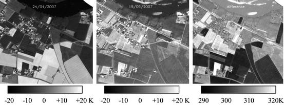
Land surface temperature as retrieved by the AHS (Airborne Hyperspectral Scanner) sensor over an agricultural area in Southern France on 24th April 2007 and 15th September 2007 (upper images) and their difference (lower image)
-
A second technique consists in image ratioing on a pixel by pixel basis, resulting in an image where change pixels have a value different to unity. This technique has been applied by Howarth and Wickware (1981), unfortunately without being able to make a quantitative assessment of the changes.
-
A third technique is image regression, which consists in assuming that the “after” image is linearly related to the “before” image for all bands, implying that the spectral properties of most pixels have not changed between images. Changes are then identified by setting thresholds to the residuals. This technique has not been proven to reach high accuracies (Burns and Joyce 1981; Singh 1989; Ridd and Liu 1998).
-
A fourth method is multi-temporal spectral mixture analysis, which supposes that the images (preferably with high spatial resolution) include pixels with pure spectral signatures or end-members, present in all pixels with different proportions. Then, change results in variation in end-member percentiles. This method was implemented successfully for Landsat images of Brazilian Amazon by Adams et al. (1995) and Roberts et al. (1998).
-
Finally, a fifth technique is multidimensional temporal feature space analysis, which consists in overlaying selected bands of the “before” and “after” images in a composite image as red, green and blue bands, in which changes appear in unique colors. This technique does not provide any insight on the drivers of the changes, and is usually applied for mask building before change detection. For example, Alwashe and Bokhari (1993) and Wilson and Sader (2002) have applied this technique to Landsat bands or derived indices. Finally, combinations of those different techniques have also been used (Desclée et al. 2006).

Among all these techniques, users should choose which method is more adequate for their application. For example, methods 1, 2 and 5 are straightforward (these techniques can be carried out automatically for large amounts of data, with changes being identified through threshold definition.), while methods 3 and 4 are more difficult to implement. Therefore, methods 1, 2 and 5 can be used as an exploratory tool in order to identify where changes are occurring, while methods 3 and 4 can emphasize links between changes separated geographically. Moreover, method 4 is useful for determining the nature of the change which has been identified.
14.3.2 Trend Analyses
Most of the methods presented above have been designed for high resolution images, such as those retrieved by SPOT (Satellite Pour l’Observation de la Terre) or Landsat sensors, for which temporal resolution is quite low. However, when temporal resolution is higher and spatial resolution is lower, surface temperature retrieval consists in an averaging of temperature over land covers and vegetation species, while abrupt events such as harvesting are smoothed due to their local character. Thus, different techniques have to be applied, which can be summarized as temporal trajectory analyses. These techniques include statistical analysis (departure from averages, optima, etc. – Lambin and Strahler 1994), simple anomalies (instantaneous departure from average corresponding period over the whole time series – Myneni et al. 1997; Plisnier et al. 2000; Comiso 2003), Fourier analysis (Andres et al. 1994), principal component analysis (PCA) (Eastman and Fulk 1993; Young and Wang 2001) and change-vector analysis (CVA) (Lambin and Strahler 1994; Lambin and Ehrlich 1997). As was the case with change detection methods, the last techniques (Fourier, PCA and CVA) are heavier to implement, although they allow for a better assessment of geographical correlation of the changes. Additionally, De Beurs and Henebry (2005a) designed a statistical framework for land cover change analysis.
Ordinary least squares (OLS) regression is the most common method applied for trend analysis in long image time series, as is the study of global trends in SST by Deser et al. (2010). However, four basic assumptions affecting the validity of trends summarized by OLS regression are often violated: (1) all the Y-values should be independent of each other; the residuals should be (2) random with (3) zero mean; and (4) the variance of the residuals should be equal for all values of X (De Beurs 2005). Since time series of biophysical parameters are temporally correlated, OLS regression retrieved trends are not reliable.
The approach described hereafter relies on the Mann-Kendall framework, which has been applied in a few previous studies of time series of remotely sensed data (De Beurs and Henebry 2004a, b, 2005a, b). The basic principle of Mann-Kendall (MK) tests for trend is to examine the sign of all pairwise differences of observed values (Libiseller and Grimvall 2002). An univariate form of such tests was first published by (Mann 1945), and the theory of multivariate Mann-Kendall tests is due to Hoeffding (1948), Kendall (1975), Dietz and Killeen (1981). During the past two decades, applications in the environmental sciences have given rise to several new MK tests. Hirsch and Slack (1984) published a test for detection of trends in serially dependent environmental data collected over several seasons.
The Mann-Kendall statistic for monotone trend in a time series {Zk, k = 1, 2,…, n} of data is defined as:
where
If no ties are present and the values of Z1, Z2, …, Zn are randomly ordered, this statistic test has expectation zero and variance:
Furthermore, T is approximately normal, if n is large (n > 10 – Kendall 1975).
Finally, the null trend hypothesis can be rejected at a confidence level α if T (in absolute value) is greater than a corresponding threshold, which value is zα•√Var(T), with zα being retrieved from standard normal distribution tables.
This test determines whether trends are present in the data. However, it does not provide estimates of the trend magnitude. To that end, Sen’s slope approach (Sen 1968) can be used. This approach consists in determining trend values for all pairs of data of the time series, and then in identifying the median value of all these estimated trends. This approach has been shown to be resistant to outliers (Sen 1968).
Figure 14.4 shows an example of Mann-Kendall significance level for MODIS (Moderate Resolution Imaging Spectroradiometer) TERRA maximum land surface temperature trends, as well as trend values estimated by Sen’s slope approach for the whole globe, and a synthesis image which presents Sen’s slope trend values for Mann-Kendall values above 90 % confidence level. These maps show a good spatial homogeneity, which confirms the validity of the applied pixel-based approach. Obviously, the relatively short time span of MODIS data (10 years) does not allow for climate studies, although the observed trends can easily be related to climate change impacts (increased air temperatures in boreal areas for example – IPCC 2007). In order to be able to analyze climate related trends, a longer time series is needed, from the AVHRR instrument for example, provided an adequate correction of the orbital drift effect (Sect. 2.3).

Global trends for MODIS TERRA land surface temperature between 2001 and 2010, as retrieved through the Mann-Kendall statistical framework. These maps correspond to significance level (top), trend values (middle), and trend values with a confidence level above 90 % (bottom)
Finally, a novel technique has been developed by Verbesselt et al. (2010), which consists in the detection of breakpoints in a time series (BFAST – Breaks For Additive Seasonal and Trend). Although this technique has been developed with the application to vegetation indices in mind, this technique can perfectly be applied to surface temperature time series, and can provide interesting insight on the timing of surface changes, which are useful for the attribution of causes of the observed changes.
14.4 Conclusions
Time series analysis for thermal data is a quite novel field, due to the low availability of temporally coherent datasets. However, recent advances in time series pre-processing (such as the ones presented here) and new sensors will result in an increased interest in this field. This has to be added to the general concern regarding global warming, based on trends observed from air temperatures, although surface temperature is a better indicator of ecosystem suitability for existing vegetation and animal species, whether aquatic or terrestrial. Therefore, thermal time series could allow for an improved assessment of global warming impacts (plant phenology, pests control, food security, etc.).
References
Ackerman S, Strabala K, Menzel W, Frey R, Moeller C, Gumley L (1998) Discriminating clear sky from clouds with MODIS. J Geophys Res 103:32141–32157
Adams JB, Sabol DE, Kapos V, Almeida Filho R, Robers DA, Smith MO, Gillespie AR (1995) Classification of multi-spectral images based on fractions of end members: applications to land-cover change in the Brazilian Amazon. Remote Sens Environ 12:137–154
Alwashe MA, Bokhari AY (1993) Monitoring vegetation changes in Al Madinah, Saudi Arabia, using Thematic Mapper data. Int J Remote Sens 14:191–197
Andres L, Salas WA, Skole D (1994) Fourier analysis of multitemporal AVHRR data applied to a land cover classification. Int J Remote Sens 15:1115–1121
Banner A, Lynham T (1981) Multi-temporal analysis of Landsat data for forest cutover mapping – a trial of two procedures. In: Proceedings of the 7th Canadian symposium on remote sensing, Winnipeg, Canada, pp 233–240
Barton IJ (1995) Satellite-derived sea surface temperatures: current status. J Geophys Res 100(C5):8777–8790
Beck P, Atzberger C, Høgda KA, Johansen B, Skidmore A (2006) Improved monitoring of vegetation dynamics at very high latitudes: a new method using MODIS NDVI. Remote Sens Environ 100:321–334
Bertrand R, Lenoir J, Piedallu C, Riofrío-Dillon G, de Ruffray P, Vidal C, Pierrat JC, Gégout JC (2011) Changes in plant community composition lag behind climate warming in lowland forests. Nature. doi:10.1038/nature10548
Burns GS, Joyce AT (1981) Evaluation of land cover change detection techniques using Landsat MSS data. In: Proceedings of the 7th PECORA symposium, Sioux Falls, SD. ASPRS, Bethesda, MD, pp 252–260
CCSP (Climate Change Science Program) (2006) Strategic plan for the U.S. Climate Change Science Program, chapter 12. In: Observing and monitoring the climate system. http://www.climatescience.gov/Library/stratplan2003/final/ccspstratplan2003-chap12.pdf. Accessed 13 Nov 2012
Chen J, Jönsson P, Tamura M, Gu Z, Matsushita B, Eklundh L (2004) A simple method for reconstructing a high-quality NDVI time-series data set based on the Savitzky–Golay filter. Remote Sens Environ 91:332–334
Comiso JC (2003) Warming trends in the Arctic from clear sky satellite observations. J Climate 16:3498–3510
Coppin P, Jonckheere I, Nackaerts K, Muys B, Lambin E (2004) Digital change detection methods in ecosystem monitoring: a review. Int J Remote Sens 25(9):1565–1596
De Beurs KM (2005) A statistical framework for the analysis of long image time series: the effect of anthropogenic change on land surface phenology. PhD dissertation, Faculty of The Graduate College, University of Nebraska
De Beurs KM, Henebry GM (2004a) Land surface phenology, climatic variation, and institutional change: analyzing agricultural land cover change in Kazakhstan. Remote Sens Environ 89:497–509
De Beurs KM, Henebry GM (2004b) Trend analysis of the Pathfinder AVHRR Land (PAL) NDVI data for the deserts of Central Asia. IEEE Geosci Remote Sens Lett 1(4):282–286
De Beurs KM, Henebry GM (2005a) A statistical framework for the analysis of long image time series. Int J Remote Sens 26(8):1551–1573
De Beurs KM, Henebry GM (2005b) Land surface phenology and temperature variation in the International Geosphere-Biosphere Program high-latitude transects. Glob Chang Biol 11:779–790
Derrien M, Le Gléau H (2005) MSG/SEVIRI cloud mask and type from SAFNWC. Int J Remote Sens 26:4707–4732
Desclée B, Bogaert P, Defourny P (2006) Forest change detection by statistical object-based method. Remote Sens Environ 102:1–11
Deser C, Phillips AS, Alexander MA (2010) Twentieth century tropical sea surface temperature trends revisited. Geophys Res Lett 37:L10701. doi:10.1029/2010GL043321
Diak GR, Whipple MS (1993) Improvements to models and methods for evaluating the land-surface energy balance and effective roughness using radiosonde reports and satellite-measured skin temperature data. Agr Forest Meteorol 63(3–4):189–218
Dietz EJ, Killeen TJ (1981) A nonparametric multivariate test for monotone trend with pharmaceutical applications. J Am Stat Assoc 76:169–174
Eastman JR, Fulk M (1993) Long sequence time series evaluation using standardized principal components. Photogramm Eng Remote Sens 59:991–996
French AN, Schmugge TJ, Ritchie JC, Hsu A, Jacob F, Ogawa K (2008) Detecting land cover change at the Jornada Experimental Range, New Mexico with ASTER emissivities. Remote Sens Environ 112:1730–1748
Frey CM, Kuenzer C, Dech S (2012) Quantitative comparison of the operational NOAA-AVHRR LST product of DLR and the MODIS LST product V005. Int J Remote Sens 33(22):7165–7183
Gillespie A, Rokugawa S, Matsunaga T, Cothern JS, Hook S, Kahle AB (1998) A temperature and emissivity separation algorithm for Advanced Spaceborne Thermal Emission and Reflection Radiometer (ASTER) images. IEEE Trans Geosci Remote Sens 36(4):1113–1126
Gleason ACR, Prince SD, Goetz SJ, Small J (2002) Effects of orbital drift on land surface temperature measured by AVHRR thermal sensors. Remote Sens Environ 79:147–165
Gutman GG (1999) On the monitoring of land surface temperature with the NOAA/AVHRR: removing the effect of satellite orbit drift. Int J Remote Sens 20(17):3407–3413
Hird JN, McDermid GJ (2009) Noise reduction of NDVI time series: an empirical comparison of selected techniques. Remote Sens Environ 113:248–258
Hirsch RM, Slack JR (1984) A nonparametric trend test for seasonal data with serial dependence. Water Resour Res 20:727–732
Hoeffding W (1948) A class of statistics with asymptotically normal distribution. Ann Math Stat 19:293–325
Holben BN (1986) Characteristics of maximum-value composite image from temporal AVHRR data. Int J Remote Sens 7:1417–1434
Hou TY, Shi Z (2011) Adaptative data analysis via sparse time-frequency representations. Adv Adapt Data Anal 3(1&2):1–28
Howarth PJ, Wickware GM (1981) Procedures for change detection using Landsat. Int J Remote Sens 2:277–291
Huete A, Didan K, Miura T, Rodriguez EP, Gao X, Ferreira LG (2002) Overview of the radiometric and biophysical performance of the MODIS vegetation indices. Remote Sens Environ 83(1–2):195–213
Ignatov A, Laszlo I, Harrod ED, Kidwell KB, Goodrum GP (2004) Equator crossing times for NOAA, ERS and EOS sun-synchronous satellites. Int J Remote Sens 25(23):5255–5266
IPCC (2007) In: Parry ML, Canziani OF, Palutikof JP, van der Linden PJ, Hanson CE (eds) Climate change 2007: impacts, adaptation, and vulnerability, contribution of working group II to the fourth assessment report of the Intergovernmental Panel on Climate Change. Cambridge University Press, Cambridge
Jiménez-Muñoz JC, Sobrino JA (2008) Split-window coefficients for land surface temperature retrieval from low-resolution thermal infrared sensors. IEEE Geosci Remote Sens Lett 5(4):806–809
Jin M, Dickinson RE (2000) A Generalized algorithm for retrieving cloudy sky skin temperature from satellite thermal infrared radiances. J Geophys Res D22:27037–27047
Jin M, Treadon RE (2003) Correcting the orbit drift effect on AVHRR land surface skin temperature measurements. Int J Remote Sens 24(22):4543–4558
Jönsson P, Eklundh L (2002) Seasonality extraction by function fitting to time-series of satellite sensor data. IEEE Trans Geosci Remote Sens 40:1824–1832
Jönsson P, Eklundh L (2004) TIMESAT – a program for analyzing time-series of satellite sensor data. Comput Geosci 30:833–845
Julien Y, Sobrino JA (2009) Global land surface phenology trends from GIMMS database. Int J Remote Sens 30(13):3495–3513
Julien Y, Sobrino JA (2010) Comparison of cloud-reconstruction methods for time series of composite NDVI data. Remote Sens Environ 114:618–625
Julien Y, Sobrino JA (2012) Correcting long term data record V3 estimated LST from orbital drift effects. Remote Sens Environ 123:207–219
Julien Y, Sobrino JA, Verhoef W (2006) Changes in land surface temperatures and NDVI values over Europe between 1982 and 1999. Remote Sens Environ 103:43–55
Karnieli A, Agam N, Pinker RT, Anderson M, Imhoff ML, Gutman GG, Panov N, Goldberg A (2010) Use of NDVI and land surface temperature for drought assessment: merits and limitations. J Climate 23(3):618–663
Kendall MG (1975) Rank correlation methods. Charles Griffin, London
Kuenzer C, Zhang J, Li J, Voigt S, Mehl H, Wagner W (2007) Detecting unknown coal fires: synergy of automated coal fire risk area delineation and improved thermal anomaly extraction. Int J Remote Sens 28(20):4561–4585
Kuenzer C, Hecker C, Zhang J, Wessling S, Wagner W (2008) The potential of multidiurnal MODIS thermal band data for coal fire detection. Int J Remote Sens 29(3):923–944
Lagouarde JP, Kerr YH, Brunet Y (1995) An experimental study of angular effects on surface temperature for various plant canopies and bare soils. Agr Forest Meteorol 77:167–190
Lambin EF, Ehrlich D (1996) The surface temperature-vegetation index space for land cover and land-cover change analysis. Int J Remote Sens 17:463–487
Lambin EF, Ehrlich D (1997) Land-cover changes in sub-Saharan Africa (1982–1991): application of a change index based on remotely sensed surface temperature and vegetation indices at a continental scale. Remote Sens Environ 61:181–200
Lambin EF, Strahler AH (1994) Change-vector analysis in multitemporal space: a tool to detect and categorize land-cover change processes using high temporal-resolution satellite data. Remote Sens Environ 48:231–244
Libiseller C, Grimvall A (2002) Performance of partial Mann-Kendall test for trend detection in the presence of covariates. Environmetrics 13:71–84
Lyon GJ, Yuan D, Lunetta RS, Elvidge CD (1998) A change detection experiment using vegetation indices. Photogramm Eng Remote Sens 64:143–150
Ma M, Veroustraete F (2006) Reconstructing pathfinder AVHRR land NDVI timeseries data for the Northwest of China. Adv Space Res 37:835–840
Mann HB (1945) Non-parametric tests against trend. Econometrica 13:245–259
Menenti M, Azzali S, Verhoef W, van Swol R (1993) Mapping agro-ecological zones and time lag in vegetation growth by means of Fourier analysis of time series of NDVI images. Adv Space Res 13:233–237
Menglin J, Liang S (2006) An improved land surface emissivity parameter for land surface models using global remote sensing observations. J Climate 19:2867–2881
More JJ (1977) The Levenberg-Marquardt algorithm: implementation and theory. In: Watson GA (ed) Numerical analysis, Lecture notes in mathematics 630. Springer, New York
Myneni RB, Keeling CD, Tucker CJ, Asrar G, Nemani RR (1997) Increased plant growth in the northern high latitudes from 1981 to 1991. Nature 386(6626):698
Nelson RF (1983) Detecting forest canopy change due to insect activity using Landsat MSS. Photogramm Eng Remote Sens 49:1303–1314
Ogawa K, Schmugge T, Rokugawa S (2008) Estimating broadband emissivity of arid regions and its seasonal variations using thermal infrared remote sensing. Trans Geosci Remote Sens 46(2):334–343
Pinheiro ACT, Privette JL, Mahoney R, Tucker CJ (2004) Directional effects in a daily AVHRR land surface temperature dataset over Africa. IEEE Trans Geosci Remote Sens 42(9):1941–1954
Pinheiro ACT, Mahoney R, Privette JL, Tucker CJ (2006) Development of a daily long term record of NOAA-14 AVHRR land surface temperature over Africa. Remote Sens Environ 103:153–164
Pinzon J, Brown ME, Tucker CJ (2005) Satellite time series correction of orbital drift artifacts using empirical mode decomposition. In: Huang NE, Shen SSP (eds) EMD and its applications, vol 10. World Scientific, Singapore, pp 285–295
Plisnier PD, Serneels S, Lambin EF (2000) Impact of ENSO on East African ecosystems: multivariate analysis based on climatologic and remote sensing data. Glob Ecol Biogeogr Lett 9:481–497
Price JC (1991) Using spatial context in satellite data to infer regional scale evapotranspiration. IEEE Trans Geosci Remote Sens 28:940–948
Prins EM, McNamara D, Schmidt CC (2004) Global geostationary fire monitoring system. In: AMS 13th satellite meteorology and oceanography conference, Norfolk, VA, 20–24 Sept 2004
Ridd MK, Liu J (1998) A comparison of four algorithms for change detection in an urban environment. Remote Sens Environ 63:95–100
Roberts DA, Batista GT, Pereira J, Waller EK, Nelson BW (1998) Change identification using multitemporal spectral mixture analysis: applications in eastern Amazonia. In: Elvidge C, Lunetta R (eds) Remote sensing change detection: environmental monitoring applications and methods. Ann Arbor Press, Chelsea, pp 137–161
Roerink GJ, Menenti M, Verhoef W (2000) Reconstructing cloudfree NDVI composites using Fourier analysis of time series. Int J Remote Sens 21(9):1911–1917
Saunders RW, Kriebel KT (1988) An improved method for detecting clear sky and cloudy radiances from AVHRR dats. Int J Remote Sens 9:123–150
Sen PK (1968) Estimates of the regression coefficient based on Kendall’s tau. J Am Stat Assoc 63:1379–1389
Singh A (1989) Digital change detection techniques using remotely-sensed data. Int J Remote Sens 10:989–1003
Smith PM, Kalluri SNV, Prince SD, Defries R (1997) The NOAA/NASA pathfinder AVHRR 8-km land data set. Photogramm Eng Remote Sens 63(1):12–31
Sobrino JA, Romaguera M (2004) Land surface temperature retrieval from MSG1-SEVIRI data. Remote Sens Environ 92:247–254
Sobrino JA, Jiménez-Muñoz JC, Sòria G, Romaguera M, Guanter L, Moreno J, Plaza A, Martínez P (2008a) Land surface emissivity retrieval from different VNIR and TIR sensors. IEEE Trans Geosci Remote Sens 46(2):316–327
Sobrino JA, Julien Y, Atitar M, Nerry F (2008b) NOAA-AVHRR orbital drift correction from solar zenithal angle data. IEEE Trans Geosci Remote Sens 46(12):4014–4019
Tanré D, Herman M, Deschamps PY (1983) Influence of the atmosphere on space measurements of directional properties. Appl Opt 22:733–741
Tucker CJ (1979) Red and photographic infrared linear combinations for monitoring vegetation. Remote Sens Environ 8:127–150
Tucker CJ, Pinzon JE, Brown ME, Slayback DA, Pak EW, Mahoney R, Vermote EF, El Saleous N (2005) An extended AVHRR 8-km NDVI dataset compatible with MODIS and SPOT vegetation NDVI data. Int J Remote Sens 26(20):4485–4498
van Dijk A, Callis S, Sakamoto C, Decker W (1987) Smoothing vegetation index profiles: an alternative method for reducing radiometric disturbance in NOAA/AVHRR data. Photogramm Eng Remote Sens 53:1059–1067
Verbesselt J, Hyndman R, Newnham G, Culvenor D (2010) Detecting trend and seasonal changes in satellite image time series. Remote Sens Environ 114:106–115. doi:10.1016/j.rse.2009.08.014
Verhoef W, Menenti M, Azzali S (1996) A colour composite of NOAA-AVHRR-NDVI based on time series analysis (1981–1992). Int J Remote Sens 17(2):231–235
Viovy N, Arino O, Velward A (1992) The Best Index Slope Extraction (BISE): a method for reducing noise in NDVI time-series. Int J Remote Sens 13:1585–1590
Wilson EH, Sader SA (2002) Detection of forest harvest type using multiple dates of Landsat TM imagery. Remote Sens Environ 80:385–396
Young SS, Wang CY (2001) Land-cover change analysis of China using globalscale Pathfinder AVHRR Landover (PAL) data, 1982–92. Int J Remote Sens 22:1457–1477
URL1: http://www.wmo.int/pages/prog/gcos/index.php?name=EssentialClimateVariables
Author information
Authors and Affiliations
Corresponding author
Editor information
Editors and Affiliations
Rights and permissions
Copyright information
© 2013 Springer Science+Business Media Dordrecht
About this chapter
Cite this chapter
Sobrino, J.A., Julien, Y. (2013). Time Series Corrections and Analyses in Thermal Remote Sensing. In: Kuenzer, C., Dech, S. (eds) Thermal Infrared Remote Sensing. Remote Sensing and Digital Image Processing, vol 17. Springer, Dordrecht. https://doi.org/10.1007/978-94-007-6639-6_14
Download citation
DOI: https://doi.org/10.1007/978-94-007-6639-6_14
Published:
Publisher Name: Springer, Dordrecht
Print ISBN: 978-94-007-6638-9
Online ISBN: 978-94-007-6639-6
eBook Packages: Earth and Environmental ScienceEarth and Environmental Science (R0)