Algebraic Semantics for Quasi-Nelson Logic

Abstract

Quasi-Nelson logic is a generalization of Nelson logic in the sense that the negation is not necessary involutive. In this paper, we give a Hilbert-style presentation $\mathbf {QN}$ of quasi-Nelson logic, and show that $\mathbf {QN}$ is regularly BP-algebraizable with respect to its algebraic counterpart obtained by the Blok-Pigozzi algorithm, namely the class of $\mathsf {Q}$-algebras. Finally, we show that the class of $\mathsf {Q}$-algebras coincides with the class of quasi-Nelson algebras.

The first author is supported by “The Fundamental Research Funds of Shandong University” (11090079614065). The second author was financed in part by the Coordenação de Aperfeiçoamento de Pessoal de Nível Superior – Brasil (CAPES) – Finance Code 001.

1 Introduction

Nelson logic $\mathcal {N}_3$, introduced in [10], is a conservative expansion of the negation-free fragment of intuitionistic propositional logic by an unary logical connective $\mathop {\sim }$ of strong negation (which is involutive). The logic $\mathcal {N}_3$ is by now well studied, both from a proof-theoretic view and from an algebraic view. In particular, Nelson algebras (the algebraic counterpart of $\mathcal {N}_3$) can be represented as twist-structures over (i.e., special powers of) Heyting algebras [14, 16]. Moreover, the variety of Nelson algebras is term-equivalent to the variety of compatibly involuted commutative integral bounded residuated lattices satisfying the Nelson axiom (called Nelson residuated lattices, [15]).

Rivieccio and Spinks [12] introduced quasi-Nelson algebras as a natural generalization of Nelson algebras in the sense that the negation $\mathop {\sim }$ is not involutive. Similar to Nelson algebras, quasi-Nelson algebras can be regarded as models of non-involutive Nelson logic, which is an expansion of the negation-free fragment of intuitionistic propositional logic; moreover, they can be represented as twist-structures over Heyting algebras (Definition 2). Furthermore, [12] proved that the class of quasi-Nelson algebras is term-equivalent to the variety of commutative integral bounded residuated lattices satisfying the Nelson axiom (called quasi-Nelson residuated lattices therein). Like Nelson algebras, the class of quasi-Nelson algebras forms a “quasivariety of logic” in the sense of Blok and La Falce [1]; however, no axiomatization of the inherent logic of quasi-Nelson algebras has yet been presented in the literature. Continuing the work above, in this paper we shall first introduce a Hilbert-style calculus $\mathbf {QN}$ for quasi-Nelson logic, and show that $\mathbf {QN}$ is algebraizable in the sense of Blok and Pigozzi. We shall further prove that the algebraic counterpart of $\mathbf {QN}$, viz., its equivalent variety semantics, is equivalent to the class of quasi-Nelson algebras.

Although the results in this paper clearly pertain in universal algebra and algebraic logic, they are potentially relevant to algebraic proof theory. Specifically, the term-equivalence results can throw light, as an interesting case study, on some unsolved issues that have recently cropped up about how to characterize the existence of (multi-type) analytic calculi for logical systems. In this respect, the present paper can also be regarded as a continuation of [9]. As in the cases of semi De Morgan logic and bilattice logic [6, 7, 9], the term-equivalent facts for quasi-Nelson algebras could also pave the way for designing analytic calculi for logics which are axiomatically presented by axioms which are not all analytic inductive in the sense of [5].

The paper is organized as follows. In Sect. 2 we recall some basic definitions and results about quasi-Nelson algebras. Section 3 gives a Hilbert-style presentation $\mathbf {QN}$ of quasi-Nelson logic. In Sect. 4, we prove that $\mathbf {QN}$ is regularly BP-algebraizable, and show that the algebraic counterpart of $\mathbf {QN}$ is equivalent to the class of quasi-Nelson algebras. Finally, we mention some prospects for future work in Sect. 5.

2 Preliminaries

In this section, we recall two equivalent presentations of quasi-Nelson algebras. They will be used to establish the equivalence between differing algebraic semantics for quasi-Nelson logic in Sect. 4.

Definition 1

([12, Definition 4.1]). A quasi-Nelson algebra is an algebra $\mathbf {A} = ( A; \wedge , \vee , \mathop {\sim }, \rightarrow , 0, 1)$ having the following properties:

• (SN1) The reduct $(A; \wedge , \vee , 0,1)$ is a bounded distributive lattice with lattice order $\le$.

• (SN2) The relation $\preceq$ on A defined for all $a, b \in A$ by $a \preceq b$ iff $a \rightarrow b = 1$ is a quasiorder on A.

• (SN3) The relation $\equiv \,:=\,\preceq \cap \,(\preceq )^{-1}$ is a congruence on the reduct $(A; \wedge , \vee , \rightarrow , 0,1)$ and the quotient algebra $\mathbf {A}_+ = (A; \wedge , \vee , \rightarrow , 0,1)/\mathrel {\equiv }$ is a Heyting algebra.

• (SN4) For all $a, b \in A$, it holds that ${\mathop {\sim }}(a \rightarrow b) \equiv {\mathop {\sim }}{\mathop {\sim }}(a \wedge {\mathop {\sim }} b)$.

• (SN5) For all $a, b \in A$, it holds that $a \le b$ iff $a \preceq b$ and ${\mathop {\sim }} b \preceq {\mathop {\sim }} a$.

• (SN6) For all $a, b \in A$,

  • (SN6.1) ${\mathop {\sim }}{\mathop {\sim }}({\mathop {\sim }} a \rightarrow {\mathop {\sim }} b) \equiv ({\mathop {\sim }} a \rightarrow {\mathop {\sim }} b)$.

  • (SN6.2) ${\mathop {\sim }} a \wedge {\mathop {\sim }} b \equiv {\mathop {\sim }}( a \vee b)$.

  • (SN6.3) ${\mathop {\sim }}{\mathop {\sim }} a \wedge {\mathop {\sim }}{\mathop {\sim }} b \equiv {\mathop {\sim }}{\mathop {\sim }}( a \wedge b)$.

  • (SN6.4) ${\mathop {\sim }}{\mathop {\sim }}{\mathop {\sim }} a \equiv {\mathop {\sim }}a$.

  • (SN6.5) $a \preceq {\mathop {\sim }}{\mathop {\sim }} a$.

  • (SN6.6) $a \wedge {\mathop {\sim }} a \preceq 0$.

Let $\pi _1$ and $\pi _2$ denote the first and second projection functions respectively.

Definition 2

([12, Definition 3.1]). Let $\mathbf {H} _+ = \langle H_+, \wedge _+,\vee _+, \rightarrow _+, 0_+, 1_+ \rangle$ and $\mathbf {H} _- = \langle H_-, \wedge _-,\vee _-, \rightarrow _-, 0_-, 1_- \rangle$ be Heyting algebras and $n :H_+ \rightarrow H_-$ and $p :H_- \rightarrow H_+$ be maps satisfying the following conditions:

• (1) n preserves finite meets, joins and the bounds (i.e., one has $n(x \wedge _+ y) = n(x) \wedge _- n(y)$, $n(x \vee _+ y) = n(x) \vee _- n(y)$, $n(1_+) = 1_-$ and $n(0_+) = 0_-$),

• (2) p preserves meets and the bounds (i.e., one has $p(x \wedge _- y) = p(x) \wedge _+ p(y)$, $p(1_-) = 1_+$ and $p(0_-) = 0_+$),

• (3) $n \cdot p = Id_{H_-}$ and $Id_{H_+} \le _+ p \cdot n$.

The algebra $\mathbf {H_+ \bowtie H_-} = \langle H_+ \times H_-, \wedge , \vee , \rightarrow , \mathop {\sim }, 0, 1 \rangle$ is defined as follows. For all $\langle a_+,a_- \rangle , \langle b_+, b_- \rangle \in H_+ \times H_-$,

$$\begin{aligned} 1&= \langle 1_+, 0_- \rangle \\ 0&= \langle 0_+, 1_- \rangle \\ {\mathop {\sim }} \langle a_+, a_- \rangle&= \langle p(a_-), n(a_+) \rangle \\ \langle a_+, a_- \rangle \wedge \langle b_+, b_- \rangle&= \langle a_+ \wedge _+ b_+, a_- \vee _- b_-\rangle \\ \langle a_+, a_- \rangle \vee \langle b_+, b_- \rangle&= \langle a_+ \vee _+ b_+, a_- \wedge _- b_-\rangle \\ \langle a_+, a_- \rangle \rightarrow \langle b_+, b_- \rangle&= \langle a_+ \rightarrow _+ b_+, n(a_+) \wedge _- b_-) \rangle . \end{aligned}$$

A twist-structure $\mathbf {A}$ over $\mathbf {H_+ \bowtie H_-}$ is a $\{\wedge , \vee , \rightarrow , \mathop {\sim }, 0, 1 \}$-subalgebra of $\mathbf {H_+ \bowtie H_-}$ with carrier set A such that for all $\langle a_+, a_- \rangle \in A$, $a_+ \wedge _+ p(a_-) = 0_+$ and $n(a_+) \wedge _- a_- = 0_-$.

Lemma 1 of [13] shows that (1)–(3) implies that p also preserves $\rightarrow$, i.e. $p(x \rightarrow _- y) = p(x) \rightarrow _+ p(y)$. By (SN3) in Definition 1, a quasi-Nelson algebras has the global outline of a Heyting algebra. Moreover, let $A_- := \{[{\mathop {\sim }} a] \mid a \in A\} \subseteq A_+$, $n([a]) := [{\mathop {\sim }}{\mathop {\sim }} a]$ and $p([a]) := [a]$, where [.] is the equivalence class defined by $\equiv$ in Definition 1. By Proposition 4.2 in [12], the following theorem holds:

Theorem 1

Every quasi-Nelson algebra $\mathbf {A}$ is isomorphic to a twist-structure over $\mathbf {A}_+, \mathbf {A}_-$ by the map $\iota (a) := \langle [a], [{\mathop {\sim }} a] \rangle$.

3 A Hilbert System for Quasi-Nelson Logic

In this section, we give a Hilbert-style presentation $\mathbf {QN}$ of quasi-Nelson logic and highlight some theorems and derivations of $\mathbf {QN}$ that will be used to prove its algebraizability in subsequent sections.

Fix a denumerable set $\mathsf {Atprop}$ of propositional variables, and let p denote an element in $\mathsf {Atprop}$. The language $\mathcal {L}$ of quasi-Nelson logic over $\mathsf {Atprop}$ is defined recursively as follows:

$$\varphi \,{:}{:=}\,p \mid {\mathop {\sim }}\varphi \mid (\varphi \wedge \varphi ) \mid (\varphi \vee \varphi ) \mid (\varphi \rightarrow \varphi )$$

To simplify the notation, in what follows, we omit the outmost parenthesis. Let $\varphi \leftrightarrow \psi := (\varphi \rightarrow \psi ) \wedge (\psi \rightarrow \varphi )$. We use Fm to denote the set of all formulas. A logic is then defined as a finitary and substitution-invariant consequence relation $\vdash \,\subseteq \mathcal {P}(Fm) \times Fm$.

The Hilbert-system for $\mathbf {QN}$ of quasi-Nelson logic consists of the following axiom schemes:

• $\mathbf {AX1}$ $\varphi \rightarrow (\psi \rightarrow \varphi )$

• $\mathbf {AX2}$ $(\varphi \rightarrow (\psi \rightarrow \chi )) \rightarrow ((\varphi \rightarrow \psi ) \rightarrow (\varphi \rightarrow \chi ))$

• $\mathbf {AX3}$ $(\varphi \wedge \psi ) \rightarrow \varphi$

• $\mathbf {AX4}$ $(\varphi \wedge \psi ) \rightarrow \psi$

• $\mathbf {AX5}$ $(\varphi \rightarrow \psi ) \rightarrow ((\varphi \rightarrow \chi ) \rightarrow (\varphi \rightarrow (\psi \wedge \chi )))$

• $\mathbf {AX6}$ $\varphi \rightarrow (\varphi \vee \psi )$

• $\mathbf {AX7}$ $\psi \rightarrow (\varphi \vee \psi )$

• $\mathbf {AX8}$ $(\varphi \rightarrow \chi ) \rightarrow ((\psi \rightarrow \chi ) \rightarrow ((\varphi \vee \psi ) \rightarrow \chi ) )$

• $\mathbf {AX9}$ ${\mathop {\sim }}{\mathop {\sim }}({\mathop {\sim }}\varphi \rightarrow {\mathop {\sim }}\psi ) \rightarrow ({\mathop {\sim }}\varphi \rightarrow {\mathop {\sim }}\psi )$

• $\mathbf {AX10}$ $({\mathop {\sim }}\varphi \wedge {\mathop {\sim }}\psi ) \leftrightarrow {\mathop {\sim }}(\varphi \vee \psi )$

• $\mathbf {AX11}$ $({\mathop {\sim }}{\mathop {\sim }}\varphi \wedge {\mathop {\sim }}{\mathop {\sim }}\psi ) \leftrightarrow {\mathop {\sim }}{\mathop {\sim }}(\varphi \wedge \psi )$

• $\mathbf {AX12}$ ${\mathop {\sim }}{\mathop {\sim }}{\mathop {\sim }}\varphi \rightarrow {\mathop {\sim }}\varphi$

• $\mathbf {AX13}$ ${\mathop {\sim }}(\varphi \rightarrow \psi ) \leftrightarrow {\mathop {\sim }}{\mathop {\sim }}(\varphi \wedge {\mathop {\sim }}\psi )$

• $\mathbf {AX14}$ $\varphi \rightarrow {\mathop {\sim }}{\mathop {\sim }}\varphi$

• $\mathbf {AX15}$ $(\varphi \rightarrow \psi ) \rightarrow ({\mathop {\sim }}{\mathop {\sim }}\varphi \rightarrow {\mathop {\sim }}{\mathop {\sim }}\psi )$

• $\mathbf {AX16}$ ${\mathop {\sim }}\varphi \rightarrow {\mathop {\sim }}(\varphi \wedge \psi )$

• $\mathbf {AX17}$ ${\mathop {\sim }}(\varphi \wedge \psi ) \rightarrow {\mathop {\sim }}( \psi \wedge \varphi )$

• $\mathbf {AX18}$ ${\mathop {\sim }}(\varphi \wedge (\psi \wedge \chi ) ) \leftrightarrow {\mathop {\sim }}((\varphi \wedge \psi ) \wedge \chi )$

• $\mathbf {AX19}$ ${\mathop {\sim }}\varphi \rightarrow {\mathop {\sim }}(\varphi \wedge (\psi \vee \varphi ))$

• $\mathbf {AX20}$ ${\mathop {\sim }}\varphi \rightarrow {\mathop {\sim }}(\varphi \wedge (\varphi \vee \psi ))$

• $\mathbf {AX21}$ ${\mathop {\sim }}(\varphi \wedge (\psi \vee \chi )) \leftrightarrow {\mathop {\sim }}((\varphi \wedge \psi ) \vee (\varphi \wedge \chi ))$

• $\mathbf {AX22}$ ${\mathop {\sim }}(\varphi \vee (\psi \wedge \chi )) \leftrightarrow {\mathop {\sim }}((\varphi \vee \psi ) \wedge (\varphi \vee \chi ))$

• $\mathbf {AX23}$ ${\mathop {\sim }}\varphi \leftrightarrow {\mathop {\sim }}(\varphi \wedge (\psi \rightarrow \psi ))$

• $\mathbf {AX24}$ ${\mathop {\sim }}(\varphi \rightarrow \varphi ) \rightarrow \psi$

• $\mathbf {AX25}$ $({\mathop {\sim }}\varphi \rightarrow {\mathop {\sim }}\psi ) \rightarrow ({\mathop {\sim }}(\varphi \wedge \psi ) \rightarrow {\mathop {\sim }}\psi )$

• $\mathbf {AX26}$ $({\mathop {\sim }}\varphi \rightarrow {\mathop {\sim }}\psi ) \rightarrow (({\mathop {\sim }}\chi \rightarrow {\mathop {\sim }}\gamma ) \rightarrow ({\mathop {\sim }}(\varphi \wedge \chi ) \rightarrow {\mathop {\sim }}(\psi \wedge \gamma )))$

together with the single inference rule of modus ponens (MP): .

Remark 1

Notice that since the inter-derivability relation $\dashv \vdash$ does not realize a congruence on the formula algebra, $\mathbf {QN}$ is not selfextensional [17], and hence does not fall within the setting of [5]. Therefore, the analytic calculus for quasi-Nelson logic is challenge. However, the term-equivalent facts in Sect. 4 make it possible to solve this problem.

AX1–AX8 together with (MP) provide an axiomatization of the negation-free fragment of intuitionistic propositional logic, while AX9-AX14 are the logical analogues of (SN4) and (SN6) respectively. It is not difficult to see that intuitionistic propositional logic is a strengthening of $\mathbf {QN}$.

By the usual inductive argument on the length of derivations, it is not difficult to prove that the deduction theorem holds for $\mathbf {QN}$.

Theorem 2

(Deduction Theorem). If ${\varPhi } \cup \{\varphi \} \vdash \psi$, then ${\varPhi } \vdash \varphi \rightarrow \psi$.

In what follows, we prove some theorems and derivations which will be used in the next section.

Corollary 1.

• (1) $\varphi \rightarrow \varphi$

• (2) $\varphi \rightarrow (\psi \rightarrow (\varphi \wedge \psi ))$

• (3) $(\varphi \wedge {\mathop {\sim }}\varphi ) \rightarrow \psi$

• (4) ${\mathop {\sim }}(\varphi \wedge \varphi ) \rightarrow {\mathop {\sim }}\varphi$

• (5) $\{\varphi \rightarrow \psi , \psi \rightarrow \chi \} \vdash \varphi \rightarrow \chi$

Proof

The proofs for (1) and (5) are same as the proofs in classical propositional logic [8, Chap. 2] and hence are omitted.

As to (2), we have:

and hence $\varphi \rightarrow (\psi \rightarrow (\varphi \wedge \psi ))$ is derivable by the deduction theorem.

As to (3), we have:

and hence $(\varphi \wedge {\mathop {\sim }}\varphi ) \rightarrow \psi$ is derivable by the deduction theorem.

As to (4), we have:

4 QN Is Regularly BP-Algebraizable

In this section, we prove that $\mathbf {QN}$ is regularly BP-algebraizable. We give an algebraic semantics (called $\mathsf {Q}$-algebras) for it via the algorithm of [2, Theorem 2.17]. Furthermore, we show that $\mathsf {Q}$-algebras coincides with quasi-Nelson algebras defined as in Sect. 2. Combining with Theorem 4.4 in [12], we arrive at four equivalent characterizations of quasi-Nelson logic.

Before proving $\mathbf {QN}$ is regularly BP-algebraizable, we first recall some relevant definitions from [4]. Let Fm be a set of formulas, henceforth the set of equations of the language $\mathbf {L}$ is denoted by $\mathsf {Eq}$ and is defined as $\mathsf {Eq} := Fm\times Fm$. We write $\varphi \approx \psi$ rather than $(\varphi , \psi )$.

Definition 3

A logic $\mathbf {L}$ is algebraizable if and only if there are equations $E(\varphi ) \subseteq \mathsf {Eq}$ and a transform $\rho : \mathsf {Eq} \rightarrow 2^{Fm}$, denoted by ${\varDelta }(\varphi , \psi ) := \rho (\varphi \approx \psi )$, such that $\mathbf {L}$ respects the following conditions:

• $(\mathbf {Alg})$ $\varphi \dashv \vdash _{\mathbf {L}} {\varDelta }(\mathsf {E}(\varphi ))$

• $(\mathbf {Ref})$ $\vdash _{\mathbf {L}} {\varDelta }(\varphi , \varphi )$

• $(\mathbf {Sym})$ ${\varDelta }(\varphi , \psi ) \vdash _{\mathbf {L}} {\varDelta }(\psi , \varphi )$

• $(\mathbf {Trans})$ ${\varDelta }(\varphi , \psi ) \cup {\varDelta }(\psi , \gamma ) \vdash _{\mathbf {L}} {\varDelta }(\varphi , \gamma )$

• $(\mathbf {Cong})$ for each n-ary operator $\bullet$, $\bigcup ^{n}_{i =1} {\varDelta }(\varphi _i, \psi _i) \vdash _{\mathbf {L}} {\varDelta }(\bullet (\varphi _1, \ldots , \varphi _n), \bullet (\psi _1, \ldots , \psi _n))$

We call any such $\mathsf {E}(\varphi )$ the set of defining equations and any such ${\varDelta }(\varphi , \psi )$ the set of equivalence formulas of $\mathbf {L}$.

Definition 4

Let $\mathbf {L}$ be algebraizable. We say $\mathbf {L}$ is finitely algebraizable when the set of equivalence formulas is finite. We say $\mathbf {L}$ is BP-algebraizable when it is finitely algebraizable and the set of defining equations is finite.

Definition 5

A logic $\mathbf {L}$ is regularly BP-algebraizable when it is BP-algebraizable and satisfies:

• (G) $\varphi , \psi \vdash _{\mathbf {L}} {\varDelta }(\varphi , \psi )$

for any nom-empty set ${\varDelta }(\varphi ,\psi )$ of equivalence formulas.

Let $\mathsf {E}(\varphi ) := \{\varphi \approx \varphi \rightarrow \varphi \}$, and ${\varDelta }(\varphi , \psi ) := \{\varphi \rightarrow \psi , \psi \rightarrow \varphi , {\mathop {\sim }}\varphi \rightarrow {\mathop {\sim }}\psi ,{\mathop {\sim }}\psi \rightarrow {\mathop {\sim }}\varphi \}$. In what follows, we prove in the Appendix that $\mathbf {QN}$ is regularly BP-algebraizable.

Proposition 1

$\mathbf {QN}$ is regularly BP-algebraizable.

By the algorithm in [4, Proposition 3.41], we can obtain the corresponding algebras for $\mathbf {QN}$:

Definition 6

An $\mathsf {Q}$-algebra is a structure $\mathbf {A} = ( A; \wedge , \vee , {\mathop {\sim }}, \rightarrow )$ which satisfies the following equations and quasiequations:

• (1) $\mathsf {E}(\varphi )$ for each $\varphi \in \mathsf {AX}$.

• (2) $\mathsf {E}({\varDelta }(\varphi , \varphi ))$.

• (3) $\mathsf {E}({\varDelta }(\varphi , \psi ))$ implies $\varphi \approx \psi$.

• (4) $\mathsf {E}(\varphi )$ and $\mathsf {E}(\varphi \rightarrow \psi )$ implies $\mathsf {E}(\psi )$.

We will introduce below a class of algebras that thanks to Proposition 1 is equivalent to the class given in Definition 6, as can be seen in [3, Theorem 30].

Definition 7

Let $\mathbf {L}$ be a logic with a set $\mathbf Ax$ of axioms and a set $\mathbf Ru$ of proper inference rules. Assume $\mathbf {L}$ is regularly algebraizable with finite equivalence system ${\varDelta }(\varphi , \psi ) = \{\varepsilon _{0}(\varphi , \psi ), \cdots , \varepsilon _{n-1}(\varphi , \psi )\}$. Let $\top$ be a fixed but arbitrary theorem of $\mathbf {L}$. Then the unique equivalent quasivariety of $\mathbf {L}$ is defined by the identities:

• (1) $\varphi \approx \top$ for each $\varphi \in \mathbf Ax$

• (2) $(\psi _0 \approx \top , \cdots , \psi _{p-1} \approx \top )$ implies $\varphi \approx \top$, for each inference rule in Ru.

• (3) ${\varDelta }(\varphi , \psi ) \approx \top$ implies $\varphi \approx \psi$.

In what follows, we show that the class given in Definition 7 is term-equivalent to the class of quasi-Nelson algebras and as it is the unique equivalent quasivariety of $\mathbf {L}$, this class must be $\mathsf {Q}$-algebras.

Proposition 2

Every $\mathsf {Q}$-algebra is a quasi-Nelson algebra.

Proof

As to (SN1), let $1 := \varphi \rightarrow \varphi$ and $0:= {\mathop {\sim }}(\varphi \rightarrow \varphi )$, in order to prove that $(A; \wedge , \vee , 0,1)$ is a bounded distributive lattice with lattice order $\le$, it suffices to show that it satisfies the following properties: (i) idempotence, the difficult part is ${\mathop {\sim }} (\varphi \wedge \varphi ) \rightarrow {\mathop {\sim }}\varphi$ and ${\mathop {\sim }}\varphi \rightarrow {\mathop {\sim }} (\varphi \wedge \varphi )$, which follow from Corollary 1.3 and AX16; (ii) commutativity: the difficult part is ${\mathop {\sim }} (\varphi \wedge \psi ) \rightarrow {\mathop {\sim }} (\psi \wedge \varphi )$ which is AX17; (iii) associativity: the difficult part is ${\mathop {\sim }}(\varphi \wedge (\psi \wedge \chi ) ) \leftrightarrow {\mathop {\sim }}((\varphi \wedge \psi ) \wedge \chi )$ which is AX18; (iv) absorption: the difficult part is ${\mathop {\sim }}(\varphi \wedge (\psi \vee \varphi )) \leftrightarrow {\mathop {\sim }}\varphi$ and ${\mathop {\sim }}(\varphi \wedge ( \varphi \vee \psi )) \leftrightarrow {\mathop {\sim }}\varphi$ which are AX19 and AX20 respectively; (v) distributivity: the difficult part is ${\mathop {\sim }}(\varphi \wedge (\psi \vee \chi )) \leftrightarrow {\mathop {\sim }}((\varphi \wedge \psi ) \vee (\varphi \wedge \chi ))$ and ${\mathop {\sim }}(\varphi \vee (\psi \wedge \chi )) \leftrightarrow {\mathop {\sim }}((\varphi \vee \psi ) \wedge (\varphi \vee \chi ))$ which are AX21 and AX22 respectively. Hence, $(A; \wedge , \vee , 0,1)$ is a distributive lattice, it is bounded by AX23, AX24 and Corollary 1.1.

As to (SN2), it suffices to show that the relation satisfies reflexivity and transitivity. In order to prove them, it is useful to show that $\varphi \rightarrow \psi \approx 1$ iff $\vdash \varphi \rightarrow \psi$. The right to left direction follows from the definition of $\mathsf {E}$. The left to right direction follows from the definition of ${\varDelta }$. Hence, the reflexivity follows from Corollary 1.1, and transitivity follows from Corollary 1.3.

As to (SN3), by (SN2) and Definition 6(3), the relation $\equiv$ is a equivalent relation. By the same proof as in intuitionistic propositional logic, we can show that $\equiv$ is closed under $\vee , \wedge , 0, 1, \rightarrow$ and hence it is a congruence on $(A; \wedge , \vee , \rightarrow , 0,1)$. To prove $\mathbf {A}_+ = (A; \wedge , \vee , \rightarrow , 0, 1)/$ $\equiv$ is a Heyting algebra, it suffices to show that $[\varphi ] \wedge [\psi ] \le _\equiv [\chi ]$ iff $[\varphi ] \le _\equiv [\psi ] \rightarrow [\chi ]$ where [.] means the equivalence class defined by $\equiv$. It is equivalent to show that $((\varphi \wedge \psi ) \wedge \chi ) \leftrightarrow (\varphi \wedge \psi )$ iff $(\varphi \wedge (\psi \rightarrow \chi )) \leftrightarrow \varphi$, which follows from Theorem 2, Corollary 1.2, AX3, and AX4.

As to (SN5), it suffices to prove that $(\varphi \wedge \psi ) \rightarrow \varphi$, $\varphi \rightarrow (\varphi \wedge \psi )$, ${\mathop {\sim }}(\varphi \wedge \psi ) \rightarrow {\mathop {\sim }}\varphi$ and ${\mathop {\sim }}\varphi \rightarrow {\mathop {\sim }}(\varphi \wedge \psi )$ iff $\varphi \rightarrow \psi$ and ${\mathop {\sim }}\psi \rightarrow {\mathop {\sim }}\varphi$. From right to left, ${\mathop {\sim }}(\varphi \wedge \psi ) \rightarrow {\mathop {\sim }}\varphi$ follows from ${\mathop {\sim }}\psi \rightarrow {\mathop {\sim }}\varphi$ and AX25, others are obvious. From left to right, $\varphi \rightarrow \psi$ follows from $\varphi \rightarrow (\varphi \wedge \psi )$, AX4 and Corollary 1.5. ${\mathop {\sim }}\psi \rightarrow {\mathop {\sim }}\varphi$ follows from ${\mathop {\sim }}(\varphi \wedge \psi ) \rightarrow {\mathop {\sim }}\varphi$, AX16, AX17 and Corollary 1.5.

(SN4) and (SN6) follows from AX9–AX15.

Corollary 2

Given a quasi-Nelson algebra $\mathbf {A}$, for any $a, b, c \in A$, we have:

• (1) $a \wedge (a \rightarrow b) \preceq b$.

• (2) $a \wedge b \preceq c$ iff $a \preceq b \rightarrow c$.

Proof

(1) By (SN2), we need to prove $(a \wedge (a \rightarrow b)) \rightarrow b = 1$. Hence, it suffices to show $\langle [(a \wedge (a \rightarrow b)) \rightarrow b], [{\mathop {\sim }}((a \wedge (a \rightarrow b)) \rightarrow b)] \rangle = \langle [1], [0]\rangle$ by Theorem 1. By (SN3), we have $(a \wedge (a \rightarrow b)) \rightarrow b \equiv 1$. Moreover, ${\mathop {\sim }}((a \wedge (a \rightarrow b)) \rightarrow b) \equiv ({\mathop {\sim }}{\mathop {\sim }} a \wedge {\mathop {\sim }}{\mathop {\sim }}(a \rightarrow b)) \wedge {\mathop {\sim }} b \equiv {\mathop {\sim }}(a \rightarrow b) \wedge {\mathop {\sim }}{\mathop {\sim }}(a \rightarrow b) \preceq 0$ by (SN4), (SN6.3), (SN6.4) and (SN6.6). We also have $0 \preceq {\mathop {\sim }}((a \wedge (a \rightarrow b)) \rightarrow b)$ since 0 is the least element and (SN5). Therefore, ${\mathop {\sim }}((a \wedge (a \rightarrow b)) \rightarrow b) \equiv 0$.

(2) From left to right, we only need to show that: if $(a \wedge b) \rightarrow c = 1$ then $a \rightarrow (b \rightarrow c) = 1$ by (SN2). Hence, by Theorem 1, it suffices to show that if $\langle [(a \wedge b) \rightarrow c ], [{\mathop {\sim }}(a \wedge b) \rightarrow c)] \rangle = \langle [1], [0]\rangle$, then $\langle [a \rightarrow ( b \rightarrow c) ], [{\mathop {\sim }}(a \rightarrow (b \rightarrow c))] \rangle = \langle [1], [0]\rangle$. The assumption implies that: (i) $(a \wedge b) \rightarrow c \equiv 1$ and (ii) ${\mathop {\sim }}((a \wedge b) \rightarrow c) \equiv 0$. (i) implies $a \rightarrow ( b \rightarrow c) \equiv (a \wedge b) \rightarrow c \equiv 1$ by (SN3). Since ${\mathop {\sim }}((a \wedge b) \rightarrow c) \equiv ({\mathop {\sim }}{\mathop {\sim }} a \wedge {\mathop {\sim }}{\mathop {\sim }} b) \wedge {\mathop {\sim }} c$ by (SN4), (SN6.3) and (SN6.4), (ii) implies $({\mathop {\sim }}{\mathop {\sim }} a \wedge {\mathop {\sim }}{\mathop {\sim }} b) \wedge {\mathop {\sim }} c \equiv 0$. Therefore, by the same argument, ${\mathop {\sim }}(a \rightarrow (b \rightarrow c)) \equiv ({\mathop {\sim }}{\mathop {\sim }} a \wedge {\mathop {\sim }}{\mathop {\sim }} b) \wedge {\mathop {\sim }} c \equiv 0$. The argument for the right to left direction is quite similar and hence omitted.

Proposition 3

Every quasi-Nelson algebra is a $\mathsf {Q}$-algebra.

Combining Theorem 4.4 in [12] with Propositions 2 and 3, we have:

Theorem 3

The following algebras are term-equivalent:

• (1) Quasi-Nelson residuated lattices ([12][Definition 2.3]);

• (2) Twist-structures over pairs of Heyting algebras (Definition 2);

• (3) Quasi-Nelson algebras (Definition 1);

• (4) $\mathsf {Q}$-algebras (Definition 6).

5 Future Work

Since its introduction in [12], many questions regarding the class of quasi-Nelson algebras have been proposed and answered. This paper is the first attempt to introduce a Hilbert-style axiomatization of the inherent logic of quasi-Nelson algebras. There are some directions for future work based on the results in the present paper. Given that intuitionistic propositional logic is an extension of quasi-Nelson logic, a natural further direction of research is to investigate the position of quasi-Nelson logic in the hierarchy of subintuitionistic logics. In [6, 7, 9], the equivalence established between semi De Morgan algebras (resp. bilattices) and their heterogeneous counterparts has made it possible to introduce proper display (hence analytic) calculi for semi-De Morgan logic and bilattice logic. Interestingly, in the case of semi De Morgan logic, this equivalence result is very similar to the term-equivalence result with which Palma [11] proved that the variety of semi De morgan algebras is closed under canonical extensions. A natural question is then whether this strategy can be systematically extended so as to to design analytic calculi for logics which are axiomatically presented by axioms which are not all analytic inductive, as is also the case of quasi-Nelson logic.

Appendix: Proofs of the Main Results

Proposition 1: $\mathbf {QN}$ is regularly BP-algebraizable.

Proof

As to $(\mathbf {Alg})$, it suffices to prove that:

$$\varphi \dashv \vdash \{\varphi \rightarrow (\varphi \rightarrow \varphi ), (\varphi \rightarrow \varphi ) \rightarrow \varphi , {\mathop {\sim }}\varphi \rightarrow {\mathop {\sim }}(\varphi \rightarrow \varphi ), {\mathop {\sim }}(\varphi \rightarrow \varphi ) \rightarrow {\mathop {\sim }}\varphi \} $$

The right to left direction can be proved by Theorem 2 and MP. From left to right, $\varphi \vdash \varphi \rightarrow (\varphi \rightarrow \varphi )$ immediately follows from Theorem 2, and hence the proof is omitted. We only prove the last two items: (i) $\varphi \vdash {\mathop {\sim }}\varphi \rightarrow {\mathop {\sim }}(\varphi \rightarrow \varphi )$ and (ii) $\varphi \vdash {\mathop {\sim }}(\varphi \rightarrow \varphi ) \rightarrow {\mathop {\sim }}\varphi$. For (i),

(ii) follows from AX24, Corollary 1.3, and Corollary 1.5. $(\mathbf {Ref})$ immediately follows from Corollary 1.1. $(\mathbf {Sym})$ is a straightforward consequence of the definition of ${\varDelta }$.

As to $(\mathbf {Trans})$, we need to prove that: (i)

$$\{ \varphi \leftrightarrow \psi , {\mathop {\sim }} \varphi \leftrightarrow {\mathop {\sim }} \psi \} \cup \{ \psi \leftrightarrow \chi , {\mathop {\sim }} \psi \leftrightarrow {\mathop {\sim }} \chi \}\vdash \varphi \leftrightarrow \chi $$

and (ii)

$$\{ \varphi \leftrightarrow \psi , {\mathop {\sim }} \varphi \leftrightarrow {\mathop {\sim }} \psi \} \cup \{ \psi \leftrightarrow \chi , {\mathop {\sim }} \psi \leftrightarrow {\mathop {\sim }} \chi \}\vdash {\mathop {\sim }}\varphi \leftrightarrow {\mathop {\sim }}\chi $$

For (i), this is an immediate consequence of Corollary 1.5. For (ii), we show $\vdash {\mathop {\sim }}(\varphi \rightarrow \psi ) \rightarrow ({\mathop {\sim }}(\psi \rightarrow \chi ) \rightarrow \gamma )$, which implies (ii).

and hence we have $\vdash {\mathop {\sim }}(\varphi \rightarrow \psi ) \rightarrow ({\mathop {\sim }}(\psi \rightarrow \chi ) \rightarrow \gamma )$ by the deduction theorem.

As to $(\mathbf {Cong})$, we need to prove that $\rightarrow$ respects (Alg) for each connective

$\bullet \in \{ \wedge , \vee , \rightarrow , {\mathop {\sim }} \}$.

For $({\mathop {\sim }})$, we need to prove that: (i)

$$\{ \varphi \rightarrow \psi , \psi \rightarrow \varphi , {\mathop {\sim }} \varphi \rightarrow {\mathop {\sim }} \psi , {\mathop {\sim }} \psi \rightarrow {\mathop {\sim }} \varphi \} \vdash {\mathop {\sim }} \varphi \rightarrow {\mathop {\sim }} \psi $$

and

$$\{ \varphi \rightarrow \psi , \psi \rightarrow \varphi , {\mathop {\sim }} \varphi \rightarrow {\mathop {\sim }} \psi , {\mathop {\sim }} \psi \rightarrow {\mathop {\sim }} \varphi \} \vdash {\mathop {\sim }} \psi \rightarrow {\mathop {\sim }} \varphi $$

It follows by hypothesises. And we need to prove (ii)

$$\{ \varphi \rightarrow \psi , \psi \rightarrow \varphi , {\mathop {\sim }} \varphi \rightarrow {\mathop {\sim }} \psi , {\mathop {\sim }} \psi \rightarrow {\mathop {\sim }} \varphi \} \vdash {\mathop {\sim }} {\mathop {\sim }} \varphi \rightarrow {\mathop {\sim }} {\mathop {\sim }} \psi $$

and

$$\{ \varphi \rightarrow \psi , \psi \rightarrow \varphi , {\mathop {\sim }} \varphi \rightarrow {\mathop {\sim }} \psi , {\mathop {\sim }} \psi \rightarrow {\mathop {\sim }} \varphi \} \vdash {\mathop {\sim }} {\mathop {\sim }} \psi \rightarrow {\mathop {\sim }} {\mathop {\sim }}\varphi $$

They are shown by AX15, hypothesises and MP.

For $(\wedge )$, we need to prove that: (i)

$$\{\varphi _1 \leftrightarrow \psi _1, {\mathop {\sim }} \varphi _1 \leftrightarrow {\mathop {\sim }} \psi _1 \} \cup \{ \psi _2 \leftrightarrow \varphi _2, {\mathop {\sim }} \varphi _2 \leftrightarrow {\mathop {\sim }} \psi _2\} \vdash (\varphi _{1}\wedge \varphi _{2}) \rightarrow (\psi _{1} \wedge \psi _{2})$$

and

$$\{\varphi _1 \leftrightarrow \psi _1, {\mathop {\sim }} \varphi _1 \leftrightarrow {\mathop {\sim }} \psi _1\} \cup \{\varphi _2 \leftrightarrow \psi _2, {\mathop {\sim }} \varphi _2 \leftrightarrow {\mathop {\sim }} \psi _2\} \vdash (\psi _{1}\wedge \psi _{2}) \rightarrow (\varphi _{1} \wedge \varphi _{2})$$

They are shown as follows:

The other proof is similar; And we need to prove (ii)

$$\{\varphi _1 \leftrightarrow \psi _1, {\mathop {\sim }} \varphi _1 \leftrightarrow {\mathop {\sim }} \psi _1\} \cup \{\psi _2 \leftrightarrow \varphi _2, {\mathop {\sim }} \varphi _2 \leftrightarrow {\mathop {\sim }} \psi _2\} \vdash {\mathop {\sim }} (\varphi _{1}\wedge \varphi _{2}) \rightarrow {\mathop {\sim }} (\psi _{1} \wedge \psi _{2})$$

and

$$\{\varphi _1 \leftrightarrow \psi _1, {\mathop {\sim }} \varphi _1 \leftrightarrow {\mathop {\sim }} \psi _1\} \cup \{\varphi _2 \leftrightarrow \psi _2, {\mathop {\sim }} \varphi _2 \leftrightarrow {\mathop {\sim }} \psi _2\} \vdash {\mathop {\sim }} (\psi _{1}\wedge \psi _{2}) \rightarrow {\mathop {\sim }} (\varphi _{1} \wedge \varphi _{2})$$

They can be proved by AX 26, hypothesises and MP.

For $(\vee )$, we need to prove that: (i)

$$\{\varphi _1 \leftrightarrow \psi _1, {\mathop {\sim }} \varphi _1 \leftrightarrow {\mathop {\sim }} \psi _1\} \cup \{\psi _2 \leftrightarrow \varphi _2, {\mathop {\sim }} \varphi _2 \leftrightarrow {\mathop {\sim }} \psi _2\} \vdash (\varphi _{1} \vee \varphi _{2}) \rightarrow (\psi _{1} \vee \psi _{2})$$

and

$$\{\varphi _1 \leftrightarrow \psi _1, {\mathop {\sim }} \varphi _1 \leftrightarrow {\mathop {\sim }} \psi _1\} \cup \{\psi _2 \leftrightarrow \varphi _2, {\mathop {\sim }} \varphi _2 \leftrightarrow {\mathop {\sim }} \psi _2\} \vdash (\psi _{1} \vee \psi _{2}) \rightarrow (\varphi _{1} \vee \varphi _{2}) $$

They are shown as follows, By AX6, AX7, hypothesis and corollary 1.5 we have the two following derivations:

the other proof is similar; And we need to prove (ii)

$$\{\varphi _1 \leftrightarrow \psi _1, {\mathop {\sim }} \varphi _1 \leftrightarrow {\mathop {\sim }} \psi _1\} \cup \{\psi _2 \leftrightarrow \varphi _2, {\mathop {\sim }} \varphi _2 \leftrightarrow {\mathop {\sim }} \psi _2\} \vdash {\mathop {\sim }} (\varphi _{1}\vee \varphi _{2}) \rightarrow {\mathop {\sim }} (\psi _{1} \vee \psi _{2})$$

and

$$\{\varphi _1 \leftrightarrow \psi _1, {\mathop {\sim }} \varphi _1 \leftrightarrow {\mathop {\sim }} \psi _1\} \cup \{\psi _2 \leftrightarrow \varphi _2, {\mathop {\sim }} \varphi _2 \leftrightarrow {\mathop {\sim }} \psi _2\} \vdash {\mathop {\sim }} (\psi _{1} \vee \psi _{2}) \rightarrow {\mathop {\sim }} (\varphi _{1}\vee \varphi _{2})$$

We only prove the first one, the other proof is similar and hence omitted.

For $(\rightarrow )$, we need to prove that: (i)

$$\{\varphi _1 \leftrightarrow \psi _1, {\mathop {\sim }} \varphi _1 \leftrightarrow {\mathop {\sim }} \psi _1\} \cup \{\psi _2 \leftrightarrow \varphi _2, {\mathop {\sim }} \varphi _2 \leftrightarrow {\mathop {\sim }} \psi _2\} \vdash (\varphi _{1} \rightarrow \varphi _{2}) \rightarrow (\psi _{1} \rightarrow \psi _{2})$$

and

$$\{\varphi _1 \leftrightarrow \psi _1, {\mathop {\sim }} \varphi _1 \leftrightarrow {\mathop {\sim }} \psi _1\} \cup \{\psi _2 \leftrightarrow \varphi _2, {\mathop {\sim }} \varphi _2 \leftrightarrow {\mathop {\sim }} \psi _2\}\vdash (\psi _{1} \rightarrow \psi _{2}) \rightarrow (\varphi _{1} \rightarrow \varphi _{2})$$

They can be shown by Corollary 1.5; And we need to prove (ii)

$$\{\varphi _1 \leftrightarrow \psi _1, {\mathop {\sim }} \varphi _1 \leftrightarrow {\mathop {\sim }} \psi _1\} \cup \{\psi _2 \leftrightarrow \varphi _2, {\mathop {\sim }} \varphi _2 \leftrightarrow {\mathop {\sim }} \psi _2\} \vdash {\mathop {\sim }} (\varphi _{1}\rightarrow \varphi _{2}) \rightarrow {\mathop {\sim }} (\psi _{1} \rightarrow \psi _{2})$$

and

$$\{\varphi _1 \leftrightarrow \psi _1, {\mathop {\sim }} \varphi _1 \leftrightarrow {\mathop {\sim }} \psi _1\} \cup \{\psi _2 \leftrightarrow \varphi _2, {\mathop {\sim }} \varphi _2 \leftrightarrow {\mathop {\sim }} \psi _2\} \vdash {\mathop {\sim }} (\psi _{1} \rightarrow \psi _{2})\rightarrow {\mathop {\sim }} (\varphi _{1}\rightarrow \varphi _{2}) $$

We only prove the first one, the other proof is similar and hence omitted.

Therefore, $\mathbf {QN}$ is algebraizable, and it is regularly BP-algebraizable since the set of equivalence (defined by ${\varDelta }$) is finite. In order to prove that $\mathbf {QN}$ is regularly BP-algebraizable see that $\varphi , \psi \vdash _{\mathbf {L}} \varphi \rightarrow \psi$ and $\varphi , \psi \vdash _{\mathbf {L}} \psi \rightarrow \varphi$ follow from deduction theorem and that $\varphi , \psi \vdash _{\mathbf {L}} \sim \varphi \rightarrow \sim \psi$ and $\varphi , \psi \vdash _{\mathbf {L}} \sim \psi \rightarrow \sim \varphi$ follow from deduction theorem and Corollary 1.4.

Proposition 3. Every quasi-Nelson algebra is a $\mathsf {Q}$-algebra.

Proof

We need to prove that a quasi-Nelson algebra satisfies all equations and quasi-equations in Definition 7. Henceforward, see that being $\preceq$ a quasiorder (SN2), it holds the following equation: $\varphi \rightarrow \varphi \approx 1$.

1. $\varphi \approx 1$ for each $\varphi \in \mathsf {AX}$.

• $\mathsf {E}$(AX1). We need to show that $\varphi \rightarrow (\psi \rightarrow \varphi ) \approx 1$. By (SN2), it suffices to show $\varphi \preceq \psi \rightarrow \varphi$. By Corollary 2.2, it is equivalent to show $\varphi \wedge \psi \preceq \varphi$, which can be proved by (SN1) and (SN5).

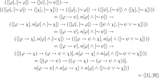
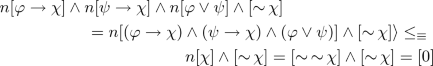
• $\mathsf {E}$(AX2). We need to show that $(\varphi \rightarrow (\psi \rightarrow \chi )) \rightarrow ((\varphi \rightarrow \psi ) \rightarrow (\varphi \rightarrow \chi )) \approx 1$.

  By Theorem 1, it suffices to show that

  

  By Definition 2, it is equivalent to show:

  

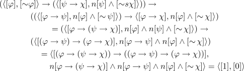
  Since $\mathbf {A}_+$ is a Heyting algebra, $(\varphi \rightarrow (\psi \rightarrow \chi )) \rightarrow ((\varphi \rightarrow \psi ) \rightarrow (\varphi \rightarrow \chi ) \equiv 1$. Moreover, by the fact that n preserves meet and bounds, and $\mathbf {A}_-$ is a Heyting algebra, and the definition of n, we obtain that

  

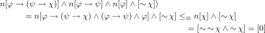
  where $\le _\equiv$ is the lattice order in $\mathbf {A}_-$, and hence $n[\varphi \rightarrow (\psi \rightarrow \chi )] \wedge n[\varphi \rightarrow \psi ]\wedge n[\varphi ] \wedge [\mathop {\sim }\chi ] = [0]$ since [0] is the least element in $\mathbf {A}_-$.

• $\mathsf {E}$ (AX3) and $\mathsf {E}$(AX4). They are immediate consequences of (SN1) and (SN5).

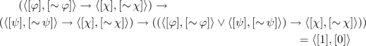
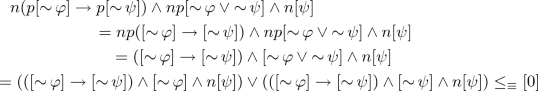
• $\mathsf {E}$(AX5). We need to show that $(\varphi \rightarrow \psi ) \rightarrow ((\varphi \rightarrow \chi ) \rightarrow (\varphi \rightarrow (\psi \wedge \chi ))) \approx 1$.

  By Theorem 1, it suffices to show that

  

  By Definition 2, it is equivalent to show:

  

  Since $\mathbf {A}_+$ is a Heyting algebra, $(\varphi \rightarrow \psi ) \rightarrow ((\varphi \rightarrow \chi ) \rightarrow (\varphi \rightarrow \psi \wedge \chi )) \equiv 1$. Moreover,

  

  By the fact that n preserves meet and bounds, and $\mathbf {A}_-$ is a Heyting algebra, and the definition of n. Hence, $n[\varphi \rightarrow \psi ] \wedge n[\varphi \rightarrow \chi ] \wedge n[\varphi ] \wedge \langle [\mathop {\sim }\psi \vee \mathop {\sim }\chi ]\rangle = [0]$ since [0] is the least element in $\mathbf {A}_-$.

• $\mathsf {E}$(AX6) and $\mathsf {E}$(AX7). They are immediate consequences of (SN1) and (SN5).

• $\mathsf {E}$(AX8). We need to show that $(\varphi \rightarrow \chi ) \rightarrow ((\psi \rightarrow \chi ) \rightarrow ((\varphi \vee \psi ) \rightarrow \chi )) \approx 1$.

  By Theorem 1, it suffices to show that

  

  By Definition 2, it is equivalent to show:

  

  Since $\mathbf {A}_+$ is a Heyting algebra, $(\varphi \rightarrow \chi ) \rightarrow ((\psi \rightarrow \chi ) \rightarrow (\varphi \vee \psi \rightarrow \chi )) \equiv 1$. Moreover,

  

  By the fact that n preserves meet and bounds, and $\mathbf {A}_-$ is a Heyting algebra, and the definition of n. Hence, $n[\varphi \rightarrow \chi ] \wedge n[\psi \rightarrow \chi ] \wedge n[\varphi \vee \psi ] \wedge [\mathop {\sim }\chi ] = [0]$ since [0] is the least element in $\mathbf {A}_-$.

• $\mathsf {E}$(AX9)–$\mathsf {E}$(AX14). They are immediate consequences of (SN6.1), (SN6.2), (SN6.3), (SN6.4), (SN4) and (SN6.5) respectively.

• $\mathsf {E}$(AX15). We need to show that $(\varphi \rightarrow \psi ) \rightarrow (\mathop {\sim }\mathop {\sim }\varphi \rightarrow \mathop {\sim }\mathop {\sim }\psi ) \approx 1$.

  By Theorem 1, it suffices to show that

  

  By Definition 2, it is equivalent to show:

  

  Since $\mathbf {A}_+$ is a Heyting algebra and n preserves meet, $n[\varphi ] \wedge n[(\varphi \rightarrow \psi )] = n[\varphi \wedge (\varphi \rightarrow \psi )] \le _\equiv n[\psi ]$. Hence, $pn[\varphi ] \wedge pn[\varphi \rightarrow \psi ] = pn[\varphi \wedge (\varphi \rightarrow \psi )] \le _\equiv pn[\psi ]$ by p is order-preserving and preserve meet. By residuation law, we obtain that $pn[\varphi \rightarrow \psi ] \le _\equiv pn[\varphi ] \rightarrow pn[\psi ]$, and hence $[\varphi \rightarrow \psi ] \le pn[\varphi ] \rightarrow pn[\psi ]$ since $Id_{\mathbf {A}_+} \le _\equiv pn$, that is, $[\varphi \rightarrow \psi ] \rightarrow (pn[\varphi ] \rightarrow pn[\psi ]) = [1]$. For the other part, since $n[\varphi \rightarrow \psi ] \wedge n[\varphi ] \wedge [\mathop {\sim }\psi ] = n[\varphi \wedge (\varphi \rightarrow \psi )] \wedge [\mathop {\sim }\psi ] \le _\equiv n[\psi ] \wedge [\mathop {\sim }\psi ] = [\mathop {\sim }\psi ] \wedge [\mathop {\sim }\psi ] = [0]$ by the fact that n preserves meet and the definition of n. Therefore, $n[\varphi \rightarrow \psi ] \wedge n[\varphi ] \wedge [\mathop {\sim }\psi ] = [0]$ since [0] is the least element in $\mathbf {A}_-$.

• $\mathsf {E}$(AX16). Since $\varphi \wedge \psi \le \varphi$ by (SN1), we have $\mathop {\sim }\varphi \preceq \mathop {\sim }(\varphi \wedge \psi )$ by (SN5), which is equivalent to $\mathop {\sim }\varphi \rightarrow \mathop {\sim }(\varphi \wedge \psi ) \approx 1$ by (SN2).

• $\mathsf {E}$(AX17)–$\mathsf {E}$(AX22). The arguments are similar as above. All of them are verified by (SN1), (SN5) and (SN2).

• $\mathsf {E}$(AX23). Since $\varphi \wedge (\psi \rightarrow \psi ) \le \varphi$, thanks (SN5) we have $\sim \varphi \preceq \sim (\varphi \wedge (\psi \rightarrow \psi ))$ and by (SN2) follows $\sim \varphi \rightarrow \sim (\varphi \wedge (\psi \rightarrow \psi ))$. The other way around is the same idea, given that $\psi \rightarrow \psi \approx 1$ and $\varphi \le \varphi \wedge (\psi \rightarrow \psi )$.

• $\mathsf {E}$(AX24). We want to prove that $\sim (\varphi \rightarrow \varphi ) \rightarrow \psi \approx 1$. By Theorem 1, it is equivalent to prove that $\langle [\sim (\varphi \rightarrow \varphi ) \rightarrow \psi ], [\sim (\sim (\varphi \rightarrow \varphi ) \rightarrow \psi )] \rangle = \langle [1], [0]\rangle$. Thanks (SN3) we know that $\sim (\varphi \rightarrow \varphi ) \rightarrow \psi \equiv 1$. Regarding $\sim (\sim (\varphi \rightarrow \varphi ) \rightarrow \psi )$, observe that $\sim (\sim (\varphi \rightarrow \varphi ) \rightarrow \psi ) \equiv \sim \sim \varphi \wedge \sim \varphi \wedge \sim \psi$ by (SN4), (SN6.3), (SN6.4) and (SN6.6). Finally $\sim \sim \varphi \wedge \sim \varphi \wedge \sim \psi \equiv 0$ by (SN6.6) and the fact that 0 is the least element.

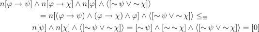
• $\mathsf {E}$(AX25). We need to show that $(\mathop {\sim }\varphi \rightarrow \mathop {\sim }\psi ) \rightarrow (\mathop {\sim }(\varphi \wedge \psi ) \rightarrow \mathop {\sim }\psi )\approx 1$. By Theorem 1 it suffices to show that

  

  By Definition 2, it is equivalent to show:

  

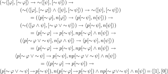
  Since $\mathbf {A}_-$ is a Heyting algebra and p preserves $\rightarrow$ and bounds, $(p[\mathop {\sim }\varphi ] \rightarrow p[\mathop {\sim }\psi ]) \rightarrow (p[\mathop {\sim }\varphi \vee \mathop {\sim }\psi ] \rightarrow p[\mathop {\sim }\psi ]) = p(([\mathop {\sim }\varphi ] \rightarrow [\mathop {\sim }\psi ]) \rightarrow ([\mathop {\sim }\varphi \vee \mathop {\sim }\psi ] \rightarrow [\mathop {\sim }\psi ])) = p [1] = [1]$. Moreover,

  

  since $np = Id_{\mathbf {A}_-}$ and $\mathbf {A}_-$ is a Heyting algebra. Therefore, $n(p[\mathop {\sim }\varphi ] \rightarrow p[\mathop {\sim }\psi ]) \wedge np[\mathop {\sim }\varphi \vee \mathop {\sim }\psi ] \wedge n[\psi ] = [0]$ since [0] is the least element in $\mathbf {A}_-$.

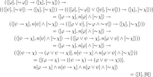
• $\mathsf {E}$(AX26). We need to show that $(\mathop {\sim }\varphi \rightarrow \mathop {\sim }\psi ) \rightarrow ((\mathop {\sim }\chi \rightarrow \mathop {\sim }\gamma ) \rightarrow (\mathop {\sim }(\varphi \wedge \chi ) \rightarrow \mathop {\sim }(\psi \wedge \gamma ))) \approx 1$. By Theorem 1 it suffices to show that

  

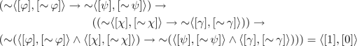
  By Definition 2, it is equivalent to show:

  

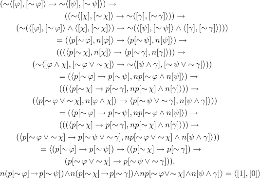
  Since $\mathbf {A}_-$ is a Heyting algebra and p preserves $\rightarrow$ and bounds, $(p[\mathop {\sim }\varphi ] \rightarrow p[\mathop {\sim }\psi ]) \rightarrow ((p[\mathop {\sim }\chi ] \rightarrow p[\mathop {\sim }\gamma ]) \rightarrow (p[\mathop {\sim }\varphi \vee \mathop {\sim }\chi ] \rightarrow p[\mathop {\sim }\psi \vee \mathop {\sim }\gamma ])) = p(([\mathop {\sim }\varphi ] \rightarrow [\mathop {\sim }\psi ]) \rightarrow (([\mathop {\sim }\chi ] \rightarrow [\mathop {\sim }\gamma ]) \rightarrow ([\mathop {\sim }\varphi \vee \mathop {\sim }\chi ] \rightarrow [\mathop {\sim }\psi \vee \mathop {\sim }\gamma ])) = p [1] = [1]$. Moreover,

  

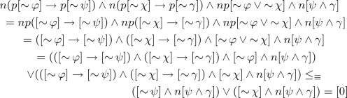
  since $np = Id_{\mathbf {A}_-}$, n preserves meet and $\mathbf {A}_-$ is a Heyting algebra. Therefore, $n(p[\mathop {\sim }\varphi ] \rightarrow p[\mathop {\sim }\psi ]) \wedge n(p[\mathop {\sim }\chi ] \rightarrow p[\mathop {\sim }\gamma ]) \wedge np[\mathop {\sim }\varphi \vee \mathop {\sim }\chi ] \wedge n[\psi \wedge \gamma ] = [0]$ since [0] is the least element in $\mathbf {A}_-$.

2. We have only an inference rule in $\mathbf {QN}$, modus ponens. We need to prove that if $\varphi \approx 1$ and $\varphi \rightarrow \psi \approx 1$, then $\psi \approx 1$ and it follows from transitivity of $\preceq$.

3. We shall prove that if $\varphi \rightarrow \psi \approx 1$, $\psi \rightarrow \varphi \approx 1$, $\mathop {\sim }\varphi \rightarrow \mathop {\sim }\psi \approx 1$, $\mathop {\sim }\psi \rightarrow \mathop {\sim }\varphi \approx 1$, then $\varphi = \psi$. Thanks (SN2) we have $\varphi \preceq \psi$ and $\mathop {\sim }\psi \preceq \mathop {\sim }\varphi$ and therefore by (SN5) follows that $\varphi \le \psi$. Following the same idea we have $\psi \le \varphi$ and being $\le$ the order relation on the lattice we have $\varphi \approx \psi$.

References

Blok, W.J., La Falce, S.B.: Komori identities in algebraic logic. Rep. Math. Logic 34, 79–106 (2000)
Blok, W.J., Pigozzi, D.: Algebraizable Logic, vol. 396. Memoirs of the American Mathematical Society, Providence (1989)
Czelakowski, J., Pigozzi, D.: Fregean logics. Ann. Pure Appl. Log. 127, 17–76 (2004)
Font, J.M.: Abstract Algebraic Logic: An Introductory Textbook. College Publications (2016)
Greco, G., Ma, M., Palmigiano, A., Tzimoulis, A., Zhao, Z.: Unified correspondence as a proof-theoretic tool. J. Log. Comput. 28(7), 1367–1442 (2016)
Greco, G., Liang, F., Palmigiano, A., Rivieccio, U.: Bilattice logic properly displayed. Fuzzy Sets Syst. 363, 138–155 (2019)
Greco, G., Liang, F., Moshier, M.A., Palmigiano, A.: Multi-type display calculus for semi De Morgan logic. In: Kennedy, J., de Queiroz, R.J.G.B. (eds.) WoLLIC 2017. LNCS, vol. 10388, pp. 199–215. Springer, Heidelberg (2017). https://doi.org/10.1007/978-3-662-55386-2_14
Hamilton, A.G.: Logic for Mathematicians. Cambridge University Press, Cambridge (1978)
Liang, F.: Multi-type algebraic proof theory. Dissertation, TU Delft (2018)
Nelson, D.: Constructible falsity. J. Symb. Log. 14, 16–26 (1949)
Palma, C.: Semi De Morgan algebras. Dissertation, The University of Lisbon (2005)
Rivieccio, U., Spinks, M.: Quasi-Nelson algebras. In: Proceedings of LSFA 2018, Fortaleza, Brazil, 26–28 September 2018. Universidade Federal do Ceará (2018)
Rivieccio, U., Spinks, M.: Quasi-Nelson algebras; or, non-involutive Nelson algebras. Manuscript
Sendlewski, A.: Nelson algebras through Heyting ones: I. Stud. Log. 49, 105–126 (1990)
Spinks, M., Rivieccio, U., Nascimento, T.: Compatibly involutive residuated lattices and the Nelson identity. Soft Comput. (2018). https://doi.org/10.1007/s00500-018-3588-9
Vakarelov, D.: Notes on N-lattices and constructive logic with strong negation. Stud. Log. 36, 109–125 (1977)
Wójcicki, R.: Referential semantics. In: Wójcicki, R. (ed.) Theory of Logical Calculi. SYLI, vol. 199, pp. 341–401. Springer, Dordrecht (1988). https://doi.org/10.1007/978-94-015-6942-2_6
Author information
Authors and Affiliations
Corresponding author
Editor information
Editors and Affiliations