Oceanic Tides

Abstract

The phenomena of tides are a matter of common experience: ocean tides under the influence of the Moon and the Sun, differences of the surface level of the oceans reaching several meters, following well-established cycles. In the present chapter we propose a first step in the general and classical mathematical formulations of the tidal potential and tidal force. Then we apply this formulation to the concrete case of the lunisolar ocean tides at a given point of the surface of the sea. At the end we give a review of various tidal manifestations all around the world.

These keywords were added by machine and not by the authors. This process is experimental and the keywords may be updated as the learning algorithm improves.

3.1 Introduction

It is a well-established fact that the origin of the tides is the gravitational action of the Moon and the Sun on objects bound to the Earth [21], but the tidal generating force should not be confused with the gravitational attraction exerted by each of these bodies on the water particles. The tidal generating force is actually the difference between this attraction and what the attraction would be if the particle were located at the center of the Earth. Indeed, the centrifugal force resulting from the orbital motion of the Earth (around the center of mass of the Earth-Moon system or of the Earth-Sun system) is the same at every point of the Earth, while the gravitational attraction varies with the proximity of the celestial bodies according to where the particle is positioned on the surface of the Earth. At the center of mass of the Earth, these two forces balance exactly. Since the Earth radius is small compared with the distance to the Moon (and a fortiori to the Sun), to a first approximation for someone on the Earth surface the magnitude of the force is the same as if the body (Sun or Moon) were at the zenith or the nadir. This explains the semi-diurnal tide (two high tides and two low tides per day). During the day, a maximum force occurs when the Moon crosses the upper semi-meridian and another maximum when it crosses the lower semi-meridian, the minimum occurring when it crosses the horizon (attractive and centrifugal forces are then nearly opposite). However, owing to the inclination of the axis of the Earth’s rotation relative to the axis of the Earth’s orbit, the two extrema are generally not equally pronounced, and sometimes, at higher latitudes, the Sun or the Moon never set or rise (polar night). In this case, a maximum disappears and the resulting type is diurnal (one maximum and one minimum per day). This qualitatively explains some aspects of the tide as described in the preceding paragraph: the generative force of the tide entails diurnal and semi-diurnal components.

In his dynamic theory presented to the Académie Royale des Sciences in 1790, Laplace introduced the concept of tidal generating potential [12]. He was the first to treat the tide as a problem of dynamics of water masses and not as a static problem. According to his dynamic theory, the sea response to the tidal generating force takes the form of extensive waves crossing the oceans with a velocity depending essentially on depths. Moreover, like any wave phenomenon, these waves are reflected, refracted, and diffused according to the nature of the propagation medium and the shape of ocean basins. It follows that the observed tide at any point is the result of the superposition of elementary waves which come from all parts of the ocean, each of them being subject, during its travel, to different propagation conditions. All these components can obviously interfere with one another, resulting in strengthened or attenuated amplitudes according to frequencies.

The hydrodynamic equations of this phenomenon, first formulated by Laplace [13], cannot be easily solved even with modern computing tools available, but they remain the basis of all subsequent developments. Above all, they allow establishing a formula, known as ‘Laplace equation’, applicable to tidal predictions and based on two principles. The first one is that a water mass undergoing a periodic force is subject to a periodic oscillation with the same frequency. The second one is that the total motion of a system subject to small forces is equal to the sum of the elementary motions created by each force.

These two principles express the assumption of the oceans’ linear response to the action of the tidal generating force. It turns out that this assumption is well verified in the case of Brest harbor, where tidal observations were used by Laplace to test his theory. The tidal generating force being divided as a sum of elementary periodic forces, the Laplace equation implies that the tide may itself be decomposed into oscillations of similar periods. The assumption of linearity is not inconsistent with the fact that two parameters, the proportionality factor and the phase shift between the tidal component and corresponding power generator, may depend on the frequency. These parameters also depend on hydraulic conditions of wave propagation, different from one point to another, and in practice must be determined experimentally by analysis of available observations.

The main interest of the Laplace theory lies in its ability to provide a practical method for prediction of high and low tides, known as ‘Laplace method’. In 1839, the hydrographer Chazallon [4] published the first precise scientific timetable of tides based on this method. In this timetable hours and heights of high and low tides at Brest were calculated. For other harbors, they were obtained using time differences and amplitude factors. The Laplace equation has remained the basis of calculation of tides in France for over 150 years. Before the advent of computers, no competing method could indeed claim to provide better accuracy for the calculation of the tide at Brest. However, because of the assumption of linearity, the Laplace equation could not claim to be universally applicable. In fact, they have never been used to calculate the tides at other places than Brest.

Subsequently, we must note the works of two Englishmen, William Whewell [24] (1794–1866) and George B. Airy [1] (1801–1892) [2], who were particularly interested in the propagation of the tidal wave, the first in oceans, the second in canals and rivers, taking friction into account. But we must wait until the late 19th century, with the contribution of Sir William Thomson, better known as Lord Kelvin (1824–1907), to note a real progress in the calculation of tidal predictions [23]. In 1867, the British Association for the Advancement of Science (BAAS) set up a committee to promote the improvement and widespread implementation of the harmonic analysis of tides. The report of this committee was written by Kelvin himself. Some other reports appeared on this subject, but the major contribution was the paper published in 1883 by George H. Darwin (1845–1912) [5]. This paper presents the precise harmonic expansion of the tidal potential, which has been universally used up to the present day as the basis of most studies on tides. Today, the tidal harmonic components are designated by the names assigned by Darwin. In addition, methods of calculation, developed and adapted to the means of that era, were often transposed without changes, even with the technological evolution of computers. However, this development, based on an ancient lunar theory in which all elements are referred to the orbit, was not entirely satisfactory because it is not purely harmonic: it was necessary to introduce correction factors to account for slow changes in the components, mainly due to the slow retrograde motion of the orbit of the Moon. The long-term variations associated with these correction factors can be regarded as constant over periods of the order of one year. Calculated over many years, these factors are available as published tables [22]. The use of these tables is not quite satisfactory for modern computing, but was very useful for manual calculation. That is probably why Darwin remained popular, while as early as 1921 more satisfying purely harmonic expansions such as those proposed by Arthur T. Doodson (1890–1968), were available. Doodson [9] published in the Proceedings of the Royal Society an expansion based on the lunar theory proposed by Brown in 1919 [3]. This new expansion, digital and purely harmonic, provides many more terms than those presented by Darwin and does not require correction factors. Thus tables for these factors were no longer necessary and automatic processing could be greatly improved to come into practical use in the late 1950s. Other expansions, more complete or more accurate, have been proposed since. However, for practical applications in tidal calculations, they do not bring significant progress with respect to the Doodson expansions which remain the reference.

3.2 Basic Mathematical Tidal Theory

In this section we consider the general case of a celestial body orbiting a non rigid planet P. This will give rise to a deformation of this planet. The hypothesis is that this deformation is proportional to the force, to the stress itself. This is why our fundamental aim is to calculate the force exerted on each point P of the planet surface, due to the presence of the celestial body.

Let M be the mass of the non-rigid planet, R its mean radius. O is the position of its center of mass, chosen as origin of the coordinates x, y, z. The celestial orbiting body is regarded as a point mass m, with position Q. While orbiting around O it deforms the planet, and a surface element of the planet is denoted by a position P, at a distance r≃R from the center O.

We introduce the following vector and scalar notation:

3.2.1 Tidal Potential

The potential V calculated at the point P due to the presence of the orbiting body with mass m is given by

(3.1)

with r⋅d=rdcosψ and the gravitational constant.

Let us expand this expression:

(3.2)

Then, if we assume that R≪d,

(3.3)

(3.4)

where P _n represents the Legendre polynomial of degree n.

• V ₀ is a constant term with respect to (x,y,z) and can be dropped,

  

  (3.5)

• V ₁ is the potential corresponding to a system of two masses orbiting around their center of mass,

  

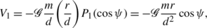  (3.6)

• V ₂ is the first part corresponding to the tidal deformation, which is studied in detail in this chapter,

  

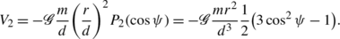  (3.7)

The next term in the expansion would be:

(3.8)

Let us rewrite the amplitude factor A ₂ in V ₂:

(3.9)

where is the gravity at the surface of the planet of mass M, and $\xi= \frac{m}{M} \frac{r^{3} }{d^{3}} r$ depends on the position and mass of the perturbing body.

We recall that the planet is rotating. Consequently it makes sense to speak of its equator and P can be positioned with its latitude φ measured from this equator, and an angle of longitude λ varying with the rotation of the planet. In a similar way the orbiting point mass can be positioned through variable coordinates which are its latitude δ and its longitude λ′.

Now we can introduce the spherical coordinates:

$$ \begin{array}{l@{\qquad}l@{\qquad}l} x= r \cos\varphi \cos\lambda, & y= r \cos\varphi\sin\lambda, & z= r \sin\varphi, \\ u= d \cos\delta \cos\lambda', & v= d \cos\delta \sin\lambda', & w= d \sin\delta. \end{array} $$

(3.10)

They allow us to write:

(3.11)

and consequently,

(3.12)

3.2.2 Tidal Force

From the tide potential V ₂ we can extract the expression for the corresponding tidal force per unit of mass, F ₂, due to the presence of the external body situated at (u,v,w) and acting on the surface point P with coordinates (x,y,z):

$$ \mathbf{F}_2 (x,y,z) = - \mathbf{\nabla}V_2(x,y,z) = \mathbf{\nabla}W_2(x,y,z) = \biggl( \frac{\partial{W_2}}{\partial{x}}, \frac{\partial{W_2}}{\partial {y}}, \frac{\partial{W_2}}{\partial{z}} \biggr). $$

(3.13)

For that purpose, let us rewrite W ₂ in terms of x, y and z:

(3.14)

It is now easy to calculate the three partial derivatives

and the corresponding force per unit of mass, F ₂, acting on P due to Q

(3.15)

We can already analyse the first term, depending on ψ.

• ψ=0 when r and d are aligned: in this configuration, F is maximal and points toward the perturbing body.

• ψ=π when r and d are anti-aligned: in this configuration, F is again maximal but points away from the perturbing body.

Extrapolating these remarks to any point on the surface, we can say that the deformation at any point P of the surface of the planet is instantaneous and directly proportional to the tidal force which creates it. In the case of a deformable planet (like the Earth), the external surface is deformed in such a way that it corresponds to an equipotential surface.

3.3 Expression of the Tidal Potential for the Earth

Here we apply the mathematical principles of the previous section to express the tidal potential V ₂(P) or the associated force function W ₂(P)=−V ₂(P), exerted by an external body (Moon, Sun, planet) with mass m on a point P of the Earth [c??]. P is classically labeled by its spherical coordinates (r,φ,λ), with respect to the terrestrial equator, where φ is the latitude and λ the terrestrial longitude, r being the distance from the center O of the Earth to P.

The position of the perturbing body is given, as before, by its declination δ with respect to the celestial equator and by its longitude λ′, which we replace by its hour angle H defined by H=λ′−λ.

Then the potential W ₂(P) is given by:

(3.16)

(3.17)

We can decompose W ₂ into three terms, named zonal, tesseral and sectorial, which are characterized in the next section, where we make a large use of [c??].

3.3.1 Zonal Part of the Tidal Potential

Let us start with the zonal term, $W_{2}^{\mathit{zonal}}$:

(3.18)

This term is called long period or low frequency because it does not contain the hour angle H, which is by far the highest-frequency variable. Its variations come from the squares of the sines of the declination (sin² δ) of the perturbing body (Moon, Sun, planet) around the Earth, which in reality vary slowly. It introduces a period which is half the time of the relative revolution of the perturbing body, i.e. roughly 14 days in the case of the Moon and 6 months in the case of the Sun. Given the extremal values reached by the declinations, 28^∘30′ for the Moon and 23^∘27′ for the Sun, the last factor is always negative.

The factor $(\sin^{2} \varphi- {1 \over3})$ vanishes at latitudes such that $\sin\varphi= \pm1 / \sqrt{3}$, i.e. at latitudes 35^∘16′N and 35^∘16′S. The locus where this term vanishes are parallels (lines of equal latitude). Taking into account that one factor is always negative, it follows that the long-period term of potential is always positive for latitudes between 35^∘16′N and 35^∘16′S and negative elsewhere.

The partition in zones of latitude of this part of the potential, as it is shown in Fig. 3.1, justifies the terminology of zonal potential.

Fig. 3.1

Zonal distribution of the long period component of the tidal potential

3.3.2 Tesseral Part of the Tidal Potential

The second term $W_{2}^{\mathit{tesseral}}$ is given by:

(3.19)

It is called diurnal, for it contains H with period of roughly one day, regardless of the celestial body m being considered. Its nodes are the meridians normal to the direction of the perturbing body, and the equator (Fig. 3.2). It gives a tesseral structure of equipotential lines, whose sign changes with the declination. The period in the hour angle is approximately 24 hours for the Sun and 24 h 50 min for the Moon. The declination δ and parallax 1/r vary very slowly in comparison to this diurnal frequency.

Fig. 3.2

Tesseral distribution of the diurnal component of the tidal potential

Thus they act as modulations on the diurnal term. The diurnal local maximum is reached when the perturbing body crosses the upper or lower meridian of the observer. The maximal extrema on the Earth are reached at latitudes 45°N and 45°S when δ is itself at its maximum value (23^∘27′ for the Sun and 28^∘30′ for the Moon). The potential is zero for the points at the equator (φ=0^∘) and at the poles (φ=90^∘) or when the declination δ of the orbiting body (Moon, Sun or planet) is zero.

3.3.3 Sectorial Part of the Tidal Potential

Finally the third term $W_{2}^{\mathit{sectorial}}$ is given by:

(3.20)

It is called semi-diurnal, for it contains 2H, with period of roughly 12 h for the Sun and 12 h 25 min for the Moon. Its nodes are the meridians located at 45° of longitude eastward or westward of the meridian containing the perturbing body. These nodes divide the Earth into four sectors. The sectorial potential is positive in the section containing the great circle of the perturbing body and its opposite, and negative in the other two sections.

This is the reason for which it presents a sectoral distribution (Fig. 3.3) over the Earth. This component has two maxima and two minima per day, due to the periodicity of cos2H. The maximal extrema are reached at the equator (φ=0^∘), when the declination of the body (δ) is zero. The semi-diurnal part of the potential is zero at the poles (φ=90^∘).

Fig. 3.3

Sectorial distribution of the semi-diurnal component of the tidal potential

3.3.4 Components of the Local Tidal Force

The local tidal force F=(F _r ,F _φ ,F _λ ) at a given position P can be deduced by simple differentiation of the tidal potential along the three local coordinate axes: the first direction is zenital, the other two directions are horizontal, respectively in the North-South and East-West directions. Let us recall that H=λ′−λ, and then $\frac{\partial {W_{2}}}{\partial{\lambda}}= -\frac{\partial{W_{2}}}{\partial{H}}$. Thus we have, with a relationship similar to Eq. (3.15) but adapted to spherical coordinates:

$$ \mathbf {F} = \mathbf{\nabla}W_2 = \biggl( \frac{\partial {W_2}}{\partial{r}}, \frac{1}{r} \frac{\partial{W_2}}{\partial {\varphi}}, \frac{1}{r \cos\varphi} \frac{\partial {W_2}}{\partial{\lambda}} \biggr). $$

(3.21)

Consequently we have three trigonometric functions: vertical or $\frac {\partial{W_{2}}}{\partial{r}}$, North-South or $\frac{1}{r} \frac {\partial{W_{2}}}{\partial{\varphi}}$, East-West or $\frac{1}{r \cos\varphi} \frac{\partial {W_{2}}}{\partial{\lambda}}$, for each tidal family (zonal, tesseral, sectorial). The nine resulting trigonometric functions characterizing the tidal force are summarized in Table 3.1.

Table 3.1 Trigonometric functions appearing in the expansions of the local tidal force according to the three rectangular directions and the three tidal families

Notice that the deviations of the vertical n ₁ and n ₂ along the two horizontal axes (North-South and East-West) are immediately derived from

$$ n_1 \approx\tan n_1 = {1 \over r g} {\partial W_2 \over\partial \varphi} $$

(3.22)

and

$$ n_2 \approx\tan n_2 = {1 \over r g \cos\varphi} {\partial W_2 \over\partial\lambda}. $$

(3.23)

3.4 Doodson Expansion of the Tidal Potential

The Doodson expansion is based on the theory of the orbital motion of the Moon proposed by Brown (1919) [3], which describes the motion of the Moon in ecliptic coordinates. Brown provided harmonic expansions of the mean longitude, latitude, and the average horizontal parallax of the Moon in a series of trigonometric functions whose arguments are linear in the mean time.

3.4.1 Previous Expansions of the Lunisolar Potential

The expressions of the lunisolar potential given by Laplace [13] in the form of Eqs. (3.18), (3.19) and (3.20) and their derivatives are not directly suitable for the analysis of tidal phenomena because the term 1/d ³ as well as the trigonometric functions containing δ and H exhibit very complicated time-variations due the complexity of the orbital motions of the Earth around the Sun and of the Moon around the Earth.

Laplace already had the idea of expanding the Moon and Sun potentials in sinusoidal functions whose arguments are linear in time. Each term of such an expansion can be understood as the potential of a fictitious body describing a uniform circular motion in the equatorial plane, generating an elementary tidal component with the period of revolution of the fictitious body, and with amplitude and phase depending on the harbor considered. Assuming that the ocean’s response is a linear function of the period of revolution of the Sun and the Moon for diurnal components on one hand and semi-diurnal on the other (i.e. in narrow frequency ranges), Laplace was able to avoid resorting to a purely harmonic expansion. He also showed how to make the potential expansion in a form of purely harmonic components, taking into account the main inequalities of the Moon. Then he deduced the corresponding expressions, independently of any assumption on each component amplitude and phase.

Kelvin [23] and Darwin [6] in 1883 [5] continued Laplace’s work by improving the harmonic expansion of the tidal potential. Darwin’s expansions were the starting point for the harmonic method of calculating tides which have then been used universally [8]. However, the Moon orbital theory available at that time did not allow Darwin to find a comprehensive expansion of the potential. In particular, defects induced by the motion of the lunar nodes were regarded as disturbances requiring the use of correction factors called nodal factors. In 1921, Doodson remedied this situation and published a purely harmonic expansion containing those 386 components whose amplitude coefficient exceeds 10⁻⁴ of the leading one. All the expansions of the tidal potential published after Doodson’s have shown an excellent agreement with them. In the following we explain in detail the principles of construction for Doodson’s series of the tidal potential.

3.4.2 Doodson’s Constant

In the expression of the potential W ₂ in Eq. (3.16) or in Table 3.1, the trigonometric functions are multiplied by the factor , where r and d are respectively the distances of P and of the perturbing body (Moon, Sun, planet) to the center O of the Earth. Therefore it seems judicious to introduce a constant scaling factor close to it [c??].

A natural way of doing this is to replace d by its mean distance c, that is to say its averaged value during a revolution, and to replace r by a radius $\dot{a}$ such that the volume of the sphere of radius $\dot{a}$ is the same as the volume of the Earth. Consequently

$$ \bar{a} = \sqrt[3]{a^2 b} $$

(3.24)

where a and b are respectively the semi-major and semi-minor axis of the Earth (considered as an ellipsoid with a circular equator).

Then we can define the general Doodson’s constant D:

(3.25)

and for the Moon and for the Sun, also called the Doodson’s constants:

(3.26)

Thus the ratio of these two constants is

$$ {D_{S} \over D_{M}} = {m_{S} \over m_{M}} \times{c_{S}^3 \over c_{M}^3} \approx0.4590. $$

(3.27)

This shows why the influence of the Moon on the tides is roughly twice bigger than that of the Sun.

With the help of the Doodson’s constant given by Eq. (3.25), Eqs. (3.18), (3.19) and (3.20) for the potential can be rewritten as

(3.28)

(3.29)

(3.30)

3.4.3 Basic Principle

The three tidal potentials in Eqs. (3.28), (3.29), (3.30) depend on the latitude φ which is constant for a given point P, and on astronomical expansions involving the position of the perturbing body through the variables H, δ, and d. The principle is to truncate the complete expansion to get linear functions of time to approximate the motions, on suitable timescales. Doodson performed this calculations for specific variables which are defined in the next section.

3.4.4 Six Fundamental Variables

The choice of six variables, which over a span of a century may be regarded as linear functions of time, was made by Doodson on the basis of the accumulated results in fundamental astronomy. These variables are:

• τ is the hour angle of the mean Moon shifted by 180°: τ=H _M +180^∘.

• s is the mean tropic longitude of the Moon (‘selene’ is Greek for the Moon).

• h is the mean tropic longitude of the Sun (‘helios’ is Greek for the Sun).

• p is the mean tropic longitude of the lunar perigee.

• N′=−N is the mean tropic longitude of the ascending lunar node with respect to the ecliptic. The sign is changed because N is the only variable decreasing with time.

• p _s is the mean tropic longitude of the Earth perihelion.

All these variables as well as elementary combinations of them are presented together with their period definition (referring to some well-defined astronomical cycle), their hourly angle, and their period, in Table 3.2.

Table 3.2 Main variables involved in the tidal potential with definitions, rates, periods

3.4.5 Preliminary Expansions of Astronomical Trigonometric Functions

3.4.5.1 Lunar Motion

To a first approximation, the orbit of the Moon is quasi-elliptic. However this is too rough when we require more accuracy on its orbital motion, which is especially the case when computing the lunar tidal potential. In fact two main irregularities must be taken into account, respectively called evection and variation.

The evection arises because the Sun crosses twice a year the projection of the semi-major axis of the Moon on the ecliptic (if we neglect the slow motion of the lunar perigee). This results in a gravitational excitation of the eccentricity, its frequency being $(\dot{s} - \dot{p}) - 2 (\dot{h} - \dot{p}) = \dot{s} - 2 \dot{h} + \dot{p}$. The variation arises because the eccentricity of the Moon is modified during the syzygies, when the three bodies (Sun, Earth, Moon) are in conjunction. These two irregularities, due to the perturbing gravitational action of the Sun in the framework of a three body problem, well known as the main problem, affect the ratio c/d and the longitude λ _M , as well as the classical formula of the elliptic motion. We thus have [18]

which gives

$$ \biggl({c_{M} \over d_{M}} \biggr)^3 = 1 + 0.1647 \cos(s-p) + 0.030 \cos(s-2h+p) + 0.024 \cos(2s - 2h) $$

(3.31)

and

In order to use these expansions inside the tidal potential, a last step consists in expressing the declination of the Moon as a function of λ _M :

$$ \sin\delta_{M} = \sin\varepsilon\sin\lambda_{M} = 0.398 \sin \lambda_{M} $$

(3.32)

where ε is the obliquity of the Earth (ε=23^∘27′). It follows that:

(3.33)

(3.34)

(3.35)

3.4.5.2 Solar Motion

In the case of the Sun, the unperturbed elliptic motion is quite acceptable:

$$ {c_{S} \over d_{S}} = 1 + e_{\mathit{Earth}} \cos(h - p_s) = 1 + 0.0167 \cos(h - p_s) $$

(3.36)

which gives

$$ \biggl({c_{S} \over d_{S}} \biggr)^3 = 1 + 0.0502 \cos(h - p_s) + \cdots $$

(3.37)

and, for the longitude,

$$ \lambda_{S} = \dot{h}_0 t + 0.0335 \sin(h-p) t. $$

(3.38)

The expression for cos² δ _S involves the same coefficients as for the Moon in Eq. (3.34):

$$ \cos^2 \delta_{S} = 0.921 + 0.0792 \cos2 h + \cdots $$

(3.39)

3.5 Tidal Spectrum

Now that we have obtained the necessary expansions of the trigonometric functions of astronomical angles involved in the tidal potential W ₂, it is possible to express each part of W ₂ (sectorial, tesseral, zonal) as a combination of sinusoidal functions whose arguments are expressed themselves as combinations of the Doodson’s variables.

3.5.1 Characterization of the Semi-diurnal Waves

The semi-diurnal (or sectorial) waves come from the sectorial part of the potential given by Eq. (3.30).

3.5.1.1 Lunar Sectorial Part

In the case of the Moon, H _M =τ−180^∘, and by using the expansion of (c _M /d _M )³ and cos² δ _M respectively given by Eqs. (3.31) and (3.34), we get:

(3.40)

(3.41)

The result is an infinite number of terms which show frequencies symmetrically distributed on both sides of the half lunar-day frequency. The leading oscillation is obviously 0.921Dcos² φcos2τ. It is classically called the M₂ wave and its period is the mean lunar day, that is to say 12^h25^min14^s. The following biggest wave is called N₂ with argument 2τ+(s−p) associated with a symmetrical wave with much smaller amplitude and argument 2τ−(s−p). Another big wave is named K_2M with argument 2τ+s which corresponds to the sidereal day. The index M stands for ‘Moon part’, as this wave is also present in the case of the solar part.

3.5.1.2 Solar Sectorial Part

In a way similar to what was done above for the lunar part, we take into account that the hour angle of the Sun is H _S =τ+s−h and we use the expansions of (c _S /d _S )³ and cos² δ _S respectively given by Eqs. (3.37) and (3.39). We get:

(3.42)

(3.43)

The leading wave with argument 2τ+2s−2h has a half mean solar-day period, that is to say exactly 12^h00^min00^s and is called S₂. Other main oscillations are called elliptic or declinational because they come either from the ellipticity of the Earth orbit or from the declination of the Sun. The leading waves of the first category are named R₂ and T₂ with respective symmetrical arguments 2τ+2s−2h−(h−p _S ) and 2τ+2s−2h+(h−p _S ), those of the second category have arguments 2τ+2s−2h+2h (named K_2S) and 2τ+2s−2h−2h.

3.5.2 Characterization of the Diurnal Waves

The diurnal (or tesseral) waves come from the sectorial part of the potential given by Eq. (3.29).

3.5.2.1 Lunar Tesseral Part

Still by taking H _M =τ−180^∘, and by using the expansion of (c _M /d _M )³ and sin2δ _M respectively given by Eqs. (3.31) and (3.33), we get

(3.44)

(3.45)

In contrast with the semi-diurnal part, a leading oscillation with no symmetrical counterpart does not exist because the mean value of sin2δ _M is zero (there is no constant part in the second term of the right hand side). Thus the leading oscillations are the two symmetrical declinational waves K_1M which corresponds to the sidereal day with argument τ+s and period 23^h56^min04^s, and O₁ with argument τ+s and period 23^h49^min10^s.

3.5.2.2 Solar Tesseral Part

By analogy with the lunar part and taking into account that H _S =τ+s−h we have:

(3.46)

As for the Moon we find the term K₁ (called here K_1M) with a sidereal day period, and argument τ+s (or t+h), coming from the combinations of the terms with argument h and τ+s−h and its symmetric counterpart, with argument τ+s−2h (or t−h).

3.5.3 Characterization of the Long Periodic Waves

The long periodic (or zonal) waves come from the zonal part of the potential given by Eq. (3.28).

3.5.3.1 Zonal Lunar Part

The lunar zonal part is written

$$ \bigl(W_{2}^{\mathit{zonal}} \bigr)_{M} = 3 D_{M} {c_M^3 \over d_M^3} \biggl( \sin^2 \varphi- {1 \over3} \biggr) \biggl(\sin^2 \delta_M - {1 \over 3} \biggr). $$

(3.47)

By using the expansions of (c _M /d _M )³ and cos² δ _M from Eqs. (3.31) and (3.34) and after combining the trigonometric functions,

(3.48)

Thus the main zonal lunar oscillation has an argument 2s and a semi-monthly (fortnightly) period 13.66 d. It is called M_f (Moon, fortnightly). The second most important term is named M_m (Moon, monthly) with argument s−p which corresponds to the anomalistic month.

3.5.3.2 Zonal Solar Part

The solar zonal part is written

$$ \bigl(W_{2}^{\mathit{zonal}} \bigr)_{\mathit{Sun}} = 3 D_{\mathit{Sun}} {c_S^3 \over d_S^3} \biggl( \sin^2 \varphi- {1 \over3} \biggr) \biggl(\sin^2 \delta_S - {1 \over3} \biggr). $$

(3.49)

We use the expansion

(3.50)

The dominant term here is a semi-annual wave with argument 2s and period 182.62 d and an annual one with argument h−p _S corresponding to the anomalistic year with period 365.26 d.

3.5.4 Catalogue for the Lunisolar Potential

Of course it is possible to expand the lunisolar potential into an infinite series of sinusoidal terms. The number of terms taken into account expresses the level of truncation. George Darwin (1883) kept 91 terms, Doodson [9] kept 378 terms, and Hartmann and Wenzel [11] kept 12 935 waves in their catalogue, called HW95, including 1 483 waves due to the direct planetary effects. These last authors did their calculations with DE200 numerical ephemerids of the planets and the Moon, between the years 1850 and 2150.

In Table 3.3 we present the principal tidal waves. We have separated the lunar waves form the solar ones. The coefficients are those coming from Doodson’s expansion, very close to those calculated by Darwin. In practice, only their relative magnitudes are considered.

Table 3.3 Main components of the lunisolar tides

This table requires some comments:

• The coefficients of Sa and S1 are very weak: these components should not be included because there exist other more important components which are not mentioned. They are introduced to take into account the annual and diurnal height variations of tidal observations, of meteorological origin.

• As already mentioned, the components K1 and K2, sometimes called ‘sidereal components’ since their periods equal respectively the sidereal day and the half-sidereal day, are present in both the solar potential and the lunar potential. For all studies concerning these components, the coefficients to consider are the sum of the coefficients coming from both sources.

• The constant terms obviously do not intervene in the tide. The long period components are usually very weak. They are often masked by noise of meteorological origin and are not easily detected in tidal observations. Only components Sa and Ssa, reflecting seasonal variations in the sea level can generally be identified.

• The diurnal main components are K1, O1, P1, Q1, and the main semi-diurnal ones are M2, S2, K2, N2. They contain the main part of the tidal signal energy and are the only waves generally taken into account in the first approximation for quick studies.

3.6 Tidal Behavior and Predictions Around the World

In terms of tidal prediction, through Doodson’s work in particular, the harmonic method has provided a practical, precise and potentially universal tool. It is not fundamentally different from Laplace’s method for it too relies on a theoretical formulation including a number of fixed parameters which must be determined experimentally by analyzing the available observations. For a good accuracy, these observations must extend over a sufficiently long time. Generally, a year of hourly measurements is necessary to achieve the accuracy required for the purposes of navigation. Moreover the results are useful only for the site where observations have been made.

A more ambitious approach, based on the hydrodynamics of ocean basins, had been proposed since a long time ago, by such pioneers as Bernoulli, Whewell, Poincaré, and Harris. However given the complexity of bathymetry and coastlines, it was not possible to obtain an accurate solution to the problem of tide modeling until powerful computing resources came into existence. Analytical solutions are nevertheless capable of explaining qualitatively the main features of tide propagation, for example the existence of amphidromic points. However it was the development of numerical methods, becoming possible with the ever improving computers, that really allowed progress in this direction. In particular, the work of the German specialist Hansen (1949) has been the source of new attempts to solve the Laplace equation for the real ocean [10].

It should be noted that altimetry from satellite tracking and geodesy have created new needs for an elaborate knowledge of tides and have led to a renewed interest in world ocean modeling. In particular, satellite altimetry, which measures the sea-level with a quasi-centimeter accuracy, has enabled the development of much more realistic tidal models by assimilating always more abundant data.

3.6.1 Global Characteristics

Laplace described the tides as ‘the most difficult problem of all celestial mechanics’. The complexity of this phenomenon lies primarily in its description. The more we want to refine it, the more we realize that some empirical rules can be established from partial observations, which can only be coarsely generalized. It is very difficult indeed to detect a temporal ‘rhythm’ in tidal phenomena. It is even theoretically impossible because, in contrast to common belief, the tides are not periodic: there is no period after which the height variations repeat exactly the same way. Indeed, there are periods after which the same conditions are almost fulfilled, the best known being the Saros, equal to 223 lunar months, or 6585.32 days. After this time interval, the Moon, the Sun are nearly in the same relative positions and their orbital elements are also nearly the same. It follows that the tidal generating force takes nearly the same value. This does not mean that the Saros is a period of tides: after several Saros, the resemblance with the initial tide diminishes further and further.

3.6.2 Tide Amplitudes in the Oceans

Besides the difficulties of temporal description of the tides, a spatial description presents another set of difficulties. In terms of height first, the geographical distribution of amplitudes in the oceans (Fig. 3.4) seems to follow no obvious a priori pattern. However, we can note that the highest amplitudes are mainly located on continental shelves around the continents, or in shallow seas such as the English Channel. These amplitudes are very weak in semi-enclosed seas of small size (Sea of Japan, Caribbean, Baltic, Mediterranean). Apart from these qualitative observations implying the effect of depth and size of oceanic basins, no general rule can be established.

Fig. 3.4

Tidal amplitudes of oceans worldwide

3.6.3 Tide Characterization

As we have shown in the previous section, the tides are mainly due to the superposition of a diurnal component (daily maximum and minimum height) and a semi-diurnal component (two maxima and two minima per day). Nevertheless, the relative importance of these two components varies geographically, defining types, according to a more or less conventional classification:

• a semi-diurnal type characterized by a negligible component of the diurnal tide,

• a semi-diurnal type with diurnal inequality: the semi-diurnal component is dominant but is modified by the diurnal one,

• a mixed type: the diurnal component dominates, but is modified by the semi-diurnal one,

• a diurnal type: the semi-diurnal component is negligible.

The distribution of these 4 types of tide in the ocean worldwide (Fig. 3.5) shows that no general rule can be established, apart the observation that the semi-diurnal type is dominant in the Atlantic, the other types appearing only when the semi-diurnal amplitude is low.

Fig. 3.5

Types of the dominating tides in the oceans all around the world

3.6.4 Amphidromic Points

Another feature of the tide is its mode of spreading. The crests of each wave component propagate around points called amphidromic points.¹ These points occur because of the combined action of the Coriolis force and the interference with oceanic basins, seas, and bays. Each tidal component is at the origin of a different amphidromic system. Amphidromic points for a tidal constituent (diurnal, semi-diurnal, etc.) is characterized by the property that there is almost no vertical motion of the oceanic mass from tidal action. Nevertheless tidal currents can appear when water levels on two sides of the amphidromic point are not the same. This leads to a well-defined wave pattern called an amphidromic system.

In the example of a semi-diurnal pattern spread in the Atlantic Ocean shown in Fig. 3.6, each line, called co-tidal line, indicates the position of the crest of the wave at a given hour, referred to the transit of the Moon at the Greenwich meridian. We can note for example that the wave progresses from south to north along the coasts of Europe, but from north to south along the North American coast. The rotation around an amphidromic point does not seem to follow any general rule: for example, the two major networks of the South Atlantic rotate in opposite directions. These co-tidal lines, representing the average semi-diurnal tide, does not exactly match the actual tide. Amphidromic points are not absolutely fixed, and it would be wiser to speak of amphidromic area. In addition, the diurnal component propagates very differently: the corresponding number of amphidromic points is approximately half in the case of the semi-diurnal component. All these tidal characteristics, with gradually more precise and abundant data, have long been subject to questions, hypotheses (often fallacious), theoretical developments, and scientific studies conducted with the help of technologies becoming more sophisticated and more adequate in particular thanks to the innovation of artificial satellites and powerful computers.

Fig. 3.6

Co-tidal lines in Atlantic Ocean

3.6.5 Tidal Curves

The graph versus time of sea level measurements or predictions at a given surface point of the ocean is called a tidal curve. As an example, we show in Fig. 3.7 the tidal curve obtained from observations at Brest of the semi-diurnal tide for one day time span. Each minimum of the curve is called low tide and each maximum high-tide. From the low tide to the high tide, the sea level rises during the flow phase, and decreases from high to low during the ebb phase. The difference between the high tide level and the low tide one is called the tidal range, not to be confused with the amplitude, which is the norm of a sinusoidal function. Nevertheless the word ‘amplitude’ is sometimes used for the tide, for which it means ‘half the tidal range’. The heights are referred to a reference level which often comes from a nautical chart.

Fig. 3.7

Tidal curve observations at Brest

Figure 3.8 shows another example of the semi-diurnal tide curve deduced from a prediction for roughly thirty days. At the times of new and full Moon, the lunar- and solar-induced ocean bulges line up (and add up) to produce tides having the highest monthly tidal range (i.e. the highest high tide and the lowest low tide): they are called the spring tides. In the opposite case, at the first and third quarter phases of the Moon, the Sun’s pull on the Earth is at right angles to the Moon’s pull. At this time tides have their minimum monthly tidal range (i.e. unusually low high tide and unusually high low tide). These are called the neap tides or fortnightly tides.

Fig. 3.8

Semi-diurnal tides with range variations during one month at Brest

Changes in tidal range are generally recorded from a minimum (neap tide) to a maximum (spring tide). The alternative phases of increasing and decreasing tidal ranges are called respectively revival and waste. The time interval between one phase as a full Moon or a new Moon, and the tidal extremum which follows immediately, is called the age of the tide.

3.6.6 Tidal Curves According to Tidal Types

As mentioned before, the distinction between types of tides is somewhat conventional. A classification into three types is often suggested, but the classification in four types corresponding already defined in Sect. 3.6.3 (see Fig. 3.5) is proposed hereafter, where we show in Fig. 3.9 four different tidal behaviors on the Earth.

Fig. 3.9

The four types of tides: examples of Casablanca (semi-diurnal), Vung Tau (semi-diurnal with diurnal inequality), Qui Nhon (mixed) and Do Son (diurnal)

3.6.6.1 Semi-diurnal Tide (Casablanca, Morocco)

This type of tide has been presented before (Fig. 3.8). It exhibits every day two high tides and two low tides of nearly the same level, with nearly equal tidal ranges throughout the daytime. This type of tide dominates in the Atlantic, especially in Europe and Africa. However, as has been noted above, other types of tide are likely to be encountered.

3.6.6.2 Semi-diurnal Tide with Diurnal Inequality (Vung Tau, Vietnam)

During a lunar day, two relatively small tidal ranges are followed by two larger tidal ranges, or vice versa. The difference between large and small tidal ranges, called the diurnal inequality, is maximized when the declinations of the Moon and the Sun are themselves close to their maximum. The diurnal inequality is also observed on European coasts, although the tide is characterized as semi-diurnal, for the diurnal inequality is small. However, it may be very important in many ports in the Pacific and Indian Oceans.

3.6.6.3 Mixed Tide (Qui Nhon, Vietnam)

Mixed tide is characterized by the succession of a semi-diurnal type and a diurnal type during a lunar month. This type of tide is common in Indonesia, Indochina, on the coasts of Siberia, and Alaska. It is also found in the Atlantic Ocean and the Caribbean Sea.

3.6.6.4 Diurnal Tide (Do Son, Vietnam)

Diurnal tide presents only one high tide and one low tide per lunar day, with a tidal range varying with the declinations of the Moon and the Sun. This type of tide, rather uncommon, is observed mainly in the Pacific Ocean: in Siberia (with very large ranges), in Alaska and also in Southeastern Asia.

3.6.7 Tides in Shallow Water

When propagating through shallow water, almost all primitively sinusoidal deep-water offshore tides are deformed. The periodic components, issued from the generating force, combine themselves through nonlinear processes, creating harmonics which can propagate independently. The tidal curves observed in the English Channel and the North Sea coasts (Fig. 3.10) are typical examples of tidal curves after a long progression of the tidal wave over a shallow shelf.

Fig. 3.10

Shallow water tidal waves in the Channel at Portsmouth (above) and in the North Sea at Hoek Van Holland (below)

The propagation in estuaries exhibits other examples of distortion of the tidal wave in shallow water. This kind of deformation is related to the laws of hydrodynamics, which states that the speed of a hydraulic wave is proportional to the square root of the depth. In deep water, the difference of magnitude does not alter the speed of propagation. On the contrary in shallow water, the peak of the wave moves faster than the trough, so that a wave crest tends to overtake the preceding wave. The example of the Gironde estuary in Fig. 3.11 is telling of such a behavior.

Fig. 3.11

Tidal curves in the Gironde estuary

In extreme cases it forms a bore, a water bar moving upstream along a river. This phenomenon is present in many estuaries of major rivers. The height of the bar can reach several meters, especially in the estuary of the Amazon, the Hoogly and Indus rivers in India and the Tsien Tang in China.

3.6.8 Spectral Characteristics of Tides

The tidal spectrum, despite being the result of a calculation, is really an objective mode of representation of tidal phenomena, independent of any theory. It is particularly suited to tidal studies. It is not necessary to give an exact definition of the spectrum. It only matters that it represents the amplitude, or energy, as a function of frequency.

In Fig. 3.12 we present the spectra at two points of the Loire estuary. They are characterized by a low resolution, which means that there is an imperfect separation of adjacent frequencies. The comparison between the two spectra shows the evolution of the structure from the mouth of the river to upstream. These examples show that the main characteristic of the tidal spectrum is split into separate, regularly spaced clusters. The main group is the semi-diurnal one (two cycles per lunar day).

Fig. 3.12

Semi-diurnal tidal spectrum at Saint-Nazaire at the mouth of the Loire estuary and at Nantes, about 100 km upstream

It is worth noting that the energy increases as the frequencies decreases. A significant noise originates from atmospheric influences. Figure 3.12 shows also the increase of the number of harmonics when the tidal wave progresses from the mouth of the Loire to Nantes, located one hundred miles upstream. The upstream spectrum shows presence of energy in high frequencies. Indeed, only the first 3 groups (diurnal, semi-diurnal, and third-diurnal) represent the bulk of the astronomical tide issued directly from the actions of the Moon and the Sun. Other groups appear during the progress of the tidal waves in shallow waters.

After analyzing more than 120 years of almost continual observations, the spectral signature at high resolution of the semi-diurnal group in Brest (Fig. 3.13) exhibits thin, well separated components, justifying (retrospectively) the representation of tide as harmonic series. An even better illustration is given in Fig. 3.14, which presents the expansion of the spectrum close to the M2 component. The main components, clearly identified, are named after Darwin (or Doodson).

Fig. 3.13

High resolution semi-diurnal spectrum at Brest

Fig. 3.14

High resolution M2 group

3.6.9 Tidal Currents

We can consider that any tide is an oscillation similar to a swell. In both cases, water molecules approximately describe closed trajectories in a vertical plane. However, unlike swell, the tide wavelength is always greater than the depth. In a homogeneous and deep ocean, tidal motions affect the whole depth of water. All molecules of a given vertical plane describe extremely flattened orbits. The vertical motion is the tide, whereas the horizontal motions, incomparably more prominent, constitute the tidal currents.

In a density stratified ocean, internal tidal waves are created, especially near continental slopes. They change the vertical structure of currents. In extreme cases, as in the Strait of Gibraltar, for instance, the currents caused by these internal waves, mainly semi-diurnal, may be opposite in direction between the surface and the bottom. Moreover the energy dissipation of tides is mainly due to current friction at the bottom. The study of currents may be conducted with the same tools as the study of tides, but it is more difficult at least for two reasons: first, because of the large spatial variability of their characteristics from one point to another and, second, because of the much more important influence of atmospheric factors. Strong tidal currents in some areas justify their study in order to provide valuable help to sailors, which constitutes an important activity of hydrographic offices. Figure 3.15 shows results of the modeling of tidal currents around the island of Batz (France). It comes from a navigation aid document, particularly useful in some areas where tidal currents are sometimes violent.

Fig. 3.15

Model of tidal currents around the island of Batz (France)

References

Airy, G.B.: Tides and waves. In: Rose, H.J. et al. (eds.) Encyclopaedia Metropolitana. Mixed Sciences, vol. 3, pp. 1817–1845 (1841)
Airy, G.B.: Tides and waves. In: Encyclopedia Metropolitana, vol. 5, pp. 241–396. London (1845)
Brown, E.W.: Tables of the Morion of the Moon. Yale University Press, New Haven (1919)
Chazallon, M.: Annuaire des marées des cotes de France. Dépot des Cartes et Plans, Paris (1839)
Darwin, G.H.: Report on the harmonic analysis of tidal observations. Brit. Assoc. Rep, pp. 49–117 (1883)
Darwin, G.W.: On the figure of equilibrium of a planet of heterogeneous density. Proc. R. Soc. Lond. 1(36), 158–166 (1883)
Darwin, G.: On tidal prediction. Proc. R. Soc. Lond. 49, 130–133 (1890)
Darwin, G.H.: The harmonic analysis of tidal observations. In: Scientific Papers, vol. 1, pp. 1–70. Cambridge University Press, Cambridge (1907)
Doodson, A.T.: Harmonic development of the tide-generating potential. Proc. R. Soc. Lond. Ser. A 100, 305–329 (1921)
Hansen, W.: The Reproduction of the Motion in the Sea by Means of Hydrodynamical Numerical Methods. Pub. N∘5, pp. 1–57. Mitteilung Inst. Meereskunde, Univ. Hamburg, Hamburg (1966)
Hartmann, T., Wenzel, H.G.: The HW95 tidal potential catalogue. Geophys. Res. Lett. 22(24), 3553–3556 (1995)
Laplace, P.S.: Mémoire sur le flux et le reflux de la mer. Mém. Acad. Sci., pp. 45–181 (1790)
Laplace, P.S.: Traité de mécanique céleste, vol. 2, livre 4 (1799); vol. 5, livre 13 (1825)
Le Provost, C., Genco, M.L., Lyard, F., Canceil, P.: Spectroscopy of the world ocean tides from a finite element hydrodynamic model. J. Geophys. Res. 99(C12), 24777–24797 (1994)
Lubbock, J.W.: On the tides. Philos. Trans. R. Soc. Lond. 127, 97–104 (1837)
Marchuk, G.I., Kagan, B.A.: Dynamics of Ocean Tides. Kluwer, Dordrecht (1989), 327 pp
Mazzega, P.: The M2 ocean tide recovered from seasat altimetry in the Indian ocean. Nature 302, 514–516 (1983)
Melchior, P.: The Tides of the Planet Earth, 2nd edn. Pergamon, Elmsford (1982), 641 pp
Munk, W.H., Cartwright, D.E.: Tidal spectroscopy and prediction. Philos. Trans. R. Soc. Lond. A 259, 533–581 (1966)
Munk, W.H., MacDonald, G.J.F.: The Rotation of the Earth—A Geophysical Discussion. Cambridge University Press, Cambridge (1960), 323 pp
Newton, S.I.: Principia. University of California Press, Berkeley (1687)
Schuremann, P.: Manual of harmonic analysis and prediction of tides (1971); U.S. Coast and Geodetic Survey (1971)
Thomson, W.: On gravitational oscillations of rotating water. Proc. R. Soc. Edinb. 10, 92–100 (1879)
Whewell, W.: Researches on the Tides, 14th series. On the Results of Continued Tide Observations at Several Places on the British Coasts, pp. 227–233
Author information
Authors and Affiliations
Corresponding author
Editor information
Editors and Affiliations
Rights and permissions
Copyright information
© 2013 Springer-Verlag Berlin Heidelberg
About this chapter
Cite this chapter
Simon, B., Lemaitre, A., Souchay, J. (2013). Oceanic Tides. In: Souchay, J., Mathis, S., Tokieda, T. (eds) Tides in Astronomy and Astrophysics. Lecture Notes in Physics, vol 861. Springer, Berlin, Heidelberg. https://doi.org/10.1007/978-3-642-32961-6_3
Download citation
DOI: https://doi.org/10.1007/978-3-642-32961-6_3
Publisher Name: Springer, Berlin, Heidelberg
Print ISBN: 978-3-642-32960-9
Online ISBN: 978-3-642-32961-6
eBook Packages: Physics and AstronomyPhysics and Astronomy (R0)