
Abstract
In decision and risk analysis problems, modelling uncertainty probabilistically provides key insights and information for decision makers. A common challenge is that uncertainties are typically not isolated but interlinked which introduces complex (and often unexpected) effects on the model output. Therefore, dependence needs to be taken into account and modelled appropriately if simplifying assumptions, such as independence, are not sensible. Similar to the case of univariate uncertainty, which is described elsewhere in this book, relevant historical data to quantify a (dependence) model are often lacking or too costly to obtain. This may be true even when data on a model’s univariate quantities, such as marginal probabilities, are available. Then, specifying dependence between the uncertain variables through expert judgement is the only sensible option. A structured and formal process to the elicitation is essential for ensuring methodological robustness. This chapter addresses the main elements of structured expert judgement processes for dependence elicitation. We introduce the processes’ common elements, typically used for eliciting univariate quantities, and present the differences that need to be considered at each of the process’ steps for multivariate uncertainty. Further, we review findings from the behavioural judgement and decision making literature on potential cognitive fallacies that can occur when assessing dependence as mitigating biases is a main objective of formal expert judgement processes. Given a practical focus, we reflect on case studies in addition to theoretical findings. Thus, this chapter serves as guidance for facilitators and analysts using expert judgement.
Access provided by CONRICYT-eBooks. Download chapter PDF
8.1 Introduction
Probabilistic modelling of uncertainties is a key approach to decision and risk analysis problems. It provides essential insights on the possible variability of a model’s input variables and the uncertainty propagation onto its outputs.
Typically, uncertainties cannot be treated in isolation as they often exhibit dependence between them which can have unanticipated and (if not properly modelled) possibly misleading effects on the model outcome. Therefore, modelling dependence of uncertainties is an area of ongoing research and several modelling approaches have been developed, serving different purposes and allowing for varying levels of scrutiny. A common challenge with regards to model quantification is a lack of relevant historical data while simplifying assumptions, such as that of independence, are not justifiable. Then, the only sensible option for quantifying a model is by eliciting the dependence information through expert judgement. This is even necessary when relevant data on the marginal probabilities are available.
A structured approach to eliciting multivariate uncertainty is encouraged as it supports experts to express their knowledge and uncertainty accurately, hence producing well-informed judgements. For instance, cognitive fallacies might be present when experts assess dependence which can inhibit the judgements’ accuracy. Therefore, mitigation of these fallacies is a main objective of an elicitation process. Further, a structured process addresses other questions which affect the reliability of the elicited result and hence model outcome, such as aggregating various judgements. Lastly, a formal process makes the elicited results transparent and auditable for anyone not directly involved in the elicitation.
8.1.1 Objective and Structure of the Chapter
Complementary to the case of eliciting univariate uncertainty, this chapter’s objective is to outline the main elements of formal expert judgement processes for multivariate uncertainty elicitation. This is done by discussing theoretical and empirical findings on the topic, though the reader should note that fewer findings are available for eliciting joint distributions than for the elicitation of univariate quantities.
The structure of this chapter is as follows. In the remainder of this section we introduce a definition of dependence for the subjective probability context which establishes a common language and understanding of the key concept discussed here. In Sect. 8.2, the importance of formal expert judgement processes is discussed and an overview of the necessary adjustments for dependence elicitation is given. This provides the reader with the scope of the topic. Section 8.3 outlines the heuristics and biases that might occur when eliciting dependence. Then, Sect. 8.4 discusses the preparation of an elicitation (or the pre-elicitation stage) which for instance entails the choice of the elicited forms and the training of experts. In Sect. 8.5, we present considerations for the actual elicitation phase, including structuring and decomposition methods as well as the quantitative assessment. In Sect. 8.6, we review required alterations of the process for the post-elicitation stage, such as when combining the expert judgements. Finally, Sect. 8.7 concludes the chapter by summarising the main points addressed and discussing the status-quo of this research problem.
8.1.2 Dependence in the Subjective Probability Context
In this chapter, we use the terms dependence and multivariate uncertainty interchangeably and in a general sense. They contrast the specific association measures (or dependence parameters) that quantify a dependence model and are therefore often used as elicited variables. When discussing dependence in a general sense, we refer to situations with multiple uncertain quantities and when gaining information about one quantity, we change the uncertainty assessments for the others. More formally, we say that two uncertain quantities X and Y are independent (for experts) if they do not change their beliefs about the distribution of X after obtaining information about Y. This is easily extended to higher dimensions in which all quantities are independent of one another if knowing about one group of variables does not change experts’ beliefs about the other variables. It follows that dependence is simply the absence of independence.
Note that dependence in a subjective probability context is a property of an expert’s belief about some quantities so that one expert’s (in-)dependence assessment might not be shared with another expert who possesses a different state of knowledge (Lad 1996).
8.2 Structured Expert Judgement Processes: An Overview
The necessity for a structured and formal process when eliciting uncertainty from experts, such as in form of probabilities, has been recognised since its earliest approaches. For instance, it has been acknowledged in the area of Probabilistic Risk Analysis (PRA) which comprises a variety of systematic methodologies for risk estimation with uncertainty quantification at its core (Bedford and Cooke 2001). From a historical perspective, main contributions in PRA have been made in the aerospace, nuclear and chemical process sector. Hence, after expert judgement was used only in a semi-formal way in one of the first full-scale PRAs, the original Reactor Safety StudyFootnote 1 by the US Nuclear Regulatory Commission (USNRC 1975), major changes towards a more scientific and transparent elicitation process were made in the subsequent studies, known as Nureg-1150 (USNRC 1987; Keeney and Von Winterfeldt 1991). When reflecting on the historical development of PRA, Cooke (2013) highlights the improvements made through a traceable elicitation protocol as a newly set standard and main achievement for expert judgement studies.
Another pioneering contributor to formal approaches for expert judgement is the Stanford Research Institute (SRI). The Decision Analysis Group of SRI similarly acknowledged the importance of a formal elicitation process when eliciting uncertainty from experts. Therefore, they developed a structured elicitation protocol that supports a trained interviewer through a number of techniques to reduce biases and aid the quantification of uncertainty (Spetzler and Staël von Holstein 1975; Staël von Holstein and Matheson 1979).
Following from these early contributions, various proposals for formal expert judgement processes have been made and its various components were further developed. While not one particular step-by-step process to follow exists given the varying and particular objectives of each elicitation, there is agreement regarding which high level steps are essential. Fairly complete elicitation protocols are for instance presented in Merkhofer (1987), Morgan and Henrion (1990), Cooke and Goossens (1999), Walls and Quigley (2001), Clemen and Reilly (2014) and EFSA (2014). Even though these references explicitly address the case of eliciting a univariate quantity, they serve as guidance for our purpose of presenting and discussing the considerations for eliciting dependence.
The elicitation of dependence follows historically from advances made for eliciting univariate uncertainty and an overview of the historical development of expert judgement in risk analysis is presented in Cooke (2013). This development is not surprising given that marginal distributions need to be specified (at least implicitly) before any dependence assessment can be made. Furthermore, univariate quantities are (typically) more intuitive to assess. Whereas some findings for eliciting univariate uncertainty are still applicable in the multivariate case, for other parts of the process adjustments need to be made. Figure 8.1 shows the main elements of elicitation processes with the modifications that are necessary when eliciting dependence.

Overview of the expert judgement process adjusted for eliciting dependence (steps discussed in this chapter are in grey)
Regarding the different roles during an elicitation, in this chapter we consider the situation of a specific decision or risk analysis problem that is of importance for a decision maker. Experts assess the uncertainty on the variables without any responsibility for the model outcome or consequences of the later decision. The experts are chosen based on their substantive (also subject-matter) expertise, meaning they are experts on the particular topic of the decision problem. This implies that the experts might not have normative expertise, thus they are not statistical or probabilistic experts. The facilitator, who manages the actual elicitation part of the overall process, might be either the same person as the decision maker or an independent third type of attendee at the elicitation workshop. The facilitator clarifies any questions from the experts. An analyst on the other hand is usually in charge of the whole process. This includes the preparation of the elicitation and the finalisation of results afterwards. Such a situation with a given, formulated problem and clearly defined roles is often the case, however other ones are possible. French (2011) discusses various elicitation contexts and their potential implications.
We regard an elicitation as successful if we can be confident that the experts’ knowledge is captured accurately and faithfully, thus their uncertainty is quantified through a well-informed judgement. However, the assessments’ reliability might be still poor if little knowledge about the problem of interest prevails. This often implies that there is high uncertainty in the area of the decision problem overall.
8.3 Biases and Heuristics for Dependence Elicitation
In this section, we review main findings from the behavioural judgement and decision making literature on assessing dependence as psychological research shows that experts are not guaranteed to act rationally when making such assessments. Hence, the goal of this section is to raise awareness of departures from rationality in the hope to minimise them in the elicitation. Briefly, rationality implies that experts make assessments in accordance with normative theories for cognition, such as formal logic, probability and decision theory. Irrationality, on the other hand, is the systemic deviation from these norms. While this definition suffices here, the topic is much more complex and a critical debate on the concept of rationality can be found in Stanovich and West (2000) and Over (2004). In contrast to normative theories that describe how assessments ought to be made, descriptive research investigates how assessments are actually made. This relates directly to our earlier definition of a successful elicitation (Sect. 8.2) that states our aim of eliciting accurate and faithful assessments from experts. In other words, a successful elicitation aims at mitigating a range of potential biases.
For expert judgement, in particular two types of biases, cognitive and motivational, are of importance as they can distort the elicitation outcome severely.
Cognitive biases refer to the situation in which experts’ judgements deviate from a normative reference point in a subconscious manner, i.e. influenced by the way information is mentally processed (Gilovich et al. 2002). This bias type occurs mainly due to heuristics, in other words because people make judgements intuitively by using mental short-cuts and experience-based techniques to derive the required assessments. The idea of a heuristic proof was used in mathematics to describe a provisional proof already by Pólya (1941), before the term was adopted in psychology, following Simon (1957) with the concepts of bounded rationality and satisficing.
Motivational biases may deviate experts’ judgements away from their true beliefs. In other words, experts ought to make the most accurate judgements regardless of the implied conclusion or outcome, yet they do not. Motivational biases happen consciously and depend on the experts’ personal situations. For instance, social pressures, wishful thinking, self-interest as well as organizational contexts can trigger this type of biases (Montibeller and Von Winterfeldt 2015). Given that motivational biases are not different for univariate and multivariate uncertainty assessments we will not consider them in our review in Sect. 8.3.2.
Regarding the mitigation of biases, a motivational bias can be addressed in a technical way by introducing (strictly proper) scoring rules or as well by the direct influence of a facilitator who encourages truthful answers. A cognitive bias is mainly counteracted through training of experts, decomposing and/or structuring the experts’ knowledge prior to the quantitative elicitation as well as a sensible framing of the elicitation question(s). The latter also entails the choice of the elicited form.
Over the last 40 years, the number of newly identified heuristics and biases has increased tremendously. Nevertheless, only a few findings are available for the case of assessing dependence. We present these findings in the remainder of this section and Table 8.1 provides an overview. For discussions on some main univariate biases, we refer to Kynn (2008) and Montibeller and Von Winterfeldt (2015).
As can be seen in Table 8.1, most identified heuristic and biases that are applicable for the case of multivariate uncertainty concern conditional assessments, such as conditional probabilities. While conditionality is a common way to conceptualise probabilistic dependence, it is shown that in addition to the explicit fallacies (as introduced in the following), understanding and interpreting conditional forms remains a challenge in today’s statistics and probability education (Díaz et al. 2010). An explanation for this difficulty comes from Carranza and Kuzniak (2009) who note that a main focus of probability education is on frequentist approaches to probability together with (idealised) random experiments, such as coin tosses. Regarding conditional probabilities, such a position is however problematic as with equally likely cases, reducing the subspace has no clear impact on the equal probabilities. With a subjective view on probability (Sect. 8.1.2) on the other hand, a conditional probability is more intuitive as one simply revises judgements given new information that has become available (Borovcnik and Kapadia 2014).
8.3.1 Causal Reasoning and Inference
Before we address in detail the biases from Table 8.1, recall that we are interested in the experts’ ability to assess dependence in accordance with Sect. 8.1.2. Usually this is done through specifying a dependence parameter and we address the choice of an elicited form in Sect. 8.4.3. While emphasizing that assessing dependence, e.g. as a correlation, is not the same as claiming a causal relationship, we consider experts’ mental models about causal relationships as a main determinant for their assessments (despite the missing statistical noise). Therefore, we briefly address findings of behavioural studies on causal reasoning and inference first.
The concept of causation itself is highly debatedFootnote 2 and its discussion is out of scope here, yet it is proposed that in most situations people believe that events actually have causes. In other words, their belief is that events mainly occur due to causal relationships rather than due to pure randomness or chance (Hastie 2016). Moreover, it is argued that people have systematic rules for inferring such causal relationships based on their subjective perception (Einhorn and Hogarth 1986). They then update their mental models of causal relationships continuously and might express summaries of causal beliefs in various forms, such as serial narratives, conceptual networks or images of (mechanical) systems (Hastie 2016).
Due to incomplete knowledge and imperfect mental models, we emphasize the concept of probabilistic causation (Suppes 1970). A formal framework that has been used widely for representing probable causes in fields such as statistics, artificial intelligence, as well as philosophy of science and psychology, is a probabilistic (causal) network. The topic of causation within probabilistic networks is however not without criticism and generates debate. Extensive coverage of this topic is given in Spirtes et al. (2000), Pearl (2009) and Rottman and Hastie (2014).
A first type of information for inferring a probabilistic causal relationship is the set of necessary and sufficient conditions that constitute a presumed background of no (or only little) causal relevance (i.e. they are not informative for inference), but which need to be in place for an effect to happen. These conditions are known as causal field. For instance, when inferring the cause(s) of someone’s death, being born is a necessary and sufficient condition, nevertheless it is of little relevance for establishing a causal explanation (Einhorn and Hogarth 1986). The causal field is a key consideration when structuring experts’ beliefs about relationships as it relates to model boundaries and determines which events should be included in a graphical (or any other) representation of the system of interest. We discuss structuring beliefs in Sect. 8.5.1.
Another type of information that is assumed to be in place for making causal inferences is summarised as cues-to-causality. Most of these origin with Hume (1748/2000) and comprise temporal order, contiguity in time and space, similarity, covariation, counterfactual dependence and beliefs about the underlying causal mechanism as seen by events’ positions in causal networks (Hastie 2016). Generally, the presence of multiple cues decreases the overall uncertainty, even though conflicting cues increase it. The way in which these cues are embedded in the causal field and how both types of information together shape one’s causal belief is shown by Einhorn and Hogarth (1986) with the following example:
Imagine that a watch face has been hit by a hammer and the glass breaks. How likely was the force of the hammer the cause of the breakage? Because no explicit context is given, an implicitly assumed neutral context is invoked in which the cues-to-causality point strongly to a causal relation; that is, the force of the hammer precedes the breakage in time, there is high covariation between glass breaking (or not) with the force of solid objects, contiguity in time and space is high, and there is congruity (similarity) between the length and strength of cause and effect. Moreover, it is difficult to discount the causal link because there are few alternative explanations to consider. Now imagine that the same event occurred during a testing procedure in a watch factory. In this context, the cause of the breakage is more often judged to be a defect in the glass.
This simple example shows that by changing the contextual factors while keeping the cues constant, someone’s causal belief can change rather dramatically.
The ways in which these types of information influence a causal perception are important for the remainder of this section as experts’ causal beliefs and inferences often serve as candidate sources for several biases.
8.3.2 Biased Dependence Elicitation: An Overview
In the following, the main cognitive fallacies that can occur when eliciting dependence, as shown in Table 8.1, are presented in more detail. In addition to introducing the examples that the original researchers of the different biases propose, we illustrate each bias with a simplified example from the area of project risk assessment. Explaining all biases with the same example allows for a better comparison between their relevance and the context in which they apply.
Suppose, we manage a project with an associated overall cost. The project’s overall cost is determined by various individual activities which are essential for the project completion and which each have their own cost. We denote the cost of an individual activity by c a and when we distinguish explicitly between two different activities, we do so by indexing them as 1 and 2, so as \(c_{a_{1}}\) and \(c_{a_{2}}\). It follows that we are interested in modelling and quantifying the dependence between the individual activities’ costs and the dependence’s impact on the overall cost. Note that assuming independence between the activities might severely underestimate the likelihood of exceeding some planned overall cost. In order to better understand the dependence relationships, we take for instance into account how the individual activities can be jointly influenced by environmental and systemic uncertainties. In this simple example, we consider whether (and if yes, how) such uncertainties impact the activities’ costs, e.g. due to affecting the durations of certain activities. The duration or time an activity takes is represented by t a . A main area of research in PRA that focuses on modelling implicit uncertainties, which have a joint effect on the model outcome but that are not well enough understood to consider these factors explicitly, is common cause modelling. For an introduction, see Bedford and Cooke (2001).
Confusion of the Inverse
A common way of eliciting dependence is in form of conditional judgements, such as conditional probabilities (Sect. 8.4.2). A main bias for conditional forms of query variables is the confusion of the inverse (Meehl and Rosen 1955; Eddy 1982; Dawes 1988; Hastie and Dawes 2001). Villejoubert and Mandel (2002) provide a list of alternative names proposed in the literature. For that, a conditional probability P(X | Y ) is confused with P(Y | X). In our project risk example, this might happen when considering the time that an activity takes and whether this influences its own (but also other activities’) cost. When eliciting the conditional probability P(c a ≥ v | t a ≥ w) where v and w are specific values, an expert might confuse this with its inverse, P(t a ≥ w | c a ≥ v).
An empirical research area in which this fallacy has been studied more extensively is medical decision making. It is shown that medical experts often confuse conditional probabilities of the form P(test result | disease) and P(disease | test result). In a pioneering study, Eddy (1982) reports this confusion for cancer and positive X-ray results. More recently, Utts (2003) lists the confusion of the inverse among the main misunderstanding that “educated citizens” have when making sense of probabilistic or statistical data. Further, Utts (2003) outlines several cases in which being prone to this fallacy has led to false reporting about risk in the media.
One explanation for confusing the inverse is attributed to the similarity of X and Y. Therefore, some researchers suggest that this bias is linked to the better known representativeness heuristic (Kahneman and Tversky 1972; Kahneman and Frederick 2002). For that, people assess the probability of an event with respect to essential characteristics of the population which it resembles. For dependence assessments this implies that experts regard P(X | Y ) = P(Y | X) due to the resemblance or representativeness of X for Y and vice versa (O’Hagan et al. 2006). For instance a time-intensive project activity might resemble a cost-intensive one and vice versa.
Another explanation for this fallacy is related to neglecting (or undervaluing) base-rate information (Koehler 1996; Fiedler et al. 2000). Generally, the base-rate neglect (Kahneman and Tversky 1973; Bar-Hillel 1980) states that people attribute too much weight to case-specific information and too little (or no) to underlying base-rates, i.e. the more generic information. With regards to confusing the inverse, Gavanski and Hui (1992) distinguish between natural and non-natural sampling spaces. A natural sampling space is one that is accessed more easily in one’s memory (this may or may not be the sample space as prescribed by probability theory). In the fallacy’s classical example of P(test result | disease) for instance, the sample space of “people with a disease” often comes to mind easier than that of “people with a certain test result”, such as “positive”, given that the latter can span over several types of diseases. Similarly in our project risk example, for P(c a ≥ v | t a ≥ w) an expert ought to regard the activities exceeding a certain duration before thinking of the activities within this subspace that exceed a certain cost. However, the sample space of activities exceeding a specified cost might be more readily available so that from this the proportion of the activities exceeding a certain time is considered.
A last suggested source for the inverse fallacy stems from experts’ (potentially) perceived causation between X and Y. Pollatsek et al. (1987) attribute a potential confusion between conditionality and causation to similar wordings such as “given that” or “if”. Remember that temporal order is important for determining the cause(s) and the effect(s) of two or more events. For instance, Bechlivanidis and Lagnado (2013) show how causal beliefs influence the inference of their temporal order and vice versa, i.e. how temporal order informs causal beliefs. Thus, when eliciting the dependence between two activities’ durations, experts might confuse \(P(t_{a_{1}} \geq w\vert t_{a_{2}} \geq w)\) with its inverse if the durations are not easily observed, e.g. due to lagging processes, and the first completed activity is seen as causing the other.
In the medical domain, in which this confusion has been observed most often, we note that for P(test result | disease) the test result is observed first (in a temporal order) even though the outbreak of the disease clearly preceedes in time. Therefore, the cause is inferred from the effect. This is a situation in which Einhorn and Hogarth (1986) see the confusion of the inverse very likely to occur, even though temporal order has no role in probability theory. By some researchers, this is called the time axis fallacy or Falk phenomenon (Falk 1983). Another interesting example from medical research concerns the early days of cancer research and the association between smoking and lung cancer. While it is now established that smoking causes lung cancer, some researchers have also proposed the inverse (Bertsch McGrayne 2011). Indeed, the question of whether a certain behaviour leads to a disease or whether a disease leads to a certain behaviour can be less clear. A potential confusion of the inverse is then subject to the expert’s belief on the candidate cause.
Causality Heuristic
The close connection between conditional assessments and causal beliefs can be the source of another cognitive fallacy. In a pioneering study, Ajzen (1977) coined the term causality heuristic, claiming that people prefer causal information and therefore disregard non-causal information, such as base-rates with no causal implication. Other researchers (e.g. Bes et al. 2012) have since then confirmed this preference for causal information. At a general level, the causality heuristic relates to causal induction theories in contrast to similarity-based induction (Sloman and Lagnado 2005). For instance, Medin et al. (2003) found that people regarded the statement “bananas contain retinum, therefore monkeys do” as more convincing than “mice contain retinum, therefore monkeys do” which shows that the plausibility of a causal explanation can outweigh a similar reference class.
In the context of conditional assessments, it is noteworthy that people assess a higher probability for P(X | Y ) when a causal relation is perceived between X and Y, even though according to probability theory, a causal explanation should make no difference in the assessment (Falk 1983). This is shown further by people’s preference to reason from causes to effects rather than from effects to causes (Hastie 2016). As a result, causal relations described as the former are judged as more likely than the latter even though both relations should be equally probable. For our example of assessing P(c a ≥ v | t a ≥ w), we therefore need to consider whether experts perceive a causal explanation and how it influences the assessment outcome.
In an experimental study, Tversky and Kahneman (1980) asked subjects whether it is more probable that (a) a girl has blue eyes if her mother has blue eyes?, (b) a mother has blue eyes if her daughter has blue eyes?, or (c) whether both events have equal probability? While most participants (75) chose the correct answer (c), 69 participants responded (a) compared to 21 that chose (b). Whether this result can be fully attributed to the role of participants’ perception of causation is however questionable given other possible influences on the assessments such as semantic difficulties (Einhorn and Hogarth 1986). Nevertheless, it is an indicator for how experts are led by preferences about perceiving a conditional relation (which might contradict the elicited one) once they regard the variables as causes and effects.
While sometimes being regarded as a different bias, the simulation heuristic (Keren and Teigen 2006) affects judgements in a very similar manner. Here, the premise is that conditional probability judgements are based on the consideration of if-then statements. This is an idea originating with Ramsey (1926) and his “degree of belief in p given q”, roughly expressing the odds one would bet on p, the bet only being valid if q is true. Hence, it is proposed that for assessing a conditional probability, P(X | Y ), one first considers a world in which Y is certain before assessing the probability of X being in this world. The simulation heuristic states then that the ease with which one mentally simulates these situations affects the probability judgement. People often compare causal scenarios and tend to be most convinced by the story that is most easily imaginable, most causally coherent and easiest to follow. However, they then neglect other types of relevant information together with causal scenarios that are not readily available for their conception.
Insufficiently Regressive Prediction
A fallacy that might occur when people interpret a conditional form as a predictive relation is insufficiently regressive prediction. Kahneman and Tversky (1973) show that when assessing predictive relationships, people do not follow normative principles of statistical prediction. Instead, they “merely translate the variable from one scale to another” (Kahneman and Tversky 1973). In the project risk example, when predicting an activity’s cost from its duration, e.g. through conditional quantiles, experts might simply choose the value of the cost’s ith quantile based on the time’s ith quantile. This is problematic as typically there is no perfect association between the variables. Hence, people do not adjust their assessment for a less than perfect association between the variables. O’Hagan et al. (2006) give an example of predicting the height of males from their weight while assuming a correlation of 0. 5 between the variables. Then, for a male who is one standard deviation above the mean weight, the best prediction for his height should only be 0. 5 standard deviations above the mean height. However, people tend to assess the prediction too close to one standard deviation above the mean height.
A common explanation for this fallacy is again the representativeness heuristic. Regarding one variable representative for the other, e.g. viewing tall as representative for being heavy or a time-intensive project activity as representative for a cost-intensive one, experts disregard the aforementioned imperfect association.
As shown in Sect. 8.4.2, eliciting conditional quantiles is one common way to elicit dependence information.
Bayesian Likelihood Bias
Research investigating experts’ conditional assessments in the context of intuitively using Bayes’ TheoremFootnote 3 formulated what is named (by some) the Bayesian likelihood bias (DuCharme 1970). Bayes’ Theorem is proposed as a normative rule for revising probabilities given new evidence. The fallacy is that people are too conservative in their assessment (Edwards 1965), at least for certain framings (see Kynn (2008) for a critical discussion on this fallacy). The univariate equivalent is the conservatism bias. It refers to the finding that higher probabilities are underestimated while lower ones are overestimated, i.e. assessments vary less from the mean and avoid extreme values. For \(P(c_{a_{1}} \geq v\vert c_{a_{2}} \geq v)\), experts might make too conservative assessments in light of new information about another activity’s cost. In a pioneering study by DuCharme (1970), participants assessing the probability of a person’s gender given the height, P(gender | height), tended to underestimate the number of tall men and overestimate the number of tall women.
Confusion of Joint and Conditional Probabilities
A cognitive fallacy that might be present when assessing dependence for events occurring together, i.e. the conjunction of events, such as in a joint probability assessment is the confusion of joint and conditional probabilities.
Consider the framing of the elicitation question: “What is the probability of \(c_{a_{1}} \geq v\) and \(c_{a_{2}} \geq v\)?” While a more precise framing (specifying that we elicit the joint probability) or eliciting a joint probability still framed differently (see Sect. 8.4.3) would be helpful, it is important to note that from the view of probability theory, when using the word “and”, we would expect the expert to assess \(P(c_{a_{1}} \geq v \cap c_{a_{2}} \geq v)\), i.e. the conjunction of the events. However, it is shown that this is often interpreted differently. For some people “and” implies a temporal order (which has no role in probability theory), so they assess the conditional probability of \(P(c_{a_{1}} \geq v\vert c_{a_{2}} \geq v)\) instead (Einhorn and Hogarth 1986). This fallacy is closely related to the confusion of the inverse for which one explanation is based as well on an implicit influence of temporal order.
Conjunction Fallacy
A more extensively studied bias that is relevant when eliciting the conjunction of events is the conjunction fallacy (Tversky and Kahneman 1983). In experiments, subjects assessed the probability of a conjunction of events P(X ∩ Y ) as more probable than its separate components, i.e. P(X) or P(Y ), despite its contradiction to probability theory. For instance, when Lagnado and Sloman (2006) asked participants which of the following two statements is more likely: (a) a randomly selected male has had more than one heart attack, and (b) a randomly selected male has had more than one heart attack and he is over 55 years old, (b) was judged more probable than (a) by most participants. Similarly, experts in our project risk example might assess P(c a ≥ v ∩ t a ≥ w) as more probable than P(c a ≥ v) or P(t a ≥ w) separately.
As with the confusion of the inverse, a suggested source for the conjunction fallacy is the representativeness heuristic. However, while this is the most common explanation, it is not without criticism and numerous other candidate sources for this fallacy exist (Costello 2009; Tentori et al. 2013). For example, another explanation is the aforementioned causality heuristic. Hence, the constituent events are related through a causal explanatory variable. The additional information that constitutes the subset is then judged as causally relevant, as e.g. in our earlier examples being over the age of 55 is seen as causally relevant for having a heart attack, and an activity exceeding a certain duration for exceeding a certain cost.
In the context of assessing conditional probabilities, Lagnado and Shanks (2002) discuss the conjunction fallacy through the related concept of disjunction errors. People assess the conditional probabilities through subordinate and superordinate categories. For example in their example, a subordinate category, Asian flu, was regularly judged as more probable than its superordinate category, flu, given a set of symptoms. A possible explanation is based on a predictive interpretation for the conditional probability. Participants view the symptoms as more predictive for the subordinate category and base their likelihood judgement on it.
Cell a Strategy
Some research focuses on interpreting and assessing dependence as the concordance of events whereas this is based on a frequency (or cross-sectional) interpretation for the event pairs. In other words, it explicitly requires a population to draw from. At the most general level, this relates to people’s ability to assess dependence in form of the “perhaps simplest measure of association” (Kruskal 1958), the quadrant association measure. It gives the probability that the deviations of two random variables from (for instance) their medians have regularly the same signs, i.e. positive or negative. This is closely related to assessing a concordance probability which is introduced in Sect. 8.4.3.
In some situations this is the way how people perceive association between (binary) variables and a research stream that investigates this form of dependence perception is associative learning (Mitchell et al. 2009). A common cognitive fallacy is the cell A strategy (Kao and Wasserman 1993) which is named like this for reasons that will become apparent.
While certain activities are highly standardised and performed similarly across numerous projects, it is still rather an idealised case to serially observe whether or not the duration of the same activity exceeded a certain value for j projects with j = 1, 2, …, J, i.e. whether t a, j ≥ w or t a, j < w, before obtaining this information for its cost. Despite its idealisation, this is how experts would perceive dependence in this case. Similarly in his pioneering study, Smedslund (1963) worked with medical experts and the variables referred to symptoms and diseases. The experts were given information about the presence or absence of a disease following information on the presence or absence of a symptom and then assessed its correlation.
This information can be ordered within four quadrants. The upper left corresponds to the presence of both variables, the lower right shows the joint absence and the remaining two quadrants relate to one variable being present while the other is absent. Whereas in normative theory, all four quadrants should be equally informative, it is found that people focus on the joint presence of both variables disproportionally in relation to the observed frequencies, so that this quadrant has a larger impact on the assessment. This quadrant has also been called cell A when labelling the four quadrants from A to D Footnote 4 which explains the name of this fallacy. It suggests that subjects fail to use all relevant information available and in fact, a preference order exists in form of (X +, Y +) > (X +, Y −) ≈ (X −, Y +) > (X −, Y −) (McKenzie and Mikkelsen 2007). Mandel and Lehman (1998) offer two explanations. The first considers the frequencies (or observations) per quadrant as a sample from a larger population and assumes presence is rare (P < 0. 5) while absence is common (P > 0. 5). Then a joint presence is more informative to judge a positive relationship in contrast to joint absence. In other words, it would be more surprising to observe a joint presence rather than a joint absence. The second explanation relates to hypothesis testing and since the quadrant of joint presence is evidence in favour of the hypothesis, this is again (typically) more informative in contrast to both non-joint quadrants that are evidence against it.
Illusory Correlation
A cognitive fallacy that is not subject to the specific form of an elicited variable but applies at a general level is known as illusory correlation. For this, experts assess that two uncorrelated events show a (statistical) dependence or the correlation is (at least) overestimated. Note that this bias is a systematic deviation that experts may make consistently and not simply a false belief that one expert has but not another. Illusory correlation can be present due to prior beliefs that people have about the co-occurrence of events so that a statistical dependence is expected even though actual observations/data do not confirm this.
In their pioneering research in psychodiagnostics, a field of psychology studying the evaluation of personality, Chapman and Chapman (1969) found that medical experts assessed an illusory correlation for the relation of symptoms and personality characteristics. The phenomenon of assuming a correlation where in fact no exists was since then confirmed in different settings and experiments (Eder et al. 2011) and explains various social behaviours, such as the persistence of stereotypes (Hamilton 2015).
One explanation for the (false) expectation of a correlation is that it is triggered by the availability bias. This bias implies that people are influenced considerably by recent experiences and information that can be recalled more easily (Tversky and Kahneman 1973). For instance, one might be overvaluing the recent observation of a co-occurrence of two events by regarding it as a commonly observed co-occurrence. In our project risk example, this could apply when having recently observed a project delay before seeing its cost exceeding a certain value and regarding this co-occurrence as a frequent observation for similar type of projects. Another source of this fallacy is attributed to pre-existing causal beliefs (Bes et al. 2012). In this regard, the prior belief about the correlation stems simply from a false belief about an underlying causal mechanism, as shown in the causality bias.
8.3.3 Implications of Biases for the Elicitation Process
After having presented the main biases that are relevant for eliciting dependence from experts in various forms, we briefly outline the implications that these findings have for the design of the elicitation process.
One finding is that various biases are triggered from the different possible ways that experts might interpret a dependence relationship. In particular, for conditional forms of elicitation, such as conditional probabilities, it is crucial for a facilitator to understand whether the experts might assess the conditional relationships based on similarity/representativeness, causation (e.g. temporal order), or predictive power. As shown, each of these different interpretations can have an effect on the amount and type of information that experts take into consideration when making assessments. In other words, each of the interpretations biases the outcome of an elicitation in a certain way. While more research is necessary to understand how different interpretations are triggered and affect an assessment, we highlight the importance of structuring experts’ knowledge and beliefs about a dependence relationship qualitatively, prior to the quantitative elicitation. This ensures that the decision maker and the experts have the same understanding about the dependent variables and more insight about experts’ interpretation might be provided. Further, it helps experts to clarify their own understanding and interpretation. This is essential for ensuring confidence in the resulting elicitation outcome as well as for supporting transparency and reproducibility of the expert judgement process.
In addition, the different interpretations and their implications should be addressed in a training session for the experts, in which misunderstandings, such as semantic ones, are resolved. Then, common pitfalls, such as confusing conditional statements and conjunction of events, can be avoided.
Another finding is that several of the presented fallacies originate with (and are closely linked to) more common biases that are not only observed when assessing dependence, e.g. the representativeness heuristic, base-rate neglect and availability bias. For these, research has addressed debiasing methods through alternative framing of elicitation questions, eliciting variables in various forms and training. Montibeller and Von Winterfeldt (2015) discuss and give an overview to debiasing methods. Further, Table 8.1 lists specific debiasing techniques for the discussed biases.
8.4 Elicitation Process: Preparation/Pre-elicitation
As can be seen in Fig. 8.1, the elicitation process starts already before actually interacting with any experts. The different elements of the preparation (or pre-elicitation) phase ensure that the decision maker’s problem is addressed properly and in accordance with the underlying model for which the right variables need to be quantified by suitable experts. In addition, the choices made in this phase allow the experts to assess the uncertain variables as intuitively as possible. In the following, we present the various elements of the this part in more detail.
8.4.1 Problem Identification and Modelling Context
The first step in an elicitation process is the identification of the actual problem at hand in accordance with the decision maker or stakeholder. This step has been termed for instance background (Clemen and Reilly 2014) or preparation (O’Hagan et al. 2006) and includes typically not just the definition of the elicitation’s objective but also the identification of the variables of interest.
When drawing conclusions from one of the earliest experiences on formal processes for probability elicitation, Spetzler and Staël von Holstein (1975) referred to this step as the deterministic phase. They describe it as the part of the modelling process in which relevant variables are identified and their relationships are determined before uncertainty assessment is considered (in the probabilistic phase).
Likewise for dependence elicitation, a main consideration during this part of the process is to design the elicitation in accordance with the underlying dependence model. A multivariate stochastic model might be pre-determined by the decision maker or is decided upon at this point in accordance with the analyst. In this regard, a broad variety of dependence models exists and their applicability is subject to particular problem situations as they serve different purposes and allow for varying degrees of scrutiny. Werner et al. (2017) review the elicitation for several dependence models and discuss how decisions in the modelling context are related to the elicitation by outlining elicitation strategies for three different, broad dependence modelling situations which are shown in Fig. 8.2.

Schematic representation of modelling and elicitation context
At this general level, we have a vector of output variables T which depends deterministically on the vector of stochastic variables S in the model. Further, R represents auxiliary variables that are used to evaluate the uncertainty on S. Through the solid arrows uncertainty is propagated as they show the deterministic relationships between variables. Before we provide an illustrative example, note that it is common for there to be dependence between the output variables arising from the functional dependence in arrow (a), in particular when we cannot regard the variables in S as stochastically independent and hence have to model and assess dependence on S.
The first modelling context (a) refers to modelling the dependence relationships in S directly before the uncertainty is then propagated through the model (arrow (a)) to T. This is the predominant approach in the literature with common models, such as Bayesian (Belief) nets (BNs) (Pearl 1988, 2009), copulas (Joe 2014) as well as parametric forms of multivariate distributions (Balakrishnan and Nevzorov 2004) and Bayes linear methods (Goldstein and Wooff 2007). Given that later in this chapter we will discuss examples in which dependence is elicited for the two former models, we briefly define them here. A BN consist of a directed acyclic graph in which random variables are described by nodes while arcs represent the qualitative dependence relationships between the variables. The direct predecessors/successors of a node are called parent and child nodes accordingly and a BN is quantified (for example in the discrete case) by assessing for every child node its conditional probability distribution given the state of its parent nodes. With a different modelling focus, a copula might be used to model dependence. Due to Sklar (1959), any multivariate distribution function can be decomposed into its marginal distribution functions and a function which is known as the copula. This can be reversed, meaning that any combination of univariate distribution functions through a copula is a multivariate distribution function. Various common copulas belong to either one of two main families, the Elliptical or Archimedean one. A main difference is that copulas in the former family are radially symmetric while this is not true for the copulas in the latter, implying a main difference for modelling.
In modelling context (b), a set of auxiliary variables is introduced. This is helpful if it allows an easier quantification of the multivariate uncertainty, for instance in the case of too little knowledge for direct modelling and therefore being more comfortable to quantify the uncertainty on the auxiliary variables. In fact, one might chose these so that they can be considered stochastically independent and the dependence in S arises from the complex relationships between the variables in R and S as shown with arrow (b). A common modelling type for this context is a regression model.
The last modelling context is (c). For that, we consider an alternative set of the output variables (see dotted node) given that a direct assessment of S is too difficult, but the dependence structure must satisfy reasonable conditions on the output variables which are easier to understand and quantify. The alternative set is not identical to T as otherwise we would simply assess its uncertainty directly. The multivariate model is then determined through backward propagation of the uncertainty on S as shown by arrow (c). The arrow is dotted to indicate the key difference to the solid arrows. The backward-propagation problem has no unique solution (or even no solution) so that criteria, such as maximum entropy methods, need to be used to select a unique solution, which can then be used to forward-propagate from S to T for looking at other output contexts. A common model type in this situation is Probabilistic Inversion (Kurowicka and Cooke 2006).
For context (b) and (c), we extend the model (beyond the variables strictly needed to specify the dependence) in order to simplify the necessary understanding of the underlying factors determining the multivariate uncertainty. This influences (or is even determined by) the experts’ knowledge on the particular problem. As aforementioned in Sect. 8.3.2, in PRA several methods have been developed for capturing and incorporating implicit uncertainties that are not well enough understood to consider these factors explicitly.
We illustrate the different choices that can be made in the modelling and elicitation context (Fig. 8.2) and how these choices are influenced by the ease with which we can quantify the multivariate uncertainty with our earlier, simplified example from the area of project risk management (Sect. 8.3.2). Recall, we are managing a project which has an overall cost. This is represented by the output variable T (or vector of variables when managing several projects). The overall cost is determined by individual activities, which are important for the project’s completion, and each have their own associated costs. The costs of these individual activities are given by S. If we now want to model the stochastic dependence between these activities’ costs, a first option is by doing so directly. The models that are often used for this are the ones mentioned earlier for modelling context (a). If the direct modelling of the cost elements is not satisfactory in terms of its outcome, we have the choice to include explanatory variables R, which might help us in understanding the relationships better, and for which we can quantify the uncertainty in the cost easier. The models that are used here are from modelling context (b). For our project, environmental uncertainties can be included as explanatory variables if we believe that they (partly) influence the project cost. Lastly, modelling systemic impacts of the project, such as the (un-)availability of qualified staff, can be necessary to capture some subtle dependencies which have been excluded in the earlier modelling contexts. For that, we use modelling techniques from context (c). With these, we model the distribution of the overall cost (or features of it) separately which leads to a changed model for the previous joint distributions (as modelled within (a) and (b)). Similarly, modelling context (c) can be applicable if we model a more complex situation with various projects. Then, we can assess the uncertainty for one project and propagate the uncertainty back to the activity costs S and obtain a better understanding about the overall costs of the other projects in T. The underlying idea is that we only ever specify parts of the joint distribution and hence might choose modelling techniques from other contexts to add to our understanding.
The implication for the remainder of the process is that the choices in the different modelling contexts are determined by the level of understanding about the dependencies to be modelled and therefore formulate our variables of interest. These in turn, define the applicability of elicited forms for a satisfactory representation of the experts’ information in the model. Therefore, decisions on the model strongly affect the choice of which dependence parameter to elicit as discussed next.
8.4.2 Choice of Elicited Parameters
The next step in the preparation phase is the choice of an appropriate elicited form for the dependence information. Werner et al. (2017) review commonly elicited dependence parameters extensively with regards to the modelling context (Sect. 8.4.1) as well as the assessment burden for experts. These two considerations for choosing an elicited form formulate already main desiderata for this choice, however more are worth discussing.
While some desiderata are the same as for eliciting univariate uncertainty, others are of particular concern when eliciting multivariate quantities. Two desiderata that stem from the univariate case, are: (1) a foundation in probability theory, and (2) the elicitation of observable quantities. A foundation in probability theory ensures a robust operational definition when representing uncertainty. Observable quantities are physically measurable, and having this property may increase the credibility and defensibility of the assessments (Cooke 1991). Moreover, the form of the elicited variable should allow for a low assessment burden. Kadane and Wolfson (1998) emphasise practicality in this regard. The elicited variables should be formulated so that experts feel comfortable assessing them while their beliefs are captured to a satisfactory degree. For the former, the elicited parameter should be kept intuitively understandable and for the latter, the information given by the experts should be linked (as directly as possible) to the corresponding model. When eliciting dependence, it might be preferred (for instance due to a potential reduction in the assessment burden) to elicit a variable in a different form than the one needed as model input, in which case we need to transform the elicited variable. Then, it is important to measure and control the degree of resemblance between the resulting assessments (through the model) and the dependence information as specified by the expert (Kraan 2002). The transformation of dependence parameters is typically based on assumptions about their underlying bivariate distribution. For instance, when transforming a product moment correlation into a rank correlation, the most common way assumes bivariate normality (Kruskal 1958). Similarly, when transforming a conditional probability into a product moment correlation, we might assume an underlying normal copula (Morales-Nápoles 2010). A potential issue is that positive definiteness is not guaranteed (Kraan 2002), leading to the next desideratum which is coherence. Coherence means that the outcome should be within mathematically feasible bounds. If it is not, it might need to be adjusted such that it still reflects the expert’s opinion (as good as possible). Another solution to incoherence is to fix possible bounds for the assessment a priori, even though this can severely decrease the intuitiveness of the assessment. Both solutions are rather pragmatic and show why forms of elicited parameters that result in coherent assessments while being intuitive should be preferred. A last desideratum relates to the (mathematical) aggregation of numerous expert judgements (Sect. 8.6.1). When combining expert judgements, it is desirable to base this combination on the accuracy of experts’ assessments measured by performance against empirical data. Therefore, an easily derived dependence parameter from related historical data based on which we can measure such performance is preferred. While there is no query variable that fulfils all of these desirable properties, the desiderata serve as guidance for which elicited parameter to choose under certain circumstances. For instance, an analyst might choose an elicited form that corresponds directly to the model input given a familiarity of the experts with the dependence parameter, therefore having intuitiveness ensured.
At a broad level, most elicited forms can be categorised into probabilistic and statistical representations. Table 8.2 outlines some main elicited forms in more detail.
We note that the majority of approaches for eliciting dependence fall under the probabilistic umbrella. Probabilistic forms have two main advantages: they (usually) elicit observable quantities and they are rooted in probability theory. Moreover, they are the direct input into various popular models, such as discrete BNs (Pearl 2009, 1988) and its continuous alternative (Hanea et al. 2015). For instance, Werner et al. (2017) found in a review of the literature on dependence elicitation and modelling that 61% of case studies, in which dependence was elicited, a BN was used for modelling the dependence. The predominant form for the elicited parameter was a conditional probability (point estimates and quantile estimates).
A potential issue with the forms elicited in the probabilistic approaches, such as conditional and joint probabilities, is that they are regarded as non-intuitive and cognitively difficult to assess. Clemen et al. (2000) compare their assessment with other approaches, such as the direct assessment of a correlation coefficient, and found that conditional and joint probabilities were among the worst performances for coherence and in terms of accuracy against empirical data, i.e. not well-calibrated. In particular, joint probability assessments seem cognitively complex.
This is even true for independence assessments which are (typically) among the easier judgements to express. A further concern is the assessment of a conditional probability with a higher dimensional conditioning set, as discussed in Morales-Nápoles (2010) and Morales-Nápoles et al. (2013). The growing conditioning set poses a challenge for experts and this method is (in its current form) difficult to implement. Similarly, expected conditional quantiles (percentiles) are difficult to assess as they require the understanding of location properties for distributions together with the notion of regression towards the mean (Clemen and Reilly 1999).
As a more accurate and intuitive probabilistic way to assess dependence, concordance probabilities have been proposed (Gokhale and Press 1982; Clemen et al. 2000; Garthwaite et al. 2005). A requirement, which may restrict the variables of interest that can be elicited in this way, is the existence of a population to draw from and a certain familiarity with the population.
Alternatively to eliciting probabilistic forms, we can ask experts to assess dependence through statistical dependence measures. While theoretical objections, such as non-observability (Kadane and Wolfson 1998), persist for the elicitation of moments and similarly cross-moments, they seem to perform well with respect to various desiderata (other than theoretical feasibility). For instance, the direct elicitation of a (rank) correlation coefficient is shown to be accurate and intuitive in some studies (Clemen and Reilly 1999; Clemen et al. 2000; Revie et al. 2010; Morales-Nápoles et al. 2015), even though some research is not in agreement with this finding (Gokhale and Press 1982; Kadane and Wolfson 1998; Morgan and Henrion 1990). The contrasting opinions may arise from the difference in normative expertise that the experts in the studies have or as well from the difference in the complexity of the assessed relationships. For example, in the studies which conclude that eliciting a correlation coefficient is accurate and intuitive, the assessed correlations are on rather simple relationships, such as height-weight, or as well on relationships between stocks and stock market indices. This suggests that regarding relationships for which experts have a certain familiarity and maybe even some knowledge about historical data, the direct statistical method is indeed advantageous. Support for this conclusion comes from findings of weather forecasting. Here, experts obtained frequent feedback on correlations which allowed them to become accurate assessors (Bolger and Wright 1994). Neurological research concludes similar findings after evaluating the cognitive activity in a simulation game where participants obtained regular feedback on correlation assessments (Wunderlich et al. 2011).
An indirect statistical approach is the assessment of dependence through a verbal scale that corresponds to correlation coefficients (or other dependence parameters). Clemen et al. (2000) for example provide a scale with seven verbal classifiers. Generally, verbal assessment is seen as intuitive, directly applicable and has therefore enjoyed further consideration. Swain and Guttman (1983) introduce the Technique for Human Error Rate Prediction (THERP) which uses a verbal scale for assigning multivariate uncertainty between human errors. Since its introduction, THERP has been developed extensively in the field of human reliability analysis (HRA) and it has been applied in various industries (see Mkrtchyan et al. 2015 for a review on modelling and eliciting dependence in HRA).
Further, some BN modelling techniques, originating with noisy-OR methods (Pearl 1988), make use of verbal scales. For instance, in the ranked nodes approach, random variables with discretised ordinal scales are assessed by experts through verbal descriptors of the scale (Fenton et al. 2007).
While these are the main approaches for eliciting a dependence parameter, note that when quantifying some models, such as parametric multivariate distributions and regression models, more commonly so called hyperparameters are elicited. They allow (through restructuring) for eliciting (mainly) univariate variables.
For a more detailed and comprehensive review of the elicitation methods and elicited forms mentioned above together with some additional ones, see Werner et al. (2017).
8.4.3 Specification of Marginal Distributions
Before dependence can be elicited, the marginal distributions for the variables of interest need to be specified. In some situations, this information is available from historical data and we can simply provide the experts with this data (if they do not know it already). If this is not the case however, we need to elicit the information on the marginal distributions prior to eliciting dependence. This is important as otherwise the experts base their dependence assessments on different beliefs.
Consider for instance, we elicit dependence from experts in a conditional form. If the marginal distributions have not been specified formally, each expert will base their assessment on their own implicit judgement and as a result each assessment will be conditional on different marginal probabilities. While this leads to dependence assessments which are not comparable and therefore cannot be combined for model input, the implicitly specified marginal probabilities are also likely to lack the scrutiny that a formal elicitation process would allow for. In other words, even if eliciting multivariate uncertainty only from a single expert, a formal process for specifying the marginal distributions is still highly encouraged to ensure less biased and better calibrated assessments. Note that if we omit the specification of the marginal distributions, experts might even refuse to assess dependence as they regard the process as flawed.
Various expert judgement methods exist to elicit univariate quantities (as presented elsewhere in this book) and the process is similarly complex as the one presented here. This is an important remark as we need to decide whether all (univariate together with multivariate) variables are elicited in the same session or whether this is done separately. Eliciting all variables in one session is likely to be tiring for the experts while arranging two separate elicitation workshops might be challenging in terms of availability of experts and organisational costs.
8.4.4 Training and Motivation
Training and motivating are likely to improve elicitation outcomes for various reasons, one of which being the effort to mitigate motivational and cognitive biases (Hora 2007). Recall from Sect. 8.3.2 that although it is possible for experts to have an intuitive understanding of probabilistic and/or statistical dependence parameters, psychological research shows that interpreting and assessing dependence is often cognitively difficult and results may be distorted. Therefore, we try to counteract the influence of biases and a main approach to achieve this is to train and motivate experts. As aforementioned, motivational biases are not specific to quantifying multivariate uncertainty and are therefore not discussed in this chapter. Consequently, we will further consider only training (not motivating) experts.
Generally, a training session serves to familiarise the experts with the form in which the query variables are elicited by clarifying its interpretation. For univariate quantities this (typically) includes introducing the experts to particular location parameters, such as the quantiles of a marginal distribution. This ensures that these are meaningful to the experts and they feel comfortable assessing them. Further, experts are made aware of the main cognitive fallacies that might affect their assessments so that they can reflect on them and make a well-reasoned judgement by taking a critical stance. While this ability is an important characteristic of someone’s statistical literacy (Gal 2002), we emphasise a pragmatic approach to training experts as even experienced statisticians often have difficulties with such critical examining and reasoning.
For assessing multivariate uncertainty, the objectives are similar. As concluded in Sect. 8.3.3, main determinants of cognitive biases when assessing dependence are the different interpretations of the elicited forms (in particular of the conditional form). Recall that causal, predictive as well as similarity-based interpretations have a misleading influence on assessments. Therefore, a first focus of an effective training is on explaining the correct interpretation of the dependence parameter to be elicited. This involves an emphasis on the probabilistic and statistical features, such as randomness, in contrast to causal, predictive as well as similarity-based relationships. For instance, causal relationships are often regarded as deterministic, i.e. if Y is understood as the cause of X, then it follows that P(X | Y ) = 1 as X is always present when Y is present. However, P(X | Y ) = 1 is not claiming a causal relationship and we might need to account for other factors that affect X and Y (Díaz et al. 2010). As aforementioned, the confusion of the inverse as well as the causality heuristic (Sect. 8.3.2) are two main biases that can be explained by such a misleading interpretation. In this regard, some researchers have mentioned their concern about the language that is used in many statistics textbooks to teach fundamental concepts such as independence (Díaz et al. 2010). For instance, the phrase “whenever Y has no effect on X” is used to explain that two variables, X and Y, are independent and their joint distribution is simply the product of their margins. However, for many experts, the term “effect” might imply a causal relationship. This shows that training on the elicited form should also address any semantic misunderstandings at this step of the elicitation process.
In the same manner, we can address the other misinterpretations. For example, in order to avoid that conditional assessments are based on similarity, i.e. resemblance of X for Y, we should stress that the assessments might also be influenced by other factors. As such, a specific outcome, such as a certain diagnosis, can be typical for a certain disease but still unlikely (O’Hagan et al. 2006).
While probabilistic reasoning is commonly included in school curricula, its teaching is often done through formula-based approaches and neglects real-world random phenomena (Batanero and Díaz 2012). Therefore, it is common that experts hold misconceptions on probabilistic/statistical reasoning which are hard to eradicate. In fact, they might even consider this kind of reasoning as counterintuitive. A possibility to enhance a better understanding of these concepts might be to complement the practice of forming probability judgements and providing feedback on training questions (as commonly done before elicitations) with simulation-based approaches. There is empirical evidence that multimedia supported learning environments successfully support students in building adequate mental models when teaching the concepts of correlation (Liu and Lin 2010) and conditional probability (Eichler and Vogel 2014).
Once the experts are familiar with the elicited form and its correct interpretation, an additional focus of the training session is on outlining the common biases as identified in Sect. 8.3.2. This allows the experts to obtain a better conceptual understanding and we can address potential issues more specifically, such as recognising that a conditional probability involves a restriction in the sample space, distinguishing joint and conditional probabilities or as well distinguishing the inverses.
8.5 Elicitation Process: Elicitation
After the preparation/pre-elicitation phase is concluded, the actual elicitation starts. Note that this is the phase in the overall process in which the facilitator works interactively with the experts, first when supporting experts to structure their knowledge and beliefs (or rationale), and second when eliciting the uncertain variables quantitatively. We will explain both steps in more detail below.
8.5.1 Knowledge and Belief Structuring
Neglecting existing knowledge and data that can be relevant for an assessment is another reason for biased elicitation outcomes in addition to misinterpreting the elicited form (Sect. 8.3.3). However, experts often have cognitive difficulties in exploring the underlying sample space to a satisfactory degree. Therefore, they need support for making better use of their knowledge and beliefs, a procedure we call structuring or which is also known as knowledge evocation (Browne et al. 1997). Apart from mitigating biases, structuring experts’ knowledge and beliefs about a joint distribution prior to eliciting dependence quantitatively is essential for ensuring confidence in the later assessment as well as for supporting transparency and reproducibility of the expert judgement process. In fact, when quantifying multivariate uncertainties, identifying the factors that are relevant to the particular problem is a main outcome of the structured expert judgement process. In other words, knowledge structuring allows for obtaining an insight into the details of experts’ understanding about the dependence relationships, thus their rationale.
Howard (1989) views this step of probability elicitation as the most challenging one in the process. This is due to people possessing knowledge about uncertain events or variables which is composed of many fragmented pieces of information, often all being of high relevance. Further, people typically know more than they think, therefore neglecting this step could result in less informative judgements.
Structuring knowledge might be part of a hybrid approach to dependence modelling in which qualitative, structural information about dependence relationships is specified first, before probabilistic quantification is considered. Typically, graphical models are used to reduce the cognitive load on experts’ short term memory, even though other structuring methods, such as directed questions (checklist-based approaches) have been proposed (Browne et al. 1997). Some commonly used graphical models are knowledge maps (Howard 1989), event and fault trees (Bedford and Cooke 2001), influence diagrams Footnote 5 (Shachter 1988; Howard and Matheson 2005) and BNs (Sect. 8.4.1). Note that we can nevertheless also include a structuring part when quantifying a dependence model with experts which offers no such a graphical representation. In this case, rather than including the result of knowledge structuring in the actual model, we use it solely for supporting the experts. That being said, when reviewing the literature on eliciting dependence in probabilistic modelling, Werner et al. (2017) found that the dependence model, which is used most often together with expert judgement, is in fact a BN. A reason for its popularity is likely that it allows for an intuitive graphical representation. According to Zwirglmaier and Straub (2016), deriving the structure of a BN can be achieved in four ways. First, the structure can be specified through transforming existing probabilistic models of the problem, such as event and fault trees. Such a transformation is straightforward as the necessary structural information is already given in the existing models and it can be sensible as BNs are more flexible. Second, a BN structure can be inferred from some empirical or physical model. Third, the structure can be built based on existing historical data and fourth, it can be elicited from experts. The last way is of most interest for us as it is a common situation that not only the probabilistic information needs to be elicited from experts, but also the qualitative relationships (Pollino et al. 2007; Flores et al. 2011). Further, it corresponds directly to the knowledge structuring part of the process.
Zwirglmaier and Straub (2016) propose to begin the structural elicitation with identifying the relevant variables and to achieve this, they refer for instance to organized interviews (Hanea and Ale 2009). Then, the actual arcs are elicited, either interactively (as we describe below) or through reusable patterns of structures (Fenton and Neil 2013). Last, they deal with unquantifiable variables (e.g. through proxies).
As mentioned before, one way to derive the graphical structure is by eliciting the experts’ input on these interactively (Norrington et al. 2008). One advantage of such an interactive procedure is that it allows (typically) for discussion among experts about the justification of nodes and arcs. In other words, pre-existing knowledge is challenged and elaborated on if necessary. Further, experts obtain a greater ownership of the model which they structured themselves so that they are more comfortable in quantifying it later on. A potential difficulty, which needs to be considered, is that the consensus on the final model structure might have been achieved by a dominating expert who dictated the result or due to group-think, i.e. without critical evaluation. Regarding these potential issues, Walls and Quigley (2001) suggest to elicit a structure from each individual expert, whenever there is a concern about not capturing the opinion of less confident experts. Aggregating diverse structural information coherently through rules (as opposed to consensus) is discussed in Bradley et al. (2014). While for hybrid dependence models a combined graphical structure is necessary, in terms of knowledge structuring it is also of interest how sharing knowledge and rationales among experts affects a later assessment. For instance, Hanea et al. (2017) integrate group interaction in a structured protocol for quantitative elicitation as it is shown to be beneficial in assessment tasks.
Besides the initial structuring step, Henrion (1989) mentions the potential necessity to refine a model structure during the actual quantification. In particular, the violation of conditional independence is of concern. By definition of a BN, the successor nodes (children) are conditionally independent given their parents. If this is not the case when observing the final model, an additional node is required. Pearl (1988) regards conditional independence therefore as a guiding principle as where it fails, further clarification about an assumed, hidden variable is needed.
8.5.2 Quantitative Elicitation
After structuring experts’ knowledge and beliefs about the factors that influence the variable(s) of interest, the quantitative assessment follows. This step of the process is also named encoding (Spetzler and Staël von Holstein 1975). In this step, experts assess the variable(s) of interest in the form that was chosen to be appropriate with respect to various desiderata (Sect. 8.4.3).
The main considerations herewith are similar to those of eliciting univariate uncertainty. Likewise, we need to decide on how much interaction between the experts we allow for (we address the aggregation of assessments in Sect. 8.6.1). Further, at least one facilitator is present to answer questions regarding the understanding of the query variables. Prior to the session, experts should have received a briefing document which helps them to familiarise themselves with the purpose and structure of the elicitation (Cooke and Goossens 2004).
As there are no differences to univariate uncertainty elicitation in this part, we devote the remainder of this sub-section to illustrating an exemplary assessment which has been used similarly in an actual dependence elicitation problem. Morales-Nápoles et al. (2015) and Morales-Nápoles et al. (2016a) elicit and quantify dependence between rain amount and rain duration in the Netherlands through conditional exceedance probabilities. The elicited results are used as model input for quantifying parametric copulas. Modelling dependence in this way informs resilience analysis for critical components of road networks, such as tunnels and road sections. The aim of this analysis is to improve the understanding about the effects of extreme rainfall for the development of probabilistic models in reliable infrastructure risk analysis.
Figure 8.3 shows a way of presenting experts with the elicitation question:

Exemplary elicitation question with visualisation
For Rotterdam, NL, consider all samples for which the rain duration in hours (X) is larger than its 95th quantile (4 h). What is the percentage of this set of samples, for which the rain amount in mm (Y ) is also larger than its 95th quantile (6 mm)?
This can be expressed as P(Y ≥ 95th quantile | X ≥ 95th quantile) or likewise as P(Y ≥ 6 mm | X ≥ 4 h).
Please provide your assessment: _________________________
The inclusion of a visualisation can be helpful for experts to obtain a better understanding about the framing of the elicitation question.
8.6 Elicitation Process: Post-elicitation
The last phase in the overall elicitation process (Fig. 8.1) is the post-elicitation part. The two main steps that are of importance here are aggregating the assessments of various experts and providing feedback to the experts. We address both steps in more detail below.
8.6.1 Aggregation of Expert Judgements
In order to capture a broad perspective on the uncertainties that we model and quantify, we (usually) elicit judgements from a variety of experts. Therefore, a main aspect of the post-elicitation phase is the aggregation (or combination) of the assessments from several experts.
As in the univariate case, a distinction at a broad level is made between behavioural and mathematical (or algorithmic) aggregation methods. The first type aims at reaching consensus so that the outcome is a single assessment upon which the group of experts has agreed. This might be achieved within a group elicitation session or through methods, such as Delphi (Rowe and Wright 2001). Given that these methods are the same as for univariate elicitation, they are not further discussed here. Recall however that a potential shortcoming of these methods (in the univariate as well as multivariate case) is that the consensus might be reached through one expert dominating the elicitation discussion or even dictating the elicitation’s outcome (French 2011).
For aggregating judgements mathematically, in particular two approaches are common. The first is the Bayesian approach which allows for modelling quality aspects of individual expert distributions, for example overconfidence. The second approach is a pooling function which is typically seen as more robust and easier to use (Hora and Kardeş 2015).
For Bayesian aggregation, we apply Bayes’ Theorem (Sect. 8.3.2) while regarding the expert judgements as data. If we are interested in an event or unknown quantity x, we elicit its probability or set of quantiles and obtain the experts’ individual prior opinions, f 0,e (x) for experts e = 1, 2, …, E. We denote the set of elicited distributions as \(\underline{D} = (f_{0,1}(x),\ldots,f_{0,E}(x))\), and get the combined posterior distribution for x, \(f_{1,DM}(x\vert \underline{D})\) through \(f_{1,DM}(x\vert \underline{D}) \propto f_{0,DM}(x)L_{DM}(\underline{D}\vert x)\). It is then necessary to elicit the likelihood function of observing \(\underline{D}\) given x, i.e. \(L_{DM}(\underline{D}\vert x)\) (Wilson 2017). A Bayesian aggregation model which has been used more commonly is Mosleh and Apostolakis (1986).
A pooling function on the other hand assigns weights to individual assessments to derive a weighted combination of the experts’ judgements. The weights are either equal for each expert or they reflect an expert’s competence or performance (in terms of statistical accuracy, if empirical data can be used for measuring this). For equal as well as performance-based weighting, all weights are non-negative and sum to one. A commonly used pooling function is linear averaging, for which the combined assessment is \(DM_{(f_{1}(x),\ldots,f_{n}(x))} =\sum _{ e=1}^{E}w_{e}f_{e}(x)\), with w e being the weight of expert e. Alternatively, other pooling methods exist, such as logarithmic pooling, for which the combined assessment is defined as \(DM_{(f_{1}(x),\ldots,f_{n}(x))} = k\prod _{e=1}^{E}f_{e}(x)^{w_{e}}\) where k is a normalising constant.
Linear pooling functions originate with Stone (1961) and DeGroot (1974) and the legitimacy of their application from an axiomatic perspective is primarily based on event-wise independence (or the weak set-wise function) and unanimity preservation (Aczél and Wagner 1980; McConway 1981; Dietrich and List 2016). The first axiom implies that the collective probability of an event is only determined by the individual probabilities for that specific event (and not that of other ones). Unanimity preservation holds that if all experts give the same assessment, then this will be the collective one.
For aggregating dependence assessments, mainly linear pooling functions have been used (Werner et al. 2017), which is why we address them in more detail. Before we discuss these however, note that a possible concern with mathematical aggregation in the multivariate case is that not all dependence assessments are preserved. For instance, a linear combination of correlation matrices is still a correlation matrix, however conditional independencies such as in a BN are not preserved. Further, an axiomatic issue might be that of preserving probabilistic independence which ensures that if all experts regard two variables as (conditionally) independent, then this is preserved in the combined assessment. For several pooling functions (e.g. linear as well as logarithmic ones) this is problematic. However, it might be argued that unless independence assessments are also based on structural judgements (Sect. 8.5.1), i.e. they are not purely accidental, this normative constraint is questionable (Bradley et al. 2014). Note that this is a question of whether one regards dependence information as fully represented by probabilistic (un-)conditional dependence or only in addition to structural judgements in form of graphical representations (such as in BNs). As we have emphasised in Sect. 8.5.1 that structural information should be elicited either within the same modelling framework or separately, the independence axiom is not of concern and we regard linear pooling methods as applicable for dependence information.
Equal Weighting
One option to set weights in a linear pooling function is by equally weighting all assessments (simple average). When eliciting correlation parameters directly, overall accuracy improved in that way through adding experts (Winkler and Clemen 2004). The authors tested the robustness by removing/adding experts and found that the mean absolute error (MAE) decreased when the number of experts increased.
Performance-Based Weighting
Alternatively, Winkler and Clemen (2004) also showed that taking the average of only the top performing cohort of experts (in terms of lowest MAE) instead of the whole set of experts reduces the overall MAE further. This finding is consistent with expert judgement studies for univariate quantities (Cooke and Goossens 2008) and therefore motivated the idea of using a measure of calibration to assess experts’ performance in terms of statistical accuracy as a score for multivariate assessments. Before we introduce this score, note that there is an indication that a common calibration method for univariate expert judgements (Cooke 1991) might not be feasible for aggregating dependence assessments (Morales-Nápoles et al. 2013).
The first and only calibration score for multivariate assessments (according to the authors’ knowledge) is the dependence calibration score introduced in Morales-Nápoles and Worm (2013) which is based on the Hellinger distance. In order to assess this score (similar to Cooke’s Classical model (Cooke 1991)) seed variables known to the facilitator but not the experts are elicited in addition to the target variables. Then, two bivariate copulas f C (a copula model used for calibration purposes) and f E (a copula estimated by expert opinions) are used to derive the Hellinger distance, H, which is defined as:
In Abou-Moustafa et al. (2010) an overview of different distances between distributions is given. If the distributions are Gaussian, these distances can be written in terms of the parameters of the Gaussian distributions (i.e. the mean and covariance matrix). Under the Gaussian copula assumption, H may be parametrised by two correlation matrices:
Here Σ C is a correlation matrix used for calibration purposes and Σ E the one estimated by experts. The d-calibration or dependence calibration score is:
The score is 1 if an expert’s assessments correspond to the calibration model exactly. Conversely, it differs from 1 as the expert’s opinion differs from the calibration model. Under the Gaussian assumption, i.e. when using H G , the score approaches 1 as Σ E approximates Σ C element-wise and it decreases as H G differs from H C element-wise. A score equal to zero means that at least two variables are linearly dependent in the correlation matrix used for calibration purposes and the expert fails to express this. Or contrary to this, an expert expresses perfect linear dependence between two variables when this is not the case. For more details, see Morales-Nápoles et al. (2016b). In the same paper (Morales-Nápoles et al. 2016b), the method discussed in Morales-Nápoles and Worm (2013) is extended by using the Hellinger distance to compare a Gumbel copula generated from precipitation data with a copula constructed from experts’ assessments of tail dependence between rain amount and duration in Rotterdam and De Bilt, in the Netherlands. The experts’ assessments are obtained by a similar framing as shown in Sect. 8.5.2 and varying the elicited quantiles, e.g. 50th and 95th (see Morales-Nápoles (2010) for more details). An overview of the results in given in Table 8.3.
In this study, the combination of expert opinions based on the dependence calibration score outperforms individual expert opinions as well as weighting experts equally. In fact, the equal weights approach does not give satisfactory results. We observe that the performance-based aggregation is much closer to the actual empirical rank correlation. Further, it was noticed that experts with highest calibration scores for univariate assessments are not necessarily the experts with the highest dependence calibration score.
In order to combine dependence assessments, experts are weighted according to their dependence calibration score. Similar to the univariate case, a cut-off level is established, either chosen by the facilitator or by optimising the performance of the combination. If an individual expert falls below this level, their score will be unweighted for the pooling function.
8.6.2 Feedback and Robustness Analysis
Similar to eliciting univariate uncertainty, one of the final steps of the dependence elicitation process is testing the robustness of elicited results and providing feedback to the experts after a combined assessment has been constructed. While this procedure is not much different for the multivariate case, it should be noted that many dependence models produce graphical outputs, such as scatter plots. Depending on the experts’ understanding of the graphical output and their willingness to examine such outputs, it might be possible to feedback such a visualisation and assess their agreement with it.
8.7 Conclusions
In this chapter, we have presented the main considerations for eliciting multivariate uncertainty from experts. As shown, there are several important adjustments that are necessary when eliciting dependence given that many of the findings from expert judgement processes for univariate quantities are not readily applicable.
A first remark for concluding this chapter is that a few areas still lack insight to a considerable extent. For instance, we have discussed that the biases and heuristics which influence dependence assessments might be mitigated by training and knowledge structuring. In particular, experts’ potential misinterpretations of dependence parameters need to be corrected and ways to do so might be informed by the educational literature on teaching concepts such as conditional and joint probabilities. Nevertheless, we need to acknowledge that experiences here might not be directly transferable to designing experts’ training due to a different understanding of that of students and therefore further research in training design is necessary.
Further, more insight is needed on the exact triggers of the potential biases and their relative influence on judgements. It would be desirable for behavioural researchers to take a similar interest in this field as they do with the more common (typically univariate probability) heuristics and biases. This would allow developing the various (undeveloped) steps in the pre-elicitation phase, e.g. format choices.
In the elicitation phase, in particular the topic of structuring knowledge is identified as a key area for which further research is necessary. For instance, the graphical representation of BNs offers a way to incorporate qualitative dependence information. However issues still remain such as eliciting the structure of highly complex BNs as well as eliciting tail dependencies graphically. Therefore, again, we need to obtain more experiences for this part of the elicitation process.
Lastly, we have discussed that when combining assessments mathematically, more research is necessary for addressing some common desiderata for this step, such as performance-based as well as mathematically coherent aggregation.
Notes
- 1.
The study is also known as WASH-1400 and as the Rasmussen Report due to Norman Carl Rasmussen. At that time, the use of expert opinion for assessing uncertainties was often viewed highly sceptical, however a main challenge was that until then no nuclear plant accident had been observed. Therefore, the report, together with its use of expert opinion, was only revived due to the Three Mile Island accident (1979). After the incident, the report’s results were prescient. In particular, the inclusion of human error as a source of risk made the case for expert judgement.
- 2.
There has been ongoing philosophical debate about the meaning of causation. While some refuted the concept of causation in science altogether (Russell 1912), others focused on specific aspects. For us, probabilistic causation (Suppes 1970) and its perception/inference are of interest. Hume (1748/2000) proposes one of the most established accounts for that. He proposes a (unobservable) causal mechanism which is inferred through the regularity of an effect following a cause.
- 3.
Bayes’ Theorem is named after Thomas Bayes (1701–1761) who first proposed it. Since then it has been further developed and had its impact in a variety of problem contexts (see Bertsch McGrayne 2011 for a historical overview). In its simplest form, for events X and Y, it is defined as \(P(X\vert Y ) = \frac{P(Y \vert X)P(X)} {P(Y )}\) whereas P(Y ) ≠ 0.
- 4.
When, + indicates the presence of variables X and Y, and − their absence, the quadrants can be presented as:
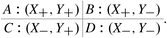
- 5.

References
Abou-Moustafa KT, De La Torre F, Ferrie FP (2010) Designing a metric for the difference between Gaussian densities. In: Angeles J, Boulet B, Clark J J, Kövecses J, Siddiqi K (eds) Brain, body and machine. Springer, Berlin, pp 57–70
Aczél J, Wagner C (1980) A characterisation of weighted arithmetic means. SIAM J Algebr Discrete Methods 1(3):259–260
Ajzen I (1977) Intuitive theories of events and the effects of base-rate information on prediction. J Pers Soc Psychol 35(5):303–314
Allan LG (1980) A note on measurement of contingency between two binary variables in judgment tasks. Bull Psychon Soc 15(3):147–149
Balakrishnan N, Nevzorov VB (2004) A primer on statistical distributions. Wiley, Hoboken
Bar-Hillel M (1980) The base-rate fallacy in probability judgments. Acta Psychol 44(3):211–233
Batanero C, Díaz C (2012) Training school teachers to teach probability: reflections and challenges. Chilean J Stat 3(1):3–13
Bechlivanidis C, Lagnado DA (2013) Does the “why” tell us the “when”? Psychol Sci 24(8):1563–1572
Bedford T, Cooke RM (2001) Probabilistic risk analysis: foundations and methods. Cambridge University Press, Cambridge
Bertsch McGrayne S (2011) The theory that would not die. Yale University Press, New Haven
Bes B, Sloman S, Lucas CG and Raufaste E (2012) Non-Bayesian inference: causal structure trumps correlation. Cogn Sci 36(7):1178–1203
Bolger F, Wright G (1994) Assessing the quality of expert judgment: issues and analysis. Decis Support Syst 11(1):1–24
Borovcnik M, Kapadia R (2014) From puzzles and paradoxes to concepts in probability. In: Chernoff EJ, Sriraman B (eds) Probabilistic thinking. Springer, Dordrecht, pp 35–73
Bradley R, Dietrich F, List C (2014) Aggregating causal judgments. Philos Sci 81(4):491–515
Browne GJ, Curley SP, Benson PG (1997) Evoking information in probability assessment: knowledge maps and reasoning-based directed questions. Manag Sci 43(1):1–14
Carranza P, Kuzniak A (2009) Duality of probability and statistics teaching in French education. In: Batanero C (ed) Joint ICMI/IASE study: teaching statistics in school mathematics, p 5
Chapman LJ, Chapman JP (1969) Illusory correlation as an obstacle to the use of valid psychodiagnostic signs. J Abnorm Psychol 74(3):271–280
Clemen RT, Reilly T (1999) Correlations and copulas for decision and risk analysis. Manag Sci 45(2):208–224
Clemen RT, Reilly T (2014) Making hard decisions with decision tools. South-Western, Mason
Clemen RT, Fischer GW, Winkler RL (2000) Assessing dependence: some experimental results. Manag Sci 46(8):1100–1115
Cooke RM (1991) Experts in uncertainty: opinion and subjective probability in Science. Oxford University Press, New York
Cooke RM (2013) Uncertainty analysis comes to integrated assessment models for climate change and conversely. Climatic Change 117(3):467–479
Cooke RM, Goossens LHJ (1999) Procedures guide for structured expert judgment. Commission of the European Communities, Brussels
Cooke RM, Goossens LHJ (2004) Expert judgement elicitation for risk assessments of critical infrastructures. J Risk Res 7(6):643–656
Cooke RM, Goossens LHJ (2008) TU Delft expert judgment data base. Reliab Eng Syst Saf 93(5):657–674
Costello FJ (2009) How probability theory explains the conjunction fallacy. J Behav Decis Mak 22(3):213–234
Dawes RM (1988) Rational choice in an uncertain world. Harcourt, Brace, Jovanovich, New York
DeGroot MH (1974) Reaching a consensus. J Am Stat Assoc 69(345):118–121
Díaz C, Batanero C, Contreras JM (2010) Teaching independence and conditional probability. Boletín de Estadística e Investigación Operativa 26(2):149–162
Dietrich F, List C (2016) Probabilistic Opinion Pooling. In: Hajek A, Hitchcock C (eds) The oxford handbook of probability and philosophy. Oxford handbooks. Oxford University Press, Oxford, pp 179–207
DuCharme WM (1970) Response bias explanation of conservative human inference. J Exp Psychol 85(1):66–74
Eddy DM (1982) Probabilistic reasoning in clinical medicine: problems and opportunities. In: Kahneman D, Slovic P and Tversky A (eds) Judgment under uncertainty: heuristics and biases. Cambridge University Press, New York, pp 249–267
Eder AB, Fiedler K, Hamm-Eder S (2011) Illusory correlations revisited: the role of pseudocontingencies and working-memory capacity. Q J Exp Psychol 64(3):517–532
Edwards W (1965) Optimal strategies for seeking information: models for statistics, choice reaction times, and human information processing. J Math Psychol 2(2):312–329
EFSA=European Food and Safety Authority (Bolger F, Hanea AM, O’Hagan A, Mosbach-Schulz O, Oakley J, Rowe G, Wenholt M) (2014) Guidance on expert knowledge elicitation in food and feed safety risk assessment. EFSA J 12(6):3734
Eichler A, Vogel M (2014) Three Approaches for Modelling Situations with Randomness. In: Chernoff EJ, Sriraman B (eds) Probabilistic thinking. Springer, Dordrecht, pp 75–99
Einhorn HJ, Hogarth RM (1986) Judging probable cause. Psychol Bull 99(1):3–19
Falk R (1983) Conditional probabilities: insights and difficulties. In: Tall D (ed) Proceedings of the third international conference for the psychology of mathematics education, Warwick, 1983
Fenton NE, Neil M (2013) Risk Assessment and Decision Analysis with Bayesian Networks. Taylor and Francis Group, Boca Raton
Fenton NE, Neil M, Caballero JG (2007) Using Ranked Nodes to Model Qualitative Judgments in Bayesian Networks. IEEE Trans Knowl Data Eng 19(10):1420–1432
Fiedler K, Brinkmann B, Betsch T, Wild B (2000) A sampling approach to biases in conditional probability judgments: beyond base rate neglect and statistical format. J Exp Psychol Gen 129(3):399–418
Flores MJ, Nicholson AE, Brunskill A, Korb KB, Mascaro S (2011) Incorporating expert knowledge when learning Bayesian network structure: a medical case study. Artif Intell Med 53(3):181–204
Fountain J, Gunby P (2011) Ambiguity, the certainty illusion, and the natural frequency approach to reasoning with inverse probabilities. N Z Econ Pap 45(1-2):195–207
French S (2011) Aggregating expert judgement. Revista de la Real Academia de Ciencias Exactas, Fisicas y Naturales. Ser A Mate 105(1):181–206
Gal I (2002) Adults’ statistical literacy: meanings, components, responsibilities. Int Stat Rev 70(1):1–25
Garthwaite PH, Kadane JB, O’Hagan A (2005) Statistical methods for eliciting probability distributions. J Am Stat Assoc 100(470):680–701
Gavanski I, Hui C (1992) Natural sample spaces and uncertain belief. J Pers Soc Psychol 63(5):766–780
Gilovich T, Griffin D, Kahneman D (2002) Heuristics and biases: the psychology of intuitive judgment. Cambridge University Press, New York
Gokhale DV, Press SJ (1982) Assessment of a prior distribution for the correlation coefficient in a bivariate normal distribution. J R Stat Soc Ser A (General) 145:237–249
Goldstein M, Wooff D (2007) Bayes linear statistics, theory and methods. Wiley, Chichester
Hamilton DL (2015) Cognitive processes in stereotyping and intergroup behavior. Psychology Press, New York
Hanea A, McBride MF, Burgman MA, Wintle BC, Fidler F, Flander L, Twardy CR, Manning B, Mascaro S (2017) Investigate discuss estimate aggregate for structured expert judgement. Int J Forecast 33:267–279
Hanea A, Morales Nápoles O, Ababei D (2015) Non-parametric Bayesian networks: improving theory and reviewing applications. Reliab Eng Syst Saf 144:265–284
Hanea D, Ale B (2009) Risk of human fatality in building fires: a decision tool using Bayesian networks. Fire Saf J 44(5):704–710
Hastie R (2016) Causal thinking in judgments. In: Keren G, Wu G (eds) The Wiley Blackwell handbook of judgment and decision making. Wiley, Chichester, pp 590–628
Hastie R, Dawes RM (2001) Rational choice in an uncertain world. Sage, Thousand Oaks
Henrion M (1989) Some practical issues in constructing belief networks. In: Kanal L, Levitt T, Lemmer J (eds) Uncertainty in artificial intelligence. Elsevier Science Publishing Company, New York, pp 132–139
Hora SC (2007) Eliciting Probabilities from Experts. In: Edwards W, Miles RF Jr, Von Winterfeldt D (eds) Advances in decision analysis - from foundations to applications. Cambridge University Press, New York, pp 129–163
Hora SC, Kardeş E (2015) Calibration, sharpness and the weighting of experts in a linear opinion pool. Ann Oper Res 229(1):429–450
Howard RA (1989) Knowledge maps. Manag Sci 35(8):903–922
Howard RA, Matheson JE (2005) Influence diagrams. Decis Anal 2(3):127–143
Hume D (1748/2000) An enquiry concerning human understanding. Beauchamp TL (ed) Oxford University Press, New York
Joe H (2014) Dependence modeling with copulas. Chapman and Hall, Boca Raton
Kadane J, Wolfson LJ (1998) Experiences in elicitation. J R Stat Soc Ser D (Stat) 47(1):3–19
Kahneman D, Frederick S (2002) Representativeness revisited: attribute substitution in intuitive judgment. In: Gilovich T, Griffin D, Kahneman D (eds) Heuristics of intuitive judgment: extensions and applications, 1st edn. Cambridge University Press, New York, pp 19–49
Kahneman D, Tversky A (1972) Subjective probability: a judgment of representativeness. Cogn Psychol 3(3):430–454
Kahneman D, Tversky A (1973) On the psychology of prediction. Psychol Rev 80(4):237–251
Kao SF, Wasserman EA (1993) Assessment of an information integration account of contingency judgment with examination of subjective cell importance and method of information presentation. J Exp Psychol Learn Mem Cogn 19(6):1363–1386
Keeney RL, Von Winterfeldt D (1991) Eliciting probabilities from experts in complex technical problems. IEEE Trans Eng Manag 38(3):191–201
Keren G, Teigen KH (2006) Yet another look at Heuristics and biases approach. In: Koehler DJ, Harvey N (eds) Blackwell handbook of judgment and decision making, 1st edn. Blackwell Publishing, Oxford, p 89–109
Kleinmuntz DN, Fennema MG, Peecher ME (1996) Conditioned assessment of subjective probabilities: Identifying the benefits of decomposition. Organ Behav Hum Decis Process 66(1):1–15
Koehler JJ (1996) The base rate fallacy reconsidered: descriptive, normative, and methodological challenges. Behav Brain Sci 19(1):1–17
Kraan BCP (2002) Probabilistic inversion in uncertainty analysis: and related topics. PhD Thesis, Delft University of Technology, The Netherlands
Kruskal WH (1958) Ordinal measures of association. J Am Stat Assoc 53(284):814–861
Kurowicka D, Cooke RM (2006) Uncertainty analysis with high dimensional dependence modelling. Wiley, Chichester
Kynn M (2008) The “heuristics and biases” bias in expert elicitation. J R Stat Soc Ser A (Stat Soc) 171(1):239–264
Lad F (1996) Operational subjective statistical methods: a mathematical, philosophical, and historical introduction. Wiley-Interscience, New York
Lagnado DA, Shanks DR (2002) Probability judgment in hierarchical learning: a conflict between predictiveness and coherence. Cognition 83(1):81–112
Lagnado DA, Sloman SA (2006) Inside and outside probability judgment. In: Koehler DJ, Harvey N (eds) Blackwell handbook of judgment and decision making, 1st edn. Blackwell Publishing, Oxford, pp 157–176
Liu TC, Lin YC (2010) The application of Simulation Assisted Learning Statistics (SALS) for correcting misconceptions and improving understanding of correlation. J Comput Assis Learn 26(2):143–158
Mandel DR, Lehman DR (1998) Integration of contingency information in judgments of cause, covariation, and probability. J Exp Psychol Gen 127(3):269–285
McConway KJ (1981) Marginalization and linear opinion pools. J Am Stat Assoc 76(374):410–414
McKenzie CR, Mikkelsen LA (2007) A Bayesian view of covariation assessment. Cogn Psychol 54(1):33–61
Meder B, Gigerenzer G (2014) Statistical thinking: no one left behind. In: Chernoff EJ, Sriraman B (eds) Probabilistic thinking. Springer, Dordrecht, pp 127–148
Medin DL, Coley JD, Storms G, Hayes BL (2003) A relevance theory of induction. Psychon Bull Rev 10(3):517–532
Meehl PE, Rosen A (1955) Antecedent probability and the efficiency of psychometric signs, patterns, and cutting scores. Psychol Bull 52:194–216
Merkhofer MW (1987) Quantifying judgmental uncertainty: Methodology, experiences, and insights. IEEE Trans Syst Man Cybern 17(5):741–752
Mitchell CJ, De Houwer J, Lovibond PF (2009) The propositional nature of human associative learning. Behav Brain Sci 32(2):183–198
Mkrtchyan L, Podofillini L, Dang VN (2015) Bayesian belief networks for human reliability analysis: a review of applications and gaps. Reliab Eng Syst Saf 139:1–16
Montibeller G, Von Winterfeldt D (2015) Cognitive and motivational biases in decision and risk analysis. Risk Anal 35(7):1230–1251
Morales-Nápoles O (2010) Bayesian belief nets and vines in aviation safety and other applications. PhD Thesis, Delft University of Technology, The Netherlands
Morales-Nápoles O, Worm DTH (2013) Hypothesis testing of Multidimensional probability distributions. WP4 GAMES2R TNO Report No. 0100003764, TNO, The Netherlands
Morales-Nápoles O, Hanea AM, Worm DTH (2013) Experimental results about the assessments of conditional rank correlations by experts: Example with air pollution estimates. In: Proceedings of the 22nd European safety and reliability conference safety, reliability and risk analysis. University of Amsterdam, Amsterdam, 2013
Morales-Nápoles O, Worm DTH, Abspoel LM, Huibregtse E, Courage W (2015) Trends and uncertainties regarding rain intensity in the Netherlands. TNO 2015 R10009, TNO
Morales-Nápoles O, Paprotny D, Worm DTH, Abspoel LM, Courage W (2016a) Characterization of precipitation through copulas and expert judgement for risk assessment of infrastructure. In: Proceedings of the 25th European safety and reliability conference safety, reliability and risk analysis. Eidgenössische Technische Hochschule Zürich, Zürich, 2016
Morales-Nápoles O, Paprotny D, Worm D, Abspoel-Bukman L, Courage W (2017) Characterization of precipitation through copulas and expert judgement for risk assessment of infrastructure. ASCE-ASME J Risk and Uncertain Eng Syst A Civ Eng 3(4), 04017012
Morgan MG, Henrion M (1990) Uncertainty: a guide to dealing with uncertainty in quantitative risk and policy analysis. Cambridge University Press, New York
Mosleh A, Apostolakis G (1986) The assessment of probability distributions from expert opinions with an application to seismic fragility curves. Risk Anal 6(4):447–461
Norrington L, Quigley J, Russell A, Van der Meer R (2008) Modelling the reliability of search and rescue operations with Bayesian belief networks. Reliab Eng Syst Saf 93(7):940–949
O’Hagan A, Buck CE, Daneshkhah A, Eiser JR, Garthwaite PH, Jenkinson DJ, Oakley JE, Rakow T (2006) Uncertain judgements: eliciting experts’ probabilities. Wiley, Chichester
Over D (2004) Rationality and the normative/descriptive distinction. In: Koehler DJ, Harvey N (eds) Blackwell handbook of judgment and decision making, 1st edn. Blackwell Publishing, Oxford, pp 3–18
Pearl J (1988) Probabilistic reasoning in intelligent systems: networks of plausible inference. Morgan Kaufmann, San Francisco
Pearl J (2009) Causality: models, reasoning, and inference. Cambridge University Press, Cambridge
Pollatsek A, Well AD, Konold C, Hardiman P, Cobb G (1987) Understanding conditional probabilities. Organ. Behav Hum Decis Process 40(2):255–269
Pollino CA, Woodberry O, Nicholson A, Korb K, Hart BT (2007) Parameterisation and evaluation of a Bayesian network for use in an ecological risk assessment. Environ Model Softw 22(8):1140–1152
Pólya G (1941) Heuristic reasoning and the theory of probability. Am Math Mon 48(7):450–465
Ramsey FP (1926) Truth and probability. In: Braithwaite RB (ed) Ramsey FP (1931) The foundations of mathematics and other logical essays. Kegan, Paul, Trench, Trubner and Co, London, pp 156–198
Revie M, Bedford T, Walls L (2010) Evaluation of elicitation methods to quantify Bayes linear models. J Risk Reliab 224(4):322–332
Rottman BM, Hastie R (2014) Reasoning about causal relationships: inferences on causal networks. Psychol Bull 140(1):109–139
Rowe G, Wright G (2001) Expert opinions in forecasting: the role of the Delphi technique. In: Armstrong JS (ed) Principles of forecasting. Springer, New York, pp 125–144
Russell B (1912) On the notion of cause. Proc Aristot Soc 13:1–26
Shachter RD (1988) Probabilistic inference and influence diagrams. Oper Res 36(4):589–604
Simon HA (1957) Models of man: social and rational. Wiley, New York
Sklar M (1959) Fonctions de répartitionà n dimensions et leurs marges. Publ Inst Statist Univ Paris 8:229–231
Sloman SA, Lagnado D (2005) The problem of induction. In: Holyoak KJ, Morrison RG (eds) The Cambridge handbook of thinking and reasoning. Cambridge University Press, New York, pp 95–116
Smedslund J (1963) The concept of correlation in adults. Scand J Psychol 4(1):165–173
Spetzler CS, Staël von Holstein CA (1975) Exceptional paper-probability encoding in decision analysis. Manag Sci 22(3):340–358
Spirtes P, Glymour CN, Scheines R (2000) Causation, prediction, and search. MIT Press, Cambridge
Staël von Holstein CA, Matheson JE (1979) A manual for encoding probability distributions. In: Defense advanced research projects agency, decisions and designs. SRI International, Menlo Park, CA
Stanovich KE, West RF (2000) Individual differences in reasoning: implications for the rationality debate? Behav Brain Sci 23:645–726
Stone M (1961) The opinion pool. Ann Math Stat 32(4):1339–1342
Suppes P (1970) A probabilistic theory of causality. North-Holland Publishing, Amsterdam
Swain AD, Guttman HE (1983) Handbook of human reliability analysis with emphasis on nuclear power plant applications. US Nuclear Regulatory Commission. NUREG/CR-1278, Washington, DC
Tentori K, Crupi V, Russo S (2013) On the determinants of the conjunction fallacy: probability versus inductive confirmation. J Exp Psychol Gen 142(1):235–255
Tversky A, Kahneman D (1973) Availability: a heuristic for judging frequency and probability. Cogn Psychol 5(2):207–232
Tversky A, Kahneman D (1980) Causal schemas in judgments under uncertainty. Progress Soc Psychol 1:49–72
Tversky A, Kahneman D (1983) Extensional versus intuitive reasoning: the conjunction fallacy in probability judgment. Psychol Rev 90(4):293–315
USNRC = US Nuclear Regulatory Commission (1975) Reactor safety study: An assessment of accident risks in U.S. commercial nuclear power plants. NUREG 75–014, Washington, DC
USNRC = US Nuclear Regulatory Commission (1987) Reactor risk reference document. NUREG-1150, Washington, DC
Utts J (2003) What educated citizens should know about statistics and probability. Am Stat 57(2):74–79
Villejoubert G, Mandel DR (2002) The inverse fallacy: an account of deviations from Bayes’s theorem and the additivity principle. Mem Cogn 30(2):171–178
Walls L, Quigley J (2001) Building prior distributions to support Bayesian reliability growth modelling using expert judgement. Reliab Eng Syst Saf 74(2):117–128
Werner C, Bedford T, Cooke RM, Hanea AM, Morales Nápoles, O (2017) Expert judgement for dependence in probabilistic modelling: a systematic literature review and future research directions. Eur J Oper Res 258(3):801–819
Wilson KJ (2017) An investigation of dependence in expert judgement studies with multiple experts. Int J Forecast 33(1):325–336
Winkler RL, Clemen RT (2004) Multiple experts vs. multiple methods: combining correlation assessments. Decis Anal 1(3):167–176
Wright G, Goodwin P (2009) Decision making and planning under low levels of predictability: Enhancing the scenario method. Int J Forecast 25(4):813–825
Wunderlich K, Symmonds M, Bossaerts P, Dolan RJ (2011) Hedging your bets by learning reward correlations in the human brain. Neuron 71(6):1141–1152
Zwirglmaier K, Straub D (2016) Approaches to Bayesian network structure elicitation. In: Walls L, Revie M, Bedford T (eds) Risk, reliability and safety: innovating theory and practice. Proceedings of the 26th European safety and reliability conference, ESREL 2016, Glasgow, September 2016. Taylor and Francis Group, London, p 333
Acknowledgements
We would like to thank the editors for the feedback on the previous version of this chapter.
Author information
Authors and Affiliations
Corresponding author
Editor information
Editors and Affiliations
Rights and permissions
Copyright information
© 2018 Springer International Publishing AG
About this chapter

Cite this chapter
Werner, C., Hanea, A.M., Morales-Nápoles, O. (2018). Eliciting Multivariate Uncertainty from Experts: Considerations and Approaches Along the Expert Judgement Process. In: Dias, L., Morton, A., Quigley, J. (eds) Elicitation. International Series in Operations Research & Management Science, vol 261. Springer, Cham. https://doi.org/10.1007/978-3-319-65052-4_8
Download citation
DOI: https://doi.org/10.1007/978-3-319-65052-4_8
Published:
Publisher Name: Springer, Cham
Print ISBN: 978-3-319-65051-7
Online ISBN: 978-3-319-65052-4
eBook Packages: Business and ManagementBusiness and Management (R0)