
Abstract
Scheduling jobs on unrelated machines and minimizing the makespan is a classical problem in combinatorial optimization. A job j has a processing time \(p_{ij}\) for every machine i. The best polynomial algorithm known for this problem goes back to Lenstra et al. and has an approximation ratio of 2. In this paper we study the Restricted Assignment problem, which is the special case where \(p_{ij}\in \{p_j,\infty \}\). We present an algorithm for this problem with an approximation ratio of \(11/6 + \epsilon \) and quasi-polynomial running time \(n^{\mathcal O(1/\epsilon \log (n))}\) for every \(\epsilon > 0\). This closes the gap to the best estimation algorithm known for the problem with regard to quasi-polynomial running time.
Research supported by German Research Foundation (DFG) project JA 612/15-1.
Access provided by CONRICYT-eBooks. Download conference paper PDF
Keywords
1 Introduction
In the problem we consider, which is known as Scheduling on Unrelated Machines, a schedule \(\sigma : \mathcal J\rightarrow \mathcal M\) of the jobs \(\mathcal J\) to the machines \(\mathcal M\) has to be computed. On machine i the job j has a processing time of \(p_{ij}\). We want to minimize the makespan, i.e., \(\max _{i\in \mathcal M}\sum _{j\in \sigma ^{-1}(i)} p_{ij}\). The classical 2-approximation by Lenstra et al. [8] is still the algorithm of choice for this problem.
Recently a special case, namely the Restricted Assignment problem, has drawn much attention in the scientific community. Here each job j has a processing time \(p_j\), which is independent from the machines, and a set of machines \(\varGamma (j)\). A job j can only be assigned to \(\varGamma (j)\). This is equivalent to the former problem when \(p_{ij}\in \{p_j,\infty \}\). For both the general and the restricted variant there cannot be a polynomial algorithm with an approximation ratio better than 3/2, unless \(\mathrm {P}=\mathrm {NP}\) [8]. If the exponential time hypothesis (ETH) holds, such an algorithm does not even exist with sub-exponential (in particular, quasi-polynomial) running time [5].
In a recent breakthrough, Svensson has proved that the configuration-LP, a natural linear programming relaxation, has an integrality gap of at most 33/17 [10]. We have later improved this bound to 11/6 [7]. By approximating the configuration-LP this yields an \((11/6 + \epsilon )\)-estimation algorithm. However, no polynomial algorithm is known that can produce a solution of this value.
For instances with only two processing times additional progress has been made. Chakrabarty et al. gave a polynomial \((2-\delta )\)-approximation for a very small \(\delta \) [4]. Later Annamalai surpassed this with a \((17/9 + \epsilon )\)-approximation for every \(\epsilon > 0\) [1]. For this special case it was also shown that the integrality gap is at most 5/3 [6].
In [6, 7, 10] the critical idea is to design a local search algorithm, which is then shown to produce good solutions. However, the algorithm has a potentially high running time; so it was only used to prove the existence of such a solution. A similar algorithm was used in the Restricted Max-Min Fair Allocation problem. Here a quasi-polynomial variant by Polácek et al. [9] and a polynomial variant by Annamalai et al. [2] were later discovered.
In this paper, we present a variant of the local search algorithm, that admits a quasi-polynomial running time. The algorithm is purely combinatorial and uses the configuration-LP only in the analysis.
Theorem 1
For every \(\epsilon > 0\) there is an \((11/6 + \epsilon )\)-approximation algorithm for the Restricted Assignment problem with running time \(\exp (\mathcal O(1/\epsilon \cdot \log ^2(n)))\), where \(n = |\mathcal {J}| + |\mathcal {M}|\).
The main idea is the concept of layers. The central data structure in the local search algorithm is a tree of so-called blockers and we partition this tree into layers, that are closely related to the distance of a blocker from the root. Roughly speaking, we prevent the tree from growing arbitrarily high. A similar approach was taken in [9].
1.1 The Configuration-LP
A well known relaxation for the problem of Scheduling on Unrelated Machines is the configuration-LP (see Fig. 1). The set of configurations with respect to a makespan T are defined as \(\mathcal C_i(T) = \{C\subseteq \mathcal J: \sum _{j\in C} p_{ij} \le T\}\). We refer to the minimal T for which this LP is feasible as the optimum or \(\mathrm {OPT}^*\). In the Restricted Assignment problem a job j can only be used in configurations of machines in \(\varGamma (j)\) given T is finite. We can find a solution for the LP with a value of at most \((1 + \epsilon ) \mathrm {OPT}^*\) in polynomial time for every \(\epsilon > 0\) [3].

Primal (left) and dual (right) of the configuration-LP w.r.t. makespan T
1.2 Preliminaries
In this section we simplify the problem we need to solve. The approximation ratio we will aim for is \(1 + R\), where \(R = 5/6 + 2\epsilon \). We assume that \(\epsilon < 1/12\) for our algorithm, since otherwise the 2-approximation in [8] can be used.
We will use a binary search to obtain a guess T for the value of \(\mathrm {OPT}^*\). In each iteration, our algorithm either returns a schedule with makespan at most \((1 + R) T\) or proves that T is smaller than \(\mathrm {OPT}^*\). After polynomially many iterations, we will have a solution with makespan at most \((1 + R) \mathrm {OPT}^*\). To shorten notation, we scale each size by 1/T within an iteration, that is to say our algorithm has to find a schedule of makespan \(1 + R\) or show that \(\mathrm {OPT}^* > 1\). Unless otherwise stated we will assume that \(T = 1\) when speaking about configurations or feasibility of the configuration-LP.
Definition 1 (Small, big, medium, huge jobs)
A job j is small if \(p_j \le 1/2\) and big otherwise; A big job is medium if \(p_j \le 5/6\) and huge if \(p_j > 5/6\).
The sets of small (big, medium, huge) jobs are denoted by \(\mathcal {J}_S\) (respectively, \(\mathcal {J}_B\), \(\mathcal {J}_M\), \(\mathcal {J}_H\)). Note that at most one big job can be in a configuration (w.r.t. makespan 1).
Definition 2 (Valid partial schedule)
We call \(\sigma : \mathcal {J}\rightarrow \mathcal {M}\cup \{\bot \}\) a valid partial schedule if (1) for each job j we have \(\sigma (j)\in \varGamma (j)\cup \{\bot \}\), (2) for each machine \(i\in \mathcal {M}\) we have \(p(\sigma ^{-1}(i)) \le 1 + R\), and (3) each machine is assigned at most one huge job.
\(\sigma (j) = \bot \) means that job j has not been assigned. In each iteration of the binary search, we will first find a valid partial schedule for all medium and small jobs and then extend the schedule one huge job at a time. We can find a schedule for all small and medium jobs with makespan at most 11/6 by applying the algorithm by Lenstra, Shmoys, and Tardos [8]. This algorithm outputs a solution with makespan at most \(\mathrm {OPT}^* + p_{max}\), where \(p_{max}\) is the biggest processing time (in our case at most 5/6). The problem that remains to be solved is given in below.

Without loss of generality let us assume that the jobs are identified by natural numbers, that is \(\mathcal {J}= \{1,2,\cdots , |\mathcal {J}|\}\), and \(p_1 \le p_2 \le \cdots \le p_{|\mathcal {J}|}\). This gives us a total order on the jobs that will simplify the algorithm.
2 Algorithm
Throughout the paper, we make use of modified processing times \(\overline{P}_j\) and \(\overline{p}_j\), which we obtain by rounding the sizes of huge jobs up or down, that is
Definition 3 (Moves, valid moves)
A pair \((j,\, i)\) of a job j and a machine i is a move, if \(i\in \varGamma (j)\backslash \{\sigma (j)\}\). A move (j, i) is valid, if (1) \(\overline{P}(\sigma ^{-1}(i)) + p_j \le 1 + R\) and (2) j is not huge or no huge job is already on i.
We note that by performing a valid move (j, i) the properties of a valid partial schedule are not compromised.
Definition 4 (Blockers)
A blocker is a tuple \((j, i, \varTheta )\), where (j, i) is a move and \(\varTheta \) is the type of the blocker. There are 6 types with the following abbreviations: (SA) small-to-any blockers, (HA) huge-to-any blockers, (MA) medium-to-any blockers, (BH) huge-/medium-to-huge blockers, (HM) huge-to-medium blockers, and (HL) huge-to-least blockers.
The algorithm maintains a set of blockers called the blocker tree  . We will discuss the tree analogy later. The blockers wrap moves that the algorithm would like to execute. By abuse of notation, we write that a move (j, i) is in
  , if there is a blocker \((j, i, \varTheta )\) in
  for some \(\varTheta \). The type \(\varTheta \) determines how the algorithm treats the machine i as we will elaborate below.
The first part of a type’s name refers to the size of the blocker’s job, e.g., small-to-any blockers are only used with small jobs, huge-to-any blockers only with huge jobs, etc. The latter part of the type’s name describes the undesirable jobs on the machine: The algorithm will try to remove jobs from this machine if they are undesirable; at the same time it does not attempt to add such jobs to the machine. On machines of small-/medium-/huge-to-any blockers all jobs are undesirable; on machines of huge-/medium-to-huge blockers huge jobs are undesirable; on machines of huge-to-medium blockers medium jobs are undesirable and finally on machines of huge-to-least blockers only those medium jobs of index smaller or equal to the smallest medium job on i are undesirable.
The same machine can appear more than once in the blocker tree. In that case, the undesirable jobs are the union of the undesirable jobs from all types. Also, the same job can appear multiple times in different blockers.
The blockers corresponding to specific types are written as  ,
,  , etc. From the blocker tree, we derive the machine set
  which consists of all machines corresponding to moves in
  . This notation is also used with subsets of
  , e.g.,
  .
.
Definition 5 (Blocked small jobs, active jobs)
A small job j is blocked, if it is undesirable on all other machines it allowed on, that is  . We denote the set of blocked small jobs by
  . The set of active jobs \(\mathcal A\) includes \(j_\mathrm {new}\),
  as well as all those jobs, that are undesirable on the machine, they are currently assigned to.
We define for all machines i the job sets  ,
,  , \(M_i = \sigma ^{-1}(i) \cap \mathcal {J}_M\) and \(H_i = \sigma ^{-1}(i) \cap \mathcal {J}_H\). Moreover, set \(M^{\min }_{i} = \{\min M_i\}\) if \(M_i\ne \emptyset \) and \(M^{\min }_{i} = \emptyset \) otherwise.
2.1 Tree and Layers
The blockers in  and an additional root can be imagined as a tree. The parent of each blocker \(\mathcal {B}_{} = (j, i, \varTheta )\) is only determined by j. If \(j = j_\mathrm {new}\) it is the root node; otherwise it is a blocker
  for machine \(\sigma (j)\) with a type for which j is regarded undesirable. If this applies to several blockers, we use the one that was added to the blocker tree first. We say that \(\mathcal {B}_{}'\) activates j.
Let us now introduce the notion of a layer. Each blocker is assigned to exactly one layer. The layer roughly correlates with the distance of the blocker to the root node. In this sense, the children of a blocker are usually in the next layer. There are some exceptions, however, in which a child is in the same layer as its parent. We now define the layer of the children of a blocker \(\mathcal {B}_{}\) in layer k.
-
1.
If \(\mathcal {B}_{}\) is a huge-/medium-to-huge blocker, all its children are in layer k as well;
-
2.
if \(\mathcal {B}_{}\) is a huge-to-any blocker, children regarding small jobs are in layer k as well;
-
3.
in every other case, the children are in layer \(k + 1\).
We note that by this definition for an active job j all blockers  must be in the same layer; in other words, it is unambiguous in which layer blockers for it would be placed in. We say j is k
-headed, if blockers for j would be placed in layer k. The blockers in layer k are denoted by
must be in the same layer; in other words, it is unambiguous in which layer blockers for it would be placed in. We say j is k
-headed, if blockers for j would be placed in layer k. The blockers in layer k are denoted by  . The set of blockers in layer k and below is referred to by
  . We use this notation in combination with qualifiers for the type of blocker, e.g.,
  .
.
We establish an order between the types of blockers within a layer and refer to this order as the sublayer number. The huge-/medium-to-huge blockers form the first sublayer of each layer, huge-to-any and medium-to-any blockers the second, small-to-any blockers the third, huge-to-least the fourth and huge-to-medium blockers the fifth sublayer (see also Table 1 and Fig. 2). By saying a sublayer is after (before) another sublayer we mean that either its layer is higher (lower) or both layers are the same and its sublayer number is higher (lower).

Example layer

In the final algorithm whenever we remove one blocker, we also remove all blockers in its sublayer and all later sublayers (in particular, all descendants). Also, when we add a blocker to a sublayer, we remove all later sublayers. Among other properties, this guarantees that the connectivity of the tree is never compromised. It also means that, if j is undesirable regarding several blockers for \(\sigma (j)\), then the parent is in the lowest sublayer among these blockers, since a blocker in a lower sublayer cannot have been added after one in a higher sublayer.
The running time will be exponential in the number of layers; hence this should be fairly small. We introduce an upper bound \(K = 2/\epsilon \lceil \ln (|\mathcal {M}|) + 1 \rceil = \mathcal O(1/\epsilon \cdot \log (|\mathcal {M}|))\) and will not add any blockers to a layer higher than K.
2.2 Detailed Description of the Algorithm
The algorithm (see Algorithm 1) contains a loop that terminates once \(j_\mathrm {new}\) is assigned. In each iteration the algorithm performs a valid move in the blocker tree if possible and otherwise adds a new blocker.
Adding blockers. We only add a move to  , if it meets certain requirements. A move that does is called a potential move. For each type of blocker we also define a type of potential move: Potential small-to-any moves, potential huge-to-any moves, etc. When a potential move is added to the blocker tree, its type will then be used for the blocker. Let k be a layer and let
  be k-headed. For a move (j, i) to be a potential move of a certain type, it has to meet the following requirements.
-
1.
(j, i) is not already in
 ;
; -
2.
the size of j corresponds to the type, for instance, if j is big, (j, i) cannot be a small-to-any move;
-
3.
j is not undesirable on i w.r.t.
 , i.e., (a)
  and (b) if j is huge, then
  ; (c) if j is medium, then
  and either
  or \(\min M_i < j\).
 -
4.
The load of the target machine has to meet certain conditions (see Table 1).
 ;
; , i.e., (a)
  and (b) if j is huge, then
  ; (c) if j is medium, then
  and either
  or
or Comparing the conditions in the table we notice that for moves of small and medium jobs there is always exactly one type that applies. For huge jobs there is exactly one type if  and no type applies, if
  . The table also lists a priority for each type of move. It is worth mentioning that the priority does not directly correlate with the sublayer. The algorithm will choose the move that can be added to the lowest layer and among those has the highest priority. After adding a blocker, all higher sublayers are deleted.
Performing valid moves. The algorithm performs a valid move in  if there is one. It chooses a blocker \((j,i,\varTheta )\) in
  , where the blocker’s sublayer is minimal and (j, i) is valid. Besides assigning j to i,
  has to be updated as well.
Let \(\mathcal {B}_{}\) be the blocker that activated j. When certain conditions for \(\mathcal {B}_{}\) are no longer met, we will delete \(\mathcal {B}_{}\) and its sublayer. The conditions that need to be checked depend on the type of \(\mathcal {B}_{}\) and are marked in Table 1 with a star (\(*\)). In any case, the algorithm will discards all blockers in higher sublayers than \(\mathcal {B}_{}\) is.
3 Analysis
The analysis of the algorithm has two critical parts. First, we show that it does not get stuck, i.e., there is always a blocker that can be added to the blocker tree or a move that can be executed. Then we show that the number of iterations is bounded by \(\exp (\mathcal O(1/\epsilon \log ^2(n)))\).
Theorem 2
If the algorithm returns ‘error’, then \(\mathrm {OPT}^* > 1\).
The proof consists in the construction of a solution \((z^*, y^*)\) for the dual of the configuration-LP. The value \(z^*_j\) is composed of \(\overline{p}_j\) and a scaling coefficient (a power of \(\delta := 1 - \epsilon \)). The idea of the scaling coefficient is that values for jobs activated in higher layers are supposed to get smaller and smaller. We set \(z^*_j = 0\) if  and \(z^*_j = \delta ^k \cdot \overline{p}_j\), if
  and k is the smallest layer such that j is k-headed or
  . For all \(i\in \mathcal {M}\) let

Finally set \(y^*_i = \delta ^K + w_i\). Note that w is well-defined, since a machine i can be in at most one of the sets  On a small-/huge-to-any blocker all jobs are undesirable, that is to say as long as one of such blockers remains in the blocker tree, the algorithm will not add another blocker with the same machine. Also note that
  and \(z^*(\sigma ^{-1}(i))\) are interchangeable.
Lemma 1
If there is no valid move in  and no potential move of a k-headed job for a \(k\le K\), the value of the solution is negative, i.e., \(\sum _{j\in \mathcal J} z^*_j > \sum _{i\in \mathcal M} y^*_i\).
Proof
Using the Taylor series and \(\epsilon < 1/12\) it is easy to check \(\ln (1 - \epsilon ) \ge -\epsilon /2\). This gives
Claim 1
(Proof is omitted to conserve space). For all \(k \le K\) we have  .
.
Using this claim we find that

\(\square \)
Lemma 2
If there is no valid move in  and no potential move of a k-headed job for a \(k\le K\), the solution is feasible, i.e., \(z^*(C) \le y^*_i\) for all \(i\in \mathcal M\), \(C\in \mathcal C_i\).
Proof
We will make the following assumptions, that can be shown with an exhaustive case analysis.
Claim 2
(Proof is omitted to conserve space). Let \(k \le K\),  , \(C\in \mathcal C_i\), \(j\in C\) k-headed and big with \(\sigma (j)\ne i\). Then
  .
.
Claim 3
(Proof is omitted to conserve space). Let \(k\le K\) and  . Then

Let \(C_0\in \mathcal C_i\) and \(C \subseteq C_0\) denote the set of jobs j with \(z^*_j \ge \delta ^{K}\overline{p}_j\). In particular, C does not contain jobs that have potential moves. It is sufficient to show that \(z^*(C) \le w_i\), as this would imply

Loosely speaking, the purpose of \(\delta ^K\) in the definition of \(y^*\) is to compensate for ignoring all \((K+1)\)-headed jobs.
First, consider the case where  . There cannot be a small and activated job \(j_S\in C\) with \(\sigma (j_S) \ne i\), because then \((j_S, i)\) would be a potential move; hence
  . If there is a big job \(j_B\in C\) with \(\sigma (j_B) \ne i\), then

If there is no such job, then  and in particular \(z^*(C) \le w_i\).
In the remainder of this proof we assume that  . Note that for any \(k\ne \ell +1\) we have
  . Also, since all jobs on i are active we have that \(z^*_j \ge \delta ^{\ell +2} \overline{p}_j\) for all \(j\in \sigma ^{-1}(i)\). Because there is no potential move \((j_S, i)\) for a small job \(j_S\) with \(z^*_{j_S} \ge \delta ^{\ell } \overline{p}_{j_S}\), we have for all small jobs
  : \(z^*_{j_S} \le \delta ^{\ell + 1} \overline{p}_{j_S}\).
- Case 1.:
-
For every big job \({j\in C}\) with \(\sigma (j) \ne i\) we have \(z^*_j \le \delta ^{\ell + 1} \overline{p}_j\).
This implies

Therefore

- Case 2.:
-
There is a big job \(j\in C\) with \(\sigma (j) \ne i\) and \(z^*_j \ge \delta ^\ell \overline{p}_j\).
Let \(k\le \ell \) with \(z^*_j = \delta ^k \overline{p}_j\), that is to say j is k-headed. Then
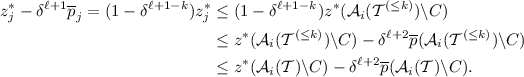
In the second inequality we use that for every
 we have \(z^*_{j'} \ge \delta ^{k+1}\cdot \overline{p}_{j'}\). This implies that
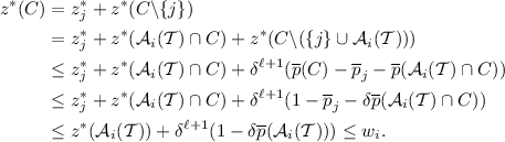


 we have
\(\square \)
We can now complete the proof of Theorem 2.
Proof
(Theorem 2 ). Suppose toward contradiction there is no potential move of a k-headed job, where \(k \le K\), and no move in the blocker tree is valid. It is obvious that since Lemmas 1 and 2 hold for \((y^*, z^*)\), they also hold for a scaled solution \((\alpha \cdot y^*, \alpha \cdot z^*)\) with \(\alpha > 0\). We can use this to obtain a solution with an arbitrarily low objective value; thereby proving that the dual is unbounded regarding makespan 1 and therefore \(\mathrm {OPT}^* > 1\). \(\square \)
Theorem 3
The algorithm terminates in time \(\exp (\mathcal O(1/\epsilon \cdot \log ^2(n)))\).
Proof
Let \(\ell \le K\) be the index of the last non-empty layer in  . We will define the so-called signature vector as
  , where \(s_k\) is given by

Each component in \(s_k\) represents a sublayer within layer k and it is the sum over certain values associated with its blockers. Note that these values are all strictly positive, since \(j_\mathrm {new}\) is not assigned and therefore \(|\sigma ^{-1}(i)| < |\mathcal {J}|\).
Claim 4
(Proof is omitted to conserve space). The signature vector increases lexicographically after polynomially many iterations of the loop.
This means that the number of possible vectors is an upper bound on the running time (except for a polynomial factor). Each sublayer has at most \(|\mathcal {J}|\cdot |\mathcal {M}|\) many blockers (since there are at most this many moves) and the value for every blocker in each of the five cases is easily bounded by \(\mathcal O(|\mathcal {J}|)\). This implies there are at most \((\mathcal O(n^3))^5 = n^{\mathcal O(1)}\) values for each \(s_k\). Using \(K = \mathcal O(1/\epsilon \log (n))\) we bound the number of different signature vectors by \(n^{\mathcal O(K)} = \exp (\mathcal O(1/\epsilon \log ^2(n)))\). \(\square \)
4 Conclusion
We have greatly improved the running time of the local search algorithm for the Restricted Assignment problem. At the same time we were able to maintain almost the same approximation ratio. We think there are two important directions for future research. The first is to improve the approximation ratio further. For this purpose, it makes sense to first find improvements for the much simpler variant of the algorithm given in [7].
The perhaps most important open question, however, is whether the running time can be brought down to a polynomial one. Recent developments in the Restricted Max-Min Fair Allocation problem indicate that a layer structure similar to the one in this paper may also help in that regard [2]. In the mentioned paper moves are only performed in large groups. This concept is referred to as laziness. The asymptotic behavior of the partition function (the number of integer partitions of a natural number) is then used in the analysis for a better bound on the number of possible signature vectors. This approach appears to have a great potential for the Restricted Assignment problem as well. In [1] it was already adapted to the special case of two processing times.
References
Annamalai, C.: Lazy local search meets machine scheduling. CoRR abs/1611.07371 (2016). http://arxiv.org/abs/1611.07371
Annamalai, C., Kalaitzis, C., Svensson, O.: Combinatorial algorithm for restricted max-min fair allocation. In: Proceedings of the Twenty-Sixth Annual ACM-SIAM Symposium on Discrete Algorithms, SODA 2015, San Diego, CA, USA, 4–6 January 2015, pp. 1357–1372 (2015). doi:10.1137/1.9781611973730.90
Bansal, N., Sviridenko, M.: The santa claus problem. In: Proceedings of the 38th Annual ACM Symposium on Theory of Computing, Seattle, WA, USA, 21–23 May 2006, pp. 31–40 (2006). doi:10.1145/1132516.1132522
Chakrabarty, D., Khanna, S., Li, S.: On \((1, \epsilon )\)-restricted assignment makespan minimization. In: Proceedings of the Twenty-Sixth Annual ACM-SIAM Symposium on Discrete Algorithms, SODA 2015, San Diego, CA, USA, 4–6 January 2015, pp. 1087–1101 (2015). doi:10.1137/1.9781611973730.73
Jansen, K., Land, F., Land, K.: Bounding the running time of algorithms for scheduling and packing problems. SIAM J. Discrete Math. 30(1), 343–366 (2016). doi:10.1137/140952636
Jansen, K., Land, K., Maack, M.: Estimating the makespan of the two-valued restricted assignment problem. In: Proceedings of the 15th Scandinavian Symposium and Workshops on Algorithm Theory, SWAT 2016, Reykjavik, Iceland, 22–24 June 2016, pp. 24:1–24:13 (2016). doi:10.4230/LIPIcs.SWAT.2016.24
Jansen, K., Rohwedder, L.: On the Configuration-LP of the restricted assignment problem. In: Proceedings of the Twenty-Eighth Annual ACM-SIAM Symposium on Discrete Algorithms, SODA 2017, Barcelona, Spain, Hotel Porta Fira, 16–19 January, pp. 2670–2678 (2017). doi:10.1137/1.9781611974782.176
Lenstra, J.K., Shmoys, D.B., Tardos, E.: Approximation algorithms for scheduling unrelated parallel machines. Math. Program. 46(3), 259–271 (1990). doi:10.1007/BF01585745
Polácek, L., Svensson, O.: Quasi-polynomial local search for restricted max-min fair allocation. ACM Trans. Algorithms 12(2), 13 (2016). doi:10.1145/2818695
Svensson, O.: Santa claus schedules jobs on unrelated machines. SIAM J. Comput. 41(5), 1318–1341 (2012). doi:10.1137/110851201
Author information
Authors and Affiliations
Corresponding author
Editor information
Editors and Affiliations
Rights and permissions
Copyright information
© 2017 Springer International Publishing AG
About this paper
Cite this paper
Jansen, K., Rohwedder, L. (2017). A Quasi-Polynomial Approximation for the Restricted Assignment Problem. In: Eisenbrand, F., Koenemann, J. (eds) Integer Programming and Combinatorial Optimization. IPCO 2017. Lecture Notes in Computer Science(), vol 10328. Springer, Cham. https://doi.org/10.1007/978-3-319-59250-3_25
Download citation
DOI: https://doi.org/10.1007/978-3-319-59250-3_25
Published:
Publisher Name: Springer, Cham
Print ISBN: 978-3-319-59249-7
Online ISBN: 978-3-319-59250-3
eBook Packages: Computer ScienceComputer Science (R0)