Components as Location Graphs

Abstract

This paper presents a process calculus framework for modeling ubiquitous computing systems and dynamic component-based structures as location graphs. A key aspect of the framework is its ability to model nested locations with sharing, while allowing the dynamic reconfiguration of the location graph, and the dynamic update of located processes.

These keywords were added by machine and not by the authors. This process is experimental and the keywords may be updated as the learning algorithm improves.

1 Introduction

Motivations. Computing systems are increasingly built as distributed, dynamic assemblages of hardware and software components. Modelling these assemblages requires capturing different kinds of dependencies and containment relationships between components. The software engineering literature is rife with analyses of different forms of whole-part, aggregation or composition relationships, and of their attendants characteristics such as emergent property, overlapping lifetimes, and existential dependency [2]. These analyses explicitly consider the possibility for a component to be shared at once between different wholes, an important requirement in particular if one expects to deal with multiple architectural views of a system.

Consider, for instance, a software system featuring a database $DB$ and a client of the database $C$. The database comprises the following (sub)components: a cache $CC$, a data store $DS$ and a query engine $QE$. Both data store and query engine reside in the same virtual machine $V_0$, for performance reasons. Client and cache reside in another virtual machine $V_1$, also for performance reasons. We have here a description which combines two architectural views, in the sense of [17]: a logical view, that identifies two high-level components, the database $DB$ and its client $C$, and the sub-components $CC, QE$ and $DS$ of the database, and a process view, that maps the above components on virtual machines $V_0$ and $V_1$. We also have two distinct containment or whole-part relationships: being placed in a virtual machine, and being part of the $DB$ database. A virtual machine is clearly a container: it represents a set of resources dedicated to the execution of the components it contains, and it manifests a failure dependency for all the components it executes (should a virtual machine fail, the components it contains also fail). The database $DB$ is clearly a composite: it represents the result of the composition of its parts (cache, query engine, and data store) together with their attendant connections and interaction protocols; it encapsulates the behavior of its subcomponents; and its lifetime constrains those of its parts (e.g. if the database is destroyed so are its subcomponents). The cache component $CC$ in this example is thus part of two wholes, the database $DB$ and the virtual machine $V_1$.

Surprisingly, most formal models of computation and software architecture do not provide support for a direct modelling of containment structures with sharing. On the one hand, one finds numerous formal models of computation and of component software with strictly hierarchic structures, such as Mobile Ambients and their different variants [6, 7], the Kell calculus [25], BIP [4], Ptolemy [26], or, at more abstract level, Milner’s bigraphs [20]. In bigraphs, for instance, it would be natural to model the containment relationships in our database example as instances of sub-node relationships in bigraphs, because nodes correspond to agents in a bigraph. Yet this is not possible because the sub-node relation in a bigraph is restricted to form a forest. To model the above example as a bigraph would require choosing which containment relation (placement in a virtual machine or being a subcomponent of the database) to represent by means of the sub-node relation, and to model the other relation by means of bigraph edges. This asymmetry in modelling is hard to justify for both containment relations are proper examples of whole-part relationships.

On the other hand, one finds formal component models such as Reo [1], $\pi$-ADL [22], Synchronized Hyperedge Replacement (SHR) systems [14], SRMLight [15], that represent only interaction structures among components, and not containment relationships, and models that support the modeling of non-hierarchical containment structures, but with other limitations. Our own work on the Kell calculus with sharing [16] allows to model non-hierarchical containment structures but places constraints on the dependencies that can be modelled. For instance, the lifetime dependency constraints associated with the virtual machines and the database in our example above (if the aggregate or composite dies so do its sub-components) cannot be both easily modeled. The reason is that the calculus still enforces an ownership tree between components for the purpose of passivation: components can only passivate components lower down in the tree (i.e. suspend their execution and capture their state). The formal model which comes closer to supporting non strictly hierarchical containment structures is probably CommUnity [28], where component containment is modelled as a form of superposition, and can be organized as an arbitrary graph. However, in CommUnity, possible reconfigurations in a component assemblage are described as graph transformation rules that are separate from the behavior of components, making it difficult to model reconfigurations initiated by the component assemblage itself.

To sum up, we are missing a model of computation that allows us to directly model both different forms of interactions and different forms of containment relationships between components; that supports both planned (i.e. built in component behaviors) and unplanned (i.e. induced by the environment) dynamic changes to these relationships, as well as to component behaviors.

Contribution. In this paper, we introduce a model of computation, called G-Kells, which meets these requirements. We develop our model at a more concrete level than bigraph theory, but we abstract from linguistic details by developing a process calculus framework parameterized by a notion of process and certain semantical operations. Computation in our model is carried out by located processes, i.e. processes that execute at named locations. Locations can be nested inside one another, and a given location can be nested inside one or more locations at once. Locations constitute scopes for interactions: a set of processes can interact when situated in locations nested within the same location. Behaviors of located processes encompass interaction with other processes as well as reconfiguration actions which may change the structure of the location graph and update located processes. In addition, the G-Kells framework supports a notion of dynamic priority that few other component models support, apart from those targeting real-time and reactive systems such as BIP and Ptolemy.

Outline. The paper is organized as follows. The framework we introduce can be understood as an outgrowth of our prior work with C. Di Giusto [13], in which we proposed a process calculus interpretation of the BIP model. We recall briefly in Sect. 2 the main elements of this work, to help explain the extensions we introduce in our G-Kells framework. Section 3 presents the G-Kells framework and its formal operational semantics. Section 4 discusses the various features of the G-Kells framework, and related work. Section 5 concludes the paper.

2 CAB: A Process Calculus Interpretation of BIP

One way to understand the G-Kells model we introduce in the next section, is to see it as a higher-order, dynamic extension of the CAB model [13], a process calculus interpretation of the BIP model. We recall briefly in this section the main elements of CAB.

The CAB model captures the key features of the BIP model: (i) hierarchical components; (ii) composition of components via explicit “glues” enforcing multiway synchronization constraints between sub-components; (iii) priority constraints regulating interactions among components. Just as the BIP model, the CAB model is parameterized by a family $\mathcal {P}$ of primitive behaviors. A CAB component, named $l$, can be either a primitive component $C = l[P]$, where $P$ is taken from $\mathcal {P}$, or a composite component $C = l[C_1, \ldots , C_n \star G]$, built by composing a set of CAB components with a glue process $G$. When $l$ is the name of a component $C$, we write . We note $\mathcal {C}$ the set of CAB components, ${\mathcal {N}_l}$ the set of location names, and ${\mathcal {N}_c}$ the set of channel names. Behaviors in $\mathcal {P}$ are defined as labelled transition systems, with labels in ${\mathcal {N}_c}$.

In CAB, the language for glues $G$ is a very simple language featuring:

• Action prefix $\xi .G$, where $\xi$ is an action, and $G$ a continuation glue (in contrast to BIP, glues in CAB can be stateful).

• Parallel composition , where $G_1$ and $G_2$ are glues. This operator can be interpreted as an or operator, that gives the choice of meeting the priority and synchronization constraints of $G_1$ or of $G_2$.

• Recursion , where $X$ is a process variable, and $G$ a glue.

Actions embody synchronization and priority constraints that apply to subcomponents in a composition. An action $\xi$ consists of a triplet , where $\pi$ is a priority constraint, $\sigma$ is a synchronization constraint, and $a$ is a channel name, signalling a possibility of synchronization on channel $a$. Priority and synchronization constraints take the same form: , where $l_i$ are location names, and $a_i$ are channel names. A synchronization constraint requires each sub-component $l_i$ to be ready to synchronize on channel $a_i$. Note that in a synchronization constraint we expect each $l_i$ to appear only once, i.e. for all $i,j \in I$, if $i \ne j$ then $l_i \ne l_j$. A priority constraint ensures each subcomponent named $l_i$ is not ready to synchronize on channel $a_i$.

Example 1

A glue $G$ of the form specifies a synchronization between two subcomponents named $l_1$ and $l_2$: if $l_1$ offers a synchronization on channel $a_1$, and $l_2$ offers a synchronization on $a_2$, then their composition with glue $G$ offers a synchronization on $c$, provided that the subcomponent named $l$ does not offer a synchronization on $a$. When the synchronization on $a$ takes place, implying $l_1$ and $l_2$ have synchronized with composite on $a_1$ and $a_2$, respectively, a new glue $G'$ is put in place to control the behavior of the composite.

Note that the same component $l$ can appear in both the priority and the synchronization constraint of the same action $\xi$.

Example 2

An action of the form specifies that a synchronization on $c$ is possible provided both subcomponents $l$ and $l'$ offer a synchronization on $b$, and component $l$ does not offer a synchronization on $a$.

The operational semantics of the CAB model is defined as the labeled transition system whose transition relation, , is defined by the inference rules in Fig. 2, where we use the following notations:

• denotes a finite (possibly empty) set of components

• denotes the set , i.e. the set of subcomponents involved in the multiway synchronization directed by the synchronization constraint $\sigma$ in rule Comp. Likewise, denotes the set .

• denotes the fact that meets the priority constraint , i.e. for all $i \in I$, there exists such that ${C_i.{\mathtt {nm}}= l_i}$ and , meaning there are no $C'$ such that .

The Comp rule in Fig. 2 relies on the transition relation between glues defined as the least relation verifying the rules in Fig. 1.

Fig. 1.

LTS semantics for CAB glues

Fig. 2.

LTS semantics for CAB$(\mathcal {P})$

The transition relation is well defined despite the presence of negative premises, for the set of rules in Fig. 2 is stratified by the height of components, given by the function , defined inductively as follows:

Indeed, in rule Comp, if , then the components in that appear in the premises of the rule have a maximum height of $n-1$. The transitions relation is thus the transition relation associated with the rules in Fig. 2 according to Definition 3.14 in [5], which is guaranteed to be a minimal and supported model of the rules in Fig. 2 by Theorem 3.16 in [5].

We now give some intuition on the operational semantics of CAB. The evolution of a primitive component $C = l[P]$, is entirely determined by its primitive behavior $P$, following rule Prim. The evolution of a composite component is directed by that of its glue $G$, which is given by rules Act, Parl, Parr and Rec. Note that the rules for glues do not encompass any synchronization between branches $G_1$ and $G_2$ of a parallel composition . Rule Comp specifies how glues direct the behavior of a composite (a form of superposition): if the glue $G$ of the composite offers action , then the composite offers action $l:a$ if both the priority () and synchronization constraints are met. For the synchronization constraint to be met, there must exist subcomponents ready to synchronize on channel $a_i$, i.e. such that we have, for each $i$, , for some $C'_i$. The composite can then evolve by letting each each $C_i$ perform its transition on channel $a_i$, and by letting untouched the components in not involved in the synchronization (in the rule Comp, the components $C_i$ in are simply replaced by their continuation $C'_i$ on the right hand side of the conclusion).

The CAB model is simple but already quite powerful. For instance, it was shown in [13] that CAB($\emptyset$), i.e. the instance of the CAB model with no primitive components, is Turing complete¹. Priorities are indispensable to the result, though: as shown in [13], CAB$(\emptyset )$ without priorities, i.e. where glue actions have empty priority constraints, can be encoded in Petri nets. We now turn to the G-Kells model itself.

3 G-Kells: A Framework for Location Graphs

3.1 Syntax

The G-Kells process calculus framework preserves some basic features of the CAB model (named locations, actions with priority and synchronization constraints, multiway synchronization within a location) and extends it in several directions at once:

• First, we abstract away from the details of a glue language. We only require that a notion of process be defined by means of a particular kind of labelled transition system. The G-Kells framework will then be defined by a set of transition rules (the equivalent of Fig. 2 for CAB) that takes as a parameter the transition relation for processes.

• We do away with the tree structure imposed by CAB for components. Instead, components will now form directed graphs between named locations, possibly representing different containment relationships among components.

• In addition, our location graphs are entirely dynamic, in the sense that they can evolve as side effects of process transitions taking place in nodes of the graphs, i.e. locations.

• CAB was essentially a pure synchronization calculus, with no values exchanged between components during synchronization. The G-Kells framework allows higher-order value passing between locations: values exchanged during synchronization can be arbitrary, including names and processes.

The syntax of G-Kells components is quite terse, and is given in Fig. 3. The set of G-Kells components is called . Let us explain the different constructs:

• stands for the null component, which does nothing.

• $l[P]$ is a location named $l$, which hosts a process $P$. As we will see below, a process $P$ can engage in interactions with other processes hosted at other locations, but also modify the graph of locations in various ways.

• denotes an edge in the location graph. An edge connects the role $r$ of a location $l$ to another location $h$.

• stands for the parallel composition of components $C_1$ and $C_2$, which allows for the independent, as well as synchronized, evolution of $C_1$ and $C_2$.

Fig. 3.

Syntax of G-Kells components

A role is just a point of attachment to nest a location inside another. A role $r$ of a location $l$ can be bound, meaning there exists an edge attaching a location $h$ to $r$, or unbound, meaning that there is no such edge. We say likewise that location $h$ is bound to location $l$, or to a role in location $l$, if there exists an edge . Roles can be dynamically attached to a location, whether by the location itself or by another location. One way to understand roles is by considering a location $l[P]$ with unbound roles $r_1, \ldots , r_n$ as a frame for a composite component. To obtain the composite, one must complete the frame by binding all the unbound roles $r_1, \ldots , r_n$ to locations $l_1, \ldots , l_n$, which can be seen as subcomponents. Note that several roles of a given location can be bound to the same location, and that a location can execute with unbound roles.

Locations serve as scopes for interactions: as in CAB, interactions can only take place between a location and all the locations bound to its roles, and a location offers possible interactions as a result. Unlike bigraphs, all interactions are thus local to a given location. One can understand a location in two ways: either as a composite glue superposing, as in CAB, priority and synchronization constraints on the evolution of its subcomponents, i.e. the locations bound to it, or as a connector, providing an interaction conduit to the components it binds, i.e. the locations bound to it. More generally, one can understand intuitively a whole location graph as a component $C$, with unbound locations acting as external interfaces for accessing the services provided by $C$, locations bound to these interfaces corresponding to subcomponents of $C$, and unbound roles in the graph to possible places of attachment of missing subcomponents.

We do not have direct edges of the form between locations to allow for processes hosted in a location, say $l$, to operate without knowledge of the names of locations bound to $l$ through edges. This can be leveraged to ensure a process is kept isolated from its environment, as we discuss in Sect. 4. We maintain two invariants in G-Kells components: at any one point in time, for any location name $l$, there can be at most one location named $l$, and for any role $r$ and location $l$, there can be at most one edge of the form .

Example 3

Let us consider how the example we discussed in the introduction can be modeled using G-Kells. Each of the different elements appearing in the configuration described (database $DB$, data store $DS$, query engine $QE$, cache $CC$, client $C$, virtual machines $V_0$ and $V_1$) can be modeled as locations, named accordingly. The database location has three roles $s,q,c$, and we have three edges , binding its three subcomponents $DS$, $QE$ and $CC$. The virtual machines locations have two roles each, $0$ and $1$, and we have four edges , manifesting the placement of components $C,CC, DS,QE$ in virtual machines. Now, the database location hosts a process supporting the semantics of composition between its three subcomponents, e.g. the cache management protocol directing the interactions between the cache and the other two database subcomponents². The virtual machine locations host processes supporting the failure semantics of a virtual machine, e.g. a crash failure semantics specifying that, should a virtual machine crash, the components it hosts (bound through roles $0$ and $1$) should crash similarly. We will see in Sect. 4 how this failure semantics can be captured.

3.2 Operational Semantics

We now formally define the G-Kells process calculus framework operational semantics by means of a labelled transition system.

Names, Values and Environments

Notations. We use boldface to denote a finite set of elements of a given set. Thus if $S$ is a set, and $s$ a typical element of $S$, we write to denote a finite set of elements of $S$, . We use $\epsilon$ to denote an empty set of elements. We write for the set of finite subsets of a set $S$. If $S_1, S_2, S$ are sets, we write $S_1 \uplus S_2 = S$ to mean $S_1 \cup S_2 = S$ and $S_1, S_2$ are disjoint, i.e. $S_1$ and $S_2$ form a partition of $S$. We sometimes write to denote . If $C$ is a G-Kell component, $\varGamma (C)$ represents the set of edges of $C$. Formally, $\varGamma (C)$ is defined by induction as follows: , $\varGamma (l[P]) = \emptyset$, , .

Names and Values. We use three disjoint, infinite, denumerable sets of names, namely the set ${\mathcal {N}_c}$ of channel names, the set ${\mathcal {N}_l}$ of location names, and the set ${\mathcal {N}_r}$ of role names. We set . We note the set of processes. We note the set of values. We posit the existence of three functions that return, respectively, the set of free channel names, free location names, and free role names occurring in a given value. The restriction of (resp. ) to (resp. ${\mathcal {N}_l},{\mathcal {N}_r}$) is defined to be the identity on (resp. ${\mathcal {N}_l},{\mathcal {N}_r}$). The function , that returns the set of free names of a given value, is defined by . The sets , and , together with the functions , , and , are parameters of the G-Kells framework. We denote by the set of edges, i.e. the set of triples of ${\mathcal {N}_l} \times {\mathcal {N}_r}\times {\mathcal {N}_l}$. We stipulate that names, processes, edges and finite sets of edges are values: . We require the existence of a relation , used in ascertaining possible synchronization.

Environments. Our operational semantics uses a notion of environment. An environment $\varGamma$ is just a subset of , i.e. a set of names and a set of edges. The set of names in an environment represents the set of already used names in a given context. The set of edges in an environment represents the set of edges of a location graph. the set of environments is noted .

Processes

Process transitions. We require the set of processes to be equipped with a transition system semantics given by a labelled transition system where transitions are of the following form:

The label comprises four elements: a priority constraint $\pi$ (an element of ), an offered interaction $\alpha$, a synchronization constraint $\sigma$ (an element of ), and an effect $\omega$ (an element of ). The first three are similar in purpose to those in CAB glues. The last one, $\omega$, embodies queries and modifications of the surrounding location graph.

An offered interaction $\alpha$ takes the form , where $I$ is a finite index set, $a_i$ are channel names, and $V_i$ are values.

Evalution functions. We require the existence of evaluation functions on priority constraints (), and on synchronization constraints () of the following types , and . The results of the above evaluation functions are called concrete (priority or synchronization) constraints. The presence of evaluation functions allows us to abstract away from the actual labels used in the semantics of processes, and to allow labels used in the operational semantics of location graphs, described below, to depend on the environment and the surrounding location graph.

Example 4

One can, for instance, imagine a kind of broadcast synchronization constraint of the form , which, in the context of an environment $\varGamma$ and a location $l$, evaluates to a constraint requiring all the roles bound to a locations in $\varGamma$ to offer an interaction on channel $a$, i.e.: .

We require the existence of an evaluation function on effects () with the type , where is the set of concrete effects. A concrete effect can take any of the following forms, where $l$ is a location name:

• , respectively to create a new location named $h$ with initial process $P$, to create a new channel named $c$, and to create a new role named $r$.

• , respectively to add and remove a graph edge to and from the surrounding location graph.

• , to discover a subgraph $\varGamma$ of the surrounding location graph.

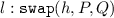• , to swap the process $P$ running at location $h$ for process $Q$.

• , to remove location $h$ from the surrounding location graph.

Concrete effects embody the reconfiguration capabilities of the G-Kells framework. Effects reconfiguring the graph itself come in pairs manifesting introduction and elimination effects: thus, adding and removing a node (location) from the graph ($\mathtt {newl}, \mathtt {kill}$), and adding and removing an edge from the graph ($\mathtt {add}, \mathtt {rmv}$). Role creation ($\mathtt {newr}$) is introduced to allow the creation of new edges. Channel creation ($\mathtt {newch}$) allows the same flexibility provided by name creation in the $\pi$-calculus. The swap effect ($\mathtt {swap}$) is introduced to allow the atomic update of a located process. The graph query effect ($\mathtt {gquery}$) is perhaps a bit more unorthodox: it allows a form of reflection whereby a location can discover part of its surrounding location graph. It is best understood as an abstraction of graph navigation and query capabilities which have been found useful for programming reconfigurations in component-based systems [11].

Operational Semantics of Location Graphs

Transitions. The operational semantics of location graphs is defined by means of a transition system, whose transition relation is defined, by means of the inference rules presented below, as a subset of . Labels take the form , where $\pi$ and $\sigma$ are located priority and synchronization constraints, respectively, and $\omega$ is a finite set of located effects (for simplicity, we reuse the same symbols than for constraints and effects). The set of labels is noted .

A located priority constraint $\pi$ is just a concrete priority constraint, and takes the form , where $I$ is a finite index set, with $l_i,r_i,a_i$ in location, role and channel names, respectively. A located synchronization constraint takes the form , where $a_j$ are channel names, $u_j$ are either location names $l_j$ or pairs of location names and roles, noted $l_j.r_j$, and $V_j$ are values. Located effects can take the following forms: , where $l,h,k$ are location names, $r$ is a role name, $P,Q$ are processes. The predicate $\mathtt {located}$ on identifies located effects. In particular, for a set , we have $\mathtt {located}(\omega )$ if and only if all elements of $\omega$ are located.

A transition is noted and must obey the following constraint:

• If , where is a set of names, and $\varDelta$ is a set of edges, then and .

• , i.e. the free names occurring in $C$ must appear in the already used names of $\varGamma$.

• If and are in , then $h = k$, i.e. we only have a single edge binding a role $r$ of a given location $l$ to another location $h$.

Auxiliary relation . The definition of makes use of an auxiliary relation , where is a set of elements of the form where $\pi$ and $\sigma$ are located priority and synchronizaton constraints, and where $\omega$ is a finite set of concrete effects. Relation is defined as the least relation satisfying the rules in Fig. 4, where we use the following notation: if , then , and if $\alpha = \epsilon$, then $l:\alpha = \epsilon$.

Rule Act simply expresses how process transitions are translated into location graph transitions, and process level constraints and effects are translated into located constraints and concrete effects, via the evaluation functions introduced above. Rule NewL specifies the effect of an effect , which creates a new location $h[Q]$. Notice how effect is removed from the set of effects in the transition label in the conclusion of the rule: auxiliary relation is in fact used to guarantee that a whole set of concrete effects are handled atomically. All the rules in Fig. 4 except Act, which just prepares for the evaluation of effects, follow the same pattern. Rules NewC and NewR specify the creation of a new channel name and of a new role name, respectively. The rules just introduce the constraint that the new name must not be an already used name in the environment $\varGamma$. Our transitions being in the early style, the use of the new name is already taken into account in the continuation location graph $C$ (in fact in the continuation process $P'$ appearing on the left hand side of the instance of rule Act that must have led to the building of $C$). This handling of new names is a bit unorthodox but it squares nicely with the explicitly indexed labelled transition semantics of the $\pi$-calculus given by Cattani and Sewell in [8]. Rule AddE specifies the effect of adding a new edge to the location graph. Rule Gquery allows the discovery by processes of a subgraph of the location graph. In the rule premise, we use the notation $\varGamma _{l}$ to denote the set of edges reachable from location $l$, formally: , where means that there exists a non-empty chain , with $n \ge 1$, linking $l$ to $h$ in the location graph $\varGamma$. As in the case of name creation rules, the exact effect on processes is left unspecified, the only constraint being that the discovered graph be indeed a subgraph of the location graph in the environment.

Fig. 4.

Rules for auxiliary relation

Fig. 5.

Rules for transition relation

Transition relation . The transition relation is defined by the rules in Fig. 5. We use the following notations and definitions in Fig. 5:

• Function is defined by induction as follows (for any $l,r,h,V,\sigma ,\sigma '$):

  

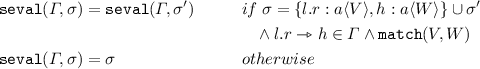
• Function is defined by induction as follows (for any $l,r,h,k,P,Q,\sigma ,\sigma '$):

  

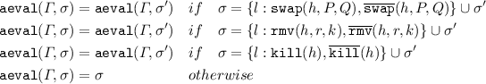
• Assume , then is obtained by replacing in $C$ all the locations with locations , where is defined by the LTS obtained from that of $P$ by the following rule:

  

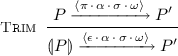
  In other terms, is obtained by disregarding the priority constraints that are generated by locations $l_i$ mentioned in the priority constraint $\pi$.

• means that, for all $i \in I$, . We write to mean that

  

Rule Swap specifies that at any point in time a location can see its process swapped for another. Likewise, rules Kill and Rmv specify that at any point in time a location or an edge, respectively, can be removed from a location graph. Rule Act specifies the termination of the atomic execution of a set of concrete effects. All the effects remaining must be located effects, which expect some counterpart (provided by the rules Swap, Kill, and Rmv, when invoking rule Comp) to proceed.

Rule Comp is the workhorse of our operational semantics of location graphs. It specifies how to determine the transitions of a parallel composition , by combining the priority constraints, synchronization constraints and effects obtained from the determination of contributing transitions from $C_1$ and $C_2$. The latter takes place in extended environment $\varGamma '$, that contains the original environment $\varGamma$, but also the edges present in $C_1$ and $C_2$, defined as $\varGamma (C_1)$ and $\varGamma (C_2)$, respectively. To ensure the names created as side effects of $C_1$ and $C_2$ transitions are indeed unique, the determination of the contributing transition of $C_1$ takes place in an environment where the already used names include those in $\varGamma$ as well as those in $\varDelta _1$, which gathers names that may be created as a side effect of the contributing transition of $C_2$. Likewise for determining the contributing transition of $C_2$. The constraint ensures that names in $\varDelta _1$ and $\varDelta _2$ are disjoint, as well as disjoint from the already used names of .

The original aspect of rule Comp lies with the computation of located synchronization constraints and effects resulting from the parallel composition of G-Kells components: we allow it to be dependent on the global environment $\varGamma '$ with the clauses and , which, in turn, allows to enforce constraints dependent on the location graph as in the definition of function . In fact, as we discuss in Sect. 4 below, we can envisage instances of the framework where different types of location-graph-dependent constraints apply.

The use of environments in rule Comp to obtain a quasi-compositional rule of evolution is reminiscent of the use of environment and process frames in the parallel rule of the $\psi$-calculus framework [3]. We say our rule Comp is quasi-compositional for the handling of priority is not compositional: it relies on the global condition , which requires computing with (an altered view of) the whole composition. The use of the operator in rule Comp is reminiscent of the handling of priorities in other works [9]. An easy way to turn rule Comp into a completely compositional rule would be to adopt a more “syntactic” approach, defining to be obtained by replacing all locations $l[P]$ in $C$ by their trimmed version , and defining environments to include information on possible actions by trimmed locations. On the other hand, we can also adopt a purely “semantic” (albeit non-compositional) variant by defining to be just $C$. However, in this case, we don’t know whether the completeness result in Theorem 1 below still stands.

Example 5

To illustrate how the rules work, consider the following process transitions:

Let , and let $\varDelta , \varDelta '$ be such that . We assume further that and , that all names $l,l_1,l_2, h, h_1$ are distinct, and that

Applying rule Act $_\bullet$, we get

Applying rule NewL, we get

Applying rule Act we get

Finally, applying rule Comp we get

Transition relation as a fixpoint. Because of the format of rule Comp, which does not prima facie obey known SOS rule formats [21], or conform to the standard notion of transition system specification [5], the question remains of which relation the rules in Figs. 4 and 5 define. Instead of trying to turn our rules into equivalent rules in an appropriate format, we answer this question directly, by providing a fixpoint definition for . We use the fixpoint construction introduced by Przymusinski for the three-valued semantics of logic programs [23].

Let be the ordering on pairs of relations in defined as:

As products of complete lattices, and are complete lattices [10]. One can read the Comp rule in Fig. 5 as the definition of an operator which operates on pairs of sub and over-approximations of . Let be the relation in obtained as the least relation satisfying the rules in Figs. 4 and  5, with rule Comp omitted. Operator is then defined as follows:

where the predicate is defined as follows:

where means that, for all $i\in I$, , and where stands for:

The definition of the predicate mimics the definition of rule Comp, with all the conditions in the premises appearing as clauses in , but where the positive transition conditions in the premises are replaced by transitions in the sub-approximation $R_1$, and negative transition conditions (appearing in the condition) are replaced by equivalent conditions with transitions not belonging to the over-approximation $R_2$. With the definitions above, if $R_1$ is a sub-approximation of , and $R_2$ is an over-approximation of , then we have and , where $\pi _1,\pi _2$ are the first and second projections. In other terms, given a pair of sub and over approximations of , computes a pair of better approximations.

From this definition, if it is easy to show that is order-preserving:

Lemma 1

For all , if , then .

Since is order-preserving, it has a least fixpoint, , by the Knaster-Tarski theorem. We can then define to be the first projection of , namely $D$. With the definition of we have adopted, and noting that it provides a form of stratification with the number of locations in a location graph with non-empty priority constraints, it is also possible to show that , meaning that as just defined is complete, using the terminology in [27]. In fact, using the terminology in [27], we can prove the theorem below, whose proof we omit for lack of space:

Theorem 1

The relation as defined above is the least well-supported model of the rules in Figs. 4 and 5. Moreover is complete.

4 Discussion

We discuss in this section the various features of the G-Kells framework and relevant related work.

Introductory example. Let’s first revisit Example 3 to see how we can further model the behavior of its different components. We can add, for instance, a crash action to the virtual machine locations, which can be triggered by a process transition at a virtual machine location of the form with the following evaluation function:

yielding, for instance, the following transition (where includes all free names in ):

This crash behavior can be extended to an arbitrary location graph residing in a virtual machine, by first discovering the location graph inside a virtual machine via the $\mathtt {gquery}$ primitive, and then killing all locations in the graph as illustrated above.

Early style. Our operational semantics for location graphs is specified in an early style [24], with values in labels manifesting the results of successful communication. This allows us to remain oblivious to the actual forms of synchronization used. For instance, one could envisage pattern matching as in the $\psi$-calculus [3], or even bi-directional pattern matching: for instance we could have a process synchronization constraint matching an offered interaction , which translate into matching located synchronization constraints and .

Mobility vs higher-order. Our operational semantics comprises both mobility features with location binding, and higher-order features with swapping and higher-order interactions. One could wonder whether these features are all needed as primitives. For instance, one could argue that mobility features are enough to model higher-order phenomena as in the $\pi$-calculus [24]. Lacking at this point a behavioral theory for the G-Kells framework, we cannot answer the question definitely here. But we doubt that mobility via location binding is sufficient to faithfully encode higher-order communication. In particular, note that we have contexts (location graphs) that can distinguish the two cases via the ability to kill locations selectively.

Directed graphs vs acyclic directed graphs. Location graphs form directed graphs. One could wonder whether to impose the additional constraints that such graphs be acyclic. While most meaningful examples of ubiquitous systems and software structures can be modeled with acyclic directed graphs, our rules for location graphs function readily with arbitrary graphs. Enforcing the constraint that all evolutions of a location graph keep it acyclic does not seem necessary.

Relationship with CAB. The G-Kells model constitutes a conservative extension of CAB. A straightforwward encoding of CAB in the G-Kells framework can be defined as in Fig. 6, with translated glues defined with the same LTS, mutatis mutandis, as CAB glues. The following proposition is then an easy consequence of our definitions:

Fig. 6.

Encoding CAB in the G-Kells framework

Proposition 1

Let $C$ be a CAB component. We have if and only if .

Graph constraints in rules. For simplicity, the evaluation functions and have been defined above with only a simple graph constraint in the first clause of the definition. One can parameterize these definitions with additional graph constraints to enforce different policies. For instance, one could constrain the use of the swap, kill and edge removal operations to locations dominating the target location by adding a constraint of the form to each of the clauses in the definition of , where means that there exists a (possibly empty) chain , linking $l$ to $h$ in the location graph $\varGamma$. Similar constraints could be added to rule AddE. Further constraints could be added to rule Gquery to further restrict the discovery of subgraphs, for instance, preventing nodes other than immediate children to be discovered.

Types and capabilities. The framework presented in this paper is an untyped one. However, introducing types similar to i/o types capabilities in the $\pi$-calculus [24] would be highly useful. For instance, edges of a location graph can be typed, perhaps with as simple a scheme as different colors to reflect different containment and visibility semantics, which can be exploited in the definition of evaluation functions to constrain effects and synchronization. In addition, location, role and channel names can be typed with capabilities constraining the transfer of rights from one location to another. For instance, transferring a location name $l$ can come with the right to swap the behavior at $l$, but not with the right to kill $l$, or with the right to bind roles of $l$ to locations, but not with the ability to swap the behavior at $l$. We believe these capabilities could be useful in enforcing encapsulation and access control policies.

Relation with the $\psi$ -calculus framework and SCEL. We already remarked that our use of environments is reminiscent of the use of frames in the $\psi$-calculus framework [3]. An important difference with the $\psi$-calculus framework is the fact that we allow interactions to depend on constraints involving the global environment, in our case the structure of the location graph. Whether one can faithfully encode the G-Kells framework (with mild linguistic assumptions on processes) with the $\psi$-calculus framework remains to be seen.

On the other hand, it would seem worthwhile to pursue the extension of the framework presented here with $\psi$-calculus-like assertions. We wonder in particular what relation the resulting framework would have with the SCEL language for autonomous and adaptive systems [12]. The notion of ensemble, being assertion-based, is more fluid than our notion of location graph, but it does not have the ability to superimpose on ensembles the kind of control actions, such as swapping and killing, that the G-Kells framework allows.

Relation with SHR. The graph manipulation capabilities embedded in the G-Kells framework are reminiscent of synchronized hyperdege replacement (SHR) systems [18]. In SHR, multiple hyperedge replacements can be synchronized to yield an atomic transformation of the underlying hypergraph in conjunction with information exchange. Intuitively, it seems one can achieve much the same effects with G-Kells: located effects can atomically build a new subgraph and modify the existing one, and they can be synchronized across multiple locations thanks to synchronization constraints. In contrast, SHR systems lack priorities and the internalization of hyperedge replacement rules (the equivalent of our processes) in graph nodes to account for inherent dynamic reconfiguration capabilities. We conjecture that SHR systems can be faithfully encoded in the G-Kells framework.

5 Conclusion

We have introduced the G-Kells framework to lift limitations in existing computational models for ubiquitous and reconfigurable software systems, in particular the ability to describe dynamic structures with sharing, where different aggregates or composites can share components. Much work remains to be done, however. We first intend to develop the behavioral theory of our framework. Indeed we hope to develop a first-order bisimulation theory for the G-Kells framework, avoiding the difficulties inherent in mixing higher-order features with passivation described in [19]. We also need to formally compare G-Kells with several other formalisms, including SHR systems and the $\psi$-calculus framework. And we definitely need to develop a typed variant of the framework to exploit the rich set of capabilities that can be attached to location names.

References

Baier, C., Sirjani, M., Arbab, F., Rutten, J.J.M.M.: Modeling component connectors in reo by constraint automata. Sci. Comput. Program. 61(2), 75–113 (2006)
Barbier, F., Henderson-Sellers, B., Le Parc, A., Bruel, J.M.: Formalization of the whole-part relationship in the unified modeling language. IEEE Trans. Softw. Eng. 29(5), 459–470 (2003)
Bengtson, J., Johansson, M., Parrow, J., Victor, B.: Psi-calculi: a framework for mobile processes with nominal data and logic. Logical Meth. Comput. Sci. 7(1) (2011)
Bliudze, S., Sifakis, J.: A notion of glue expressiveness for component-based systems. In: van Breugel, F., Chechik, M. (eds.) CONCUR 2008. LNCS, vol. 5201, pp. 508–522. Springer, Heidelberg (2008)
Bol, R.N., Groote, J.F.: The meaning of negative premises in transition system specifications. J. ACM 43(5), 863–914 (1996)
Bugliesi, M., Castagna, G., Crafa, S.: Access control for mobile agents: the calculus of boxed ambients. ACM Trans. Prog. Lang. Syst. 26(1), 57–124 (2004)
Cardelli, L., Gordon, A.: Mobile ambients. Theor. Comput. Sci. 240(1), 177–213 (2000)
Cattani, G.L., Sewell, P.: Models for name-passing processes: interleaving and causal. Inf. Comput. 190(2), 136–178 (2004)
Cleaveland, R., Lüttgen, G., Natarajan, V.: Priority in process algebra. In: Handbook of Process Algebra. Elsevier (2001)
Davey, B.A., Priestley, H.A.: Introduction to Lattices and Order, 2nd edn. Cambridge University Press, New York (2002)
David, P.C., Ledoux, T., Léger, M., Coupaye, T.: Fpath and fscript: language support for navigation and reliable reconfiguration of fractal architectures. Ann. Telecommun. 64(1–2), 45–63 (2009)
De Nicola, R., Loreti, M., Pugliese, R., Tiezzi, F.: A formal approach to autonomic systems programming: the SCEL language. ACM Trans. Auton. Adapt. Syst. 9(2), 7:1–7:29 (2014)
Di Giusto, C., Stefani, J.-B.: Revisiting glue expressiveness in component-based systems. In: De Meuter, W., Roman, G.-C. (eds.) COORDINATION 2011. LNCS, vol. 6721, pp. 16–30. Springer, Heidelberg (2011)
Ferrari, G.-L., Hirsch, D., Lanese, I., Montanari, U., Tuosto, E.: Synchronised hyperedge replacement as a model for service oriented computing. In: de Boer, F.S., Bonsangue, M.M., Graf, S., de Roever, W.-P. (eds.) FMCO 2005. LNCS, vol. 4111, pp. 22–43. Springer, Heidelberg (2006)
Fiadeiro, J.L., Lopes, A.: A model for dynamic reconfiguration in service-oriented architectures. Softw. Syst. Model. 12(2), 349–367 (2013)
Hirschkoff, D., Hirschowitz, T., Pous, D., Schmitt, A., Stefani, J.-B.: Component-oriented programming with sharing: containment is not ownership. In: Glück, R., Lowry, M. (eds.) GPCE 2005. LNCS, vol. 3676, pp. 389–404. Springer, Heidelberg (2005)
Kruchten, P.: Architectural blueprints - the 4+1 view model of software architecture. IEEE Softw. 12(6), 42–50 (1995)
Lanese, I., Montanari, U.: Mapping fusion and synchronized hyperedge replacement into logic programming. Theory Pract. Logic Program. 7(1–2), 123–151 (2007)
Lenglet, S., Schmitt, A., Stefani, J.B.: Characterizing contextual equivalence in calculi with passivation. Inf. Comput. 209(11), 1390–1433 (2011)
Milner, R.: The Space and Motion of Communicating Agents. Cambridge University Press, New York (2009)
Mousavi, M.R., Reniers, M.A., Groote, J.F.: SOS formats and meta-theory: 20 years after. Theor. Comput. Sci. 373(3), 238–272 (2007)
Oquendo, F.: \(\pi \)-ADL: an architecture description language based on the higher-order \(\pi \)-calculus for specifying dynamic and mobile software architectures. ACM Softw. Eng. Notes 29(4), 1–14 (2004)
Przymusinski, T.C.: The well-founded semantics coincides with the three-valued stable semantics. Fundamenta Informaticae 13, 445–464 (1990)
Sangiorgi, D., Walker, D.: The \(\pi \)-calculus: A Theory of Mobile Processes. Cambridge University Press, New York (2001)
Schmitt, A., Stefani, J.-B.: The kell calculus: a family of higher-order distributed process calculi. In: Priami, C., Quaglia, P. (eds.) GC 2004. LNCS, vol. 3267, pp. 146–178. Springer, Heidelberg (2005)
Tripakis, S., Stergiou, C., Shaver, C., Lee, E.A.: A modular formal semantics for ptolemy. Math. Struct. Comput. Sci. 23(4), 834–881 (2013)
van Glabbeek, R.J.: The meaning of negative premises in transition system specifications II. J. Log. Algebr. Program. 60–61, 229–258 (2004)
Wermelinger, M., Fiadeiro, J.L.: A graph transformation approach to software architecture reconfiguration. Sci. Comput. Program. 44(2), 133–155 (2002)
Ackowledgements
Damien Pous suggested the move to an early style semantics. The paper was much improved thanks to comments by Ivan Lanese on earlier versions.
Author information
Authors and Affiliations
Corresponding author
Editor information
Editors and Affiliations
Rights and permissions
Copyright information
© 2015 Springer International Publishing Switzerland
About this paper
Cite this paper
Stefani, JB. (2015). Components as Location Graphs. In: Lanese, I., Madelaine, E. (eds) Formal Aspects of Component Software. FACS 2014. Lecture Notes in Computer Science(), vol 8997. Springer, Cham. https://doi.org/10.1007/978-3-319-15317-9_1
Download citation
DOI: https://doi.org/10.1007/978-3-319-15317-9_1
Published:
Publisher Name: Springer, Cham
Print ISBN: 978-3-319-15316-2
Online ISBN: 978-3-319-15317-9
eBook Packages: Computer ScienceComputer Science (R0)