A Mathematical Theory of Financial Bubbles

Abstract

Over the last 10 years or so a mathematical theory of bubbles has emerged, in the spirit of a martingale theory based on an absence of arbitrage, as opposed to an equilibrium theory. This paper attempts to explain the major developments of the theory as it currently stands, including equities, options, forwards and futures, and foreign exchange. It also presents the recent development of a theory of bubble detection. Critiques of the theory are presented, and a defense is offered. Alternative theories, especially for bubble detection, are sketched.

Recurrent speculative insanity and the associated financial deprivation and larger devastation are, I am persuaded, inherent in the system. Perhaps it is better that this be recognized and accepted.

–John Kenneth Galbraith, A Short History of Financial Euphoria, Forward to the 1993 Edition, p. viii.

Supported in part by NSF grant DMS-0906995.

The author wishes to thank the hospitality of the Courant Institute of Mathematical Sciences, of NYU, as well as INRIA at Sophia Antipolis, for their hospitality during the writing of this paper.

These keywords were added by machine and not by the authors. This process is experimental and the keywords may be updated as the learning algorithm improves.

1 Introduction

The economic phenomenon that the popular media refers to as a financial bubble has been with us for a long time. A short adumbration of some economy wide bubbles would include the following major events (see [55] for a comprehensive history of bubbles through the ages):

• The bubble known as Tulipmania which occurred in Amsterdam in the seventeenth century (circa 1630s) is the first documented bubble of the modern era. Some merchants had excessive wealth due to Holland’s role in shipping and world commerce, and as tulips became a fad, some rare and complicated bulbs obtained through hybrid techniques led to massive speculation in the prices of bulbs. One bulb in particular came to be worth the price of two buggies with horses, the then equivalent of two automobiles. As often happens with economy wide bubbles, when the bubble burst the economy of Holland went into a tailspin.

• In the eighteenth century, John Law advised the Banque Royale (Paris, 1716–1720) to finance the crown’s war debts by selling off notes giving rights to the gold yet to be discovered in the Louisiana territories. When no gold was found, the bubble collapsed, leading to an economic catastrophe, and helped to create the French distrust of banks which lasted almost 100 years.

• Not to be outdone by the French, the South Sea Company of London (1711–1720) sold the rights to the gold pillaged from the Inca and Aztec civilizations in South America, neglecting the detail that the Spanish controlled such trade and had command of the high seas at the time. As this was realized by the British public, the bubble collapsed.

• The real king of bubbles, however, is the United States. A list of nineteenth, twentieth and now even twenty-first century bubbles would include the following, detailing only the crashes:

  • The 1816 crash due to real estate speculation.

  • With the construction of the spectacular Erie Canal connecting New York to Chicago through inland waterways, “irrational exuberance” (in the words of Alan Greenspan) led to the Crash of 1837.

  • Not having the learned its lesson in 1837, irrational exuberance due to the construction of the railroad system within the U.S. led to The Panic of 1873.

  • The Wall Street panic of October, 1907, where the market fell by 50 %, helped to solidify the fame of J.P. Morgan, who (as legend has it) stepped into the fray¹ and ended the panic by announcing he would buy everything. It also had some good effects, as its aftermath created the atmosphere that led to the creation and development of the Federal Reserve in 1913, via the Glass–Owen bill.²

  • And of course the mother of all bubbles began with Florida land speculation as people would buy swamp land that was touted as beautiful waterfront property; this then segued into massive stock market speculation, ending with The Great Crash of 1929.

  • There was no runaway speculation in the US markets, nor major panics, in the 1940s and 1950s. But it began again with minor stock market crashes in the 1960s and 1980s.

  • The marvel of “junk bond financing” led to the fame of Michael Milken, the movie Wall Street and the stock market crash of 1987.

  • While it did not occur in the U.S., we need to mention the Japanese housing bubble, circa 1970–1989, which upon bursting led to Japan’s “lost decade,” one of a stagnant economy and “zombie” banks.

  • Back to the U.S. next, where speculation due to the commercial promise of the internet led to the “dot com” crash, from March 11th, 2000 to October 9th, 2002. Many of the internet dot-coms were listed on the Nasdaq Composite index, and it lost 78 % of its value as it fell from 5,046.86 to 1,114.11; a truly dramatic crash.

  • Finally, we are all familiar with the recent US housing bubble tied to subprime mortgages, and the creation of many three letter acronym financial products, such as ABS, CDO, CDS, and even CDO². It is worth noting that the crash of 2007/2008, along with the one of 1929, escaped the economic borders of North America and thrust much of the world into economic depression.

It is of intrinsic interest to investigate the causes of financial bubbles, and there is a wealth of often insightful economic literature on the subject. This is not the purpose of this paper, which is rather to analyze prices and to try to determine if or if not a bubble is occurring, regardless of how it came about. For those with an understandable interest in the causes of bubbles, the author can recommend the little book of J.K. Galbraith [55], where Galbraith makes the case that speculation on a grand scale occurs when there is a new, or perceived as new, technological breakthrough (such as trade with the new world, the building of canals, the advent of railroads, junk bond financing, the internet, etc.) and that this can result in over enthusiasm and uncontrolled speculation. The more modern analysis of economists suggest that varied opinions among investors and short sales constraints can create financial bubbles (see for example [26, 41, 118, 138], just as a sampling). And recently, the interesting paper of Hong, Scheinkman, and Xiong [67] agrees with the conclusions of Galbraith, but takes the analysis further, beyond an explanation of simple overreaction on the part of investors to news. Hong et al. focus on the relations between investors and their advisers, the latter being classified into two types, “tech savvies” and “old fogies.” They discuss how reputation incentives create an upward bias among the recommendations of the tech savvy investors, which are taken at face value by those investors who are naïve. For an interpretation of how the recent housing bubble arose, one can consult [129]. Other interesting references are [19, 49, 139, 153, 154, 158].

To mathematically model a bubble, we start small, and consider an individual stock, rather than a sector (such as the technology sector), or an entire economy. If there is a bubble in the price of the stock, then the price is too high, relative to what one should pay for the stock. This seems intuitively obvious. But what is not obvious is: What then is the correct price of the stock? We assume such a stock is traded on an established exchange, and the theory of rational markets tells us that the price of the stock reflects exactly what the stock is worth, since if it were overvalued, people would sell it, and if it were undervalued, people would buy it. Such a theory eliminates the possibility of bubbles, and if we believe bubbles do in fact occur, we are forced not to accept this idea wholesale. Therefore we need a fair value for the stock.

This raises the question: Why does one buy a stock in the first place? Your brother-in-law might have a start-up and want you to participate by buying some stock in his company. This may be a bad investment, but good for your marriage. We will simplify life by assuming one buys stocks based only on their perceived investment potential. Moreover we will further simplify by assuming when one buys a stock, one is not speculating, and tries to pay a fair price for a long term investment, to the point where whether or not the stock goes up or down in the short run is irrelevant, and the only issue that matters is the future cash flow of the company. Nevertheless there is more of a risk in buying stocks than there is in banking money (especially when the deposits are insured by the government), so one can expect a rate of return with stocks that is higher than that of bank deposits, at least in the long run.³ This return premium for taking an extra risk to buy stocks is known as “the market price of risk.”

So the compelling question we must first answer is: How do we determine what we call a fundamental price for a stock?

1.1 Organization

After the introduction, we first explain in Sect. 2 how to model the fundamental price of a risky asset. Since the fundamental price is expressed as a conditional expectation of future cash flows, with the conditional expectation being taken under the risk neutral measure, it is more easily explained in a complete market, since then the risk neutral measure is unique. We can then define a bubble as the difference between the market price of the risky asset in question, and the fundamental price. When the risky asset is simply a stock price, then the bubbles are always nonnegative. In Sect. 3 we establish the relationship between strict local martingales⁴ and bubbles, and give a theorem classifying bubbles into three types. In Sect. 4 we give examples of mathematical models of financial bubbles by exhibiting a method of generating strict local martingales as solutions of a certain kind of stochastic differential equation. This is based on a theorem of Mijatovic and Urysov [116], and we provide a detailed proof of the theorem (Corollary 5 of Sect. 4 in this paper). Special attention is given to the inverse Bessel process. We also present results on strict local martingales in Heston type models with stochastic volatility that go beyond the framework of Corollary 5, and we discuss the multidimensional case. We end by giving a criterion to determine whether or not the system is a strict local martingale through the use of Hellinger Processes.

In Sects. 5 and 6 we consider incomplete markets arising from a risky asset price process $S = (S_{t})_{t\geq 0}$. Since incomplete markets have an infinite number of risk neutral measures, and since the fundamental price is defined using “the” risk neutral measure within the framework of complete markets, this is a bit of a thorny issue. Hence we review the method of letting the market choose the risk neutral measure originally proposed in [73] (see also [141, 142]), which works essentially by artificially completing the market through the use of call option prices. Once the risk neutral measure is chosen and temporarily fixed, the analysis proceeds analogously to the complete market case, with one important exception. The exception is that we allow the market choice of the risk neutral measure to change at random times, in a type of regime shift. This basically assumes the market is fickle, and while it always prices options in internally consistent ways (since otherwise there would be arbitrage), it can change this pricing from time to time, which actually represents a change in the selection of the risk neutral measure, from the infinite number of them compatible with the underlying risky asset price S. This method keeps the coefficients of the underlying stochastic differential equation unchanged, but we could equally and instead introduce a regime change where we change the underlying SDEs; this too may alter the structure of risk neutral measures, or it may not, depending on how dramatic is the change.

In Sect. 7 we consider what happens with calls and puts in the presence of bubbles. There are some surprising results, such as the loss of put-call parity (!) when bubbles are present, and that Merton’s “No Early Exercise” theorem for American calls no longer need hold, a fact first observed (to our knowledge) by Heston et al. [63] and by Cox and Hobson [30]. An analysis of the behavior of options in the presence of bubbles can be found in [122]. We then introduce the concept, originally due to Merton in 1973 [114] but refined mathematically successively in [88, 89], and finally in [131], and known as No Dominance. This extra assumption restores put call parity. Section 8 is devoted to a study of bubbles in foreign exchange, which is related to inflation. Here negative bubbles can occur, and Sect. 9 covers forwards and futures. Section 10 covers the controversial topic of trying to identify (in real time) when a given risky asset (such as a stock) is undergoing bubble pricing. This seems to be a question of great current interest, as the quotes given in this paragraph seem to indicate. Indeed, the quotations are from none other than Ben Bernanke (Chairman of the U.S. Federal Reserve system), William Dudley (President of the New York Federal Reserve), Charles Evans (President of the Chicago Federal Reserve), and Donald Kohn, Federal Reserve Board Vice Chairman.

Finally, in Sect. 11 we attempt to defend the local martingale approach to the study of bubbles from its critics. These criticisms seem to revolve around the use of strict local martingales, and the (technically mistaken) belief that they exist only in continuous time. Jacod and Shiryaev, in a 1998 paper [75], clarify the relationship between local martingales and generalized martingales in discrete time, and give necessary and sufficient conditions for a local martingale to be a martingale in discrete time. It is true that when a finite horizon price process in discrete time is nonnegative (such as a stock price) then as a consequence of the results of Jacod and Shiryaev, a nonnegative discrete time local martingale is indeed a martingale. So in this sense, when modeling stock prices (as we often are doing in this paper), it is indeed true that strict local martingale models do not exist for discrete time. But we argue in Sect. 11, as we have in [86], that this is just another reason of several that discrete time models are in fact inadequate to understand the full range of ideas required for a profound understanding of financial models.

We also discuss in Sect. 11 two of the leading alternative approaches to the study of bubbles, the first associated with P.C.B. Phillips and his co-authors, and the second associated with Didier Sornette and his co-authors. The key difference between these alternative approaches (of Phillips et al. and Sornette et al.) with the one presented here, is that both alternative approaches make assumptions (albeit very different ones) on the drift that leads to bubbles (under their understanding of what constitutes a bubble), whereas in our presentation the key assumptions related to bubbles revolve around the diffusive part of the model.

2 The Fundamental Price in a Complete Market

We begin with a complete probability space $(\Omega ,\mathcal{F},P)$ and a filtration $\mathbb{F} = (\mathcal{F}_{t})_{t\geq 0}$ satisfying the “usual hypotheses.”⁵ We let $r = (r_{t})_{t\geq 0}$ be at least progressively measurable, and it denotes the instantaneous default-free spot interest rate, and

$$\displaystyle{ B_{t} =\exp \left (\int _{0}^{t}r_{ u}du\right ) }$$

(1)

is then the time t value of a money market account. We work on a time interval $[0,{T}^{\star }]$ where ${T}^{\star }$ can be a finite fixed time T, or it can be ∞. We find that it is more interesting to consider a compact time interval (the finite horizon case, where ${T}^{\star } = T < \infty$), but for now let us consider the general case. Next we let τ be the lifetime of the risky asset (or stock, to be specific), where τ is a stopping time, and $\tau \leq {T}^{\star }$. τ can occur due to bankruptcy, to a buyout of the company by another company, to a merger, to being broken up by antitrust laws, etc.⁶

Next we let $D = (D_{t})_{0\leq t<\tau } \geq 0$ be the dividend process, and we assume it is a semimartingale. We let $S = (S_{t})_{0\leq t<\tau }$ be nonnegative and denote the price process of the risky asset (again, we are thinking of a stock price here), and again, we are assuming it is a semimartingale. Since S has càdlàg paths,⁷ it represents the price process ex cash flow. By ex cash flow we mean that the price at time t is after all dividends have been paid, including the time t dividend. But now we have to be a little more careful, since while the assumption that S is a semimartingale on the stochastic interval [0. τ) is necessary to exclude arbitrage opportunities, it is not sufficient. (See for example [83, 98, 127, 130]). That is, only a subclass of semimartingales exclude arbitrage opportunities. Let $\Delta \in \mathcal{F}_{\tau }$ be the time τ terminal payoff or liquidation value of the asset. We assume that $\Delta \geq 0$.

Finally, we let W be the wealth process associated with the market price of the risky asset plus accumulated cash flows:

$$\displaystyle{ W_{t} = \mathbf{1}_{\{t<\tau \}}S_{t} + B_{t}\int _{0}^{t\wedge \tau } \frac{1} {B_{u}}\mathit{dD}_{u} + \frac{B_{t}} {B_{\tau }} \Delta \mathbf{1}_{\{\tau \leq t\}}. }$$

(2)

Note that all cash flows are invested in the money market account.

It is standard (and desirable) to have a market which excludes arbitrage opportunities. There are different mathematical formulations of an arbitrage opportunity, but if one formulates them the right way then one has the validity of the first fundamental theorem of asset pricing: namely that the absence of arbitrage is mathematically equivalent to the existence of another probability measure Q, with the same null sets, that turns the price process into a martingale, or more generally a local martingale.⁸ The correct formulation for the absence of arbitrage to hold and for the first fundamental theorem to hold in full generality was established by Delbaen and Schachermayer [34, 35]. (See alternatively [127].) If is called No Free Lunch with Vanishing Risk and if often referred to by its acronym NFLVR. Note that it need not be applied directly to the price process S but can be assumed as a hypothesis relative to any risky asset in question. In our case we want to assume that NFLVR holds for the wealth process defined in (2).

Henceforth, we assume NFLVR holds (and hence there are no arbitrage opportunities) which implies there exists at least one probability measure Q, with the same null sets as P (we write Q ∼ P), such that under Q we have that W is a local martingale. We make two more assumptions, both of which will be weakened later:

• 1. The equivalent probability measure Q is unique (and hence the market is complete; see e.g. [83] and Sect. 5).

• 2. The random variable $W_{t} = \mathbf{1}_{\{t<\tau \}}S_{t} + B_{t}\int _{0}^{t\wedge \tau } \frac{1} {B_{u}}\mathit{dD}_{u} + \frac{B_{t}} {B_{\tau }} \Delta \mathbf{1}_{\{\tau \leq t\}}$ is assumed to be in L ¹(dQ) for each t, $0 \leq t \leq {T}^{\star }$.

The (now assumed to be) unique equivalent probability measure Q is often called a risk neutral measure, or the Equivalent Local Martingale Measure, sometimes abbreviated with the acronym ELMM. The term “risk neutral” comes from equilibrium theory. While individual people are risk averse when trading with their own money (and this is often mathematically modeled using utility functions), and perhaps people trading large sums with other people’s money are much less risk adverse, nevertheless the market in the whole is assumed to have risk aversion. By changing from the underlying probability P to an ELMM Q, we have an artificial transformation that generates risk neutral pricing in the market.⁹ We use this risk neutral measure to give the market’s fundamental value for the risky asset; this should be the best guess for the future discounted cash flows, given one’s knowledge at the present time. If we take conditional expectations in (2) and rearrange the terms, this translates into:

$$\displaystyle{ S_{t}^{\star } = E_{ Q}\left (\left .\int _{t}^{\tau \wedge {T}^{\star } } \frac{1} {B_{u}}\mathit{dD}_{u} + \frac{\Delta } {B_{\tau }}\mathbf{1}_{{\{\tau \leq T}^{\star }\}}\right \vert \mathcal{F}_{t}\right )B_{t}. }$$

(3)

The superscript $\star$ will be used systematically to denote fundamental values.

Definition 1.

We define β _t by

$$\displaystyle{\beta _{t} = S_{t} - S_{t}^{\star },}$$

the difference between the market price and the fundamental price. (In a well functioning market, this difference is 0.) The process β is called a bubble.

3 Characterization of Bubbles

Our first observation is that we always must have $S_{t} \geq S_{t}^{\star }$, t ≥ 0. This is of course equivalent to saying that the bubble β has the property β _t  ≥ 0 for all t, i.e., bubbles are always nonnegative.¹⁰ This is an important point, so even though it is quite simple, we formalize it as a theorem. For simplicity we consider only the case where the stock pays no dividends, and the spot interest rate is 0. Note that it is only for simplicity, and an analogous result holds if the spot rate is not 0, and also if dividends are paid. If the spot rate is not 0, one needs to discount the final term. In the case of futures however, it matters whether or not the interest rates are deterministic, or random. We treat this is Sect. 9. For dividends, there are details to keep track of (for example when the stock is ex dividend, etc.), but the ideas are the same.

Theorem 1.

Let S be the nonnegative price process of a stock and assume S pays no dividends. Moreover assume the spot interest rate is constant and equal to 0. Let Q be a risk neutral measure under which S is a local martingale (and hence a supermartingale). Let ${S}^{\star }$ be the fundamental value of the stock calculated under Q, and let $\beta _{t} = S_{t} - S_{t}^{\star }$ . Then β ≥ 0.

Proof.

Under these simplifying hypotheses of no dividends and 0 interest, the fundamental value of the stock is nothing more than

$$\displaystyle{ S_{t}^{\star } = E_{ Q}(\Delta 1_{\{\tau \leq {T}^{\star }\}}\vert \mathcal{F}_{t}). }$$

(4)

Since under Q the process S is a supermartingale, we have

$$\displaystyle{ E_{Q}(S_{\tau }\vert \mathcal{F}_{t}) \leq S_{t} }$$

(5)

and since $S_{\tau } = \Delta 1_{\{\tau \leq {T}^{\star }\}}$, combining (4) and (5) gives the result. □ 

We can classify bubbles into three types, as shown in the following theorem, which was originally proved in [88]. For this theorem, we assume fixed a risk neutral measure Q under which both S and W are local martingales.

Theorem 2.

If in an asset’s price there exists a bubble $\beta = (\beta _{t})_{t\geq 0}$ that is not identically zero, then we have three and only three possibilities:

• 1. β _t is a local martingale (which could be a uniformly integrable martingale) if $\mathbb{P}(\tau = \infty ) > 0$ .

• 2. β _t is a local martingale but not a uniformly integrable martingale if τ is unbounded, but with $\mathbb{P}(\tau < \infty ) = 1$ .

• 3. β _t is a strict $\mathbb{Q}$ -local martingale, if τ is a bounded stopping time.

Proof.

Fix Q equivalent to P such that W is a local martingale under Q. Note that W _t is a closable supermartingale, so there exists $W_{\infty }\in {L}^{1}(\mathit{dQ})$ such that W _t  → W _∞ almost surely. Also, since S is a nonnegative local martingale under the risk neutral measure, $\lim _{t\rightarrow \infty }S_{t} = S_{\infty }$ exists a.s. (cf., e.g., [128, Theorem 10, p. 8]). The fundamental wealth process is one’s best guess of future wealth, given today’s knowledge: $W_{t}^{{\ast}} = E_{Q}(W_{\infty }\vert \mathcal{F}_{t})$. Note that analogously, $W_{\infty }^{{\ast}}$ exists, and $W_{\infty } = W_{\infty }^{{\ast}}$. Let

$$\displaystyle{ \beta ^{\prime}_{t} = W_{t} - E_{Q}[W_{\infty }\vert \mathcal{F}_{t}] = W_{t} - W_{t}^{{\ast}}. }$$

(6)

Then β _t ′ is a (non-negative) local martingale since it is a difference of a local martingale and a uniformly integrable martingale. It is simple to check that

$$\displaystyle{ E_{Q}[W_{\infty }\vert \mathcal{F}_{t}] = E_{Q}[W_{\infty }^{{\ast}}\vert \mathcal{F}_{ t}] + E[S_{\infty }\vert \mathcal{F}_{t}] = W_{t}^{{\ast}} + E[S_{ \infty }\vert \mathcal{F}_{t}]. }$$

(7)

By the definition of wealth processes and (6), (7):

$$\displaystyle\begin{array}{rcl} \beta _{t}& =& S_{t} - S_{t}^{{\ast}} \\ & =& W_{t} - W_{t}^{{\ast}} \\ & =& \left (E_{Q}[W_{\infty }\vert \mathcal{F}_{t}] +\beta _{ t}^{{\prime}}\right ) -\left (E_{ Q}[W_{\infty }\vert \mathcal{F}_{t}] - E_{Q}[S_{\infty }\vert \mathcal{F}_{t}]\right ) \\ & =& \beta _{t}^{\prime} + E_{Q}[S_{\infty }\vert \mathcal{F}_{t}]. {}\end{array}$$

(8)

If τ < T for $T \in \mathbb{R}_{+}$, then S _∞  = 0. A bubble $\beta _{t} =\beta _{t}^{\prime} = 0$ for t ≥ τ and in particular β _T  = 0. If β _t is a martingale,

$$\displaystyle{ \beta _{t} = E[\beta _{T}\vert \mathcal{F}_{t}] = 0\qquad \forall t \leq T }$$

(9)

It follows that β _⋅ is a strict local martingale. This proves (1). For (2) assume that β _t is uniformly integrable martingale. Then by Doob’s optional sampling theorem, for any stopping time τ ₀ ≤ τ,

$$\displaystyle{ \beta _{\tau _{0}} = E_{Q}[\beta _{\tau }\vert \mathcal{F}_{\tau _{0}}] = 0 }$$

(10)

and since β is optional, it follows from (for example) the section theorems of P.A. Meyer (see for example [39]) that β = 0 on [0, τ]. Therefore the bubble does not exist. For (3), $E_{Q}[S_{\infty }\vert \mathcal{F}_{t}]$ is a uniformly integrable martingale and the claim holds. □ 

As indicated, there are three types of bubbles that can be present in an asset’s price. Type 1 bubbles occur when the asset has infinite life with a payoff at {τ = ∞}. Type 2 bubbles occur when the asset’s life is finite, but unbounded. Type 3 bubbles are for assets whose lives are bounded.

Of the three types of bubbles, the most interesting are those on a compact time interval, [0, T]. In this case we are dealing exclusively with Type 3 bubbles, and as seen in Theorem 2 we have that β will be a strict local martingale. Since ${S}^{\star }$ is a true martingale, and $\beta = S - {S}^{\star }$, we have that β being a strict local martingale is equivalent to the price process S being a strict local martingale. Indeed, we see that:

Corollary 1.

We have a bubble on [0,T] if and only if the price process S is a strict local martingale.

For the important special case of a bounded horizon (that is, we are working on a compact time interval, [0, T]), we can summarize as follows:

Theorem 3.

Any non-zero asset price bubble β on [0,T] is a strict Q-local martingale with the following properties:

• 1.  β ≥ 0,

• 2.  β _τ = 0,

• 3.  if β _t = 0 then β _u = 0 for all u ≥ t, and

• 4.  if no cash flows, then

  $$\displaystyle{ S_{t} = E_{Q}\left (\left .\frac{S_{T}} {B_{T}}\right \vert \mathcal{F}_{t}\right )B_{t} +\beta _{t} - E_{Q}\left (\left . \frac{\beta _{T}} {B_{T}}\right \vert \mathcal{F}_{t}\right )B_{t} }$$

  for any $\ t \leq T \leq \tau \leq {T}^{\star }$ .

This theorem states that the asset price bubble β is a strict Q- local martingale. Condition (1) states that bubbles are always non-negative, i.e. the market price can never be less than the fundamental value. Condition (2) states that the bubble must burst on or before τ. Condition (3) states that if the bubble ever bursts before the asset’s maturity, then it can never start again. Alternatively stated, condition (3) states that in the context of our model, bubbles must either exist at the start of the model, or they never will exist. And, if they exist and burst, then they cannot start again. Requiring bubbles to exist since the beginning of the modeling period is clearly a weak spot of the theory; fortunately this can be resolved within the context of incomplete markets, which allow for the concept of bubble birth. For this reason complete market models are ill suited to the study of bubbles, at least using our models of them. We will return to this subject in Sect. 6.

4 Examples of Bubbles

Of course it is of interest to know if such phenomena as bubbles occur, both in reality and in our models. We deal with our models first. Because we are working on a compact time interval, the fundamental value ${S}^{\star }$ will be a martingale as soon as $\Delta \in {L}^{1}(\mathit{dQ})$, assuming no dividends and zero interest rate. In the presence of dividends and interest rates, other assumptions on integrability with respect to a given risk neutral measure enter the picture. Therefore the existence of a bubble becomes equivalent to the stock price process being a local martingale, which is not a martingale. (The space of all local martingales includes martingales as a subspace.) However it is easy to generate local martingales. Let us make the reasonable assumption that S follows a stochastic differential equation with a unique strong solution of the rather general form

$$\displaystyle{ \mathit{dS}_{t} =\sigma (S_{t})\mathit{dB}_{t} + b(S_{t})\mathit{dt} }$$

(11)

where B is standard Brownian motion. Since Brownian motion has martingale representation, it generates complete markets (see, e.g., [83]). Therefore in this Brownian paradigm there is only one risk neutral measure Q. Under mild hypotheses on σ and b, including that σ never vanishes, (11) under Q becomes

$$\displaystyle{ \mathit{dS}_{t} =\sigma (S_{t})\mathit{dB}_{t}, }$$

(12)

and we have that S is a strict local martingale if and only if

$$\displaystyle{ \int _{\epsilon }^{\infty } \frac{x} {\sigma {(x)}^{2}}dx < \infty . }$$

(13)

for some ε > 0. This (and much more) is proved in detail in the papers [101, 116]. The idea goes back to Delbaen and Shirakawa [38]; see also [69]. However this is also easy to prove directly, using Feller’s test for explosions. We have the following results, which are based on remarks made to us by Dmitry Kramkov [102]. Theorem 4 is classic:

Theorem 4.

Let S be a nonnegative Q local martingale with S ₀ = 1. Then S is a true martingale if and only if there exists a probability measure R, with R ≪ Q, and $\frac{\mathit{dR}} {\mathit{dQ}}\vert _{\mathcal{F}_{t}} = S_{t}$ ; otherwise S is a strict local martingale.

The intuition behind why Theorem 4 is true, is that S has to have an expectation constant in time (and equal to one) in order to be a true martingale. Since it is nonnegative, this turns out also to be sufficient. If the expectation decreases with time, then R would be a sub probability measure, but not a true probability measure: some “mass would escape to ∞.”

Following Jacod and Shiryaev [76, pp. 166ff], for a stopping time ν we let P _ν denote the restriction of P to the sigma algebra $\mathcal{F}_{\nu }$, and we define R ≪ _loc Q if there exists a sequence of stopping times τ _n of stopping times such that $\tau _{n} \nearrow \infty$ a.s. and $R_{\tau _{n}} \ll P_{\tau _{n}}$ for each n. With the hypotheses of Theorem 4 one has automatically that R ≪ _loc Q. Indeed, we have a true martingale when R ≪ Q without the “local” caveat. Using Feller’s test for explosions for one dimensional diffusions (see [97, 109] as in the recent treatment in [117]), we find the criterion of Mijatovic and Urusov [116, Corollary 4.3].

Theorem 5.

Let B be a Q Brownian motion and let S be of the form

$$\displaystyle{ \mathit{dS}_{t} = S_{t}a(S_{t})\mathit{dB}_{t},\text{ under }Q. }$$

(14)

Then S is a martingale if and only if

$$\displaystyle{\int _{1}^{\infty } \frac{1} {xa{(x)}^{2}}dx =\int _{ 1}^{\infty } \frac{x} {\sigma {(x)}^{2}}dx = \infty }$$

where σ(x) = xa(x).

Proof.

By Girsanov’s theorem, (14), under R becomes

$$\displaystyle{\mathit{dS}_{t} = S_{t}a(S_{t})d\beta _{t} + S_{t}a{(S_{t})}^{2}\mathit{dt},\quad S_{ 0} = 1}$$

for an R Brownian motion β. Mijatovic and Urusov show (though they are not the first to do something like this) that S is a true martingale if and only if $\int _{0}^{t}a{(S_{s})}^{2}\mathit{ds} < \infty$ a.s. (dQ). This implies S cannot explode. To use Feller’s test to see if S explodes, we use the notation of Karatzas and Shreve [97]. Simple calculations show that in this case their scale function p is given by $p(x) = -\frac{1} {x} + C$, and their speed measure m is

$$\displaystyle{m(dx) = \frac{2dx} {{p}^{{\prime}}{(x)\sigma }^{2}(x)} ={ \frac{2{x}^{2}} {\sigma }^{2}(x)}dx.}$$

Finally their function $v(x) =\int _{ c}^{x}\left (p(x) - p(y)\right )m(\mathit{dy})$ equals

$$\displaystyle\begin{array}{rcl} & =& \int _{c}^{x}\left (-\frac{1} {x} + \frac{1} {y}\right ) \cdot { \frac{2{y}^{2}} {\sigma }^{2}(y)}dy {}\\ & =& 2\int _{c}^{x}\frac{x - y} {xy} \cdot { \frac{{y}^{2}} {\sigma }^{2}(y)}dy {}\\ & =& 2\int _{c}^{x}{ \frac{y} {\sigma }^{2}(y)}dy -\frac{2} {x}\int _{c}^{x}{ \frac{{y}^{2}} {\sigma }^{2}(y)}dy {}\\ \end{array}$$

and since in the second integral we have $\frac{y} {x} < 1$ we get that $v(+\infty ) = +\infty$ if and only if $\int _{c}^{\infty }{ \frac{y} {\sigma }^{2}(y)}\mathit{dy} = +\infty$. Taking σ(x) = xa(x) means in this context

$$\displaystyle{\int _{c}^{\infty } \frac{y} {{y}^{2}a{(y)}^{2}}\mathit{dy} =\int _{ c}^{\infty } \frac{1} {ya{(y)}^{2}}\mathit{dy} = +\infty .}$$

Therefore we see that by Feller’s test S does not explode if and only if $\int _{1}^{\infty } \frac{1} {xa{(x)}^{2}} \mathit{dx} = +\infty$, and we are done. □ 

We end this discussion by noting that we do not really need to use Feller’s test, but could have instead used the local time-space formula of stochastic calculus (see for example [128]). Namely we have that

$$\displaystyle{\int _{0}^{T}a{(S_{ s})}^{2}ds =\int _{ 0}^{\infty }a{(x)}^{2}L_{ T}^{x}dx}$$

where $L_{T}^{x}$ is the local time in x at time T of S. Since for almost all ω we have $x\mapsto L_{T}^{x}(\omega )$ is a continuous function of x that vanishes off a compact set, and if the function a never vanishes, we can conclude $0 <\epsilon (\omega ) \leq L_{T}^{x}(\omega ) < K(\omega ) < \infty$ and once again we can deduce the result. This approach is developed in detail in [116].

Of course one can ask for examples of bubbles coming from the markets. For economy wide bubbles there are many, as we mentioned in the introduction. In the case of individual assets, we detail examples in Sect. 10 later in this paper. A recent paper of X. Li, M. Lipkin, and R. Sowers [106] has shown a way in which bubbles can arise as a consequence of short squeezes related to bankruptcy stocks. There are of course many more examples, as a simple Google Scholar search will exhibit. Strict local martingales have received attention in the mathematical literature irrespective of their connection to models of financial bubbles. See for example [46, 137, 146].

4.1 Simulations for the Inverse Bessel Process

The inverse Bessel process is perhaps the most famous (or infamous) strict local martingale. It goes back at least to the renowned 1963 paper of Johnson and Helms [93] who gave it to provide an example of a nonnegative supermartingale which is uniformly integrable but is not of “Class D”, the class proposed by P.A. Meyer when he solved Doob’s decomposition conjecture, by showing it did not hold in full generality, but that it did nevertheless hold for supermartingales of Class D (the theorem is now known as the Doob–Meyer Decomposition Theorem of Supermartingales). The construction of Johnson and Helms is now classical: Let W be a standard three dimensional Brownian motion starting from the point (1, 0, 0). Let $u(p) = 1/r$, where $r =\parallel p \parallel$, the Euclidean distance of $p \in {\mathbb{R}}^{3}$ to the origin. Define a process X by X _t  = u(W _t ) for t ≥ 0. That is,

$$\displaystyle{ X_{t} = \frac{1} {\parallel W_{t} \parallel }. }$$

(15)

Then X is a uniformly integrable nonnegative process, with finite values a.s. because W never hits the origin with probability 1, and Itô’s formula shows that X is a local martingale, because u is the Newtonian potential and therefore a harmonic function for Brownian motion in ${\mathbb{R}}^{3}$. However simple calculations show that $t\mapsto E(X_{t})$ is not constant (these calculations are given in detail in the little book of Chung and Williams [29]) and indeed E(X ₀) = 1 while lim _{t → ∞} E(X _t ) = 0. An alternate representation for the inverse Bessel process is as a solution to a stochastic differential equation of the form

$$\displaystyle{ \mathit{dX}_{t} = -X_{t}^{2}\mathit{dB}_{ t};\quad X_{0} = 1 }$$

(16)

where B is a standard one dimensional Brownian motion, and therefore since (16) is of the form of Corollary 5, we know from the Mijatovic–Urysov theorem that X is a strict local martingale. Nevertheless, it is easier to simulate paths of X using the representation given in (15), so it is nice to have both methods of representing X. One can see the two representations [(15) and (16)] of X are equivalent by applying Itô’s formula to the X given in (15).

To show that the inverse Bessel process has paths that can behave as if they are paths of a stock price with bubbles, we have the following simulations¹¹ (Fig. 1).

Fig. 1

Five simulated sample paths of the inverse Bessel process

Note that a roughly half of the simulations of the sample paths of the inverse Bessel could reasonably represent a history of the price of a stock that underwent bubble pricing. For clarity, we isolate one of these paths in Fig. 2:

Fig. 2

An inverse Bessel sample path

4.2 Simulations for Stochastic Differential Equations

It is nice to go beyond the canonical case of the inverse Bessel process, and to consider other simple models of local martingales, to see if their simulations agree with one’s expectations for a model of a bubble price process. The theory tells us that they should, but one can always ask: Do simulations back up the theory? In this respect we are grateful to Jing Guo, who (at our request) simulated solutions of SDEs of the form

$$\displaystyle{\mathit{dX}_{t} = X_{t}^{1+\alpha }\mathit{dB}_{ t}}$$

for various values of α, with of course α > 0 always. One of his observations is that as α grows, the bubble peaks get more peaked: that is, they both get higher, and they also get narrower. Figure 3 below illustrates what happens, with a graph of the average of 24 paths, for α = 0. 3:

Fig. 3

Average of 24 paths with α = 0. 03

Note that we have not included the drift in the models used for these pictures, and yet certainly in practice there is a drift, as far as the data is concerned. (The dynamics under the risk neutral measure removes the drift, but the data should reflect the dynamics under the objective measure, not the risk neutral measure.) When a drift is present, it should diminish the future peaks that the simulations show occur after the initial primary peak, but we are not including here even more simulations in order to illustrate that.

4.3 The Case of Stochastic Volatility

While the examples provided by equations of type (11) form a wide and useful class of equations, several examples that include stochastic volatility already exist in the literature. They provide examples of strict local martingales (and hence bubbles on a compact time interval [0, T]) for models with stochastic volatility.

Theorem 6 (Sin). 

Assume there are no cash flows on the underlying asset, B is as in (2), that (W ¹ ,W ² ) is a standard two dimensional Brownian motion, and let $(S_{t},v_{t})$ satisfy

$$\displaystyle\begin{array}{rcl} \frac{\mathit{dS}_{t}} {S_{t}} & =& r_{t}\mathit{dt} + v_{t}^{\alpha }\left (\sigma _{ 1}\mathit{dW }_{t}^{1} +\sigma _{ 2}\mathit{dW }_{t}^{2}\right ) {}\\ \frac{\mathit{dv}_{t}} {v_{t}} & =& \rho (b - v_{t})dt + a_{1}\mathit{dW }_{t}^{1} + a_{ 2}\mathit{dW }_{t}^{2} {}\\ \end{array}$$

under the risk neutral measure Q where S ₀ = x, v ₀ = 1, α > 0, ρ ≥ 0, b > 0, a ₁ , σ ₁ , a ₂ , σ ₂ are constants. Then, $\frac{S_{t}} {B_{t}}$ is a strict local martingale under Q if and only if $a_{1}\sigma _{1} + a_{2}\sigma _{2} > 0$ .

For another example in this vein the reader can consult the work of B. Jourdain [94]. Also, L. Andersen and V. Piterbarg [3], of Bank of America and Barclay’s Capital respectively, consider a class of stochastic volatility models of the form

$$\displaystyle\begin{array}{rcl} dX_{t}& =& \lambda X_{t}\sqrt{V _{t}}dW_{t}^{1} \\ dV _{t}& =& \kappa (\theta -V _{t})dt +\epsilon V _{t}^{p}dW_{ t}^{2}{}\end{array}$$

(17)

where $({W}^{1},{W}^{2})$ is a two dimensional Brownian motion with correlation coefficient ρ.

Note that this is a generalization of the model of Sin above, and adds the feature that the correlation coefficient of the noise processes plays an important role. Anderson and Piterbarg in [3] are not trying to determine if a process is in a bubble or not, but rather their main thrust is to determine if extensions of what is known as the Heston model, a simple model using stochastic volatility, are reasonable in a financial context or not; they find that it depends on a range of parameters. And almost in passing, they discover a characterization of when the model forms a true martingale, or is a strict local martingale. This inter alia provides a simple test to determine if a process in their context is a strict local martingale, or a true martingale. They establish the following result, among many others.

Theorem 7 (Andersen–Piterbarg). 

For the model (17) above, if $p \leq \frac{1} {2}$ or $p > \frac{3} {2}$ then X is a true martingale, and if $\frac{3} {2} > p > \frac{1} {2}$ , X is a true martingale for ρ ≤ 0 and it is a strict local martingale for ρ > 0. For the case $p = \frac{3} {2}$ , X is a true martingale for $\rho \leq { \frac{1} {2}\epsilon \lambda }^{-1}$ , and X is a strict local martingale for $\rho >{ \frac{1} {2}\epsilon \lambda }^{-1}$

Perhaps the most definitive result already existing in the literature is that of P.L. Lions and M. Musiela [107]. Indeed, in their interesting paper they prove the results in Theorem 8 and in the more general result Theorem 9.

Theorem 8 (Lions–Musiela). 

Let $Z_{t} =\rho W_{t} + \sqrt{1 {-\rho }^{2}}B_{t}$ where $(W_{t},B_{t})$ is a standard two dimensional Brownian motion, and let (F,σ) solve

$$\displaystyle\begin{array}{rcl} \mathit{dF}_{t}& =& \sigma _{t}F_{t}dW_{t},\quad F_{0} = F > 0{}\end{array}$$

(18)

$$\displaystyle\begin{array}{rcl} d\sigma _{t}& =& \mu (\sigma _{t})dZ_{t} + b(\sigma _{t})dt,\quad \sigma _{0}-\sigma \geq 0{}\end{array}$$

(19)

with

$$\displaystyle\begin{array}{rcl} \mu (0)& =& 0,\quad b(0) \geq 0{}\end{array}$$

(20)

$$\displaystyle\begin{array}{rcl} \mu (\xi )& >& 0,\quad \text{ for }\xi > 0,\text{ and }\mu \text{ is Lipschitz on }[0,\infty ){}\end{array}$$

(21)

$$\displaystyle\begin{array}{rcl} b(\xi )& \leq & C(1+\xi )\text{ on }[0,\infty ),\text{ for some }C \geq 0{}\end{array}$$

(22)

Suppose in addition that the following condition holds

$$\displaystyle{ \limsup _{\xi \rightarrow \infty }{(\rho \mu (\xi )\xi + b(\xi ))\xi }^{-1} < \infty }$$

(23)

then $E(F_{t}\vert \ln F_{t}\vert ) < \infty ,E(\sup _{0\leq s\leq t}\vert F_{s}\vert ) < \infty$ for all t ≥ 0 and F _t is an integrable nonnegative martingale. On the other hand, if the following holds:

$$\displaystyle{ \liminf _{\xi \rightarrow \infty }(\rho \mu (\xi )\xi + b(\xi )) \frac{1} {\phi (\xi )} > 0 }$$

(24)

for some smooth, positive, increasing function ϕ such that $\int _{\epsilon }^{\infty }\frac{1} {\phi (\xi )}d\xi < \infty$ , for all ε > 0, then F _t is a strict local martingale, and we have $E(F_{t}) < F_{0}$ for all t > 0.

We observe that in the special case that b = 0 and μ(ξ) = αξ with α > 0, then (23) is equivalent to ρ ≤ 0, while (24) is equivalent to ρ > 0 (take ϕ(ξ) = ξ ²). Therefore we see that the correlation coefficient ρ plays an important role in determining whether or not the process $(F_{t})_{t\geq 0}$ is a strict local martingale.

Lions and Musiela go on to consider a more general case than that of Theorem 8. Instead of (18) and (19), they consider the equations

$$\displaystyle\begin{array}{rcl} \mathit{dF}_{t}& =& \sigma _{t}^{\delta }F_{ t}dW_{t},\quad F_{0} = F > 0{}\end{array}$$

(25)

$$\displaystyle\begin{array}{rcl} d\sigma _{t}& =& \gamma \sigma _{t}^{\gamma }dZ_{ t} + b(\sigma _{t})dt,\quad \sigma _{0} =\sigma > 0{}\end{array}$$

(26)

and again they want conditions under which F _t is a martingale, and conditions under which F _t is a strict local martingale. Their reasons for such an analysis are again not really related to bubble detection, but instead address the important issue as to whether or not certain stochastic volatility models are “well posed or not.” As with Anderson and Piterbarg, in Theorem 7, they provide, inter alia, a parametric framework for detecting whether or not a process is a martingale or a local martingale, based an a range of parameter values. We have the following theorem:

Theorem 9 (Lions–Musiela). 

With $(F_{t})_{t\geq 0}$ given by  (25) and  (26) , and W and Z given as in Theorem 8,

• 1. If ρ > 0 and if γ + δ > 1, we assume that b satisfies

  $$\displaystyle{ \limsup _{\xi \rightarrow \infty }\frac{b(\xi ) {+\rho \alpha \xi }^{\gamma +\delta }} {\xi } < \infty . }$$

  (27)

  Then $(F_{t})_{t\geq 0}$ is an integrable nonnegative martingale and

  $$\displaystyle{E(F_{t}\vert \ln F_{t}\vert ) < \infty ,\quad E(\sup _{0\leq s\leq t}\vert F_{s}\vert ) < \infty \quad \text{ for all }t \geq 0.}$$

• 2. If ρ > 0,γ + δ > 1 and b satisfies

  $$\displaystyle{ \liminf _{\xi \rightarrow \infty }\frac{b(\xi ){_{\rho }\alpha \xi }^{\gamma +\delta }} {\phi (\xi )} > 0 }$$

  (28)

  for some smooth, positive, increasing function ϕ such that $\int _{\epsilon }^{\infty }\frac{1} {\phi (\xi )}d\xi < \infty$ , then $(F_{t})_{t\geq 0}$ is a strict local martingale (and not a true martingale), and we have $E(F_{t}) < E(F_{0})$ for all t > 0.

4.4 Removal of Drift in the Multidimensional Case, and Strict Local Martingales

The multidimensional case is intrinsically interesting, since it is easy to imagine contagion within bubbles. The most obvious case might be that instead of an individual stock undergoing bubble pricing, the phenomenon might apply to an entire financial sector, such as technology stocks, automotive stocks, telecommunications, etc. Therefore it is interesting to understand some examples of multidimensional bubbles.

Since we know from the one dimensional case that strict local martingales are more likely if the coefficient σ increases quickly to ∞, we assume that σ is only locally Lipchitz. This guarantees existence and uniqueness of solutions up to an explosion time ξ, which can be ∞ but need not be in general. Let J = (0, ∞) and J _i be the ith copy of J, and let $I = \Pi _{i=1}^{d}J_{i}$, a subset of ${\mathbb{R}}^{d}$. We let

$$\displaystyle\begin{array}{rcl} \mu & :& I \rightarrow {\mathbb{R}}^{d} \\ \sigma & :& I \rightarrow {\mathbb{R}}^{d} \star {\mathbb{R}}^{d}{}\end{array}$$

(29)

where μ and σ are locally Lipschitz functions. We let W denote a d dimensional Brownian motion, and then our stochastic differential equation takes the usual form

$$\displaystyle{ \mathit{dS}_{t} =\mu (S_{t})\mathit{dt}+\sigma (S_{t})\mathit{dW }_{t},\text{ for }t <\xi ,\text{ where }\xi \mbox{ is a possibly infinite explosion time.} }$$

(30)

We make the hypotheses that the solution process Slives in the positive orthant.

The simplest case is to assume the square matrix σ is invertible. Then we can find a vector δ such that $\sigma \times \delta = -\mu$. We also assume that δ is locally bounded. Our candidate Radon Nikodym process will as usual be an exponential local martingale:

$$\displaystyle{ Z_{t} = {e}^{\int _{0}^{\xi \wedge t}\delta (S_{ s})dW_{s}-\frac{1} {2} \int _{0}^{\xi \wedge t}\parallel \delta (S_{ s}){\parallel }^{2}ds }, }$$

(31)

where we set Z _t  = 0 on {t ≥ ξ}.

We assume that $\int _{0}^{\xi \wedge t} \parallel \delta (S_{s}) {\parallel }^{2}\mathit{ds} < \infty$ on the event {t < ξ}, so that Z is well defined. Z is of course a nonnegative local martingale (since it solves a multidimensional exponential equation, with driving term being a continuous stochastic integral), hence (by Fatou’s Lemma) a supermartingale, and since the time horizon T is fixed, we have

$$\displaystyle{Z = (Z_{t})_{0\leq t\leq T}\text{ is a martingale, if and only if }E(Z_{T}) = 1.}$$

Note that since we are in a multidimensional Brownian paradigm, by (for example) the Kunita–Watanabe version of the martingale representation theorem, we know that all local martingales have continuous paths, and cannot therefore jump to 0, even at the time T. (See for example [128, Theorem 43, p. 188].)

We next use a technique present in the book by Karatzas and Shreve [97, Exercise 5.38, p. 352] for one dimension, and developed in much more generality and for multiple dimensions in Cheridito et al. [27]. We repeat it here since for our case, the argument is perhaps easier to follow than the more general one treated in [27]. We let

$$\displaystyle{\tau _{n} =\inf \{ t > 0\vert S_{t}\notin {[ \frac{1} {n},n]}^{d}\},}$$

the first exit time from the solid ${[ \frac{1} {n},n]}^{d}$. Note that τ _n  ↗ ↗ ξ as n → ∞, where τ _n  < ξ for each n. We next modify μ and σ, calling the new coefficients μ _n and σ _n , where μ _n and σ _n agree with μ and σ on ${[ \frac{1} {n},n]}^{d}$, and also are globally Lipschitz, and σ _n is also invertible. We then have that there exists a unique, everywhere defined, and nonnegative solution S ⁿ of the auxiliary equation

$$\displaystyle{ \mathit{dS}_{t}^{n} =\mu _{ n}(S_{s}^{n})\mathit{ds} +\sigma _{ n}(S_{s}^{n})\mathit{dB}_{ s}, }$$

(32)

where B is again a Brownian motion. Next we define δ _n such that $\sigma _{n} \times \delta _{n} = -\mu _{n}$, and define

$$\displaystyle{L_{t}^{n} =\int _{ 0}^{\tau _{n}\wedge t} -\delta _{ n}(S_{s}^{n})\mathit{dB}_{ s}}$$

which is well defined globally since L ⁿ is a local martingale with

$$\displaystyle{[{L}^{n},{L}^{n}]_{ t} =\int _{ 0}^{t\wedge \tau _{n} } \parallel \delta {\parallel }^{2}(S_{ s}^{n})\mathit{ds} \leq \parallel \delta \parallel _{{ L}^{\infty },[ \frac{1} {n},n]}^{2}t < \infty }$$

and hence $[{L}^{n},{L}^{n}]_{t} \in {L}^{1}$ and L ⁿ is actually a (true) square integrable martingale. However by Novikov’s criterion (see for example [128]) we also have that the stochastic (also known as the Doléans–Dade) exponential $\mathcal{E}({L}^{n})$ is a martingale. We let

$$\displaystyle{D_{t}^{n} = D_{ 0}\mathcal{E}(L_{t}^{n})\text{ for }t <\xi ,\text{ and }D_{\xi }^{n} =\lim _{ n\rightarrow \infty }D_{\tau _{n}}^{n}}$$

and again, D ⁿ is a (nonnegative) martingale, so there is no problem in asserting the limit above exists. D ⁿ so defined is a supermartingale, by Fatou’s Lemma. We next relate it to the process Z defined in (31). For n ≥ m we have $D_{t}^{n} = D_{t}^{m}\text{ for }t \leq \tau _{m}$, and hence for t < ξ we define $D_{t} =\lim D_{t}^{n} \geq 0$, as n → ∞. Note that D _t  > 0 on {t < ξ} ∩ { D ₀ > 0}. Finally, for t < ξ we have $D_{t} = D_{0} \frac{Z_{t}} {Z_{0}}$. All this is preamble to defining a sequence of new measures:

$$\displaystyle{\frac{d{Q}^{n}} {dP} \vert _{\mathcal{F}_{\tau _{n}}} = \frac{D_{\tau _{n}}} {D_{0}} .}$$

Using Girsanov’s theorem we have that $W_{t}^{n} = W_{t} +\int _{ 0}^{t\wedge \tau _{n}}\delta (S_{s}^{n})\mathit{ds}$ is a Q ⁿ Brownian motion up to τ _n , giving rise to the SDE system (up to time τ _n ):

$$\displaystyle\begin{array}{rcl} \mathit{dW }_{t}^{n}& =& \mathit{dW }_{ t} +\delta (S_{t}^{n})\mathit{dt} {}\\ \mathit{dS}_{t}^{n}& =& \sigma (S_{ t}^{n})\mathit{dW }_{ t}^{n} {}\\ \end{array}$$

and using the uniqueness in law of the solutions we have that the Q ⁿ measures are compatible and give an über measure Q with ${Q}^{n} = Q\vert _{\mathcal{F}_{\tau _{n}}}$ for each n, with

$$\displaystyle{ \frac{dQ} {dP}\vert _{\mathcal{F}_{\tau _{n}}} = \frac{D_{\tau _{n}}} {D_{0}} \text{ and }Q_{\vert _{\mathcal{F}_{\tau _{ n}}}}^{n} = Q_{\vert _{ \mathcal{F}_{\tau _{n}}}}. }$$

(33)

Theorem 10.

With Z,Q, as defined above, and ξ the explosion time of S, we have

$$\displaystyle{E_{P}(Z_{T}1_{\{\xi >T\}}) = Q(\xi > T).}$$

Proof.

Let $A \in \mathcal{F}_{T}$. Recalling that D = Z a.s. on the event {T < ξ}, we have:

$$\displaystyle\begin{array}{rcl} E_{P}(Z_{T}1_{\{T<\xi \}}1_{A})& =& E_{P}(\frac{D_{T}} {D_{0}} 1_{\{T<\xi \}}1_{A}) {}\\ & =& E_{P}(\frac{D_{T}} {D_{0}} \lim _{n\rightarrow \infty }1_{\{T<\tau _{n}\}}1_{A}) {}\\ & =& \lim _{n\rightarrow \infty }E_{P}(\frac{D_{T}} {D_{0}} 1_{\{T<\tau _{n}\}}1_{A}) {}\\ & & \mbox{ by the monotone convergence theorem; and using that } {}\\ & & D_{T} = D_{T\wedge \tau _{n}}\text{ on }1_{\{T<\tau _{n}\}},\mbox{ the above equals } {}\\ & =& \lim _{n\rightarrow \infty }E_{Q}(1_{\{T<\tau _{n}\}}1_{A}) {}\\ & =& Q(A \cap T <\xi ) {}\\ \end{array}$$

again by the monotone convergence theorem. The theorem follows by taking $A = \Omega$. □ 

Corollary 2.

Let S be as given in  (30) and Z be as given in  (31) . With the notation and assumptions of Theorem 10, if S does not explode under Q, then Z is a true martingale. If S does not explode under P, then Z is a martingale if and only if S does not explode under Q.

Proof.

Let us first assume that S does not explode under Q. But Z is a martingale if and only if E(Z _T ) = 1, and this happens if and only if Q(ξ > T) = 1. Next we suppose that S does not explode under P. Then Z is a supermartingale, so $E_{P}(Z_{T}) \leq 1$. Therefore if S does not explode under Q, we have $E_{P}(Z_{T}1_{\{\xi >T\}}) = 1$. However since $E_{P}(Z_{T}) \leq 1$, and Z _T  = 0 on {T ≥ ξ} a.s., we deduce the result. □ 

Why do we care whether or not Z is a martingale or only a local martingale? We know that the solution S of (30) is nonnegative and let us suppose it does not explode under P. We know that under a risk neutral measure the drift disappears and S is always a vector of at least local martingales, and it is a vector of martingales if and only if S does not explode in each of every component, and as we have seen by Corollary 2, this is tied to whether or not Z is a martingale. This is nice to know, but it is not much help in analyzing whether or not a given system is a martingale or a strict local martingale, the key property for telling whether or not we have a financial bubble.

We next give a criterion to determine whether or not the system is a strict local martingale through the use of Hellinger Processes. We use freely results about Hellinger Processes from the book of Jacod and Shiryaev [76]. First we note that if Q and P are two probabilities, we can define $R = \frac{P+Q} {2}$ and then P ≪ R and Q ≪ R. We let $X = \frac{\mathit{dP}} {\mathit{dR}}$ and $Y = \frac{\mathit{dQ}} {\mathit{dR}}$, with X = (X _t ) _t ≥ 0 and Y = (Y _t ) _t ≥ 0 being their respective martingale versions, through projections onto the filtration. We set $U_{t} = \frac{X_{t}} {Y _{t}}$, and define

$$\displaystyle{ \alpha _{t} = \left \{\begin{array}{r@{\quad \text {if}\quad }l} \frac{X_{t}} {Y _{t}} \quad \text{if}\quad &0 < U_{t-} < \infty \\ 0\quad \text{if}\quad &U_{t-} = 0 \\ \infty \quad \text{if}\quad &U_{t-} = \infty \end{array} \right . }$$

(34)

While we do not reproduce the proof here, Younes Kchia has shown  (2011, private communication):

Theorem 11.

Let the process Z be given as in  (31) , the process α be as given in  (34) , and the probability Q be as given in  (33) . We then have that Z is a true martingale if and only if $Q(h(\frac{1} {2})_{T} < \infty ) = 1$ and Q(sup _0≤t≤T α _t < ∞) = 1. Here $h(\frac{1} {2})_{T}$ is the Hellinger process of order $\frac{1} {2}$ between P and Q.

We note that in the case considered above, if all processes are continuous and using $R = \frac{P+Q} {2}$, we have

$$\displaystyle{h(\frac{1} {2}) = \frac{1} {8}{\left ( \frac{1} {X} + \frac{1} {Y }\right )}^{2} \cdot [X,X].}$$

(See for example [76, p. 236].) We also note that these are much less practical conditions to check than those we have in the one dimensional case. We will see later that the one dimensional case presents its own formidable problems if we want to check if a condition such as (13) holds, in order to determine whether or not S is a strict local martingale.

For more ways to generate strict local martingales, as well as a study of their asymptotic behaviors, we refer the interested reader to [122]. Related papers involving strict local martingales include [11, 15, 30, 50, 96, 108], as well as the recent book [124].

5 Incomplete Markets: Choosing a Risk Neutral Measure

When we consider incomplete markets we immediately have a problem: How do we choose a risk neutral measure so that we can well define the fundamental value of a risky asset? The Second Fundamental Theorem of Finance states that a market is incomplete if and only if there exists an infinite number of equivalent risk neutral measures (see, e.g., [37], or [83]), so the question is not a trivial one. Many different methods have been proposed to solve this question, including (with sample references) indifference pricing (see for example the volume edited by R. Carmona [20]), choosing a risk neutral measure by choosing one that minimizes the entropy (or alternatively the “distance”) between the objective measure and the class of risk neutral measures (see for example the excellent paper of Grandits and Rheinlander [60]), by minimizing the variance of certain terms in the semimartingale decomposition, known as choosing the minimal variance measure (see for example Föllmer–Schweizer [53], or the subsequent results of Monat and Stricker [119]). Each of these methods works but they all give the uneasy feeling of arbitrariness, whose main value is a canonical procedure to choose a risk neutral measure. Instead, and as an alternative, we will sketch here a procedure due to Jacod and this author [73], which gives conditions under which it is apparent that the market has itself chosen a unique risk neutral measure. A similar approach (with a similar result) was taken in Schweizer and Wissel [141, 142], albeit in a more restrictive case (i.e., restricted to the Brownian paradigm). When sufficient conditions hold for the uniqueness of a risk neutral measure compatible with all market prices, it seems intuitively reasonable to use that risk neutral measure for pricing purposes, since it is the one the market itself is using.

The basic idea of the article [73] is to take an inherently incomplete market, and to complete it artificially by including option prices. This is accomplished by modeling the market price S of our risky asset together with a family of traded options. In this way, the options can in theory “complete” the market, rendering the choice of a compatible risk neutral measure unique. This idea is not new with [73], and its beginnings can be traced to the late 1990s, with the works of Dengler and Jarrow [40], Dupire [43], Derman and Kani [102], and also Schönbucher [140]. Note that if one ignores the options, the model depending only on the risky asset price remains incomplete, with an infinite choice of risk neutral measures, and we call this set $\mathbb{Q}_{S}$. Therefore if the option prices change, for whatever reason, they could become compatible with a different choice of risk neutral measure in $\mathbb{Q}_{S}$, and it is this flexibility that allows us to include bubble birth in our model, in the incomplete case.

We assume the following model for the stock price X. First, in the continuous case we suppose that

$$\displaystyle{ X_{t} = X_{0} +\int _{ 0}^{t}a_{ s}ds +\sum _{i\in I}\int _{0}^{t}\sigma _{ s}^{i}\mathit{dW }_{ s}^{i}. }$$

(35)

In the general case, when there are jumps, we suppose that

$$\displaystyle{ X_{t} = X_{0} +\int _{ 0}^{t}a_{ s}ds +\sum _{i\in I}\int _{0}^{t}\sigma _{ s}^{i}dW_{ s}^{i} + (\psi 1_{\{ \vert \psi \vert \leq 1\}}) {\ast} (\mu -\nu )_{t} + (\psi 1_{\{\vert \psi \vert >1\}}) {\ast}\mu _{t}. }$$

(36)

Here we are using established notation for stochastic integrals with respect to Brownian motions W ⁱ and random measure μ, or compensated random measure μ − ν, see for example the book of Jacod and Shiryaev [76]. We assume also that ν factors: ν(dt, dx) = dtF(dx). The index set I is assumed finite. In (36) X ₀ > 0 is non-random and the coefficients a, σ ⁱ and ψ are such that the integrals and sums above make sense: that is, a and σ ⁱ are predictable and ψ is $\tilde{\mathcal{P}}$-measurable, and

$$\displaystyle{ \int _{0}^{t}\left (\vert a_{ s}\vert +\sum _{i\in I}\vert \sigma _{s}^{i}{\vert }^{2} +\int \ (\psi {(s,x)}^{2} \wedge 1)\,F(dx)\right )ds < \infty \qquad \mbox{ a.s.} }$$

(37)

for all t. (We use $\tilde{\mathcal{P}}$ to denote the product σ algebra $\mathcal{P}\otimes \mathcal{R}$ on $\Omega \times \mathbb{R}_{+} \times \mathbb{R}$.)

Of course these coefficients should also be such that X _t  > 0: this amounts to saying that they factor as $a_{t} = X_{t-}\bar{a}_{t}$ and $\sigma _{t}^{i} = X_{t-}\bar{\sigma }_{t}^{i}$ and $\psi (t,x) = X_{t-}\bar{\psi }(t,x)$ with $\bar{\psi }> -1$ identically, with $\bar{a}{,\bar{\sigma }}^{i}$ and $\bar{\psi }$ satisfying (37), but it is more convenient to use the form (36). Note that this represents the most general semimartingale driven by μ and the W ⁱ’s that has a chance to satisfy the hypotheses NFLVR (No Free Lunch with Vanishing Risk) of Delbaen and Schachermayer.

For options, we consider a fixed pay-off function g on (0, ∞) which is nonnegative and convex, and we denote by P(T) _t the price at time t ∈ [0, T] of the option with pay-off g(X _T ) at expiration date T. We also assume that g is not affine, otherwise P(T) _t  = g(X _t ) and we are in a trivial situation.

We denote by $\mathcal{T}$ the set of expiration dates T corresponding to tradable options (always with the same given pay-off function g), and by $T_{\star }$ the time horizon up to when trading may take place. Even when $T_{\star } < \infty$, there might be options with expiration date $T > T_{\star }$, so we need to specify the model up to infinity.

In practice $\mathcal{T}$ is a finite set, although perhaps quite large. For the mathematical analysis it is much more convenient to take $\mathcal{T}$ to be an interval, or perhaps a countable set which is dense in an interval. We consider the case where $T_{\star } < \infty$ and $\mathcal{T} = [T_{0},\infty )$, with $T_{0} > T_{\star }$.

Apart from the fact that P(T) _T  = g(X _T ), the prices P(T) _t are so far unspecified, and the idea is to model them on the basis of the same W ⁱ and μ, rather than with X. However, since these are option prices, they should have some internal compatibility properties.

Indeed, if the option prices were derived in the customary way, we would have a measure $\mathbb{Q}$ which is equivalent to $\mathbb{P}$, and under which X is a martingale and g(X _T ) is $\mathbb{Q}$-integrable and $P(T)_{t} = \mathbb{E}_{\mathbb{Q}}(g(X_{T})\vert \mathcal{F}_{t})$ for t ≤ T. Then of course P(T) is a $\mathbb{Q}$-martingale indexed by [0, T]. But we can also look at how P(T) _t varies as a function of the expiration date T, on the interval [t, ∞). That is, we are taking the non customary step of fixing t, and considering P(T) _t as a process where T varies. Since X is a quasi-left continuous martingale and g is convex, then $T\mapsto g(X_{T})$ is a quasi-left continuous submartingale relative to $\mathbb{Q}$, and this implies that $T\mapsto P(T)_{t}$ is non-decreasing and continuous for T ≥ t. Observe that this property holds $\mathbb{Q}$-almost surely, hence $\mathbb{P}$-almost surely as well because $\mathbb{P}$ and $\mathbb{Q}$ are equivalent.

Remark 12.

We wish to emphasize that, for example in the case of European call options, the usual theory calls for $P(T)_{t} = \mathbb{E}_{{\mathbb{Q}}^{\star }}((X_{T} - K)_{+}\vert \mathcal{F}_{t})$ for some risk neutral measure ${Q}^{\star }$. We do not make this assumption here. Indeed, the previous paragraph is simply motivation for us to assume a priori that $T\mapsto P(T)_{t}$ is non-decreasing and continuous. This seems completely reasonable from the viewpoint of practice, where (in the absence of dividends or interest rate changes and anomalies) it is always observed that $T\mapsto P(T)_{t}$ is nondecreasing. In the language of practitioners, if it were not it would imply a “negative pricing of the calendar,” which makes no economic sense  Lipkin, American stock exchange, 2007, private communication. Nevertheless we warn the reader that there are pathological examples where this assumption does not hold: for example if X is the reciprocal of a three dimensional Bessel process starting at X ₀ = 1, then X is a local martingale for its natural filtration, but $T\mapsto P(T)_{0}$ is not increasing, since P(0)₀ = 0, P(T)₀ > 0 for T ∈ (0, ∞), but lim _{T → ∞} P(T)₀ = 0, hence $T\mapsto P(T)_{0}$ cannot be increasing for T ≥ 0. Thus our assumption $T\mapsto P(T)_{t}$ is increasing in T rules out the possibility of the market being governed by such price processes. This is an important exception, since the inverse Bessel process is the classic example of a strict local martingale, going back to the paper of Johnson and Helms [93]. The inverse Bessel process is of course a canonical example of a strict local martingale, fitting into the theory of when there are bubbles, so it would seem that this particular theory is excluding precisely the case where there are bubbles in call options, a topic treated in Sect. 7. Note however that in the proofs presented in [73], the assumption that $T\mapsto P(T)_{t}$ is increasing in T is not essential, and could be replaced simply with $T\mapsto P(T)_{t}$ is absolutely continuous as a function of T. This change allows us to apply this theory to the more general case where bubbles in option prices are included.

We write

$$\displaystyle{ P(T)_{t} = P(T_{0})_{t} +\int _{ T_{0}}^{T}f(t,s)\mathit{ds}. }$$

(38)

In this case, the inverse Bessel process and other local martingales are included. The function f has the representation

$$\displaystyle\begin{array}{rcl} f(t,s)& =& f(0,s) +\int _{ 0}^{t}\alpha (u,s)\mathit{du} +\sum _{ i\in I}\int _{0}^{{t}}\gamma ^{i}(u,s)\mathit{dW }_{ u}^{i} \\ & & +(\phi (.,s)1_{\{\vert \phi (.,s)\vert \leq 1\}}) {\ast} (\mu -\nu )_{t} + (\phi (.,s)1_{\{\vert \phi (.,s)\vert >1\}}) {\ast}\mu _{t}.{}\end{array}$$

(39)

We further assume that the process P(T ₀) is given for $t \leq T_{\star }$ by

$$\displaystyle{ P(T_{0})_{t} = P(T_{0})_{0} +\int _{ 0}^{t}\overline{\alpha }_{ s}\mathit{ds} +\sum _{i\in I}\int _{0}^{t}\overline{\gamma }_{ s}^{i}\mathit{dW }_{ s}^{i} }$$

(40)

in the continuous case, and in the general case by

$$\displaystyle{ P(T_{0})_{t} = P(T_{0})_{0} +\int _{ 0}^{t}\overline{\alpha }_{ s}\mathit{ds} +\sum _{i\in I}\int _{0}^{t}\overline{\gamma }_{ s}^{i}\mathit{dW }_{ s}^{i} + (\overline{\phi }1_{\{ \vert \overline{\phi }\vert \leq 1\}}) {\ast} (\mu -\nu )_{t} + (\overline{\phi }1_{\{\vert \overline{\phi }\vert >1\}}) {\ast}\mu _{t}, }$$

(41)

where the above coefficients are predictable and satisfy

$$\displaystyle{ \int _{0}^{T_{\star } }\left (\vert \overline{\alpha }_{t}\vert +\sum _{i\in I}\vert \overline{\gamma }_{t}^{i}{\vert }^{2} +\int (\overline{\phi }{(t,x)}^{2} \wedge 1)F(dx)\right )dt < \infty }$$

(42)

a.s., and further the (non-random) initial condition P(T ₀)₀ and these coefficients are such that we have identically

$$\displaystyle{ t \in [0,T_{\star }]\quad \Rightarrow \quad P(T_{0})_{t} \geq g(X_{t}). }$$

(43)

Finally we assume that we have $\int _{T_{0}}^{T}\chi (s)_{T_{\star }}\mathit{ds} < \infty$ a.s. for all T > T ₀, where

$$\displaystyle{\chi (s)_{t} =\int _{ 0}^{t}\left (\vert \alpha (u,s)\vert +\sum _{ i\in I}{\vert \gamma }^{i}(u,s){\vert }^{2} +\int (\phi {(u,x,s)}^{2} \wedge 1)\,F(\mathit{dx})\right )\mathit{du}.}$$

An example of the type of results obtained in [73] is when trading takes place up to time $T_{\star }$, and the expiration dates of the options are all T ≥ T ₀, where $T_{0} > T_{\star }$. We denote $\mathcal{M}_{\text{loc}}(T_{\star },T_{0})$ the collection of risk neutral measures for X that are compatible with the option structure so that no arbitrage opportunities exist. The following result is shown in [73]:

Theorem 13.

Consider a $(T_{\star },T_{0})$ partial fair model such that the set $\mathcal{M}_{\text{loc}}(T_{\star },T_{0})$ is not empty. Then this set is a singleton if and only if, for a good version of the coefficients of the model, we have the following property: the system of linear equations

$$\displaystyle{ \sum _{i\in I}\sigma _{s}^{i}(\omega )\beta _{ i} +\int \psi (\omega ,s,x)y(x)\,dx = 0, }$$

(44)

$$\displaystyle{ \sum _{i\in I}\overline{\gamma }_{s}^{i}(\omega )\beta _{ i} +\int \overline{\phi }(\omega ,s,x)y(x)\,dx = 0, }$$

(45)

$$\displaystyle{ T \geq T_{0} \Rightarrow \sum {_{i\in I}\alpha }^{i}(s,T)(\omega )\beta _{ i} +\int \phi (\omega ,s,x,T)y(x)\,dx = 0, }$$

(46)

where $((\beta _{i}),y) \in \Upsilon ^{\prime}(\omega ,s)$ , has for its only solution β _i = 0 and y = 0 up to a Lebesgue-null set.

A consequence is that we see when conditions such as those in Theorem 13 above are met, the market prices for the options have uniquely determined a risk neutral measure. Also, should the market change its collective mind about the pricing of options, it could still choose a unique risk neutral measure, but a new one. Such phenomena have been noticed by economists, and it is referred to colloquially as the sun spot theory, since occasionally the sun gets sun spots, and they appear to happen randomly and without explanation (see for example [7, 22]).

6 Incomplete Markets: Bubble Birth

We use the idea of the previous section to extend our model of the economy to allow for the possibility of bubble “birth” after the model starts. A modification involves the market exhibiting different local martingale measures across time. We note that this is different from the usual paradigm of choosing an initial equivalent local martingale measure, and remaining with it fixed as our choice for all time, but we will see it is not that different from the standard notion of regime change. Indeed, shifting local martingale measures corresponds to regime shifts in the underlying economy (in any of the economy’s endowments, beliefs, risk aversion, institutional structures, or technologies). For pedagogical reasons we choose a simple and intuitive structure consistent with this extension.

To begin this extension, we need to define the regime shifting process. Let $(\sigma _{i})_{i\geq 0}$ denote an increasing sequence of random times with σ ₀ = 0. The random times $(\sigma _{i})_{i\geq 0}$ represent the times of regime shifts in the economy. It is important that these times σ _i be totally inaccessible stopping times. (See for example [128] for definitions and properties of totally inaccessible stopping times.) For if they were to be predictable, traders could see the regime shifts coming and develop arbitrage strategies around the shifts.¹² If we are working within a minimal Brownian paradigm, then there are no totally inaccessible stopping times, so we would need to consider a larger space that supports such times.

We let $({Y }^{i})_{i\geq 0}$ be a sequence of random variables characterizing the state of the economy at those times (the particular regime’s characteristics) such that $({Y }^{i})_{i\geq 0}$ and (σ) _i ≥ 0 are independent of each other. Moreover, we further assume that both $({Y }^{i})_{i\geq 0}$ and (σ) _i ≥ 0 are also independent of the underlying filtration $\mathbb{F}$ to which the price process S is adapted.

Define two stochastic processes $(N_{t})_{t\geq 0}$ and (Y _t ) _t ≥ 0 by

$$\displaystyle{ N_{t} =\sum _{i\geq 0}\mathbf{1}_{\{t\geq \sigma _{i}\}}\text{ \ \ and \ \ }Y _{t} =\sum _{i\geq 0}{Y }^{i}\mathbf{1}_{\{\sigma _{ i}\leq t<\sigma _{i+1}\}}. }$$

(47)

N _t counts the number of regime shifts up to and including time t, while Y _t identifies the characteristics of the regime at time t. Let $\mathbb{H}$ be a natural filtration generated by N and Y and define the enlarged filtration $\mathbb{G} = \mathbb{F} \vee \mathbb{H}$ (for example see [128] or [120] for a discussion of some of the general theory of filtration enlargement). By the definition of $\mathbb{G}$, $(\sigma _{i})_{i\geq 0}$ is an increasing sequence of $\mathbb{G}$ stopping times.

Since N and Y are independent of $\mathbb{F}$, every $(Q, \mathbb{F})$-local martingale is also a $(Q, \mathbb{G})$-local martingale. By this independence, changing the distribution of N and/or Y does not affect the martingale property of the wealth process W. To discuss a collection of ELMMs, however, it is prudent to work on a finite horizon ([0, T]), and not on the infinite half line [0, ∞). Therefore, we do not speak of the mathematically appealing set of ELMMs defined on $\mathcal{G}_{\infty }$, but rather we fix a (non random) horizon time T < ∞ and speak of the ELMMs defines on $\mathcal{G}_{T}$, and that is a priori larger than the set of ELMMs defined on $\mathcal{F}_{T}$. We are not concerned with this enlarged set of ELMMs. We will, instead, focus our attention on the $\mathcal{F}_{T}$ ELMMs and sometimes write $\mathcal{M}_{\mathit{loc}}^{\mathbb{F}}(W)$ to recognize explicitly this restriction. With respect to this restricted set, given the Radon Nikodym derivative $Z_{T} = \frac{\mathit{dQ}} {dP}\vert _{\mathcal{F}_{T}}$, we define its density process by $Z_{t} = E[Z_{T}\vert \mathcal{F}_{t}]$. Of course, Z is an $\mathbb{F}$-adapted process. Note that this construction implies that the distribution of Y and N is invariant with respect to a change of ELMMs in $\mathcal{M}_{\mathit{loc}}^{\mathbb{F}}(W)$.

We will henceforth always be working in this section on the finite horizon case [0, T] with the non random timeTchosen a priori and fixed. We will no longer make special mention of this implicit assumption.

The independence of the filtration $\mathbb{H}$ from $\mathbb{F}$ gives this increased randomness in our economy the interpretation of being extrinsic uncertainty. It is well known that extrinsic uncertainty can affect economic equilibrium as in the sunspot equilibrium of Cass and Shell [7, 22]. This form of our information enlargement, however, is not essential to our arguments. It could be relaxed, making both N and Y pairwise dependent, and dependent on the original filtration $\mathbb{F}$ as well. This generalization would allow bubble birth to depend on intrinsic uncertainty (see Froot and Obstfeld [54] for a related discussion of intrinsic uncertainty). However, this generalization requires a significant extension in the mathematical complexity of the notation and proofs, so we leave it aside.

We are now ready to discuss the fundamental price of a risky asset in the incomplete market context. Of course to do this, we need to select a risk neutral measure from an infinite selection of possibilities. We do this with the aid of Theorem 13. Because the unique measure specified in Theorem 13 can change as the regime shifts, so too might the fundamental value of the asset. Since the selection of the risk neutral measure affects the fundamental value, and this can change as the regime shifts, we can have the birth of price bubbles. More formally, we let the local martingale measure in our extended economy depend on the state of the economy at time t as represented by the original filtration $(\mathcal{F}_{t})_{t\geq 0}$, the state variable(s) Y _t , and the number of regime shifts N _t that have occurred. Suppose N _t  = i. Denote ${Q}^{i} \in \mathcal{M}_{\mathit{loc}}(W)$ as the ELMM “selected by the market” at time t given Y ⁱ.

As in the complete market case, the fundamental price of an asset (or portfolio) represents the asset’s expected discounted cash flows.

Definition 2 (Fundamental Price). 

Let $\phi \in \Phi$ be an asset with maturity ν and payoff $(\Delta ,{\Xi }^{\nu })$. The fundamental price $\Lambda _{t}^{\star }(\phi )$ of asset ϕ is defined by

$$\displaystyle{ \Lambda _{t}^{\star }(\phi ) =\sum _{ i=0}^{\infty }E_{{ Q}^{i}}\left [\left .\int _{t}^{\nu }d\Delta _{ u} + {\Xi }^{\nu }\mathbf{1}_{\{\nu <\infty \}}\right \vert \mathcal{F}_{t}\right ]\mathbf{1}_{\{t<\nu \}\cap \{t\in [\sigma _{i},\sigma _{i+1})\}} }$$

(48)

$\forall t \in [0,\infty )$ where $\Lambda _{\infty }^{\star }(\phi ) = 0$.

In particular the fundamental price of the risky asset $S_{t}^{\star }$ is given by

$$\displaystyle{ S_{t}^{\star } =\sum _{ i=0}^{\infty }E_{{ Q}^{i}}\left [\left .\int _{t}^{\tau }\mathit{dD}_{ u} + X_{\tau }\mathbf{1}_{\{\tau <\infty \}}\right \vert \mathcal{F}_{t}\right ]\mathbf{1}_{\{t<\tau \}\cap \{t\in [\sigma _{i},\sigma _{i+1})\}}. }$$

(49)

To understand this definition, let us focus on the risky asset’s fundamental price. At any time t < τ, given that we are in the ith regime {σ _i  ≤ t < σ _i + 1}, the right side of expression (49) simplifies to:

$$\displaystyle{ S_{t}^{\star } = E_{{ Q}^{i}}\left [\left .\int _{t}^{\tau }\mathit{dD}_{ u} + X_{\tau }\mathbf{1}_{\{\tau <\infty \}}\right \vert \mathcal{F}_{t}\right ]. }$$

Given the market’s choice of the ELMM is ${Q}^{i} \in \mathcal{M}_{\mathit{loc}}^{\mathbb{F}}(W)$ at time t, we see that the fundamental price equals its expected future cash flows. Note that the payoff of the asset at infinity, X _τ 1 _{{τ = ∞}}, does not contribute to the fundamental price. This reflects the fact that agents cannot consume the payoff X _τ 1 _{{τ = ∞}}. Furthermore note that at time τ, the fundamental price $S_{\tau }^{\star } = 0$. We emphasize that a fundamental price is not necessarily the same as the market price S _t . Under NFLVR the market price S _t equals the arbitrage-free price,¹³ but this need not equal the fundamental price $S_{t}^{\star }$.

For notational simplicity, we can alternatively rewrite the fundamental price in terms of an equivalent probability measure, indexed by time t, that is not a local martingale measure because of this time dependence.

Theorem 14.

There exists an equivalent probability measure ${Q}^{t\star }$ such that

$$\displaystyle{ \Lambda _{t}^{\star }(\phi ) = E_{{ Q}^{t\star }}\left [\left .\int _{t}^{\nu }d\Delta _{ u} + {\Xi }^{\nu }\mathbf{1}_{\{\nu <\infty \}}\right \vert \mathcal{F}_{t}\right ]\mathbf{1}_{\{t<\nu \}} }$$

(50)

Proof.

Let ${Z}^{i} \in \mathcal{F}_{T}$ be a Radon Nykodym derivative of Q ⁱ with respect to P and $Z_{t}^{i} = E[{Z}^{i}\vert \mathcal{F}_{t}]$. Define

$$\displaystyle{ Z_{T}^{t{\ast}} =\sum _{ i=0}^{\infty }{Z}^{i}\mathbf{1}_{\{ t\in [\sigma _{i},\sigma _{i+1})\}} }$$

(51)

Then $Z_{T}^{t{\ast}} > 0$ almost surely and

$$\displaystyle\begin{array}{rcl} \mathit{EZ}_{T}^{t{\ast}}& =& E\left [\sum _{ i=0}^{\infty }{Z}^{i}\mathbf{1}_{\{ t\in [\sigma _{i},\sigma _{i+1})\}}\right ] =\sum _{ i=0}^{\infty }E[{Z}^{i}\mathbf{1}_{\{ t\in [\sigma _{i},\sigma _{i+1})\}}] \\ & =& \sum _{i=0}^{\infty }E[{Z}^{i}]E[\mathbf{1}_{\{ t\in [\sigma _{i},\sigma _{i+1})\}}] \\ & =& \sum _{i=0}^{\infty }P(\sigma _{ i} \leq t <\sigma _{i+1}) \\ & =& 1 {}\end{array}$$

(52)

Therefore we can define an equivalent measure Q ^t ∗ on $\mathcal{F}_{T}$ by ${\mathit{dQ}}^{t{\ast}} = Z_{T}^{t{\ast}}\mathit{dP}$. The Radon Nykodim density $Z_{t}^{t{\ast}}$ on $\mathcal{G}_{t}$ is

$$\displaystyle\begin{array}{rcl} Z_{t}^{t{\ast}}& =& \left .\frac{{\mathit{dQ}}^{t{\ast}}} {\mathit{dP}} \right \vert _{\mathcal{G}_{t}} = E[{Z}^{t{\ast}}\vert \mathcal{F}_{ t}] =\sum _{ i=0}^{\infty }E[{Z}^{i}\mathbf{1}_{\{ t\in [\sigma _{i}.\sigma _{i+1})\}}\vert \mathcal{G}_{t}] \\ & =& \sum _{i=0}^{\infty }E[{Z}^{i}\vert \mathcal{G}_{ t}]\mathbf{1}_{\{t\in [\sigma _{i}.\sigma _{i+1})\}}. {}\end{array}$$

(53)

Then

$$\displaystyle\begin{array}{rcl} \Lambda _{t}^{{\ast}}(\phi )& =& \sum _{ i=0}^{\infty }E_{{ Q}^{i}}\left [\left .\int _{t}^{\nu }d\Delta _{ u} + {\Xi }^{\nu }\mathbf{1}_{\{\nu <\infty \}}\right \vert \mathcal{F}_{t}\right ]\mathbf{1}_{\{t<\nu \}\cap \{t\in [\sigma _{i},\sigma _{i+1})\}} \\ & =& \sum _{i=0}^{\infty }E_{{ Q}^{i}}\left [\left .\int _{t}^{\nu }d\Delta _{ u} + {\Xi }^{\nu }\mathbf{1}_{\{\nu <\infty \}}\right \vert \mathcal{G}_{t}\right ]\mathbf{1}_{\{t<\nu \}\cap \{t\in [\sigma _{i},\sigma _{i+1})\}} \\ & =& E\left [\left .\left (\sum _{i=0}^{\infty }\frac{{Z}^{i}} {Z_{t}^{i}}\mathbf{1}_{\{t\in [\sigma ,\sigma _{i+1})\}}\right )\left (\int _{t}^{\nu }d\Delta _{ u} + {\Xi }^{\nu }\mathbf{1}_{\{\nu <\infty \}}\right )\right \vert \mathcal{G}_{t}\right ]\mathbf{1}_{\{t<\nu \}}{}\end{array}$$

(54)

and observing that

$$\displaystyle{ \frac{{Z}^{i}} {Z_{t}^{i}}\mathbf{1}_{\{t\in [\sigma _{i},\sigma _{i+1}]\}} = \frac{{Z}^{i}\mathbf{1}_{\{t\in [\sigma _{i},\sigma _{i+1})\}}} {\sum _{i=0}^{\infty }Z_{t}^{i}\mathbf{1}_{\{t\in [\sigma _{i},\sigma _{i+1})\}}},}$$

we can continue:

$$\displaystyle\begin{array}{rcl} & =& E\left [\left .\left ( \frac{\sum _{i=0}^{\infty }{Z}^{i}\mathbf{1}_{\{t\in [\sigma _{i},\sigma _{i+1})\}}} {\sum _{i=0}^{\infty }Z_{t}^{i}\mathbf{1}_{\{t\in [\sigma _{i},\sigma _{i+1})\}}}\right )\left (\int _{t}^{\nu }d\Delta _{ u} + {\Xi }^{\nu }\mathbf{1}_{\{\nu <\infty \}}\right )\right \vert \mathcal{G}_{t}\right ]\mathbf{1}_{\{t<\nu \}} \\ & =& E\left [\left .\left (\frac{Z_{T}^{t{\ast}}} {Z_{t}} \right )\left (\int _{t}^{\nu }d\Delta _{ u} + {\Xi }^{\nu }\mathbf{1}_{\{\nu <\infty \}}\right )\right \vert \mathcal{G}_{t}\right ]\mathbf{1}_{\{t<\nu \}} \\ & =& E_{{Q}^{t{\ast}}}\left [\left .\int _{t}^{\nu }d\Delta _{ u} + {\Xi }^{\nu }\mathbf{1}_{\{\nu <\infty \}}\right \vert \mathcal{G}_{t}\right ]\mathbf{1}_{\{t<\nu \}} \\ & =& E_{{Q}^{t{\ast}}}\left [\left .\int _{t}^{\nu }d\Delta _{ u} + {\Xi }^{\nu }\mathbf{1}_{\{\nu <\infty \}}\right \vert \mathcal{F}_{t}\right ]\mathbf{1}_{\{t<\nu \}} {}\end{array}$$

(55)

 □ 

We call ${Q}^{t\star }$ the valuation measure at t, and the collection of valuation measures $({Q}^{t\star })_{t\geq 0}$ the valuation system.

In our new model with regime change, there is no single risk neutral measure generating fundamental values across time. The valuation measures ${Q}^{s\star }$ and ${Q}^{t\star }$ at times s < t are usually two different measures, and neither is an ELMM. The $\star$ superscript is used to emphasize that ${Q}^{t\star }$ is the measure chosen by the market, and the superscript t is used to indicate that it is selected at time t. In the i ^th regime {σ _i  ≤ t < σ _i + 1}, the valuation measure coincides with ${Q}^{i} \in \mathcal{M}_{\mathit{loc}}^{\mathbb{F}}(W).$ Since ${Q}^{t\star }$ is a family of ELMMs and not one that is fixed, ${Q}^{t\star }\notin \mathcal{M}_{\mathit{loc}}^{\mathbb{F}}(W)$ in general, unless the system is static.¹⁴

Given the definition of an asset’s fundamental price, we can now define the fundamental wealth process.

For subsequent usage, we see that the fundamental wealth process of the risky asset is given by

$$\displaystyle{ W_{t}^{\star } = S_{ t}^{\star } +\int _{ 0}^{\tau \wedge t}\mathit{dD}_{ u} + X_{\tau }\mathbf{1}_{\{\tau \leq t\}}. }$$

(56)

Then,

$$\displaystyle{ W_{t}^{\star } =\sum _{ i=0}^{\infty }E_{{ Q}^{i}}\left [\left .\int _{0}^{\tau }\mathit{dD}_{ u} + X_{\tau }\mathbf{1}_{\{\tau <T\}}\right \vert \mathcal{F}_{t}\right ]\mathbf{1}_{\{t\in [\sigma _{i},\sigma _{i+1})\}} }$$

(57)

$\forall t \in [0,\infty )$  and $\ W_{\infty }^{\star } =\int _{ 0}^{\tau }\mathit{dD}_{u} + X_{\tau }\mathbf{1}_{\{\tau <T\}}$.

Alternatively, we can rewrite $W_{t}^{\star }$ by

$$\displaystyle{ W_{t}^{\star } =\sum _{ i=0}^{\infty }E_{{ Q}^{i}}\left [\left .W_{T}^{\star }\right \vert \mathcal{F}_{ t}\right ]\mathbf{1}_{\{t\in [\sigma _{i},\sigma _{i+1})\}}\qquad \forall t \in [0,\infty ). }$$

(58)

In general, the choice of a particular ELMM affects fundamental values. But, for a certain class of ELMMs, when τ < ∞ the fundamental values are invariant. This invariant class is characterized in the following lemma. We let $\mathcal{M}_{\mathit{UI}}(W)$ denote the collection of equivalent measures that render W a uniformly integrable martingale. In contrast, $\mathcal{M}_{\mathit{NUI}}(W)$ denotes those equivalent measures that render W at least a sigma martingale, but not a uniformly integrable martingale.

Lemma 1.

Suppose τ < T almost surely. In the i ^th regime {σ _i ≤ t < σ _i+1 }, if the market chooses ${Q}^{i} \in \mathcal{M}_{\mathit{UI}}^{\mathbb{F}}(W)$ , then the fundamental price of the risky asset $S_{t}^{\star }$ and fundamental wealth $W_{t}^{\star }$ do not depend on the choice of the measure Q ⁱ almost surely.

Proof.

Fix ${Q}^{{\ast}},{R}^{{\ast}}\in \mathcal{M}_{\mathit{UI}}^{\mathbb{F}}(W)$. τ < T implies that $W_{T} = W_{T}^{{\ast}}$. Let $W_{t}^{{Q}^{{\ast}} }$ and $W_{t}^{{R}^{{\ast}} }$ be the fundamental prices on $\{\sigma _{i} \leq t <\sigma _{i+1}\}$ when ${Q}^{i} = {Q}^{{\ast}}$ and R ^∗ respectively. Since W is uniformly integrable martingale under Q ^∗ and R ^∗,

$$\displaystyle\begin{array}{rcl} W_{t}^{{Q}^{{\ast}} }& =& E_{{Q}^{{\ast}}}[W_{T}^{{\ast}}\vert \mathcal{F}_{ t}] = E_{{Q}^{{\ast}}}[W_{T}\vert \mathcal{F}_{t}] \\ & =& W_{t} = E_{{R}^{{\ast}}}[W_{T}\vert \mathcal{F}_{t}] \\ & =& E_{{R}^{{\ast}}}[W_{T}^{{\ast}}\vert \mathcal{F}_{ t}] \\ & =& W_{t}^{{R}^{{\ast}} }\qquad \text{a.s. on }\{\sigma _{i} \leq t <\sigma _{i+1}\} {}\end{array}$$

(59)

The difference of $W_{t}^{{Q}^{{\ast}} }$ and $S_{t}^{{Q}^{{\ast}} }$ does not depend on the choice of measure. Therefore $W_{t}^{{Q}^{{\ast}} } = W_{t}^{{R}^{{\ast}} }$ implies $S_{t}^{{Q}^{{\ast}} } = S_{t}^{{R}^{{\ast}} }$ on $\{\sigma _{i} \leq t <\sigma _{i+1}\}$. □ 

This lemma applies to the risky asset only. If the measure shifts from ${Q}^{i} \in \mathcal{M}_{\mathit{UI}}^{\mathbb{F}}(W)$ to ${R}^{i} \in \mathcal{M}_{\mathit{UI}}^{\mathbb{F}}(W)$, then the fundamental price of other assets can in fact change.

The next lemma describes the relationship between the fundamental prices of the risky asset when two measures are involved, one being a measure ${R}^{\star } \in \mathcal{M}_{\text{NUI}}^{\mathbb{F}}(W)$.

Lemma 2.

Suppose τ < T. In the i ^th regime {σ _i ≤ t < σ _i+1 }, consider the case where ${Q}^{i} \in \mathcal{M}_{\mathit{UI}}(W)$ and ${R}^{i} \in \mathcal{M}_{\mathit{NUI}}(W)$ . Then,

$$\displaystyle{ W_{t}^{R\star } \leq W_{ t}^{Q\star },\qquad \text{a.s. on }\ \ \{\sigma _{ i} \leq t <\sigma _{i+1}\}. }$$

(60)

That is, the fundamental price based on a uniformly integrable martingale measure is greater than that based on a non-uniformly integrable martingale measure.

Proof.

Pick ${Q}^{{\ast}}\in \mathcal{M}_{\text{UI}}(W)$ and ${R}^{{\ast}}\in \mathcal{M}_{\mathit{NUI}}(W)$. Since τ < T almost surely, $W_{T} = W_{T}^{{\ast}}$. Under R ^∗, W is not a uniformly integrable non-negative martingale and $W_{t} \geq E_{{R}^{{\ast}}}[W_{T}\vert \mathcal{M}_{t}]$. Therefore

$$\displaystyle\begin{array}{rcl} W_{t}^{{Q}^{{\ast}} }- W_{t}^{{R}^{{\ast}} }& =& E_{{Q}^{{\ast}}}[W_{T}^{{\ast}}\vert \mathcal{M}_{ t}] - E_{{R}^{{\ast}}}[W_{T}^{{\ast}}\vert \mathcal{M}_{ t}] \\ & =& E_{{Q}^{{\ast}}}[W_{R}\vert \mathcal{M}_{t}] - E_{{R}^{{\ast}}}[W_{T}\vert \mathcal{M}_{t}] \\ & =& W_{t} - E_{{R}^{{\ast}}}[W_{R}\vert \mathcal{M}_{t}] \\ \geq & & 0. {}\end{array}$$

(61)

 □ 

We can now finally define what me mean by a price bubble in an incomplete market. As is standard in the economics literature,

Definition 3 (Bubble). 

An asset price bubble β for S is defined by

$$\displaystyle{ \beta = S - {S}^{\star }. }$$

(62)

Recall that S _t is the market price and $S_{t}^{\star }$ is the fundamental value of the asset. Hence, a price bubble is defined as the difference in these two quantities. Within a fixed regime, the theory simplifies to a complete market case where there is only one risk neutral measure, since the measure chosen by the market is fixed. Thus we have:

Theorem 15.

Within a fixed regime, S admits a unique (up to an evanescent set) decomposition

$$\displaystyle{ S = {S}^{\star }+\beta = {S}^{\star } + {(\beta }^{1} {+\beta }^{2} {+\beta }^{3}), }$$

(63)

where $\beta = (\beta _{t})_{t\geq 0}$ is a càdlàg local martingale and

• 1. β ¹ is a càdlàg non-negative uniformly integrable martingale with $\beta _{t}^{1} \rightarrow X_{\infty }$ almost surely,

• 2. β ² is a càdlàg non-negative non-uniformly integrable martingale with $\beta _{t}^{2} \rightarrow 0$ almost surely,

• 3. β ³ is a càdlàg non-negative supermartingale (and strict local martingale) such that $E\beta _{t}^{3} \rightarrow 0$ and $\beta _{t}^{3} \rightarrow 0$ almost surely. That is, β ³ is a potential.

Furthermore, $({S}^{\star } {+\beta }^{1} {+\beta }^{2})$ is the greatest submartingale bounded above by W.

As in the previous Theorem 2, β ¹, β ², β ³ correspond to the type 1, 2 and 3 bubbles, respectively. First, for type 1 bubbles with infinite maturity, we see that the β ¹ bubble component converges to the asset’s value at time ∞, X _∞ . This time ∞ value X _∞ can be thought of as analogous to fiat money, embedded as part of the asset’s price process. Indeed, it is a residual value to an asset that pays zero dividends for all finite times. Second, this decomposition also shows that for finite maturity assets, τ < ∞, the critical threshold is that of uniform integrability. This is due to the fact that when τ < ∞n, the β ², β ³ bubble components converge to 0 almost surely, while they need not converge in L ¹. Finally, the β ³ bubble components are strict local martingales, and not martingales.

As a direct consequence of this theorem, we obtain the following corollary.

Corollary 3.

Within a fixed regime, any asset price bubble β has the following properties:

• 1. β ≥ 0,

• 2. β _τ 1 _{τ<∞} = 0,

• 3. if β _t = 0 then β _u = 0 for all u ≥ t, and

• 4. $S_{t} = E_{{Q}^{\star }}\left [\left .S_{T}\right \vert \mathcal{F}_{t}\right ] +\beta _{ t}^{3} - E_{{Q}^{\star }}\left [\left .\beta _{T}^{3}\right \vert \mathcal{F}_{t}\right ]$  for any  t ≤ T ≤τ.

As in the complete market case, we still have that bubbles must be nonnegative, even without regard to the regime being fixed or not:

Theorem 16.

Bubbles are nonnegative. That is, if β denotes a bubble, then β _t ≥ 0 for all t ≥ 0.

Proof.

Fix t ≥ 0. On {σ _i  ≤ t < σ _i + 1}, the market chooses Q ⁱ as a valuation measure and the fundamental price $S_{t}^{{\ast}}$ is given by

$$\displaystyle\begin{array}{rcl} S_{t}^{{\ast}}\mathbf{1}_{\{\sigma _{ i}\leq t<\sigma _{i+1}\}}& =& E_{{Q}^{i}}\left [\int _{t}^{\tau }\mathit{dD}_{ u} + X_{\tau }\mathbf{1}_{\{\tau <\infty \}}\left .\right \vert \mathcal{F}_{t}\right ]\mathbf{1}_{\{t<\tau \}}\mathbf{1}_{\{\sigma _{i}\leq t<\sigma _{i+1}\}} \\ & =& S_{t}^{\star i}\mathbf{1}_{\{\sigma _{ i}\leq t<\sigma _{i+1}\}}, {}\end{array}$$

(64)

where $S_{t}^{\star i}$ denotes a fundamental price with valuation measure ${Q}^{i} \in \mathcal{M}_{\mathit{loc}}(W)$ and

$$\displaystyle{ S_{t}^{{\ast}} =\sum _{ i}S_{t}^{\star i}\mathbf{1}_{\{\sigma _{ i}\leq t<\sigma _{i+1}\}} }$$

(65)

and

$$\displaystyle{ \beta _{t}^{{\ast}} =\sum _{ i}\beta _{i,t}\mathbf{1}_{\{\sigma _{i}\leq t<\sigma _{i+1}\}} }$$

(66)

By Corollary 3, $\beta _{i} = S - {S}^{\star i} \geq 0$ for each i and hence β ^∗ ≥ 0. □ 

The next example illustrates how we can model bubble birth.

Example 1.

Suppose that the measure chosen by the market shifts at time σ ₀ from $Q \in \mathcal{M}_{\text{UI}}(W)$ to $R \in \mathcal{M}_{\text{NUI}}(W)$. To avoid ambiguity, we denote a fundamental price based on valuation measures Q and R by ${W}^{Q\star }$ and ${W}^{R\star }$, respectively. By Lemma 2, we can choose Q, R and σ such that the difference of fundamental prices based on these two measures,

$$\displaystyle{ W_{\sigma _{0}}^{Q\star } - W_{\sigma _{ 0}}^{R\star } \geq 0, }$$

(67)

is strictly positive with positive probability. Then, the fundamental price and the bubble are given by

$$\displaystyle{ W_{t}^{\star } = W_{ t}^{Q\star }\mathbf{1}_{\{ t<\sigma _{0}\}} + W_{u}^{R\star }\mathbf{1}_{\{\sigma _{ 0}\leq t\}} }$$

(68)

$$\displaystyle{ \beta _{t} =\beta _{ t}^{R}\mathbf{1}_{\{\sigma _{ 0}\leq t\}}. }$$

(69)

And, a bubble is born at time σ ₀.

As shown in Lemma 1, a switch from one measure Q to another measure Q ^′ such that $Q,{Q}^{{\prime}}\in \mathcal{M}_{\text{UI}}(W)$ does not change the value of ${W}^{\star }$. Therefore, if a bubble does not exist under Q, it also does not exist under Q ^′. Bubble birth occurs only when a valuation measure changes from a uniformly integrable martingale $Q \in \mathcal{M}_{\text{UI}}(W)$ to a non-uniformly integrable martingale $R \in \mathcal{M}_{\text{NUI}}(W)$.

Remark 17.

The reader may well wonder if it is even possible that such a phenomenon happens: that there exists a framework with a process X that is a uniformly integrable martingale under one probability, and is a non uniformly integrable martingale under an equivalent martingale measure. The answer is yes, and it is provided in the work of Delbean and Schachermayer [36]. See alternatively [14].

We next wish to mention an alternative idea to treat the concept of bubble birth, although it complicates the model. It is often believed that bubbles arise due to “easy money,” when speculators have access to large pools of funds to invest. This is reflected in the market by its having a high degree of liquidity. Therefore it seems reasonable to try to combine the ideas of high liquidity and bubbles to see if the former can help us understand the birth of the latter. A first mathematical attempt in this direction is attempted in the research paper of R. Jarrow et al. [90]. See also the Ph.D. thesis of A. Roch [133].

In Jarrow et al. [90, 135] the authors combine ideas for bubble birth with mathematical models of liquidity issues presented for example in the work of Çetin et al. [23, 24] and Blais and Protter [16]. See also [136]. The idea, loosely put, is to use a liquidity risk model developed in [133, 134] for highly liquid stocks with a supply curve identified in [16], in order to gain insight into how liquidity can affect bubble births and bubble bursts. Instead of an instant return to the price takers’ general asset price, in this model each trade engenders a short exponential decay of its return time; in times of high liquidity these decays can overlap one upon the other, thereby mounting and artificially raising the price above its fundamental value. Whether or not this happens depends on whether or not key parameter values reach certain ranges.

Remark 18.

In very recent work of Biagini et al. [14], a concept of “slow bubble birth” is developed. This differs from the regime change idea, which ultimately is an abrupt change at a random time, but rather contains a slow and continuous transition from one probability measure in $\mathcal{M}_{\text{UI}}(W)$ to another in $\mathcal{M}_{\text{NUI}}(W)$.

7 Calls, Puts, and Bubbles

Bubbles have surprising implications for financial derivatives, and these implications indicate that the standard no arbitrage assumption of NFLVR is ever so slightly too weak. This was first noticed, to our understanding, by Heston et al. [63], and underlined by A.M.G. Cox and David Hobson [30]. This also creates problems with the numerical solutions of option prices under the risk neutral measure (see for example [44, 45]).

We consider three standard derivative securities all on the same risky asset: a forward contract, a European put option, and a European call option. Each of these derivative securities is defined by its payoff at its maturity date. A forward contract on the risky asset with strike price K and maturity date T has a payoff [S _t  − K]. We denote its time t market price as $V _{t}^{f}(K)$. A European call option on the risky asset with strike price K and maturity T has a payoff ${[S_{t} - K]}^{+}$, with time t market price denoted as C _t (K). Finally, a European put option on the risky asset with strike price K and maturity T has a payoff ${[K - S_{t}]}^{+}$, with time t market price denoted as P _t (K).¹⁵ Finally, let $V _{t}^{f}{(K)}^{\star }$, $C_{t}{(K)}^{\star }$, and $P_{t}{(K)}^{\star }$ be the fundamental prices of the forward contract, call option and put option, respectively.

A straightforward implication of the definitions is the following theorem.

Theorem 19 (Put-Call Parity for Fundamental Prices). 

$$\displaystyle{ C_{t}^{\star }(K) - P_{ t}^{\star }(K) = V _{ t}^{f\star }(K). }$$

(70)

Proof.

The proof follows from the linearity of conditional expectation. At maturity T,

$$\displaystyle{ {(S_{T} - K)}^{+} - {(K - S_{ T})}^{+} = S_{ T} - K\qquad }$$

(71)

Since a fundamental price of a contingent claim with payoff function H is $E_{{Q}^{t{\ast}}}[H(S)_{T}\vert \mathcal{F}_{t}]$,

$$\displaystyle\begin{array}{rcl} C_{t}^{{\ast}}(K) - P_{ t}^{{\ast}}(K)& =& E_{{ Q}^{t{\ast}}}[{(S_{T} - K)}^{+}\vert \mathcal{F}_{ t}] - E_{{Q}^{t{\ast}}}[{(K - S_{T})}^{+}\vert \mathcal{F}_{ t}] \\ & =& E_{{Q}^{t{\ast}}}[S_{T} - K\vert \mathcal{F}_{t}] \\ & =& V _{t}^{f\star }(K). {}\end{array}$$

(72)

 □ 

Note that put-call parity for the fundamental prices holds regardless of whether or not there are bubbles in the asset’s market price.

As noted by Heston et al. [63], put-call parity in market prices has been seen to be violated in the presence of bubbles. Examples are provided by the work of Ofek et al. [121] and that of Lamont and Thaler [105] who, in the words of Heston et al., “provide evidence that options on Palm and other stocks violated put-call parity at the same time the stocks clearly had bubbles.”

We give an example to show what can happen mathematically under NFLVR.

Example 2.

Let $B_{t}^{i}$, i = { 1, 2, 3, 4, 5} be independent Brownian motions. Let $M_{t}^{i}$ satisfy

$$\displaystyle{ M_{t}^{1} =\exp \left (B_{ t}^{1} - \frac{t} {2}\right ),\qquad M_{t}^{i} = 1 +\int _{ 0}^{t} \frac{M_{s}^{i}} {\sqrt{T - s}}\mathit{dB}_{s}^{i}\qquad 2 \leq i \leq 5.\qquad }$$

(73)

Consider a market with a finite time horizon [0, T]. The market is complete for all five processes M ⁱ with respect to the filtration generated by $\{(M_{t}^{i})_{t\geq 0}\}_{i=1}^{5}$ in the sense that martingale representation holds, and hence all contingent claims in L ² are replicable in theory. $M_{t}^{1}$ is a uniformly integrable martingale on [0, T]. The processes $\{M_{t}^{i}\}_{i=2}^{5}$ are non-negative strict local martingales that converge to 0 almost surely as t → T. Let $S_{t}^{{\ast}} =\sup _{s\leq t}M_{s}^{1}$. Suppose the market prices in this model are given by

• $S_{t} = S_{t}^{{\ast}} + M_{t}^{2}$

• $C_{t}(K) = C_{t}^{{\ast}}(K) + M_{t}^{3}$

• $P_{t}(K) = P_{t}^{{\ast}}(K) + M_{t}^{4}$

• $V _{t}^{f}(K) = V _{t}^{f,\star }(K) + M_{t}^{5}$

All of the traded securities in this example have bubbles. To take advantage of any of these bubbles $\{M_{t}^{i}\}_{i=2}^{4}$ based on the time T convergence, an agent must short sell at least one asset. However, to do this one would need to short an asset with a type 3 bubble, and this is not an admissible strategy. Therefore such strategies are not a free lunch with vanishing risk.

For a general contingent claim H, if we let V _t (H) denote its market price at time t, and $V _{t}^{\star }$ denote its fundamental price, then the bubble in a contingent claim is defined by

$$\displaystyle{ \delta _{t} = V _{t}(H) - V _{t}^{\star }(H) }$$

(74)

We now have that, as seen by Example 2, NFLVR is not a strong enough assumption to eliminate the possibility of (a fortiori Type 3) bubbles in contingent claims. And, given the existence of bubbles in calls and puts, we get various possibilities for put-call parity in market prices.

• $C_{t}(K) - P_{t}(K) = V _{t}^{f}(K)$ if and only if $\delta _{t}^{{V }^{f} } =\delta _{ t}^{c} -\delta _{t}^{p}$.

• $C_{t}(K) - P_{t}(K) = S_{t} - K$ if and only if $\delta _{t}^{S} =\delta _{ t}^{c} -\delta _{t}^{p}$.

This example validates the following important observation. In the well studied Black Scholes economy (a complete market under the standard NFLVR structure), contrary to common belief, the Black–Scholes formula need not hold! Indeed, if there is a bubble in the market price of the option (M _t ³), then the market price (C _t (K)) can differ from the option’s fundamental price ($C_{t}^{{\ast}}(K)$)—the Black–Scholes formula. This insight has numerous ramifications, for example, it implies that the implied volatility (from the Black–Scholes formula) does not have to equal the historical volatility. In fact, if there is a bubble, then the implied volatility should exceed the historical volatility, and yet there exist no arbitrage opportunities. (Note that this is with the market still being complete.) This possibility, at present, is not commonly understood. However, not all is lost. One additional assumption returns the Black–Scholes economy to normalcy. This is the assumption of No Dominance.

We have seen that put call parity need not hold in practice (as observed in [105, 121] as mentioned before), and that it need not hold mathematically under NFLVR. Nevertheless it is rare that it does not hold in practice, and it is distressing that the situation can invalidate (in some sense) the usual beliefs about the Black–Scholes paradigm. The observations of Ofek et al. and Lamont and Thaler notwithstanding, they are the exception, not the rule. The usual mathematical proof of put-call parity is that of Theorem 19 above, since the usual model does not account for bubbles and market prices, but simply implicitly assumes that market prices and what we call fundamental prices, are the same. The NFLVR assumption allows for market price put-call parity to be violated, but if one wants a model where that cannot happen, then one needs to add an assumption, and the assumption that is usually added is that of No Dominance. It dates back to R.C. Merton who proposed it in 1973 (see [114]), although he proposed it only with a verbal description. Jarrow et al. [88] first proposed a mathematical formulation of Merton’s idea, and it has since been refined by Sergio Pulido [131], whose definition we give here.

Definition 4.

A Price Operator is a (not necessarily linear) operator $\Lambda$ such that

$$\displaystyle{ \Lambda : {L}^{\infty }(dP) \rightarrow \mathbb{R} }$$

(75)

Definition 5.

A price operator $\Lambda$ satisfies the No Dominance condition ND if for all f, g ∈ L ^∞(dP) such that P(f ≥ g) = 1 and P(f > g) > 0 we have that $\Lambda (f) > \Lambda (g)$. We further say that the price operator $\Lambda$ satisfies No Dominance at 0, denoted ND₀, if $\Lambda$ is positive; that is, if for all $f \in L_{+}^{\infty }(\mathit{dP})$ with P(f > 0) > 0 we have $\Lambda (f) > 0$.

Jarrow et al. [88, 89] show that No Dominance implies NFLVR. This formulation of the result is taken from Pulido [131], where S denotes the market price of our risky asset. The sets $\mathcal{K}$ and $\mathcal{C}$ defined below are the now standard notations from the formulation of NFLVR given by Delbaen and Schachermayer [34, 35] and also given in their book [37].

Theorem 20.

Suppose a price operator $\Lambda$ is lower semi continuous on L ^∞ (dP), satisfies ND ₀ , and $\Lambda (f) \leq 0$ for all $f \in \mathcal{C}$ , where

$$\displaystyle\begin{array}{rcl} \mathcal{A}& =& \mbox{ the set of admissible strategies relative to }S {}\\ \mathcal{K}& =& \{(H \cdot S)_{T} : H \in \mathcal{A}\} {}\\ \end{array}$$

$$\displaystyle\begin{array}{rcl} \mathcal{C}& =& (\mathcal{K}- L_{+}^{0}(dP)) \cap {L}^{\infty }(dP) \\ & =& \{g \in {L}^{\infty }(dP) : g = f - h\text{ for some }f \in \mathcal{K}\text{ and }h \in L_{ +}^{0}(dP).{}\end{array}$$

(76)

Then NFLVR holds.

Proof.

First we observe that NFLVR does not hold if and only if there exists a sequence H ⁿ of processes in $\mathcal{A}$, and a sequence of bounded random variables f _n and a bounded random variable f such that ${H}^{n} \cdot S_{T} \geq f_{n}$ for all n, and f _n converges to $f \in {L}^{\infty }(\mathit{dP})$, with P(f ≥ 0) = 1 and P(f > 0) > 0. Therefore suppose that NFLVR does not hold. By the preceding observation, we can find a sequence of elements of $\mathcal{C}$, call them $(f_{n})_{n\geq 1}$, and an $f \in L_{+}^{\infty }(\mathit{dP})$ such that f _n  → f in L ^∞(dP) and P(f > 0) > 0. By hypothesis however,

$$\displaystyle{0 < \Lambda (f) \leq \liminf _{n\rightarrow \infty }\Lambda (f_{n}) \leq 0,}$$

which gives us a contradiction. So NFLVR must hold. □ 

With this assumption of No Dominance, we can prove the following useful lemma.

Lemma 3.

Assume No Dominance and NFLVR hold. Let J be a payoff function of a contingent claim such that $V _{t}(J) = V _{t}^{{\ast}}(J)$ . Then for every contingent claim with payoff H such that $H(S)_{T} \leq J(S)_{T}$, $V _{t}(H) = V _{t}^{{\ast}}(H)$ .

Proof.

Since contingent claims have bounded maturity, we only need to consider type 3 bubbles. Let $\mathcal{L}$ be a collection of stopping times on [0, T]. Then for all $L \in \mathcal{L}$, $V _{L}(H) \leq V _{L}(J)$ by No Dominance. Since $\{V _{t}(J)\}_{t\in [0,T]}$ is a martingale it is uniformly integrable martingale and of class (D) on [0, T]. Then {V _t (H)} is also of class (D) and it is a uniformly integrable martingale on [0, T]. (See Jacod and Shiryaev [76, Definition 1.46, Proposition 1.47 in page 11]). Therefore type 3 bubbles do not exist for this contingent claim. □ 

This lemma states that if we have a contingent claim with no bubbles, and this contingent claim dominates another contingent claim’s payoff, then the dominated contingent claim will not have a bubble as well. Immediately, we get the following corollary.

Corollary 4.

If H(S) _T is bounded, then $V _{t}(H) = V _{t}({H}^{{\ast}})$ . In particular a put option does not have a bubble.

Proof.

Assume that H(S) _T  < α for some $\alpha \in \mathbb{R}_{+}$. Then applying Lemma 3 for H(x) = α, we have desired result. □ 

Theorem 21 (European Put Price). 

For all K ≥ 0,

$$\displaystyle{ P_{t}(K) = P_{t}^{\star }(K). }$$

(77)

The proof of this theorem is contained in Corollary 4. Hence, European put options always equal their fundamental values, regardless of whether or not the underlying asset’s price has a bubble.

We next consider the put call parity of market prices. We have already seen this is violated occasionally in practice, and that it is not implied by the no arbitrage assumption NFLVR. It is trivial algebraically that $C_{T}(K) - P_{T}(K) = V _{T}^{f}(K) = S_{T} - K$; what we want is for this relation to hold at intermediate times t, 0 ≤ t ≤ T.

Theorem 22.

Under NFLVR and No Dominance, we have put call parity of market prices. That is,

$$\displaystyle{ C_{t}(K) - P_{t}(K) = V _{t}^{f}(K) = S_{ t} - K }$$

(78)

Proof.

We re-write equation (78) at time 0 as

$$\displaystyle{ C = P + {V }^{f} = P + S - K, }$$

(79)

and we see that the left side and right side of (79) have the same cash flows. Therefore if the left side is larger at time 0, the right side dominates the call. If the left side is larger at time 0, then the call dominates the right side of (79). Because we are assuming No Dominance, these phenomena cannot happen, so the two sides must be the same. The same argument works at intermediate times t. (Note that this cannot follow from NFLVR alone, because one would need to use a short selling argument, and it would not be an admissible strategy, due to theoretically potential unlimited losses.) □ 

Theorem 23 (European Call Price). 

For all K ≥ 0,

$$\displaystyle{ C_{t}(K) - C_{t}^{\star }(K) = S_{ t} - E_{{Q}^{t\star }}[S_{T}\vert \mathcal{F}_{t}]. }$$

(80)

Proof.

$$\displaystyle\begin{array}{rcl} V _{t}^{f}(K)& =& S_{ t} - K \\ & =& (S_{t} - E_{{Q}^{t{\ast}}}[S_{T}\vert \mathcal{F}_{t}]) + (E_{{Q}^{t{\ast}}}[S_{T}\vert \mathcal{F}_{t}] - K) \\ & =& V _{t}^{f{\ast}}(K) + (S_{ t} - E_{{Q}^{t{\ast}}}[S_{T}\vert \mathcal{F}_{t}]). {}\end{array}$$

(81)

Using put-call parity in fundamental prices:

$$\displaystyle{ C_{t}^{{\ast}}(K) - P_{ t}^{{\ast}}(K) = V _{ t}^{f{\ast}}(K) }$$

(82)

Using put-call parity in market prices,

$$\displaystyle{ C_{t}(K) - P_{t}(K) = V _{t}^{f}(K) }$$

(83)

By subtracting (82) from (83),

$$\displaystyle\begin{array}{rcl} [C_{t}(K) - C_{t}^{{\ast}}(K)] - [P_{ t}(K) - P_{t}^{{\ast}}(K)]& =& V _{ t}^{f}(K) - V _{ t}^{f{\ast}}(K) \\ & =& S_{t} - E_{{Q}^{t{\ast}}}[S_{T}\vert \mathcal{F}_{t}] \\ & =& \delta _{t}, {}\end{array}$$

(84)

since the put option has a bounded payoff, $P_{t}(K) = P_{t}^{{\ast}}(K)$ and $C_{t}(K) - C_{t}^{{\ast}}(K) =\delta _{t}$. □ 

Since call options have finite maturity, call option bubbles must be of type 3, if they exist. The magnitude of such a bubble is independent of the strike price and it is related to the magnitude of the asset’s price bubble. In a static market, Corollary 3 shows that

$$\displaystyle{ S_{t} - E_{{Q}^{t{\ast}}}[S_{T}\vert \mathcal{F}_{t}] =\beta _{ t}^{3} - E_{{ Q}^{t{\ast}}}\left [\left .\beta _{T}^{3}\right \vert \mathcal{F}_{ t}\right ] }$$

where $\beta _{t}^{3}$ is the type 3 bubble component in the underlying stock.¹⁶ Here, the call option’s bubble equals the difference between the type 3 bubble in the underlying stock less the expected type 3 bubble remaining at the option’s maturity.

7.1 American Options

The issue of American options is quite interesting, because one finds a surprise: we will see that American call options do not have bubbles, even if there is a bubble in the underlying asset. This is due to the special nature of American calls where early exercise is possible. We will assume throughout our treatment of American options that we are in one regime that does not change, so we will be dealing with one fixed risk neutral measure. Also, because the time value of money plays an important role in the analysis of the early exercise decision of American options, we need to modify our notation to make explicit the numéraire. We denote the time t value of a money market account as

$$\displaystyle{ A_{t} =\exp \left (\int _{0}^{t}r_{ u}du\right ) }$$

(85)

where r is the non-negative adapted process representing the default free spot rate of interest. To simplify comparison with the previous, we still let S _t denote the risky asset’s price in units of the numéraire. We choose and fix a risk neutral measure Q. In the terminology of Sect. 6 the measure Q = Q ^t ∗ lies within a fixed period for all t in this period, in between possible regime shifts.

Definition 6 (The Fundamental Price of an American Option). 

The fundamental price $V _{t}^{{A}^{\star } }(H)$ of an American option with payoff function H and maturity T is given by

$$\displaystyle{ V _{t}^{{A}^{\star } }(H) =\sup _{\eta \in [t,T]}E_{Q}[H(S_{\eta })\vert \mathcal{F}_{t}] }$$

(86)

where η is a stopping time and the market selected $Q \in \mathcal{M}_{\mathit{loc}}(S)$.

This definition is a straightforward extension of the standard formula for the valuation of American options in the classical literature. It is also equivalent to the fair price as defined by Cox and Hobson [30] when the market is complete. We apply this definition to a call option with strike price K and maturity T. Letting $C_{t}^{A\star }(K)$ denote the American call’s fundamental value, the definition yields

$$\displaystyle{ C_{t}^{{A}^{\star } }(K) =\sup _{\eta \in [t,T]}E_{Q}[{(S_{\eta } -\frac{K} {A_{\eta }} )}^{+}\vert \mathcal{F}_{ t}]. }$$

(87)

Let ${C}^{A}(K)_{t}$ be the market price of this same option, and ${C}^{E}(K)_{t}$ the market price of an otherwise identical European call.

Before we continue, we establish some technical results of which we will have need. They are taken from [89].

Lemma 4.

Let M _u be a non-negative càdlàg local martingale. Assume that there exists some function f and a uniformly integrable martingale X such that

$$\displaystyle{ \bigtriangleup M_{u} \leq f(\sup _{t\leq r<u}M_{r})(1 + X_{u}), }$$

(88)

where $\bigtriangleup M_{u} = M_{u} - M_{u-}$ . Then for U _m = inf {u > t : M _u ≥ x _m },

$$\displaystyle{ \lim _{m\rightarrow \infty }E_{Q}\left [M_{U_{m}}1_{\{U_{m}\in (t,T)\}}\vert \mathcal{F}_{t}\right ] = M_{t} - E_{Q}[M_{T}\vert \mathcal{F}_{t}] }$$

(89)

Proof.

To simplify the notation, we omit the Q subscript on the expectations operator. Let T _n be a fundamental sequence of M _t . Then $M_{t}^{T_{n}} = E[M_{T}^{T_{n}}\vert \mathcal{F}_{t}]$ and hence

$$\displaystyle{ M_{t}^{T_{n} } = M_{t}^{T_{n} }1_{\{U_{m}=t\}} + E[M_{U_{m}}^{T_{n} }1_{\{U_{m}\in (t,T)\}}\vert \mathcal{F}_{t}] + E[M_{T}^{T_{n} }1_{\{U_{m}=T\}}\vert \mathcal{F}_{t}] }$$

(90)

By hypothesis $M_{U_{m}}^{T_{n}} \leq x_{m} + f(x_{m})(1 + \bigtriangleup X_{U_{ m}})$ and $M_{T}^{T_{n}} \leq x_{m} + f(x_{m})(1 + X_{T})$. By the bounded convergence theorem,

$$\displaystyle{ {-6.0pt}M_{t} =\lim _{n\rightarrow \infty }M_{t}^{T_{n} } = M_{t}1_{\{U_{m}=t\}} + E[M_{U_{m}}1_{\{U_{m}\in (t,T)\}}\vert \mathcal{F}_{t}] + E[M_{T}1_{\{U_{m}=T\}}\vert \mathcal{F}_{t}] }$$

(91)

Since X is a uniformly integrable martingale, it is in class D and (X ^τ)_{{τ: stopping times}} is uniformly integrable. Fix m. Then $M_{T}^{T_{n}}$, $M_{U_{m}}^{T_{n}}$ are bounded by a sequence of uniformly integrable martingales. Therefore taking the limit with respect to n and interchanging the limit with the expectation yields:

$$\displaystyle{ M_{t} =\lim _{m\rightarrow \infty }E[M_{U_{m}}1_{\{U_{m}\in (t,T)\}}\vert \mathcal{F}_{t}] + E[M_{T}\vert \mathcal{F}_{t}]. }$$

(92)

 □ 

Theorem 24.

Let M be a non negative local martingale with respect to $\mathbb{F}$ such that $\bigtriangleup M$ satisfies the condition (88) specified in Lemma 4. Let $G(x,t) : \mathbb{R}_{+} \times [0,T] \rightarrow \mathbb{R}_{+}$ be a function such that

• G(x,s) ≤ G(x,t) for all 0 ≤ s ≤ t ≤ T

• For all t ∈ [0,T], G(x,t) is convex with respect to x.

• $\lim _{x\rightarrow \infty }\frac{G(x,t)} {x} = c$ for all t ∈ [0,T],

then

$$\displaystyle{ \sup _{\tau \in [t,T]}E_{Q}[G(M_{\tau },\tau )\vert \mathcal{F}_{t}] = E_{Q}[G(M_{T},T)\vert \mathcal{F}_{t}] + (c \vee 0)(M_{t} - E_{Q}[M_{T}\vert \mathcal{F}_{t}])\quad }$$

(93)

Proof of Theorem 24.

To simplify the notation, we omit the Q subscript on the expectations operator. Suppose c ≤ 0. Then by monotonicity with respect to t and Jensen’s inequality applied to a convex function G and a non-negative local martingale M _⋅,

$$\displaystyle\begin{array}{rcl} \sup _{\tau \in [t,T]}E[G(M_{\tau },\tau )\vert \mathcal{F}_{t}] \leq & &\sup _{\tau \in [t,T]}E[G(M_{\tau },T)\vert \mathcal{F}_{t}] \\ \leq & & E[G(M_{T},T)\vert \mathcal{F}_{t}] \\ \leq & &\sup _{\tau \in [t,T]}E[G(M_{\tau },\tau )\vert \mathcal{F}_{t}]{}\end{array}$$

(94)

and

$$\displaystyle{ \sup _{\tau \in [t,T]}E[G(M_{\tau },\tau )\vert \mathcal{F}_{t}] = E[G(M_{T},T)\vert \mathcal{F}_{t}]. }$$

(95)

Suppose c > 0. Fix $\varepsilon > 0$. Then there exists ξ > 0 such that $\varepsilon > 0\exists \xi > 0$ such that $\forall x >\xi$, $\frac{G(x,0)} {x} > c-\varepsilon$ and hence $\frac{G(x,u)} {x} > c-\varepsilon$ for all u ∈ [0, T]. Let {x _n } _n ≥ 1 be a sequence in (ξ, ∞) such that x _n ↑∞. Let

$$\displaystyle{ V _{n} =\inf \{ u > t : M_{u} \geq x_{n}\} \wedge T. }$$

(96)

Without loss of generality we can assume that M _t  < x _n . Since G(⋅, t) is increasing in t,

$$\displaystyle\begin{array}{rcl} \sup _{\tau \in [t,T]}E[G(M_{\tau },\tau )\vert \mathcal{F}_{t}]& & \geq E[G(M_{V _{n}},S_{n})\vert \mathcal{F}_{t}] \\ & & = E[G(M_{T},T)1_{\{V _{n}=T\}}\vert \mathcal{F}_{t}] + E[G(M_{V _{n}},V _{n})1_{\{V _{n}<T\}}\vert \mathcal{F}_{t}] \\ & & \geq E[G(M_{T},T)1_{\{V _{n}=T\}}\vert \mathcal{F}_{t}] + E[G(M_{V _{n}},0)1_{\{V _{n}<T\}}\vert \mathcal{F}_{t}]{}\end{array}$$

(97)

Since $M_{V _{n}} \geq x_{n} >\xi$, $G(M_{V _{n}},0) \geq (c-\varepsilon )M_{V _{n}}$. Next, let’s take a limit of n → ∞. By Lemma 4 applied with {V _n } and the monotone convergence theorem,

$$\displaystyle\begin{array}{rcl} & & \lim _{n\rightarrow \infty }\sup _{\tau \in [t,T]}E[G(M_{\tau },\tau )\vert \mathcal{F}_{t}] \\ & & \quad \geq \lim _{n\rightarrow \infty }\left \{E[G(M_{T},T)1_{\{V _{n}=T\}}\vert \mathcal{F}_{t}] + (c-\varepsilon )E[M_{V _{n}}1_{\{V _{n}<T\}}\vert \mathcal{F}_{t}]\right \} \\ & & \quad \geq E[(G(M_{T},T)\vert \mathcal{F}_{t}] + (c-\varepsilon )(M_{t} - E[M_{T}\vert \mathcal{F}_{t}]). {}\end{array}$$

(98)

Letting $\varepsilon \rightarrow 0$,

$$\displaystyle{ \sup _{\tau \in [t,T]}E[G(M_{\tau },\tau )\vert \mathcal{F}_{t}] \geq E[G(M_{T},T)\vert \mathcal{F}_{t}] + c\beta _{t} }$$

(99)

To show the other direction, let ${G}^{c}(x,u) = \mathit{cx} - G(x,u)$. G ^c(x,  ⋅) is a non-positive increasing concave function w.r.t x such that

$$\displaystyle{ \lim _{x\rightarrow \infty }\frac{{G}^{c}(\cdot ,x)} {x} = 0 }$$

(100)

By Jensen’s inequality,

$$\displaystyle{ E[{G}^{c}(M_{ T},u)\vert \mathcal{F}_{u}] \leq {G}^{c}(E[M_{ T}\vert \mathcal{F}_{u}],u) \leq {G}^{c}(M_{ u},u) }$$

(101)

Therefore

$$\displaystyle\begin{array}{rcl} G(M_{u},u) \leq & & c(M_{u} - E[{G}^{c}(M_{ T},u)\vert \mathcal{F}_{u}]) \\ & =& c\beta _{u} + E[G(M_{T},u)\vert \mathcal{F}_{u}] \\ \leq & & c\beta _{u} + E[G(M_{T},T)\vert \mathcal{F}_{u}] {}\end{array}$$

(102)

Since this is true for all u ∈ [t, T], $G(M_{\tau },\tau ) \leq c\beta _{\tau } + E[G(M_{T},T)\vert \mathcal{F}_{\tau }]$ for all τ ∈ [t, T]. By the tower property of martingales, and a supermartingale property,

$$\displaystyle{ E[G(M_{\tau },\tau )\vert \mathcal{F}_{t}] \leq E[c\beta _{\tau } + E[G(M_{T},T)\vert \mathcal{F}_{\tau }]\vert \mathcal{F}_{t}] \leq E[G(M_{T},T)\vert \mathcal{F}_{t}] + c\beta _{t}.\quad }$$

(103)

Therefore

$$\displaystyle{ \sup _{\tau \in [t,T]}E[G(M_{\tau },\tau )\vert \mathcal{F}_{t}] = E[G(M_{T},T)\vert \mathcal{F}_{t}] + c\beta _{t} }$$

(104)

 □ 

This theorem extends Theorem B.2 of Cox and Hobson [30] in two ways: First, the assumption that a martingale M _t be continuous is dropped; and second, the payoff function G(⋅, x) permits a more general form and, in particular, an analysis of an American option in an economy with a non-zero interest rate.

Then, the following theorem is provable using standard techniques.

Theorem 25.

Assume NFLVR and No Dominance holds, and that the jump process of the asset’s price, $\bigtriangleup S := (\Delta S_{t})_{t\geq 0}$ , where $\Delta S_{t} = S_{t} - S_{t-}$ , satisfies the regularity conditions of Lemma 4. Then, for all K

$$\displaystyle{ C_{t}^{E}(K) = C_{ t}^{A}(K) = C_{ t}^{{A}^{\star } }(K). }$$

(105)

Proof.

• (i) By Theorem 24 with $G(x,u) = {[x - K/A_{u}]}^{+}$,

  $$\displaystyle\begin{array}{rcl}{ C}^{{A}^{\star } }(K)_{t}& =& \sup _{t\leq \tau \leq T}E[{(S_{\tau } - K/A_{\tau })}^{+}\vert \mathcal{F}_{ t}] \\ & =& E[{(S_{T} - K/A_{T})}^{+}\vert \mathcal{F}_{ t}] + (S_{t} - E[S_{T}\vert \mathcal{F}_{t}]) \\ & =& C_{t}^{{E}^{\star } }(K) +\beta _{ t}^{3} - E[\beta _{ T}^{3}\vert \mathcal{F}_{ t}] \\ & =& C_{t}^{E}(K) {}\end{array}$$

  (106)

  The last equality is by Theorem 23. This equality implies, using Merton’s original no dominance argument, that the American call option is not exercised early. The reason is that the European call’s value is at least the value of a forward contract on the stock with delivery price K, and this exceeds the exercised value.

• (ii) A unit of an American call option with arbitrary strike K is dominated by a unit of an underlying asset. Therefore by No Dominance (Definition 5),

  $$\displaystyle{ C_{t}^{A}(K) \leq S_{ t}. }$$

  (107)

  Let $\gamma _{t} := C_{t}^{A}(K) - C_{t}^{{A}^{\star } }(K)$ be a bubble of an American call option with strike K. Since American options have finite maturity, γ _t is of type 3 and is a strict local martingale. Then by (i) and a decomposition of S _t ,

  $$\displaystyle\begin{array}{rcl} C_{t}^{E{\ast}}(K) +\beta _{ t}^{3} - E[\beta _{ T}^{3}\vert \mathcal{F}_{ t}] +\gamma _{t}& =& C_{t}^{{A}^{\star } }(K) +\gamma _{t} \\ & =& C_{t}^{A}(K) \leq S_{ t} \\ & =& S_{t}^{\star } +\beta _{ t}^{1} +\beta _{ t}^{2} +\beta _{ t}^{3}, {}\end{array}$$

  (108)

  and therefore

  $$\displaystyle{ \gamma _{t} \leq [S_{t}^{\star } - C_{ t}^{E{\ast}}(K) +\beta _{ t}^{1}] +\beta _{ t}^{2} - E[\beta _{ T}^{3}\vert \mathcal{F}_{ t}]. }$$

  (109)

  The right side of (109) is a uniformly integrable martingale on [0, T]. Hence γ is a non-negative local martingale dominated by a uniformly integrable martingale. Therefore γ _t  ≡ 0. □ 

This theorem is the generalization of Merton’s [114] famous no early exercise theorem, i.e. given the underlying stock pays no dividends, otherwise identical American and European call options have identical prices. This extension is the first equality in expression (105), applied to the options’ market prices. Just as in the classic theory, this implies that an American call option on a stock with no dividends is not exercised early.

The second equality is particularly nice; if the reader has ever wondered what was the point of American call options, since they tend to behave similarly to European call options, the second equality gives a nice response: it implies that American call option prices exhibit no bubbles, even if there is an asset price bubble! This result follows because the stopping time associated with the American call’s fundamental value (as distinct from the exercise strategy of the American call’s market price) explicitly incorporates the price bubble into the supremum. Indeed, the fundamental value of the American call option is the minimal supermartingale dominating the value function. If there is a price bubble, then the stopping time associated with the American call option’s fundamental value is stopped early with strictly positive probability. This is understood by examining the difference between the fundamental values of the European and American call. If stopping early had no value, then it must be true that $C_{t}^{A\star }(K) = C_{t}^{E\star }(K)$. However, By Theorem 23, an asset price bubble creates a difference between an American and European calls’ fundamental prices, i.e.

$$\displaystyle{ C_{t}^{A\star }(K) - C_{ t}^{E\star }(K) =\beta _{ t}^{3} - E_{ Q}\left [\left .\beta _{T}^{3}\right \vert \mathcal{F}_{ t}\right ] > 0. }$$

The intuition for the possibility of stopping early is obtained by recognizing that the market price equals the fundamental value plus a price bubble. The price bubble is a non-negative supermartingale that is expected to decline. Its effect on the market price of the stock is therefore equivalent to a continuous dividend payout. And, it is well known that continuous dividend payouts make early exercise of (the fundamental value of) an American call possible.

Indeed, in the presence of bubbles we need no longer have that the classic “no early exercise” theorem of Merton holds. S. Pal and P. Protter have shown the following in this regard:

Theorem 26 (Pal–Protter [122]). 

Assume NFLVR holds. Suppose for a European option, the discounted pay-off at time T is given by a convex function h(S _T ) which is sub-linear at infinity, i.e., $\lim _{x\rightarrow \infty }h(x)/x = 0$ . Then the price of the option is increasing with the time to maturity, T, whether or not a bubble is present in the market. In other words, E(h(S _T )) is an increasing function of T. For example, consider the put option with a pay-off ${(K - x)}^{+}$ .

However, for a European call option, the price of the option $E{(S_{T} - K)}^{+}$ with strike K might decrease as the maturity increases.

This feature may seem strange at first glance, but if we assume the existence of a financial bubble, the intuition is that it is advantageous to purchase a call with a short expiration time, since at the beginning of a bubble prices rise, sometimes dramatically. However in the long run it is disadvantageous to have a call, increasingly so as time increases, since the likelihood of a crash in the bubble taking place increases with time.

As observed in [122], pricing a European option by the usual formula when the underlying asset price is a strict local martingale is itself controversial. For example, Heston, Loewenstein, and Willard [63] observe that under the existence of bubbles in the underlying price process, put-call parity might not hold, American calls have no optimal exercise policy, and look-back calls have infinite value. Madan and Yor [110] have argued that when the underlying price process is a strict local martingale, the price of a European call option with strike price K should be modified as $\lim _{n\rightarrow \infty }E\left [{(S_{T\wedge T_{n}} - K)}^{+}\right ]$, where $T_{n} =\inf \left \{t \geq 0 : S_{t} \geq n\right \}$, $n \in \mathbb{N}$, is a sequence of hitting times. This proposal does however, in effect, try to hide the presence of a bubble and act as if the price process is a true martingale under the risk neutral measure, rather than a strict local martingale.

American calls in the presence of bubbles have also recently been studied in a recent paper by Kardaras et al. [100]. They provide an analysis of the relation between bubbles and derivative pricing, incorporating and explaining previous work in the area. Also, using the approach pioneered by Fernholtz and Karatzas [50], Bayraktar et al. [9] show how to price an American call option in a market that does not necessarily admit an equivalent sigma martingale measure (i.e., in which the condition NFLVR for the absence of arbitrage does not hold everywhere). A subsequent work by Kardaras [99] studies exchange options, and here the mathematics becomes both complicated and interesting, with the possible presence of bubbles taken into account regarding the issue of put-call parity, a question originally raised by Cox and Hobson [30].

Finally, we remark here that we can also apply these ideas to a study of forwards and futures in the presence of bubbles. There are two unusual features that are worthy of note here for forwards and futures depending on an underlying risky commodity. First, a futures price can have its own bubble, one that is not present in the forward price. And second, when the underlying risky commodity asset has a bubble, the present value of the forward price is “equivalent” to the spot commodity, and therefore reflects all three types of bubbles, whereas the futures price is simply a bet on the market price S _T of the commodity at time T. When the futures price is viewed from time t the type 3 bubble component is excluded. For more, the interested reader can consult [84] where an explicit expression relating forward prices with futures prices, in the presence of bubbles and stochastic interest rates, is presented.

Another point worth mentioning is an implicit relationship between futures and bubbles. It is often believed that selling short should correct for bubbles, but we have explained that selling short is inadmissible as a strategy and thus cannot correct for bubbles. However just because selling short is too dangerous a strategy to be admissible certainly does not mean it is not pursued and does not exists; history is replete with examples of dangerous risks taken in the financial markets that lead sometimes to great riches, and sometimes to large financial catastrophes. Sometimes in the midst of a crash, such as the banking crisis of 2008, government imposed restrictions on short selling occur. On the face of it, this seems silly, since in most third world emerging markets, short selling is either not allowed or is not possible due to inadequate financial infrastructures (see [17, 25]), and we do not see more or longer lived bubbles in these markets. Nevertheless it is often said that short selling constraints on a given asset can be overcome by using trading strategies in futures contracts on that asset in order to replicate a short position. While this is not true in full generality, it is however largely true (see Jarrow et al. [91]). Therefore restrictions on short selling, in the presence of a lively futures market, are doomed to failure, even if in principle they could work. When bubbles crash, there appears to be no current effective palliative.

8 Foreign Exchange

A study of foreign currency bubbles is undertaken in Jarrow and Protter [85], and it is this approach we will follow here.¹⁷ Of course this is a topic long studied in the academic literature, see for example the 1986 papers of Evans [48] and Meese [112]. Reasons for such bubbles to come into existence also have a long history in the economics literature; see Camerer [19] or Scheinkman and Xiong [139] for reviews. Using our martingale theory approach developed in this paper (with precedents in the work of Loewenstein and Willard [108], and Cox and Hobson [30]), and some of the resulting insights are the following:

• 1. A foreign currency exchange rate bubble is positive and its inverse exchange rate bubble is negative. This implies that, in contrast to asset price bubbles (financial securities and commodities) that can only be positive, foreign currency exchange rates can have negative bubbles.

• 2. Foreign currency exchange rate bubbles are caused by price level bubbles in either or both of the relevant countries’ currencies. Alternatively stated, foreign currency exchange rate bubbles reflect “distorted” inflation in either or both countries. By “distorted,” we mean that the inflation is due to trading activity in the currency and not fundamental macroeconomic forces. This connection of bubbles to inflation has been recently studied with remarkable results by Carr et al. [21].

• 3. Domestic price level bubbles decrease the expected inflation rate in the relevant country. This counter intuitive result is due to the fact that bubbles, being supermartingales, are expected to decrease. Alternatively stated, bubbles are expected eventually to burst, thereby reducing the price level and the inflation rate.

Since we are dealing with foreign exchange, we need continually to specify the currency of which we are speaking. We will work with U.S. dollars ($) and Euros (

). To embed our foreign currency model in the previous model structure, we begin with our standard assumptions, assumed throughout this article: We have a filtered complete probability space $(\Omega ,\mathcal{F}, \mathbb{F},P)$ satisfying the usual hypotheses (see Footnote 5).

Let τ _$ , τ _e be stopping times which represent the maturity (or life) of the U.S. and the European Union, respectively. Define $\tau =\min (\tau _{{\$}},\tau _{e})$, the economy’s maturity date.

We assume trading in a dollar denominated money market account with value

$$\displaystyle{ A_{t} =\exp \left (\int _{0}^{t}r_{ u}du\right ) }$$

(110)

where r _t is the dollar default free spot rate of interest, and we let $\hat{A}_{t}$ denote a euro denominated money market account with $\hat{r}_{t}$ the euro default free spot rate of interest. Next we let Y _t be the spot exchange rate of dollars per euro, and of course we assume that all of these processes are adapted with respect to the filtration $\mathbb{F}$.

The traded risky asset that we consider is the dollar value of the euro money market account (

 mma), i.e.

$$\displaystyle{ S_{t} = Y _{t}\hat{A}_{t}. }$$

(111)

Note that using the notation from the previous section, we have that D _t  = 0 for all t and $X_{\tau } = Y _{\tau }\hat{A}_{\tau }.$ The dollar value of the euro money market has no cash flow and a terminal value equal to the dollar value of the

 mma at the economy’s maturity (which could be + ∞).

We assume that there are no arbitrage opportunities (NFLVR holds), hence, there exists an equivalent local martingale measure Q such that $\frac{S_{t}} {A_{t}}$ is a Q − local martingale.¹⁸ It is well known that the ELMM measure as identified herein depends crucially on using the dollar as the numéraire. A change in numéraire to the euro changes the perspective to a foreign investor, which in turn will change the martingale measure employed (see Amin and Jarrow [2], Sect. 5, pages 321–322.). In our context, fixing the numéraire determines the bubble’s characterization. This dependency on the numéraire is necessary in the foreign currency context and it is related to the resolution of Siegel’s paradox, a “paradox” that is well explained in the little book of Sondermann [146, pp. 74–84].

In order to characterize an exchange rate bubble we begin by defining the fundamental value of the dollar value of the

 mma as

$$\displaystyle{ S_{t}^{\star } = E_{ Q}\left (\left .\frac{Y _{\tau }\hat{A}_{\tau }} {A_{\tau }} \right \vert \mathcal{F}_{t}\right )A_{t} }$$

(112)

The current market price is $S_{t} = Y _{t}\hat{A}_{t}.$ Hence, the traded asset’s price bubble (in dollars) is

$$\displaystyle{ \beta _{t} = S_{t} - S_{t}^{\star } \geq 0. }$$

Because this is a traded asset, the price bubble must be nonnegative. But this is not the bubble in the exchange rate itself. To characterize the exchange rate bubble, we define the fundamental (dollar/euro) exchange rate as

$$\displaystyle{ Y _{t}^{\star } \equiv \frac{1} {\hat{A}_{t}}S_{t}^{\star } = E_{ Q}\left (\left .\frac{Y _{\tau }\hat{A}_{\tau }} {A_{\tau }} \right \vert \mathcal{F}_{t}\right )\frac{A_{t}} {\hat{A}_{t}}. }$$

(113)

The fundamental exchange rate is just the fundamental dollar value of the

 mma divided by the euro value of the

 mma. Hence, the (dollar/euro) exchange rate bubble is then

$$\displaystyle{ \beta _{t}^{Y } \equiv Y _{ t} - Y _{t}^{\star } = Y _{ t} - E_{Q}\left (\left .\frac{Y _{\tau }\hat{A}_{\tau }} {A_{\tau }} \right \vert \mathcal{F}_{t}\right )\frac{A_{t}} {\hat{A}_{t}} \geq 0. }$$

(114)

We see that an exchange rate bubble exists if and only if the dollar value of the

 mma has a price bubble. And, if it exists, the exchange rate bubble must be nonnegative. This is because we are using the dollar as the numéraire.

Next, we consider the (euro/dollar) exchange rate $\frac{1} {Y _{t}}$. Defining the fundamental (euro/dollar) exchange rate to be $\frac{1} {Y _{t}^{\star }}$, we see that the bubble in the (euro/dollar) exchange rate is then given by

$$\displaystyle{ \beta _{t}^{ \frac{1} {Y} } \equiv \left ( \frac{1} {Y _{t}} - \frac{1} {Y _{t}^{\star }}\right ) \leq 0, }$$

which is negative. Hence, a negative bubble exists in this framework. Whether a bubble is positive or negative is a matter of perspective.

Remark 27.

At first glance, it might seem as though combining 1 ∕ Y with the pricing measure associated to the dollar as numéraire seems artificial and does not quickly lend itself to an economic interpretation. However in this modern world it has immediate appeal. To give a banal example, imagine yourself as a world traveler. You might feel the dollar is over valued in relation to the euro. If you are right, this should reflect itself as a bubble in the dollar/euro exchange rate. Suppose you travel to the euro zone for a period of time for work and get a large payment in euros. When should you repatriate your euro earnings, by conversion into dollars? You now realize that the exchange rate 1 ∕ Y , using your home currency the dollar as numéraire, is in a negative bubble, so you may choose to wait until that bubble ends. This applies analogously to businesses, of course. An example is that of the company Apple. According to many sources (see for example [13]) Apple has around $1 trillion in profits sitting overseas. Apple would have a large U.S. tax bill were it to repatriate its profits, and claims to be waiting for the U.S. Congress to give a tax holiday to American multinational companies that wish to repatriate their foreign profits. Were the dollar to be in a bubble when such a holiday came (if it ever does), then presumably Apple would realize that its holdings in foreign currencies might be in a negative bubble, and the tax advantage of the tax holiday would be reduced or possibly eliminated by the negative bubble. This could affect Apple’s actions.

8.1 Foreign Currency Price Bubbles and Inflation

We illustrate the ideas by considering an economy with a single consumption good, traded across economies. We let τ _$ and

be stopping times which represent the maturity (or life) if the U.S. economy and the Euro zone economy, respectively. We let

, the maturity of the joint economy. For interest rates, r _$ (t) is the default free dollar spot rate of interest, and B _$ (t) is the dollar value of a dollar money market account. We define a “real value” default rate free real spot rate of interest r(t), and B(t) is the “real value” of a money market account paying off in consumption goods. For convenience, we define

$$\displaystyle{R(t) =\int _{ 0}^{t}r(s)ds.}$$

By analogy for the dollar rates,

$$\displaystyle{ R_{{\$}}(t) =\int _{0^t}f_{{\$}}(s)\mathit{ds}, }$$

(115)

and we let π _$ (t) be the dollar price level of the consumption good. In essence, π _$ (t) is the (dollar/cg) exchange rate (cg = consumption good). The inverse of the dollar price level, $\frac{1} {\pi _{{\$}}(t)}$, is the dollar deflator. The dollar deflator transforms dollars into consumption goods—real values. The rate of change in the dollar price level $\frac{d\pi _{{\$}}(t)} {\pi _{{\$}}(t)}$ is the dollar inflation rate. We define the same objects for the euro economy,

, and

analogously; these are of course denominated in euros.

The two traded assets of interest are the real value of the $mma and the

 mma, and these are

(116)

respectively. Given the trading of inflation protected bonds, the assumption of trading in these real-valued money market accounts is without loss of generality. Assuming we have NFLVR, we know there exists an equivalent probability measure Q such that

are Q sigma martingales, in this case local martingales, since the processes are nonnegative.

Note that when using the consumption good as the numéraire, the notion of no arbitrage takes on a new interpretation. No arbitrage in real values is the natural extension of purchasing power parity. Purchasing power parity states that the same consumption good has the same real price across all economies, after adjusting for the different currency exchange rates (see Taylor [150], Taylor and Taylor [151]). Also note that given the existence and frequency of trading in Treasury Inflation Protected Securities (TIPS), one can infer both the dollar and real term structure of interest rates from market data (see Jarrow and Yildirim [87]).

8.2 Dollar Price Bubbles

Let the traded asset be the real value of the dollar mma ($mma) and its fundamental value ${\left [\frac{B_{{\$}}(t)} {\pi _{{\$}}(t)} \right ]}^{\star }$, is equal to

$$\displaystyle{{ \left [\frac{B_{{\$}}(t)} {\pi _{{\$}}(t)} \right ]}^{\star } = E_{ Q}\left (\left . \frac{B_{{\$}}(\tau )} {\pi _{{\$}}(\tau )B(\tau )}\right \vert \mathcal{F}_{t}\right )B(t). }$$

(117)

The traded asset’s price bubble (in consumption goods) is

$$\displaystyle{ \beta _{{\$}}(t) = \frac{B_{{\$}}(t)} {\pi _{{\$}}(t)} -{\left [\frac{B_{{\$}}(t)} {\pi _{{\$}}(t)} \right ]}^{\star } \geq 0. }$$

(118)

We note that the bubble in the traded asset’s price is nonnegative.

As before, this is not the bubble in the dollar price level. To derive this, we define the fundamental dollar price level as

$$\displaystyle{ \pi _{{\$}}^{\star }(t) \equiv \frac{B_{{\$}}(t)} {{\left [\frac{B_{{\$}}(t)} {\pi _{{\$}}(t)} \right ]}^{\star }}. }$$

(119)

The dollar price level bubble is then

$$\displaystyle{ \beta _{{\$}}^{\pi }(t) =\pi _{{\$}}(t) -\pi _{{\$}}^{\star }(t) \geq 0. }$$

(120)

Note that the dollar price level bubble is with respect to the consumption good as the numéraire. It is nonnegative as well, since both B _$ (t) and ${\left [\frac{B_{{\$}}(t)} {\pi _{{\$}}(t)} \right ]}^{\star }$ are nonnegative.

The dollar inflation rate can be computed as

$$\displaystyle{ \frac{d\pi _{{\$}}(t)} {\pi _{{\$}}(t)} = \frac{\pi _{{\$}}^{\star }(t)} {\pi _{{\$}}(t)} \frac{d\pi _{{\$}}^{\star }(t)} {\pi _{{\$}}^{\star }(t)} + \frac{d\beta _{{\$}}^{\pi }(t)} {\pi _{{\$}}(t)} . }$$

(121)

Taking expectations yields the expected dollar inflation rate

$$\displaystyle{ E_{Q}\left (\left .\frac{d\pi _{{\$}}(t)} {\pi _{{\$}}(t)} \right \vert \mathcal{F}_{t}\right ) = \frac{\pi _{{\$}}^{\star }(t)} {\pi _{{\$}}(t)} E_{Q}\left (\left .\frac{d\pi _{{\$}}^{\star }(t)} {\pi _{{\$}}^{\star }(t)} \right \vert \mathcal{F}_{t}\right ) + E_{Q}\left (\left .\frac{d\beta _{{\$}}^{\pi }(t)} {\beta _{{\$}}(t)} \right \vert \mathcal{F}_{t}\right ). }$$

Given a strictly positive dollar price level bubble, we have $\frac{\pi _{{\$}}^{\star }(t)} {\pi _{{\$}}(t)} < 1$. Given that the dollar price level bubble is a supermartingale, we have that

$$\displaystyle{ E_{Q}\left (\left .\frac{d\beta _{{\$}}^{\pi }(t)} {\beta _{{\$}}(t)} \right \vert \mathcal{F}_{t}\right ) < 0. }$$

Combined, we get the following result:

$$\displaystyle{ \mathit{If }\ \ \beta _{{\$}}^{\pi }(t) > 0,\ \ \mathit{then}\ \ E_{ Q}\left (\left .\frac{d\pi _{{\$}}(t)} {\pi _{{\$}}(t)} \right \vert \mathcal{F}_{t}\right ) < E_{Q}\left (\left .\frac{d\pi _{{\$}}^{\star }(t)} {\pi _{{\$}}^{\star }(t)} \right \vert \mathcal{F}_{t}\right ). }$$

(122)

That is, a dollar price level bubble decreases the dollar expected inflation rate from its fundamental level. Of course, there is nothing special here about the dollar, and the same analysis can be applied to the euro.

8.3 Currency Exchange Rate Bubbles

The dollar/euro exchange rate is given by

One can understand why this is true by considering the units of this ratio, where “cg” stands for consumption goods, i.e. $\frac{\frac{\text{dollar}} {\text{cg} }} {\frac{\text{euro}} {\text{cg} }} = \frac{\text{dollar}} {\text{euro}}$. The fundamental dollar/euro exchange rate is

The dollar/euro exchange rate bubble is

Recall that this is measured in consumption goods. In this context, we see that the dollar/euro exchange rate bubble can be either positive or negative, depending upon the magnitudes of the price level bubbles within each economy. However, if the dollar/euro exchange rate bubble is positive, then the euro/dollar exchange rate will be negative, and conversely. For much more on this subject, including the working out of illustrative examples, see [85].

9 Forwards and Futures

Futures have become an important element in modern day finance, especially if one judges by how much capital is tied up in them. The appeal of futures is that they reduce one’s exposure to risk, since the accounts are settled in an ongoing and daily basis. Each future is of course intrinsically attached a risk asset, or basket of risky assets such as an index. Therefore it is interesting to examine whether or not they reflect a bubble in the underlying asset(s) should one occur, which is intuitively reasonable. However it might also be the case that futures themselves could develop their own bubbles, independent of the presence (or not) of a bubble in the underlying asset. This is perhaps less intuitive, but we will see that mathematically and theoretically it is indeed possible. Forwards and Futures are intimately related, and arose traditionally in relation to commodities, and for this reason we distinguish between cash settlement of a future and physical settlement, where the goods in question must be physically produced.¹⁹ For this analysis, we rely on the published article [84].

We recall our usual framework, assumed throughout this article: Let $(\Omega ,\mathcal{F}, \mathbb{F},P)$ be a filtered complete probability space. We assume that the filtration $\mathbb{F} = (\mathcal{F}_{t})_{t\geq 0}$ satisfies the “usual hypotheses.” (See Footnote 5). Once again τ is a stopping time which represents the maturity (or life) of a risky asset, and $D = (D_{t})_{0\leq t<\tau }$ is a (càdlàg) semimartingale adapted to $\mathbb{F}$, representing the cumulative cash flow process of the risky asset. $\Delta D_{t}$ can be positive or negative depending on the sign of the cash flows (e.g. storage costs are negative, dividends are positive). As before, X _τ  ≥ 0 is an $\mathcal{F}_{\tau }$-measurable random variable representing the time τ terminal payoff or liquidation value of the asset. The market price of the risky asset is given by the non-negative semimartingale $S = (S_{t})_{0\leq t\leq \tau }$. Note that for t such that $\bigtriangleup D_{t}\neq 0$, S _t denotes a price ex-cash flows, since S is càdlàg.

Let r _t be a non-negative semimartingale representing the default free spot rate of interest. We define a money market account A _t by

$$\displaystyle{ A_{t} =\exp \left (\int _{0}^{t}r_{ u}du\right ). }$$

(123)

Note that A _t  ≥ 1 is continuous and non-decreasing.

One again W denotes a wealth process on $t \in [0,\infty )$ associated with the market price of the risky asset, i.e.

$$\displaystyle{ W_{t} = S_{t}\mathbf{1}_{\{t<\tau \}} + A_{t}\int _{0}^{t\wedge \tau } \frac{1} {A_{u}}\mathit{dD}_{u} + A_{t}\frac{X_{\tau }} {A_{\tau }} \mathbf{1}_{\{\tau \leq t\}}. }$$

(124)

The market value of the wealth process is the position in the risky asset plus all accumulated cash flows, and the terminal payoff if t ≥ τ.²⁰ Note that the cash flows are invested in the money market account to keep the wealth process self-financing. We assume that (D, X _τ ) are such that W ≥ 0, i.e. holding the risky asset has non-negative value. This condition is needed to be consistent with the non-negativity of the risky asset’s price process. Finally, we assume that there exists a probability measure Qequivalent toP such that the wealth process $\frac{W} {A}$ is a Q local martingale, so that NFLVR applies, by the First Fundamental Theorem of Asset Pricing.

Second, we do not assume such a Q is unique, hence the market is incomplete. Instead, in order to uniquely identify the price of a derivative security, we assume that the market selects a unique ELMM from the collection of all possible ELMMs. For example, this will be the case if enough static trading in call options exist as discussed in Sect. 5.

9.1 The Market Price Operator

To study forward and futures contracts, we need the concept of a market price operator. To do this we let T < ∞ represent some fixed future time that exceeds the maturity dates of all relevant forward and futures contracts. Also $\phi = A_{T}\int _{t}^{T}\frac{d\Delta _{u}} {A_{u}} + {\Xi }^{T}$ denotes a time T payoff, starting at time t ≤ T, where: (a) $\Delta = (\Delta _{t})_{0\leq t\leq T}$ is an arbitrary semimartingale representing the asset’s cumulative cash flow process, and (b) ${\Xi }^{T} \in \mathcal{F}_{T}$ is a random variable that represents the asset’s terminal payoff at time T. Note that both of these quantities may be negative. The payoff ϕ is in $\mathcal{F}_{T}$. Then $\Phi _{0}(t)$ represents the collection of all these $\mathcal{F}_{T}$ measurable random variables, where one begins at time t when computing the payoff. Define $\Phi (t) \equiv \{\phi \in \Phi _{0}(t) : E_{Q}(\left \vert \phi \right \vert ) < \infty \}$ where E _Q (⋅) denotes expectation under Q. By construction, $\Phi (t)$ is a linear space.

Define $\Phi _{m}(t) \subset \Phi (t)$ to be the linear combination of the random variables generated by all admissible and self-financing trading strategies involving the risky asset and money market account and all static trading strategies involving forward and futures contracts, and European call and put options on the risky asset. Note that both $W_{T},A_{T} \in \Phi (0)$ where

$$\displaystyle{ W_{T} = 1_{\{T<\tau \}}S_{T} + A_{T}\int _{0}^{T\wedge \tau } \frac{1} {A_{u}}\mathit{dD}_{u} + A_{T}\frac{X_{\tau }} {A_{\tau }} \mathbf{1}_{\{\tau \leq T\}}. }$$

As written, this expression extends the time domain of the risky asset wealth process beyond time τ.

We assume that we are given a unique market price operator²¹ $\Lambda _{t} : \Phi _{m}(t) \rightarrow {\mathbb{L}}^{0}(\Omega ,\mathcal{F}_{t},P)$ that gives for each $\phi \in \Phi _{m}(t)$, its time t market price $\Lambda _{t}(\phi )$. Note that (in the presence of bubbles) the uniqueness of the market price operator is an additional assumption beyond the existence of an ELMM Q. We do not assume that $\Lambda _{t}$ extends uniquely to the set $\Phi (t)$. For future reference, we note that by the definition of the market price operator, we have that both $\Lambda _{t}(A_{T}) = A_{t}$ and $\Lambda _{t}\left (W_{T}\right ) = S_{t}$.

We need to impose two additional assumptions on the market price operator. Consistent with no arbitrage, the first is sometimes known as the “law of one price.”

Assumption 28 (Linearity). 

Given ${\phi }^{{\prime}},\phi \in \Phi _{m}(t)$ and $a,b \in \mathbb{R}$ , we have that $a\Lambda _{t}{(\phi }^{{\prime}}) + b\Lambda _{t}(\phi )$ $= \Lambda _{t}({a\phi }^{{\prime}} + b\phi )$  for all t.

That is, we assume that a portfolio of two assets trades for the same price as the cost of constructing the portfolio by trading in the individual assets themselves. We also assume No Dominance, as defined in Sect. 7. In this framework, for ${\phi }^{{\prime}},\phi \in \Phi _{m}(t)$, we say that ϕ ^′  dominatesϕ if either of the following conditions holds

• 1. Q(ϕ ^′ ≥ ϕ) = 1 andQ(ϕ ^′ > ϕ) > 0 and $\Lambda _{t}{(\phi }^{{\prime}}) \leq \Lambda _{t}(\phi )$ for some t almost surely.

• 2. $Q{(\phi }^{{\prime}} =\phi ) = 1$  and $\Lambda _{t}{(\phi }^{{\prime}}) < \Lambda _{t}(\phi )$ for some t almost surely.

If ϕ ^′ were to dominate ϕ, then conceptually if one could short ϕ and go long ϕ ^′, NFLVR would imply that no dominated assets exist in the economy. However, because of the admissibility condition, one cannot always short ϕ and hold it until time T. For example, one cannot short sell the risky asset and hold it until time T if the risky asset’s price process is unbounded above. This is the reason that we need to assume no dominance directly.

Assumption 29 (No Dominance). 

There are no dominated assets in the market.

We can now define the fundamental price in terms of this market operator.

Definition 7 (Fundamental Price and Bubbles). 

Define the fundamental price $\Lambda _{t}^{{\ast}} : \Phi _{m}(t) \rightarrow {\mathbb{L}}^{0}(\Omega ,\mathcal{F}_{t},P)$ of $\phi = A_{T}\int _{t}^{T}\frac{d\Delta _{u}} {A_{u}} + {\Xi }^{T} \in \Phi _{m}(t)$ by

$$\displaystyle{ \Lambda _{t}^{{\ast}}(\phi ) \equiv E_{ Q}\left (\left .\int _{t}^{T}\frac{d\Delta _{u}} {A_{u}} + \frac{{\Xi }^{T}} {A_{T}}\right \vert \mathcal{F}_{t}\right )A_{t}\text{, \ and} }$$

(125)

define its bubble $\delta _{t} : \Phi _{m}(t) \rightarrow {\mathbb{L}}^{0}(\Omega ,\mathcal{F}_{t},P)$ by

$$\displaystyle{ \delta _{t}(\phi ) \equiv \Lambda _{t}(\phi ) - \Lambda _{t}^{{\ast}}(\phi ). }$$

(126)

Note that, by construction, δ _t is a linear function and δ _T (ϕ) = 0, i.e. any bubble disappears by time T. The linearity follows from the linearity of both $\Lambda _{t}$ and $\Lambda _{t}^{{\ast}}$.

In an NFLVR economy, all discounted market prices under a risk neutral measure must be sigma martingales. ²² Hence, without loss of generality, we assume

Assumption 30 (Local Martingale Bubbles). 

$\frac{\delta _{t}(\phi )} {A_{t}}$ is a Q sigma martingale.

Theorem 31 (Bounded Assets). 

If $\phi \in \Phi _{m}(t)$ is bounded, then δ _t (ϕ) = 0.

Proof.

If ϕ is bounded, then there exists a > 0 such that $\left \vert A_{T}\int _{t}^{T}\frac{d\Delta _{u}} {A_{u}} + {\Xi }^{T}\right \vert \leq a$. Then, investing a dollars in the money market account implies by no dominance that $\Lambda _{t}(\phi ) \leq a\Lambda _{t}(A_{T}) = aA_{t}$. This implies that the Q sigma martingale $\frac{\Lambda _{t}(\phi )} {A_{t}}$ is bounded, and hence a martingale (see [128]). By expression (126), δ _t (ϕ) = 0. □ 

9.2 Forward Prices

A forward contract is a financial contract written on a risky asset S that obligates the owner (the long) to purchase the risky asset on the delivery date T for a predetermined price, called the forward price. If the contract is written at time t, denote the forward price by f _t, T . The payoff to the forward contract at delivery is $[S_{T} - f_{t,T}] \in \Phi _{m}(t)$. By market convention, the forward price is selected such that the forward contract has zero initial value. We consider forwards to commodities. For our analysis, we only consider underlying risky assets (commodities) whose liquidation dates exceed the maturity of the contract, e.g. gold, oil, a stock index. So, without loss of generality, we assume that T < τ. We define

$$\displaystyle{ \mbox{ div}_{t,T} \equiv \Lambda _{t}(A_{T}\int _{t}^{T\wedge \tau } \frac{1} {A_{u}}\mathit{dD}_{u}). }$$

(127)

where economically $\mbox{ div}_{t,T}$ represents the market price of the cash flow stream for the time interval [t, T]. We have in this context

$$\displaystyle{ S_{t} = \Lambda _{t}(S_{T}) + \mbox{ div}_{t,T} }$$

(128)

and

$$\displaystyle{ S_{t} = E_{Q}\left (\left .\frac{S_{T}} {A_{T}} +\int _{ t}^{T}\frac{\mathit{dD}_{u}} {A_{u}} \right \vert \mathcal{F}_{t}\right )A_{t} +\beta _{ t}^{3} - E_{ Q}\left (\left . \frac{\beta _{T}^{3}} {A_{T}}\right \vert \mathcal{F}_{t}\right )A_{t}. }$$

(129)

Consider $W_{T} = S_{T}\mathbf{1}_{\{T<\tau \}} + A_{T}\int _{0}^{T\wedge \tau } \frac{1} {A_{u}}\mathit{dD}_{u} + A_{T}\frac{X_{\tau }} {A_{\tau }} \mathbf{1}_{\{\tau \leq T\}} \in \Phi _{m}(0)$. This represents the time T payoff from buying the risky asset at time t. Then,

$$\displaystyle{ S_{t} \equiv \Lambda _{t}\left (S_{T}\mathbf{1}_{\{T<\tau \}} + A_{T}\int _{t}^{T\wedge \tau } \frac{1} {A_{u}}\mathit{dD}_{u} + A_{T}\frac{X_{\tau }} {A_{\tau }} \mathbf{1}_{\{\tau \leq T\}}\right ). }$$

Let us define some simpler notation. Let

$$\displaystyle{ \hat{S}_{T} \equiv S_{T}\mathbf{1}_{\{T<\tau \}} + A_{T}\frac{X_{\tau }} {A_{\tau }} \mathbf{1}_{\{\tau \leq T\}} }$$

and

$$\displaystyle{ \mbox{ div}_{t,T} \equiv \Lambda _{t}(A_{T}\int _{t}^{T\wedge \tau } \frac{1} {A_{u}}\mathit{dD}_{u}). }$$

These represent the payoff to the risky asset at time T (less cash flows prior to T) and the market price of the cash flow stream between [t, T], respectively. Then, using linearity of the market price operator, we obtain

$$\displaystyle{ S_{t} = \Lambda _{t}(\hat{S}_{T}) + \mbox{ div}_{t,T}. }$$

(130)

Here, $\Lambda _{t}(\hat{S}_{T}) = S_{t} -\mbox{ div}_{t,T}$ represents the time t market price of the payoff to the risky asset at time T.

Now, the payoff to the risky asset $\left (\hat{S}_{T} + A_{T}\int _{t}^{T\wedge \tau } \frac{1} {A_{u}}\mathit{dD}_{u}\right )$ has the bubble component given by

$$\displaystyle\begin{array}{rcl} & & \delta _{t}\left (\hat{S}_{T} + A_{T}\int _{t}^{T\wedge \tau } \frac{1} {A_{u}}\mathit{dD}_{u}\right ) \\ & & \quad = \Lambda _{t}\left (\hat{S}_{T} + A_{T}\int _{t}^{T\wedge \tau } \frac{1} {A_{u}}\mathit{dD}_{u}\right ) - \Lambda _{t}^{{\ast}}\left (\hat{S}_{ T} + A_{T}\int _{t}^{T\wedge \tau } \frac{1} {A_{u}}\mathit{dD}_{u}\right ) \\ & & \quad = S_{t} - E_{Q}\left (\left .\frac{\hat{S}_{T}} {A_{T}} +\int _{ t}^{T\wedge \tau } \frac{1} {A_{u}}\mathit{dD}_{u}\right \vert \mathcal{F}_{t}\right )A_{t}. {}\end{array}$$

(131)

We can relate the time t bubble component of $\left (\hat{S}_{T} + A_{T}\int _{t}^{T\wedge \tau } \frac{1} {A_{u}}\mathit{dD}_{u}\right )$ to our usual bubble of S _t , since under the assumption that T < τ we have that $\hat{S}_{T} = S_{T}$, leading to simplifications of the formulae. Using the fundamental price of the risky asset, $S_{t}^{{\ast}}$, we have

$$\displaystyle{ S_{t}^{{\ast}} = E_{ Q}\left (\left .\int _{t}^{\tau } \frac{1} {A_{u}}dD_{u} + \frac{X_{\tau }} {A_{\tau }} \mathbf{1}_{\{\tau <\infty \}}\right \vert \mathcal{F}_{t}\right )A_{t} }$$

(132)

and the asset price bubble is β given by

$$\displaystyle{ \beta _{t} = S_{t} - S_{t}^{{\ast}}, }$$

(133)

when S ≥ 0. Again, the above expressions simplify since $\hat{S}_{T} = S_{T}$.

Given these definitions, and using the notation established in Sect. 3, we have two simple theorems:

Theorem 32 (Forward Price). 

$$\displaystyle{ f_{t,T} \cdot p(t,T) = S_{t} -\mbox{ div}_{t,T} }$$

(134)

Proof.

By definition of the contract $0 = \Lambda _{t}(S_{T} - f_{t,T})$. Linearity implies $0 = \Lambda _{t}(S_{T}) - f_{t,T}\Lambda _{t}(1_{T})$. Using (128) and the notation for the zero coupon bond yields the final result. $0 = S_{t} -\mbox{ div}_{t,T} - f_{t,T}p(t,T)$. □ 

Theorem 33 (Forward Price Bubbles). 

$$\displaystyle\begin{array}{rcl} f_{t,T} \cdot p(t,T)& =& S_{t}^{{\ast}}-\mbox{ div}_{ t,T} +\beta _{t}\text{ where }\beta _{t} = S_{t} - S_{t}^{{\ast}}. {}\\ f_{t,T} \cdot p(t,T)& =& E_{Q}\left (\left .\frac{S_{T}} {A_{T}}\right \vert \mathcal{F}_{t}\right )A_{t} +\beta _{ t}^{3} - E_{ Q}\left (\left . \frac{\beta _{T}^{3}} {A_{T}}\right \vert \mathcal{F}_{t}\right )A_{t} -\delta _{t}\left (A_{T}\int _{t}^{T}\frac{dD_{u}} {A_{u}} \right ). {}\\ \end{array}$$

Proof.

By (134), we obtain $f_{t,T} \cdot p(t,T) + \mbox{ div}_{t,T} = S_{t}$, the first property follows. Finally, $f_{t,T}\cdot p(t,T) = \Lambda _{t}(S_{T}) = E_{Q}\left (\left .\frac{S_{T}} {A_{T}}\right \vert \mathcal{F}_{t}\right )A_{t}+\delta _{t}(S_{T}) = E_{Q}\left (\left .\frac{S_{T}} {A_{T}}\right \vert \mathcal{F}_{t}\right )A_{t}+\beta _{t}^{3}-E_{Q}\left (\left . \frac{\beta _{T}^{3}} {A_{T}}\right \vert \mathcal{F}_{t}\right )A_{t}-\delta _{t}\left (A_{T}\int _{t}^{T}\frac{dD_{u}} {A_{u}} \right )$. The last equality uses the identity

$$\displaystyle{ \delta _{t}\left (\hat{S}_{T} + A_{T}\int _{t}^{T\wedge \tau }\frac{dD_{u}} {A_{u}} \right ) =\beta _{ t}^{3} - E_{ Q}\left (\left . \frac{\beta _{T}^{3}} {A_{T}}\right \vert \mathcal{F}_{t}\right )A_{t}. }$$

(135)

This yields the second property. □ 

9.3 Futures Prices

A futures contract is similar to a forward contract. It is a financial contract written on the risky asset S,with a fixed maturity T. It represents the purchase of the risky asset at time T via a prearranged payment procedure. The prearranged payment procedure is called marking-to-market. Marking-to-market obligates the purchaser (long position) to accept a continuous cash flow stream equal to the continuous changes in the futures prices for this contract.

The time tfutures prices, denoted F _t, T , are set (by market convention) such that newly issued futures contracts (at time t) on the same risky asset with the same maturity date T, have zero market value. Hence, futures contracts (by construction) have zero market value at all times, and a continuous cash flow stream equal to dF _t, T . At maturity, the last futures price must equal the asset’s price $F_{T,T} = S_{T}$. Note that even with zero market value at all times, a futures contract can be worth a lot to an investor.

Let us construct a portfolio long one futures contract. The wealth process of this portfolio at time T is given by

$$\displaystyle{ A_{T}\int _{0}^{T} \frac{1} {A_{u}}\mathit{dF}_{u,T} \in \Phi _{m}(0). }$$

(136)

Note that we do not a priori require futures prices $(F_{t,T})_{t\geq 0}$ to be non-negative.

Our definition of the Futures price below is a definition which depends on the processes themselves, and not (in the case of an incomplete market, where there are an infinite number of risk neutral measures) on the choice of a risk neutral measure. In this sense, we are following Definition 3.6 found in the book of Karatzas and Shreve [98, p. 45]. Of course, this is in contrast to the classical definition of the futures price, see Duffie [42, p. 143] or Shreve [144, p. 244], where futures price bubbles are excluded by fiat. Using our futures price process characterization, we can investigate the relationship between the futures price and the risky asset’s price bubbles.

Definition (Futures Price). 

The futures price process $(F_{t,T})_{t\geq 0}$ is any càdlàg semimartingale process such that

$$\displaystyle{ \Lambda _{t}(A_{T}\int _{t}^{T} \frac{1} {A_{u}}\mathit{dF}_{u,T}) = 0\mathit{forall}t \in [0,T]\text{ \ \ \ \textit{and}} }$$

$$\displaystyle{ F_{T,T} = S_{T}. }$$

Note that while this definition is the same as given in [84], it is different from the original definition in Jarrow et al. [89], where a futures price process is defined independently of the market price operator. The original definition does not explicitly use the fact that the futures price is that price which makes the futures contract have zero value. In contrast, the new definition does. The new definition nevertheless yields the same theorem as in Jarrow et al. [89], Theorem 7.3, that futures prices can have their own bubbles that are unrelated to any bubble in the underlying asset’s price. In fact, a futures price bubbles can be positive or negative. This is in contrast to bubbles in the underlying asset’s price process.

Theorem 34 (Futures Price Bubbles). 

Let $(\gamma _{u})_{u\geq t}$ be a local Q martingale with γ _t = 0. Then,

$$\displaystyle{ F_{t,T} = E_{Q}\left (\left .S_{T}\right \vert \mathcal{F}_{t}\right ) +\gamma _{T} }$$

(137)

is a futures price process.

Proof.

We need to show that $\Lambda _{t}(A_{T}\int _{t}^{T} \frac{1} {A_{u}}\mathit{dF}_{u,T}) = 0$ for all $t \in [0,T]$ and $F_{T,T} = S_{T}$. The second condition is true by inspection. To facilitate the notation, let $F_{t}^{{\ast}} = E_{Q}\left (\left .S_{T}\right \vert \mathcal{F}_{t}\right )$.

$$\displaystyle\begin{array}{rcl} 0& =& \Lambda _{t}(A_{T}\int _{t}^{T} \frac{1} {A_{u}}\mathit{dF}_{u,T}) {}\\ & =& \Lambda _{t}^{{\ast}}(A_{ T}\int _{t}^{T} \frac{1} {A_{u}}\mathit{dF}_{u,T}) \frac{1} {A_{t}} +\delta _{t}(A_{T}\int _{t}^{T} \frac{1} {A_{u}}\mathit{dF}_{u,T}) \frac{1} {A_{t}} {}\\ & =& E_{Q}\left (\left .\int _{t}^{T} \frac{1} {A_{u}}\mathit{dF}_{u}^{{\ast}}\right \vert \mathcal{F}_{ t}\right ) \frac{1} {A_{t}} + E_{Q}\left (\left .\int _{t}^{T} \frac{1} {A_{u}}d\gamma _{u}\right \vert \mathcal{F}_{t}\right ) \frac{1} {A_{t}} +\delta _{t}(A_{T}\int _{t}^{T} \frac{1} {A_{u}}\mathit{dF}_{u,T}) \frac{1} {A_{t}} {}\\ \end{array}$$

But $E_{Q}\left (\left .\int _{t}^{T} \frac{1} {A_{u}}\mathit{dF}_{u}^{{\ast}}\right \vert \mathcal{F}_{t}\right ) \frac{1} {A_{t}} = 0$. So,

$\delta _{t}(A_{T}\int _{t}^{T} \frac{1} {A_{u}}\mathit{dF}_{u,T}) = -E_{Q}\left (\left .\int _{t}^{T} \frac{1} {A_{u}}d\gamma _{u}\right \vert \mathcal{F}_{t}\right ).$ This identity guarantees the value of the futures contract is always zero. □ 

We record the following useful corollary which is a slight generalization of Theorem 3.7, p. 45, of [98].

Corollary 5.

Let $E_{Q}\left ([F_{\cdot ,T},F_{\cdot ,T}]_{t}^{\frac{1} {2} }\right ) < \infty$ for all 0 ≤ t ≤ T. A futures contract has no bubbles if and only if

$$\displaystyle{ F_{t,T} = E_{Q}\left (\left .S_{T}\right \vert \mathcal{F}_{t}\right ). }$$

(138)

Proof.

If $F_{t,T} = E_{Q}\left (\left .S_{T}\right \vert \mathcal{F}_{t}\right ),$ then $\gamma _{t} \equiv 0$ and the statement follows from the theorem. If there are no bubbles then $\delta _{t}(A_{T}\int _{t}^{T} \frac{1} {A_{u}}\mathit{dF}_{u,T}) \frac{1} {A_{t}} = 0$. But,

$$\displaystyle\begin{array}{rcl} 0& =& \Lambda _{t}(A_{T}\int _{t}^{T} \frac{1} {A_{u}}\mathit{dF}_{u,T}) {}\\ & =& \Lambda _{t}^{{\ast}}(A_{ T}\int _{t}^{T} \frac{1} {A_{u}}\mathit{dF}_{u,T}) \frac{1} {A_{t}} +\delta _{t}(A_{T}\int _{t}^{T} \frac{1} {A_{u}}\mathit{dF}_{u,T}) \frac{1} {A_{t}} {}\\ & =& E_{Q}\left (\left .\int _{t}^{T} \frac{1} {A_{u}}\mathit{dF}_{u,T}\right \vert \mathcal{F}_{t}\right ). {}\\ \end{array}$$

Hence, $\int _{0}^{t} \frac{1} {A_{u}}\mathit{dF}_{u,T} \equiv M_{t}$ is a martingale (compute the conditional expectation).

Then, $Y _{t} \equiv \int _{0}^{t}A_{u}\mathit{dM}_{u} = F_{t,T} - F_{0,T}$ is a martingale since $E_{Q}\left ([Y,Y ]_{t}^{\frac{1} {2} }\right ) < \infty$ for all 0 ≤ t ≤ T. (See [128].) This implies $F_{t,T} = E_{Q}\left (\left .S_{T}\right \vert \mathcal{F}_{t}\right )$ is a uniformly integrable ${\mathcal{H}}^{1}$ martingale on [0, T]. □ 

Corollary 6.

If a market is complete, futures processes price bubbles do not exist.

Proof.

Assuming No Dominance in a complete market, it is a consequence of the results of [88] that the process δ is zero. So Corollary (5) gives the result. □ 

Theorem 35 (Futures Price Bubbles). 

$$\displaystyle\begin{array}{rcl} F_{t,T}& =& E_{Q}\left (\left .A_{T}\right \vert \mathcal{F}_{t}\right )\left (S_{t}^{{\ast}}-\mbox{ div}_{ t,T}\right ) + cov_{Q}\left (\left .\frac{S_{T}} {A_{T}},A_{T}\right \vert \mathcal{F}_{t}\right ) \\ & & +\beta _{t} -\left [\beta _{t}^{3} - E_{ Q}\left (\left . \frac{\beta _{T}^{3}} {A_{T}}\right \vert \mathcal{F}_{t}\right )A_{t} -\delta _{t}\left (A_{T}\int _{t}^{T}\frac{dD_{u}} {A_{u}} \right )\right ] +\gamma _{t}{}\end{array}$$

(139)

$$\displaystyle\begin{array}{rcl} F_{t,T}& =& E_{Q}\left (\left .A_{T}\right \vert \mathcal{F}_{t}\right )E_{Q}\left (\left .\frac{S_{T}} {A_{T}}\right \vert \mathcal{F}_{t}\right )A_{t} + cov_{Q}\left (\left .\frac{S_{T}} {A_{T}},A_{T}\right \vert \mathcal{F}_{t}\right ) +\gamma _{t}{}\end{array}$$

(140)

Proof.

First, algebra yields

$E_{Q}\left (\left .S_{T}\right \vert \mathcal{F}_{t}\right ) = E_{Q}\left (\left .A_{T}\right \vert \mathcal{F}_{t}\right )E_{Q}\left (\left .\frac{S_{T}} {A_{T}}\right \vert \mathcal{F}_{t}\right ) + cov_{Q}\left (\left .\frac{S_{T}} {A_{T}},A_{T}\right \vert \mathcal{F}_{t}\right )$.

This gives property (140).

Now, $\Lambda _{t}(S_{T}) = E_{Q}\left (\left .\frac{S_{T}} {A_{T}}\right \vert \mathcal{F}_{t}\right )A_{t} +\delta _{t}(S_{T})$. Hence,

$E_{Q}\left (\left .S_{T}\right \vert \mathcal{F}_{t}\right ) = E_{Q}\left (\left .A_{T}\right \vert \mathcal{F}_{t}\right )\left (\Lambda _{t}(S_{T}) -\delta _{t}(S_{T})\right ) + cov_{Q}\left (\left .\frac{S_{T}} {A_{T}},A_{T}\right \vert \mathcal{F}_{t}\right )$.

But, $\Lambda _{t}(S_{T}) = S_{t} -\mbox{ div}_{t,T}$, $S_{t} = S_{t}^{{\ast}} +\beta _{t}$, and

$\delta _{t}(S_{T})$ $=\beta _{ t}^{3} - E_{Q}\left (\left . \frac{\beta _{T}^{3}} {A_{T}}\right \vert \mathcal{F}_{t}\right )A_{t} -\delta _{t}\left (A_{T}\int _{t}^{T}\frac{dD_{u}} {A_{u}} \right ).$

Substitution yields property (139). □ 

Property (139) shows that, modulo its own bubble γ _t , the futures price inherits the first two types of bubbles present in the risky asset price $\beta _{t}^{1} +\beta _{ t}^{2}$, but not the third $\beta _{t}^{3}$. It omits the type 3 bubble because the futures price is a bet on the market price of the risky asset S _T at time T. And, when viewed from time t, this market price already excludes $\left [\beta _{t}^{3} - E_{Q}\left (\left . \frac{\beta _{T}^{3}} {A_{T}}\right \vert \mathcal{F}_{t}\right )A_{t} -\delta _{t}\left (A_{T}\int _{t}^{T}\frac{dD_{u}} {A_{u}} \right )\right ]$. Property (140) is just the classical relationship between the futures and the spot price of the risky asset modified for the existence of the futures price bubble.

9.4 Forward vs Futures Prices

This section relates forward and futures prices. In the classical literature (see [31] and/or [82]) it is known that forward and futures prices are equal under deterministic interest rates, but unequal (in general) otherwise. To facilitate a comparison with the classical literature and to develop some intuition concerning forward and futures price bubbles, we first study an economy with deterministic interest rates before analyzing the general case.

9.4.1 Deterministic Interest Rates

For this subsection, we let the spot rate be a deterministic function of time. For this section only, we assume that $A_{T}(S_{T} - F_{0,T}) \in \Phi _{m}(0)$.

Theorem 36 (Deterministic Interest Rates). 

$$\displaystyle{ F_{t,T} = f_{t,T}{ \ {\mathit{ for }} {\mathit{ all }}}t. }$$

Proof.

This logic is from Cox et al. [31].

Strategy 1: :

Let us consider the following trading strategy. At each time $t \in [0,T]$, go long N(t) units of the futures contract. At each t + dt, invest the proceeds from the futures contract into the money market account (if negative, short). This implies we purchase N(t)dF _t, T dollars of the money market account at time t + dt, or $\frac{N(t)\mathit{dF}_{u,T}} {A_{t+dt}}$ units. Note that A _t is continuous, so $A_{t+dt} = A_{t}$.

Hold this position until time T. Because futures contracts always have zero value and reinvestment in the money market account has no cost, this strategy is self financing. Let the value of this portfolio be denoted G(t). Note G(0) = 0. Then $G(t) = A_{t}\int _{0}^{t}\frac{N(u)} {A_{u}} \mathit{dF}_{u,T}$. Of course, we are interested in time T. Next choose N(t) = A _t . Then $G(T) = A_{T}\int _{0}^{T}\frac{A_{u}} {A_{u}}\mathit{dF}_{u,T} = A_{T}(F_{T,T} - F_{0,T})$. But F _T, T  = S _T whence $G(T) = A_{T}(S_{T} - F_{0,T})$. Note that by assumption, $A_{T}(S_{T} - F_{0,T}) \in \Phi _{m}(0)$.

Strategy 2: :

Consider the following trading strategy with a forward contract. At time 0 go long $\frac{1} {p(0,T)}$ forward contracts and hold until time T. This is self financing since it is a buy and hold position. Let the value of this portfolio be denoted H(t). Note H(0) = 0. Then $H(T) = \frac{1} {p(0,T)}(S_{T} - f_{0,T})$. Now we apply the assumption of no dominance, and make a comparison at time T.

$$\displaystyle{ \begin{array}{ll} G(T) = A_{T}(S_{T} - F_{0,T}),&H(T) = \frac{1} {p(0,T)}(S_{T} - f_{0,T}).\end{array} }$$

Under deterministic interest rates $\frac{1} {A_{T}} = p(0,T)$. Then both these strategies give the same payoff at time T. To avoid dominance, $0 = \Lambda _{0}(G(T)) = \Lambda _{0}(H(T))$. Linearity of $\Lambda _{0}$ implies that F _0, T  = f _0, T . □ 

This implies that under deterministic interest rates, the classical relation holds.

9.4.2 Stochastic Interest Rates

We now consider the general case.

Theorem 37 (Stochastic Interest Rates). 

$$\displaystyle\begin{array}{rcl} f_{t,T}& =& F_{t,T} + cov_{Q}\left (\left .S_{T}, \frac{1} {A_{T}}\right \vert \mathcal{F}_{t}\right ) \frac{A_{t}} {p(t,T)} -\gamma _{t} \\ & & + \frac{\beta _{t}^{3}} {p(t,T)} - E_{Q}\left (\left . \frac{\beta _{T}^{3}} {A_{T}}\right \vert \mathcal{F}_{t}\right ) \frac{A_{t}} {p(t,T)} -\delta _{t}\left (A_{T}\int _{t}^{T}\frac{dD_{u}} {A_{u}} \right ).{}\end{array}$$

(141)

Proof.

Using expression (135), we get:

$$\displaystyle\begin{array}{rcl} f_{t,T} \cdot p(t,T)& =& E_{Q}\left (\left .S_{T}\right \vert \mathcal{F}_{t}\right )E_{Q}\left (\left . \frac{1} {A_{T}}\right \vert \mathcal{F}_{t}\right )A_{t} + cov_{Q}\left (\left .S_{T}, \frac{1} {A_{T}}\right \vert \mathcal{F}_{t}\right )A_{t} {}\\ & & +\beta _{t}^{3} - E_{ Q}\left (\left . \frac{\beta _{T}^{3}} {A_{T}}\right \vert \mathcal{F}_{t}\right )A_{t} -\delta _{t}\left (A_{T}\int _{t}^{T}\frac{dD_{u}} {A_{u}} \right ). {}\\ \end{array}$$

Combine this with expression (140) to get:

$$\displaystyle\begin{array}{rcl} f_{t,T} \cdot p(t,T)& =& \left (F_{t,T} -\gamma _{t}\right )p(t,T) + cov_{Q}\left (\left .S_{T}, \frac{1} {A_{T}}\right \vert \mathcal{F}_{t}\right )A_{t} +\beta _{ t}^{3} {}\\ & & -E_{Q}\left (\left . \frac{\beta _{T}^{3}} {A_{T}}\right \vert \mathcal{F}_{t}\right )A_{t} -\delta _{t}\left (A_{T}\int _{t}^{T}\frac{dD_{u}} {A_{u}} \right ). {}\\ \end{array}$$

Algebra generates the final result. □ 

This theorem relates forward prices to futures prices. The first covariance term is the classical difference between forward and futures prices. However, there are two additional differences. First, a futures price can have its own bubble γ _t not present in the forward price. Second, when the risky asset price has a bubble, there is an additional difference reflecting the type 3 bubble. The reason for this difference is that the (present value of the) forward price is “equivalent” to the spot commodity, and hence reflects all three types of bubbles. In contrast, the futures price is a bet on the market price S _T of the commodity at time T. When viewed from time t, this excludes the type 3 bubble component. Hence, expression (141).

We have not considered here how options interact with futures and bubbles. For this and more, we refer the reader to [84].

10 Testing for Bubbles in Real Time

No matter how many symptoms of the coming trouble there may have been, panics always come with a shock and a tremendous surprise and disappointment.–President W.H. Taft, “The Panic of 1907,” a speech given before the Merchants Association of Boston, Massachusetts, December 30, 1907; see [149, p. 212].

It might seem self evident that the presence of bubbles in the prices of risky financial assets is an important phenomenon to understand. Economists have studied it for a long time, but it is only within the last 10 years that the mathematical finance community has been trying to understand and analyze the phenomenon, and this paper is hopefully part of that effort. But going beyond understanding how it happens to the detection of when it is happening (if not necessarily why it happens, which is more properly the domain of economists [see for example [55] or more recently [67]]) seems especially timely, given the often disastrous consequences of the aftermath of large, economy or sector wide bubbles. But it also interesting on a more individual level, both for investors for the obvious reasons, but also for regulators for a more subtle reason. An example perhaps is that of banks and large financial institutions. After the banking crisis in the U.S. in 2008, and the banking crisis in much of Europe in 2011/2012, the detection of underlying bubbles is especially important. One reason, for example, is in the evaluation of capital reserves. Banks are required to hold capital reserves roughly in proportion to their capital at risk.²³ This is important for banking health, and helps to prevent runs on banks, but it does cut into profits, since capital reserves are not available for risky investment opportunities. Left to themselves, and in the presence of competition, banks would whittle away at their capital reserves until they were meaningless; thus it is important that government regulators ensure that proper capital reserves are maintained. To do this, regulators must evaluate capital reserves, and if some significant proportion of those reserves are in assets undergoing bubble pricing, then they are worth less than the face value at which they are undoubtedly evaluated, through the marked to market procedures.

This might help to explain why the US Federal Reserve is repeatedly questioned about what it plans to do on the subject of financial bubbles. Indeed, Federal Reserve Chairman Ben Bernanke said in 2009 at his confirmation hearings [12]:

It is extraordinarily difficult in real time to know if an asset price is appropriate or not.

Dr. Bernanke is correct: Without a quantitative procedure, experts often have different opinions about the existence of price bubbles. A famous example is the oil price bubble of 2007/2008. Nobel prize winning economist Paul Krugman wrote in the New York Times that it was not a bubble, and 2 days later Ben Stein wrote in the same paper that it was.

William Dudley, the President of the New York Federal Reserve, in an interview with Planet Money in 2010 [59] stated

…what I am proposing is that we try to identify bubbles in real time, try to develop tools to address those bubbles, try to use those tools when appropriate to limit the size of those bubbles and, therefore, try to limit the damage when those bubbles burst.

A third example is from a report by Claire Baldwin of Reuters [8] of June 2, 2011:

When LinkedIn shares jumped 109.4 % on their first day of trade, Chicago Fed president Charles Evans said he was withholding judgment over whether a new dot-com bubble was under way. “I have no way of knowing that those aren’t just exactly the right valuations,” Mr Evans told reporters after a speech in Chicago.

And a fourth example (that we found in [125]) comes from Donald Kohn, Federal Reserve Board Vice Chairman, who on March 24, 2010 declared:

Federal Reserve policymakers should deepen their understanding about how to combat speculative bubbles to reduce the chances of another financial crisis.

S.M Davidoff, writing in 2011 in the New York Times [33] made a case for a gold bubble, and then in the same article made a case for there not being a gold bubble; this author found both of his arguments to be convincing(!). His article inspired the investigation [80].

Finally we note that the method proposed here for bubble detection is only one proposed of many. See for example [148] where the author (Matt Swayne, an eHow contributor) purports to be able to detect a gold bubble. What perhaps distinguishes the method presented in this paper from others such as that of Swayne is that it is mathematically and statistically based; although this is not to say it is without controversy. We discuss the leading two alternative methods, and some of this controversy, in Sect. 11.

For a risky asset such as a given stock, we need to be able to tell whether or not, under the risk neutral measure, the asset price is a martingale, or is only a local martingale which is not a true martingale (called a strict local martingale). This is incredibly hard to do, but there are a few situations where we have a chance to do so. Indeed, we have already presented these situations in Sect. 4. We have three cases: that of the stock price following a stochastic differential equation of the form (where B is a standard Brownian motion):

$$\displaystyle{ \mathit{dX}_{t} =\sigma (X_{t})\mathit{dB}_{t} +\mu _{t}dt;\quad X_{0} = x }$$

(142)

and the cases of the theorem of Andersen and Piterbarg (Theorem 7) and that of Lions and Musiela (Theorem 8) which handle situations that fit into what is known as the Heston paradigm of stochastic volatility. As far as we know, these last two situations have not been exploited for the purposes of bubble detection, and they might be quite difficult to analyze due to the precision required in order for the confidence intervals to be of reasonable size. However the framework of (142) has indeed been studied, and such an analysis appears in the articles [78–80]. We present a review of it here. We note that we do not require the stock price to follow (142) at all times, only during the period of investigation. One could have instead of (142) a regime change model (for example, see [62]), where during different periods of volatility the stock price might evolve according to different stochastic differential equations.

Due to the presence of the drift term μ _t dt in (142) we can assume we are dealing with an incomplete market model. However since all risk neutral measures in effect remove the drift, under any risk neutral measure Q the price process X will follow the same equation

$$\displaystyle{ \mathit{dX}_{t} =\sigma (X_{t})\mathit{dB}_{t};\quad X_{0} = x }$$

(143)

By the results presented in Sect. 4 under any of the risk neutral measures we have that X in (143) is a strict local martingale if and only if the non-random calculus integral

$$\displaystyle{ \int _{\alpha }^{\infty } \frac{x} {\sigma {(x)}^{2}}dx < \infty ;\quad \text{ any }\alpha > 0 }$$

(144)

Therefore to determine whether or not X of (143) is a strict local martingale, we “only” need to know the function $x\mapsto \sigma (x)$, and in particular to know it for asymptotically large values of x. This is an impossible task. First of all, it is completely non-trivial to estimate accurately the function σ(x) from data. The good news is that this is the subject of a fair amount of research, and Jean Jacod has effectively solved this issue in two important papers [71, 72]. We outline our own approach to this problem as well. The bad news is that one can only “know” the coefficient σ(x) at those values x that the stock price X attains. Since any stock price is a fortiori bounded in range, in a finite time interval, we cannot know the asymptotic behavior of σ(x) no matter how accurately we can estimate it for those x in the range of X. At this juncture, we could simply give up; but instead we try to do the best we can do, with the information we have. Therefore we smooth our estimate of σ where we can know it, and we analyze its behavior. It seems to be often the case that the behavior of σ is clear, and if it seems to be tending off to ∞ as x ↗ ∞, then we make the leap that this behavior will continue even where we do not see σ. Thus the problem reduces to the issue of the asymptotic rate in which σ tends to ∞, when it does. We have tested this idea with data, and it seems to work in almost all of the cases in which we have tested it. By “seems to work” we mean that when the asset being tested went through a bubble, out test indicates that it did so. When the asset did not go through a bubble, our test indicates that there was no bubble. And when it is not obvious whether or not the asset went through a bubble, our test gives any of three results: a bubble, no bubble, or the test fails to decide. So let us now proceed to the method.

10.1 Estimation of the Diffusion Coefficient in a Bounded Domain

In addition to the work of Jacod discussed above [71, 72], many authors have proposed estimators for the volatility function σ(x). D. Florens–Zmirou [52] proposed a non parametric estimator based on the local time of the diffusion process. We present this estimator later in this section, when we treat the example of Infospace. (See Theorems 44 and 45.) V. Genon Catalot and J. Jacod [56] proposed an estimation procedure for parameterized volatility functions. M. Hoffmann [64] constructs a wavelets based estimator.

In the article [78] we introduce a smooth kernel estimator, in the same spirit as that of Jacod in [72]. The estimator is constructed from the two quantities:

$$\displaystyle\begin{array}{rcl} V _{n}^{x}& =& \frac{1} {nh_{n}}\sum _{i=0}^{n-1}\phi (\frac{S_{ \frac{i} {n} } - x} {h_{n}} )n{(S_{\frac{i+1} {n} } - S_{ \frac{i} {n} })}^{2}{}\end{array}$$

(145)

$$\displaystyle\begin{array}{rcl} L_{n}^{x}& =& \frac{1} {nh_{n}}\sum _{i=0}^{n-1}\phi (\frac{S_{ \frac{i} {n} } - x} {h_{n}} ){}\end{array}$$

(146)

The kernel function ϕ is a C ⁶ positive function with compact support and such that $\int _{\mathbb{R}_{+}}\phi = 1$. We are interested in the convergence of $V _{n}^{x}$ and $L_{n}^{x}$ to ${\sigma }^{2}(x){L}^{x}$ and L ^x respectively, where h _n satisfies nh _n ² → ∞. The following theorem is established in [78], where h _n is a sequence of positive real numbers converging to 0 and satisfying some constraints:

Theorem 38.

If $nh_{n}^{2} \rightarrow \infty$ then $S_{n}^{x} = \frac{V _{n}^{x}} {L_{n}^{x}}$ converges in probability to σ ² (x) and provides a consistent estimator of σ ² (x).

Remark 39.

In [72] Jacod is able to take $h_{n} = \frac{1} {\sqrt{n}}$ and he also obtains a rate of convergence and an associated Central Limit Theorem. His method of proof is a bit more complicated that the one presented in [78].

10.2 Estimation of the Diffusion Coefficient’s Asymptotic Behavior

Again we let h _n be a sequence of positive real numbers converging to 0 and satisfying some constraints. We construct an estimator of σ(x) given by:

$$\displaystyle{ S_{n}(x) = \frac{\sum _{i=1}^{n}1_{\{\vert S_{t_{ i}}-x\vert <h_{n}\}}n{(S_{t_{i+1}} - S_{t_{i}})}^{2}} {\sum _{i=1}^{n}1_{\{\vert S_{t_{ i}}-x\vert <h_{n}\}}} . }$$

(147)

The previous estimator for the volatility function σ(x), presented in Theorem 38 is over a compact domain representing the observation interval. In this section, for the stochastic differential equation (143) we relax this boundedness assumption on the volatility function σ(x). We now assume that σ > 0 on $I =]0,\infty [$, it is identically null elsewhere and it satisfies ${\frac{1} {\sigma }^{2}} \in L_{\mathit{loc}}^{1}(I)$.

This is the Engelbert Schmidt condition (see, e.g., [47] or [97]) under which the SDE has a unique weak solution S that does not explode to ∞. We let P be the law of the solution on the canonical space $\Omega = C([0,T], \mathbb{R})$ equipped with the canonical filtration $(\mathcal{F}_{t})_{t\in [0,T]}$ and the canonical process $S = (S_{t})_{t\in [0,T]}$. We also assume that σ is C ³ bounded and with bounded derivatives on every compact set. We add in passing that these hypotheses imply the existence of a strong solution, as well. Let τ ₀(S) be the first time S hits zero. The next theorem is again taken from [78].

Theorem 40.

Suppose σ(x) has three continuous derivatives. Assume that $nh_{n}^{4} \rightarrow 0$ and nh _n →∞. Then conditional on {τ ₀ (S) > T}, S _n (x) given in (147) converges in probability to σ ² (x). The same holds for our smooth kernel estimator under the constraint $nh_{n}^{2} \rightarrow \infty$ .

Sketch of a Proof.

Let $T_{q} =\inf \left \{t,S_{t} \geq q\right \}$ and $\tau _{p} =\inf \left \{t,S_{t} \leq \frac{1} {p}\right \}$. Then $\lim _{p\rightarrow \infty }\tau _{p} =\tau _{0}(S)$ and $\lim _{q\rightarrow \infty }T_{q} = \infty$ since S does not explode to ∞. We can take σ _p, q to be a function bounded above and below away from zero with three bounded derivatives such that σ _p, q (x) = σ(x) for all $\frac{1} {p} \leq x \leq q$. Let $(S_{t}^{p,q})_{t\in [0,T]}$ be the unique strong solution to the SDE $\mathit{dS}_{t}^{p,q} =\sigma _{p,q}(S_{t}^{p,q})\mathit{dW }_{t}$. Introduce now $S_{n}^{p,q}(x)$, the estimator computed on the basis of $(S_{t}^{p,q})_{t\in [0,T]}$ as in (147) or using our smooth kernel estimator. Then under suitable constraints on the sequence $(h_{n})_{n\geq 1}$, $S_{n}^{p,q}(x)$ converges in probability to $\sigma _{p,q}^{2}(x)$. Moreover $S_{n}^{p,q}(x) = S_{n}(x)$ if $T < T_{q} \wedge \tau _{p}$. Then it follows that S _n (x) converges in probability to σ ²(x), in restriction to the set {T < τ ₀(S)}. □ 

Note that we have shown only the convergence of the estimators to the function σ. We can also obtain confidence intervals giving the accuracy of our predictions using the central limit results of Jacod, as mentioned in the above Remark 39, but we do not do so here. Such techniques are treated in detail in the recent book [74].

10.3 Bubble Detection

As we already discussed in the first part of this section (Sect. 10), while we can estimate σ reasonably accurately, we can only do so on the part of the domain of σ that is given by the range of X. But whether or not X is a strict local martingale under any and all risk neutral measures we need to determine whether or not the integral allows one to decide whether or not the following integral converges:

$$\displaystyle{ \int _{\alpha }^{\infty } \frac{x} {\sigma {(x)}^{2}}ds\quad \text{ any }\alpha > 0. }$$

(148)

We recall that if (148) is finite, then X is a strict local martingale; otherwise it is a true martingale. Therefore we need to know the behavior of $x\mapsto \sigma (x)$ as $\vert x\vert \rightarrow \infty$. Our procedure uses the theory of Reproducing Kernel Hilbert Spaces (RKHS) and it consists of two steps:

• We first interpolate an estimate of σ within the bounded interval where we have observations, and in this way we lose the irregularities of non parametric estimators.

• We next extrapolate our function σ by choosing a RKHS from a family of Hilbert spaces in such a way as to remain as close as possible (on the bounded interval of observations) to the interpolated function provided in the previous step.

This represents a new methodology which allows us to choose a good extrapolation method. We do this via the choice of a certain extrapolating RKHS, which—once chosen—determines the tail behavior of our volatility σ. If we let $(H_{m})_{m\in \mathbb{N}}$ denote our family of RKHS, then any given choice of m, call it m ₀, allows us to interpolate perfectly the original estimated points, and thus provides a valid RKHSH _m with which we extrapolate σ. But this represents a choice of m ₀ and not an estimation. So if we stop at this point the method would be as arbitrary as parametric estimation. That is, choosing m ₀ is analogous to choosing the parameterized family of functions which fits σ best. The difference is that we do not arbitrarily choose m ₀. Instead we choose the index mgiven the data available. In this sense we are using the data twice. To do this we evaluate different RKHS’s in order to find the most appropriate one given the arrangement of the finite number of grid points from our observations.

The RKHS method (see [65, 78]) is intimately related to the reconstruction of functions from scattered data in certain linear functional spaces. The reproducing kernel $Q(x,{x}^{{}^{{\prime}} })$ that is associated with an RKHS $H(\mathcal{D})$ in the spatial domain $\mathcal{D}$, over the coordinate x, is unique and positive and thus constitutes a natural basis for generic interpolation problems.

10.3.1 Reproducing Kernel Hilbert Spaces

Let $H(\mathcal{D})$ be a Hilbert space of continuous real valued functions f(x) defined on a spatial domain $\mathcal{D}$. A reproducing kernel Q possesses useful properties for data interpolation and function approximation problems.

Theorem 41.

There exists a kernel function $Q(x,{x}^{{}^{{\prime}} })$ , the reproducing kernel, in $H(\mathcal{D})$ such that the following properties hold:

• (i) Reproducing property. For all x and y, and for all $f \in H(\mathcal{D})$,

  $$\displaystyle{ \begin{array}{ccc} f(x) & =& \langle f({x}^{{}^{{\prime}} }),Q{(x,{x}^{{}^{{\prime}} })\rangle }^{{}^{{\prime}} } \\ Q(x,y)& =&\langle Q(x,{x}^{{}^{{\prime}} }),Q{(y,{x}^{{}^{{\prime}} })\rangle }^{{}^{{\prime}} }.\\ & & \end{array} }$$

  The prime indicates that the inner product $\langle \cdot ,{\cdot \rangle }^{{}^{{\prime}} }$ is performed over ${x}^{{}^{{\prime}} }$ .

• (ii) Uniqueness. The RKHS $H(\mathcal{D})$ has one and only one reproducing kernel $Q(x,{x}^{{}^{{\prime}} })$ .

• (iii) Symmetry and Positivity. The reproducing kernel $Q(x,{x}^{{}^{{\prime}} })$ is symmetric, i.e. $Q({x}^{{}^{{\prime}} },x) = Q(x,{x}^{{}^{{\prime}} })$ , and positive definite, i.e.:

  $$\displaystyle{\sum _{i=1}^{n}\sum _{ k=1}^{n}c_{ i}Q(x_{i},x_{k})c_{k} \geq 0}$$

  for any set of real numbers c _i and for any countable set of points $(x_{i})_{i\in [1,n]}$ .

For a proof of this theorem, we refer the reader to the classic works of N. Aronszajn [5, 6].

In this framework, interpolation is seen as an inverse problem. The inverse problem is the following. Given a set of real valued data $(f_{i})_{i\in [1,M]}$ at M distinct points $S_{M} = x_{i},i \in [1,M]$ in a domain $\mathcal{D}$, and a RKHS $H(\mathcal{D})$, find a suitable function f(x) that interpolates these data points. Using the reproducing property, this interpolation problem is reduced to solving the following linear inverse problem:

$$\displaystyle{ \forall i \in [1,M],f(x_{i}) =\langle f({x}^{{}^{{\prime}} }),Q{(x_{i},{x}^{{}^{{\prime}} })\rangle }^{{}^{{\prime}} } }$$

(149)

where we need to invert this relation and exhibit the function f(x) in $H(\mathcal{D})$. We refer the reader to [65] for a detailed discussion.

We first present the normal solution that allows an exact interpolation, and second the regularized solution that yields quasi interpolative results, accompanied by an error bound analysis. Then in the next section, we will construct a family of RKHS’s that enable us to interpolate not σ(x) but $\frac{1} {\sigma {(x)}^{2}}$. This transformation makes natural the choice of the family of RKHS’s. Note that for every choice of an RKHS, one can construct an interpolating function using the input data. For this reason, we define a family of Reproducing Kernel Hilbert Spaces that encapsulate different assumptions on the asymptotic forms and smoothness constraints. From this set, we choose that RKHS which best fits the input data in the sense explained below.

Normal Solutions: The most straightforward interpolation approach is to find the normal solution that has the minimal squared norm $\vert \vert f\vert {\vert }^{2} =\langle f({x}^{{}^{{\prime}} }),f{({x}^{{}^{{\prime}} })\rangle }^{{}^{{\prime}} }$ subject to the interpolation condition (149).

That is, given a set of real valued data {f _i }, 1 ≤ i ≤ K specified at K distinct points in a domain $\mathcal{D}$, we wish to find a function f that is the normal solution:

$$\displaystyle{ f(x) =\sum _{ i=1}^{M}c_{ i}Q(x_{i},x) }$$

where the coefficients c _i satisfy the linear relation:

$$\displaystyle{ \forall k \in [1,M],\sum _{i=1}^{M}c_{ i}Q(x_{i},x_{k}) = f_{k}. }$$

(150)

If the matrix Q _M whose entries are $Q(x_{i},x_{k})$ is “well conditioned,” then the linear algebraic system above can be efficiently solved numerically. Otherwise, we use regularized solutions.

Regularized Solutions: When the matrix Q _M is “ill conditioned,” regularization procedures may be invoked for approximately solving the linear inverse problem. In particular, the Tikhonov regularization procedure produces an approximate solution f _α , which belongs to $H(\mathcal{D})$ and that can be obtained via the minimization of the regularization functional

$$\displaystyle{\vert \vert Qf - F\vert {\vert }^{2} +\alpha \vert \vert f\vert {\vert }^{2}}$$

with respect to f(x).²⁴ Note that here F is the data vector (f _i ) and the residual norm | | Qf − F | | ² is defined as:

$$\displaystyle{\vert \vert Qf - F\vert {\vert }^{2} =\sum _{ i=1}^{M}{(\langle f({x}^{{}^{{\prime}} }),Q{(x_{i},{x}^{{}^{{\prime}} })\rangle }^{{}^{{\prime}} }- f_{i})}^{2}.}$$

The regularization parameter α is chosen to impose a proper balance between the residual constraint | | Qf − F | | and the magnitude constraint | | f | | . The regularized solution has the form

$$\displaystyle{ f_{\alpha }(x) =\sum _{ i=1}^{M}c_{ i}^{\alpha }Q(x_{ i},x) }$$

(151)

where the coefficients $c_{i}^{\alpha }$ satisfy the linear relation:

$$\displaystyle{ \forall k \in [1,M],\sum _{i=1}^{M}c_{ i}^{\alpha }(Q(x_{ i},x_{k}) +\alpha \delta _{i,k}) = f_{k} }$$

(152)

where $\delta _{i,k}$ is the Kronecker delta function. Note that for α > 0, $Q_{M}^{\alpha }$ whose entries are $[Q(x_{i},x_{k}) +\alpha \delta _{i,k}]$ is symmetric and positive definite and the problem can now be solved efficiently. Also, the RKHS interpolation method leads to an automatic error estimate of the regularized solution (see [65] for more details).

10.4 Construction of the Reproducing Kernels

We consider reciprocal power reproducing kernels that asymptotically behave as some reciprocal power of x, over the interval $[0,\infty [$. We are interested in this type of RKHS because this is a reasonable assumption for $f(x) ={ \frac{1} {\sigma }^{2}(x)}$. The CEV model²⁵ $\mathit{dS}_{t} = S_{t}^{\gamma }\mathit{dW }_{t}$ where γ > 0 is a local volatility model proposed in the literature and satisfies this assumption, with $f_{\mathit{cev}}(x) = \frac{1} {{x}^{2\gamma }}$. We also assume that the function f(x) possesses the asymptotic property

$$\displaystyle{ \lim _{x\rightarrow \infty }{x}^{k}{f}^{(k)}(x) = 0,\forall k \in [1,n - 1]. }$$

for some n ≥ 1 that controls the minimal required regularity. This property is often satisfied by the volatility functions used in practice. For instance, ${x}^{k}f_{\mathit{cev}}^{(k)}(x) = \frac{\prod _{i=0}^{k-1}(-2\gamma -i)} {{x}^{2\gamma }}$ converges to 0 as x tends to infinity, for all k. This is also satisfied by many volatility functions that explode faster than any power of x, for example $\sigma (x) = {x}^{\gamma }{e}^{\beta x}$, with γ > 0 and β > 0. The condition appears restrictive only when σ and its derivatives explode too slowly or when σ is bounded, however in these cases, it is likely that there is no bubble and no extrapolation using this RKHS theory will be required. We would like to emphasize that the asymptotic property satisfied by f is the key point for the whole method to work as this may be seen from Proposition 2 below.

Concerning the degree of smoothness, we usually take in practice n to be 1, 2 or 3. We can define now our Hilbert space

$$\displaystyle{ H_{n} = H_{n}([0,\infty [) = \left \{f \in {C}^{n}([0,\infty [)\mid \lim _{ x\rightarrow \infty }{x}^{k}{f}^{(k)}(x) = 0,\forall k \in [1,n - 1]\right \}. }$$

We next need to define an inner product. A smooth reproducing kernel ${q}^{\mathit{RP}}(x,{x}^{{}^{{\prime}} })$ can be constructed via the choice:

$$\displaystyle{ < f,g > _{n,m} =\int _{ 0}^{\infty }\frac{{y}^{n}{f}^{(n)}(y)} {n!} \frac{{y}^{n}{g}^{(n)}(y)} {n!} \frac{dy} {w(y)} }$$

where $w(y) = \frac{1} {{y}^{m}}$ is the asymptotic weighting function. From now on we consider the RKHS $H_{n,m} = (H_{n},<,> _{n,m})$. The next proposition can be shown following the steps in [65].

Proposition 1.

The reproducing kernel is given by

$$\displaystyle{ q_{n,m}^{RP}(x,y) = {n}^{2}x_{ >}^{-(m+1)}B(m + 1,n)F_{ 2,1}(-n + 1,m + 1,n + m + 1, \frac{x_{<}} {x_{>}}) }$$

where x _> and x _< are respectively the larger and smaller of x and y, B(a,b) is the beta function and F _2,1 (a,b,c,z) is Gauss’s hypergeometric function.

Remark 42.

The integers n − 1 and m + 1 are respectively the order of smoothness and the asymptotic reciprocal power behavior of the reproducing kernel q ^RP(x, y). This kernel is a rational polynomial in the variables x and y and has only a finite number of terms, so it is computationally efficient.

As pointed out above, any choice of n and m creates an RKHSH _n, m and allows one to construct an interpolating function f _n, m (x) with a specific asymptotic behavior. The following result gives the exact asymptotic behavior.

Proposition 2.

For every x, q ^RP (x,y) is equivalent to $\frac{{n}^{2}} {{y}^{m+1}} B(m + 1,n)$ at infinity as a function of y and

$$\displaystyle{ \lim _{x\rightarrow \infty }{x}^{m+1}f_{\alpha }(x) = {n}^{2}B(m + 1,n)\sum _{ i=1}^{M}c_{ i}^{\alpha } }$$

where f _α is defined as in (151) and the constants $c_{i}^{\alpha }$ are obtained as in (152). Hence, if $\sum _{i=1}^{M}c_{i}^{\alpha }\neq 0$ , then f _α (x) is equivalent to $\frac{{n}^{2}B(m+1,n)} {{x}^{m+1}} \sum _{i=1}^{M}c_{i}^{\alpha }$ .

10.4.1 Choosing the Best m

The choice of m allows us to decide if the integral in (148) converges or diverges. If m > 1, there is a bubble. This section explains how to choose m. Let us first summarize the idea. We choose the RKHS by optimizing over the asymptotic weight m that allows us to construct a function that interpolates the input data points and remains as close as possible to the interpolated function on the finite interval $\mathcal{D}$. This optimization provides an $\overline{m}$ which allows us to construct $\sigma _{\overline{m}}(x)$. We employ a four step procedure:

Procedure 43.

• (i) Non-parametric estimation over $\mathcal{D}$ : Estimate σ(x) using our non-parametric estimator on a fixed grid x ₁ ,…,x _M of the bounded interval $\mathcal{D} = [\min S,\max S]$ where min S and max S are the minimum and the maximum reached by the stock price over the estimation time interval [0,T]. In our illustrative examples, we use the kernel $\phi (x) = \frac{1} {c}{e}^{ \frac{1} {4{x}^{2}-1} }$ for $\vert x\vert < \frac{1} {2}$ , where c is the appropriate normalization constant. The number of data available n and the restriction on the sequence $(h_{n})_{n\geq 1}$ makes the number of grid points M relatively small in practice. In our numerical experiments, 7 ≤ M ≤ 25.

• (ii) Interpolate σ(x) over $\mathcal{D}$ using RKHS theory: Use any interpolation method on the finite interval $\mathcal{D}$ to interpolate the data points $(\sigma (x_{i}))_{i\in \left [1,M\right ]}$ . Call the interpolated function σ ^b (x). For completeness, we provide a methodology to achieve this using the RKHS theory. However, any alternative interpolation procedure for a finite interval could be used.

Define the Sobolev space: ${H}^{n}(\mathcal{D}) = \left \{u \in {L}^{2}(\mathcal{D})\mid \forall k \in [1,n],{u}^{(k)} \in {L}^{2}(\mathcal{D})\right \}$ where u ^(k) is the weak derivative of u. The norm that is usually chosen is $\vert \vert u\vert {\vert }^{2} =\sum _{ k=0}^{n}\int _{\mathcal{D}}{({u}^{(k)})}^{2}(x)\mathit{dx}$ . Due to Sobolev inequalities, an equivalent and more appropriate norm is $\vert \vert u\vert \vert =\int _{\mathcal{D}}{u}^{2}(x)\mathit{dx} +{ \frac{1} {\tau }^{2n}}\int _{\mathcal{D}}{({u}^{(n)})}^{2}(x)\mathit{dx}$ . We denote by $K_{n,\tau }^{a,b}$ the kernel function of H ⁿ (]a,b[), where in this case $\mathcal{D} =]a,b[$ . This reproducing kernel is provided for n = 1 and n = 2 in the following lemma.

Lemma 5.

$$\displaystyle\begin{array}{rcl} K_{1,\tau }^{a,b}(x,y)& =& \frac{\tau } {\sinh (\tau (b - a))}\cosh (\tau (b - x_{>}))\cosh (\tau (x_{<} - a)) {}\\ K_{2,\tau }^{a,b}(x,y)& =& L_{ x_{>}}(x_{<}) {}\\ \end{array}$$

and L _x (t) is of the form $\sum _{i=1}^{4}\sum _{k=1}^{4}l_{\mathit{ik}}b_{i}(\tau t)b_{k}(\tau x)$ .

We refer to [152, Eq. (22) and Corollary 3 on page 28] for explicit analytic expressions for l _ik and b _k , which while simple, are nevertheless tedious to write. In both equalities, x _> and x _< respectively stand for the larger and smaller of x and y. In practice, one should check the quality of this interpolation and carefully study the outputs by choosing different τ’s before using the interpolated function ${\sigma }^{b} = \frac{1} {\sqrt{{f}^{b}}}$ in the algorithm detailed above, where ${f}^{b}(x) =\sum _{ i=1}^{M}c_{i}^{b}K_{n,\tau }^{\mathcal{D}}(x_{i},x)$ , for all $x \in \mathcal{D}$ and for all $k \in [1,M]$, $\sum _{i=1}^{M}c_{i}^{b}K_{n,\tau }^{\mathcal{D}}(x_{i},x_{k}) = f_{k} = \frac{1} {\sqrt{{\sigma }^{\mathit{est } } (x_{k } )}}$ .

• (iii) Deciding if an extrapolation is required: If the interpolated estimate of σ(x) appears to be a bounded function and not tending to + ∞ as $x\mapsto \infty$ , or if the implicit extended form of the interpolated estimate of σ(x) implies that the volatility does not diverge to ∞ as x →∞ and remains bounded on ${\mathbb{R}}^{+}$ , no extrapolation is required. In such a case $\int _{\epsilon }^{\infty }{ \frac{x} {\sigma }^{2}(x)}dx$ is infinite and the process is a true martingale. If one decides, however, that σ(x) diverges to ∞ as x →∞, then the next step is required to obtain a “natural” candidate for its asymptotic behavior as a reciprocal power.

• (iv) Extrapolate σ ^b (x) to ${\mathbb{R}}^{+}$ using RKHS: Fix n = 2 and define

  $$\displaystyle{ \overline{m} =\arg \min _{m\geq 0}\sqrt{\int _{[a,\infty [\cap \mathcal{D} } \vert \sigma _{m } {-\sigma }^{b } {\vert }^{2 } ds} }$$

  (153)

  where $f_{m} = \frac{1} {\sigma _{m}^{2}}$ is in the RKHS $H_{2,m} = (H_{2,m}([0,\infty [),\langle ,\rangle _{RP})$ . By definition, all σ _m will interpolate the input data points and $\sigma _{\overline{m}}$ has the asymptotic behavior that best matches our function on the estimation interval. a is the threshold determining closeness to the interpolated function. Choosing a too small is misleading since then it would account more (and unnecessarily) for the interpolation errors over the finite interval $\mathcal{D}$ than is desirable. We should choose a large a since we are only interested in the asymptotic behavior of the volatility function. In the illustrative examples below, the threshold a in (153) is chosen to be $a =\max S -\frac{1} {3}(\max S -\min S)$ .

10.4.2 Illustrative Examples from the Internet Dotcom Bubbles of 1998–2001

We illustrate our testing methodology for price bubbles using some stocks that are often alleged [111, 159] as experiencing internet dot com bubbles. We consider those stocks for which we have high quality tick data. The data was obtained from WRDS [161]. We apply this methodology to four stocks: Lastminute.com, eToys, Infospace, and Geocities. The methodology performs well. The weakness of the method is the possibility of inconclusive tests as illustrated by eToys. For Lastminute.com and Infospace our methodology supports the existence of a price bubble. For Infospace, we reproduce the methodology step-by-step. Finally, the study of Geocities provides a stock commonly believed to have exhibited a bubble (see for instance [111, 159]), but for which our method says it did not. We now provide our analyzes.

Lastminute.com: Our methodology confirms the existence of a bubble. The stock prices are given in Fig. 4.

Fig. 4

Lastminute.com stock prices during the alleged dot com bubble

The optimization performs as expected with the asymptotic behavior given by $\overline{m} = 8.26$, which means that σ(x) is equivalent at infinity to a function proportional to x ^α with α = 4. 63. We plot in Fig. 5 the different extrapolations obtained using different reproducing kernel Hilbert spaces H _2, m and their respective reproducing kernels $q_{2,m}^{RP}$.

Fig. 5

Lastminute.com. RKHS estimates of σ(x)

Figure 5 shows that m is between 7 and 9 as obtained by the optimization procedure. The orange curve labelled (sigma) is the interpolation on the finite interval $\mathcal{D}$ obtained from the non-parametric estimation procedure where the interpolation is achieved using the RKHS theory as described in step (ii) with the choice of the reproducing kernel Hilbert space ${H}^{1}(\mathcal{D})$ and the reproducing kernel K _1, 6 ^minS, maxS. Then m is optimized as in step (iv) so that the interpolating function $\sigma _{\overline{m}}(x)$ is as close as possible to the orange curve in the last third of the domain $\mathcal{D}$, i.e. the threshold a in (153) is chosen to be $a =\max S -\frac{1} {3}(\max S -\min S)$.

eToys: While the graph of the stock price of eToys as given in Fig. 6 makes the existence of a bubble plausible, the test nevertheless is inconclusive. Different choices of m giving different asymptotic behaviors are all close to linear (see Fig. 7).

Fig. 6

Etoys.com Stock Prices during the alleged Dotcom Bubble

Fig. 7

eToys. RKHS estimates of σ(x)

Because they are so close to being linear, we cannot tell with any level of assurance that the integral in question diverges, or converges. We simply cannot decide which is the case. If it were to diverge we would have a martingale (and hence no bubble), and were it to converge we would have a strict local martingale (and hence bubble pricing).

The estimated $\overline{m}$ is close to one. In Fig. 7, the powers α are given by $\frac{1} {2}(m + 1)$ where m is the weight of the reciprocal power used to define the Hilbert space and its inner product. We plot the extrapolated functions obtained using different Hilbert spaces H _2, m together with their reproducing kernels $q_{2,m}^{\mathit{RP}}$. Figure 8 shows that the extrapolated functions obtained using these different RKHSH _2, m produce the same quality of fit on the domain $\mathcal{D}$.

Fig. 8

eToys. RKHS estimates of σ(x), quality of fit

Infospace: Our methodology shows that Infospace exhibited a price bubble. We detail the methodology step by step in this example. The graph of the stock prices in Fig. 9 suggests the existence of a bubble.

Fig. 9

Infospace Stock Prices during the alleged Dotcom Bubble

We present a summary of the estimator of Florens–Zmirou. Her estimator is based on the local time of a diffusion and is based on an analysis of local times. The local time is given by

$$\displaystyle{\ell_{T}(x) =\lim _{\epsilon \rightarrow 0}\frac{1} {2\epsilon }\int _{0}^{T}1_{\{ \vert S_{s}-x\vert <\epsilon \}}d\langle S,S\rangle _{s}}$$

where $d\langle S,S\rangle _{s} {=\sigma }^{2}(S_{s})\mathit{ds}$ so that $\ell_{T}(x) {=\sigma }^{2}(x)L_{T}(x),$ and

$$\displaystyle{L_{T}(x) =\lim _{\epsilon \rightarrow 0}\frac{1} {2\epsilon }\int _{0}^{T}1_{\{ \vert S_{s}-x\vert <\epsilon \}}ds.}$$

Hence, the ratio $\frac{\ell_{T}(x)} {L_{T}(x)} {=\sigma }^{2}(x)$ yields the volatility at x. These limits and integrals can be approximated by the following sums:

$$\displaystyle\begin{array}{rcl} L_{T}^{n}(x)& =& \frac{T} {2nh_{n}}\sum _{i=1}^{n}1_{\{ \vert S_{t_{i}}-x\vert <h_{n}\}} {}\\ \ell_{T}^{n}(x)& =& \frac{T} {2nh_{n}}\sum _{i=1}^{n}1_{\{ \vert S_{t_{i}}-x\vert <h_{n}\}}n{(S_{t_{i+1}} - S_{t_{i}})}^{2} {}\\ \end{array}$$

where h _n is a sequence of positive real numbers converging to 0 and satisfying some constraints. This allows us to construct an estimator of σ(x) given by:

$$\displaystyle{ S_{n}(x) = \frac{\sum _{i=1}^{n}1_{\{\vert S_{t_{ i}}-x\vert <h_{n}\}}n{(S_{t_{i+1}} - S_{t_{i}})}^{2}} {\sum _{i=1}^{n}1_{\{\vert S_{t_{ i}}-x\vert <h_{n}\}}} . }$$

(154)

Indeed, Florens–Zmriou [52] proves the following theorems.

Theorem 44.

If σ is bounded above and below from zero, has three continuous and bounded derivatives, and if $(h_{n})_{n\geq 1}$ satisfies nh _n →∞ and $\mathit{nh}_{n}^{4} \rightarrow 0$ then S _n (x) is a consistent estimator of σ ² (x).

The proof of this theorem is based on the expansion of the transition density. The choice of a sequence h _n converging to 0 and satisfying nh _n  → ∞ and $\mathit{nh}_{n}^{4} \rightarrow 0$ allows one to show that $L_{T}^{n}(x)$ and $\ell_{T}^{n}(x)$ converge in L ²(dQ) to L _T (x) and σ ²(x)L _T (x), respectively. Hence S _n (x) is a consistent estimator of σ ²(x), for any x that has been visited by the diffusion.

Another result, developed in [78], is useful to obtain confidence intervals for the estimator S _n (x) of σ(x).

Theorem 45.

If moreover $\mathit{nh}_{n}^{3} \rightarrow 0$ then $\sqrt{N_{x }^{n}}({\frac{S_{n}(x)} {\sigma }^{2}(x)} - 1)$ converges in distribution to $\sqrt{2}Z$ where Z is a standard normal random variable and $N_{x}^{n} =\sum _{ i=1}^{n}1_{\{\vert S_{t_{ i}}-x\vert <h_{n}\}}$ .

• (i) We compute the Florens–Zmirou’s estimator and our smooth kernel local time based estimator, using a sequence $h_{n} = \frac{1} {{n}^{\frac{1} {3} }}$. The result is not smooth enough as seen in Fig. 10.

  Fig. 10

  

  Infospace. Non-parametric estimation using $h_{n} = \frac{1} {{n}^{\frac{1} {3} }}$

• (ii) We use the sequence $h_{n} = \frac{1} {{n}^{\frac{1} {4} }}$ to compute our estimators (the number of points where the estimation is performed is smaller, M  = 11). Theoretically, we no longer have the convergence of the Florens–Zmirou’s estimator. However, as seen in Fig. 11, this estimator is robust with respect to the constraint on the sequence h _n . F-Z, LowerBound and UpperBound are Florens–Zmirou’s estimator together with the 95 % confidence bounds her estimation procedure provides. J-K-P is our estimator.

  Fig. 11

  

  Infospace. Non-parametric estimation using $h_{n} = \frac{1} {{n}^{\frac{1} {4} }}$

  Fig. 12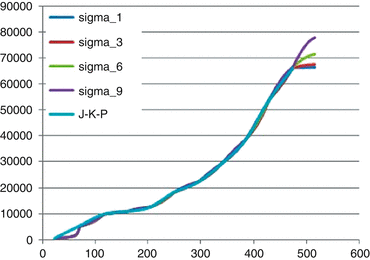

  

  Infospace. Interpolation σ ^b(x) on the compact domain

• (iii) We obtained in (ii) estimations on a fixed grid containing M = 11 points, and we now construct a function σ ^b(x) on the finite domain (see Fig. 12) which perfectly interpolates those points. Here the RKHS used is ${H}^{1}(\mathcal{D})$ where $\mathcal{D} = [\min S,\max S]$ together with the reproducing kernels $K_{1,\tau }^{\mathcal{D}}$, where τ takes the values 1, 3, 6 and 9. The functions obtained using these different reproducing kernels provide the same quality of fit within $\mathcal{D}$ and we can use any of the four outputs as the interpolated function, σ ^b, over the finite interval $\mathcal{D}$.

• (iv) Finally we optimize over m and find the RKHSH _2, m that allows the best interpolation of the M = 11 estimated points and such that the extrapolated function $\overline{\sigma }(x)$ remains as close as possible to σ ^b(x) on the third right side of $\mathcal{D}$. Of course, the reproducing kernels used in order to construct the functions σ _m and minimize the target error as in (153) are $q_{2,m}^{\mathit{RP}}$. We obtain $\overline{m} = 6.17$ (i.e. $\alpha = \frac{\overline{m}+1} {2} = 3.58$) and we can conclude that there is a bubble.

Remark 46.

One might expect $\alpha \approx 1.8$ as suggested by the green curve in Fig. 13. But this is different from what the RKHS extrapolation has selected. Why? In Fig. 13, we plot the RKHS extrapolation obtained when α = 1. 8. We have proved that

$$\displaystyle{\lim _{x\rightarrow \infty }\frac{{x}^{m+1}} {{\overline{\sigma }}^{2}(x)} = 4B(m + 1,2)\sum _{i=1}^{M}c_{ i}.}$$

The numerical computations give: $\overline{\sigma }(x) \approx \frac{{x}^{3.58}} {127009}$ when using optimization over m and $\overline{\sigma }(x) \approx \frac{{x}^{1.8}} {5.66}$ when fixing α = 1. 8. Independent of the power chosen, the c _i ’s and hence the constant of proportionality are automatically adjusted to interpolate the input points. But, as can be seen in Fig. 14, the power 3.58 is more consistent in terms of extending “naturally” the behavior of σ ^b(x) to ${\mathbb{R}}^{+}$.

Fig. 13

Infospace. Final estimator and RKHS extrapolation

Fig. 14

Infospace

Fig. 15

Geocities Stock Prices during the alleged Dotcom Bubble

Geocities: Our methodology shows that this stock did not have a price bubble. The stock prices are graphed in Fig. 15.

This is an example where we can stop at step (iii) of Procedure 43: we do not need to use RKHS theory to extrapolate our estimator in order to determine its asymptotic behavior. As seen from Fig. 16, the volatility is a nice bounded function, and any natural extension of this behavior implies the divergence of the integral $\int _{\epsilon }^{\infty }{ \frac{x} {\sigma }^{2}(x)}\mathit{dx}$. Hence the price process is a true martingale.

Fig. 16

Geocities. Estimates of σ

10.4.3 More Recent Examples

10.4.4 The Case of the IPO of LinkedIn

After giving talks based on the results of [78] with the examples of the dot com era, colleagues asked for examples from more recent and timely stocks. One of the times this occurred, at a conference in Ascona, Switzerland, May 23–27, 2011, we happened to read a New York Times article by Julie Creswell [32] discussing whether or not in the aftermath of the LinkedIn IPO the stock price had a bubble. Inspired by this controversy we obtained stock price tick data from Bloomberg.²⁶ And, we used our methodology to test whether LinkedIns stock price is exhibiting a bubble. We found, definitively, that there was indeed a price bubble in the opening days of the stock.

To perform our test, we obtained minute by minute stock price tick data for the 4 business days 5/19/2011 to 5/24/2011 from Bloomberg. There are exactly 1,535 price observations in this data set. The time series plot of LinkedIn’s stock price is contained in Fig. 17. The prices used are the open prices of each minute but the results are not sensitive to using open, high or lowest minute prices instead.

Fig. 17

LinkedIn Stock Prices from 5/19/2011 to 5/24/2011. (The observation interval is 1 min)

The maximum stock price attained by LinkedIn during this period is $120.74 and the minimum price was $81.24. As evidenced in this diagram, LinkedIn experienced a dramatic price rise in its early trading. This suggests an unusually large stock price volatility over this short time period and perhaps a price bubble.

Let us recall from our treatment of the dot com bubbles that we just treated previously in this section, that our bubble testing methodology first requires us to estimate the volatility function σ using local time based non-parametric estimators. We use two such estimators. We compare the estimation results obtained using both Florens–Zmirou’s²⁷ estimator (see Theorems 44 and 45) and the estimator developed in [78]. The implementation of these estimators requires a grid step h _n tending to zero, such that nh _n  → ∞ and $\mathit{nh}_{n}^{4} \rightarrow 0$ for the former estimator, and $\mathit{nh}_{n}^{2} \rightarrow \infty$ for the later one. We choose the step size $h_{n} = \frac{1} {{n}^{\frac{1} {3} }}$ so that all of these conditions are simultaneously satisfied. This implies a grid of seven points. The statistics are displayed in Fig. 18.

Fig. 18

Non-parametric volatility estimates

Since the neighborhoods of the grid points $118.915 and $125.764 are either not visited or visited only once, we do not have reliable estimates at these points. Therefore, we restrict ourselves to the grid containing only the first five points. We note that the last point in the new grid $112.065 still has only been visited very few times.

When using Zmirou’s estimator, confidence intervals are provided. The confidence intervals are quite wide. Given these observations, we apply our methodology twice. In the first test, we use a five point grid. In the second test, we remove the fifth point where the estimation is uncertain and we use a four point grid instead. The graph in Fig. 19 plots the estimated volatilities for the grid points together with the confidence intervals.

Fig. 19

Non parametric volatility estimation results

The next step in our procedure is to interpolate the shape of the volatility function between these grid points. We use the estimations from our non parametric estimator with the five point grid case. For the volatility time scale, we let the 4 day time interval correspond to one unit of time. This scaling does not affect the conclusions of this paper. When interpolating one can use any reasonable method. We use both cubic splines and reproducing kernel Hilbert spaces as suggested in [78], Sect. 5.2.3 item (ii). The interpolated functions are in Fig. 20.

Fig. 20

Interpolated volatility using cubic splines and the RKHS theory

From these,we select the kernel function K _1, τ as defined in Lemma 10 in [78], and we choose the parameter τ = 6.

The next step is to extrapolate the interpolated function σ ^b using the RKHS theory to the left and right stock price tails. Here we refer the reader to our treatment given in Sect. 10.1, and do not repeat the necessities here. The reader desiring a detailed treatment for this specific example is referred to the published article [79]. We mention only that we take $f(x) ={ \frac{1} {\sigma }^{2}(x)}$ and define the Hilbert space

$$\displaystyle{ H_{n} = H_{n}\big([0,\infty [\big) =\big\{ f \in {C}^{n}\big([0,\infty [\big)\mid \lim _{ x\rightarrow \infty }{x}^{k}{f}^{(k)}(x) = 0\text{ for all }0 \leq k \leq n - 1\big\} }$$

where n is the assumed degree of smoothness of f.

For n ∈ { 1, 2} fixed, we construct our extrapolation σ = σ _m as in [78], 5.2.3 item (iv), by choosing the asymptotic weighting function parameter m such that $f_{m} = \frac{1} {\sigma _{m}^{2}}$ is in H _n, m , σ _m exactly matches the points obtained from the non parametric estimation, and σ _m is as close (in norm 2) to σ ^b on the last third of the bounded interval where σ ^b is defined. Because of the observed kink and the obvious change in the rate of increase of σ ^b at the forth point, we choose n = 1 in our numerical procedure. The result is shown in Fig. 21.

Fig. 21

RKHS based extrapolation of σ ^b

We obtain m = 9. 42.

From Proposition 3 in [78], the asymptotic behavior of σ is given by

$$\displaystyle{ \lim _{x\rightarrow \infty }{x}^{m+1}f(x) = {n}^{2}B(m + 1,n)\sum _{ i=1}^{M}c_{ i} }$$

where M = 5 is the number of observations available, B is the Beta function, and the coefficients $(c_{i})_{1\leq i\leq M}$ are obtained by solving the system

$$\displaystyle{ \sum _{i=1}^{M}c_{ i}q_{n,m}^{RP}(x_{ i},x_{k}) = f(x_{k})\text{ for all }1 \leq k \leq M }$$

where $(x_{i})_{1\leq i\leq M}$ is the grid of the non parametric estimation, $f(x_{k}) ={ \frac{1} {\sigma }^{2}(x_{k})}$ and σ(x _k ) is the value at the grid point x _k obtained from the non-parametric estimation procedure. This implies that σ is asymptotically equivalent to a function proportional to x ^α with $\alpha = \frac{1+m} {2}$, that is α = 5. 21. This value appears very large, but the proportionality constant is also large. The c _i ’s are automatically adjusted to exactly match the input points $(x_{i},f(x_{i}))_{1\leq i\leq M}$.

We plot below the functions with different asymptotic weighting parameters m obtained using the RKHS extrapolation method, without optimization. All the functions exactly match the non-parametrically estimated points.

The asymptotic weighting function’s parameter m = 9. 42 obtained by optimization appears in Fig. 22 to be the estimate most consistent (within all the functions, in any Hilbert Space of the form H _1, m , that exactly match the input data) with a “natural” extension of the behavior of σ ^b to ${\mathbb{R}}^{+}$. The powerα = 5. 21 implies then that LinkedIn stock price is currently exhibiting a bubble.

Fig. 22

Extrapolated volatility functions using different reproducing kernels

Since there is a large standard error for the volatility estimate at the end point $112.065, we remove this point from the grid and repeat our procedure. Also, the rate of increase of the function between the last two last points appears large, and we do not want the volatility’s behavior to follow solely from this fact. Hence, we check to see if we can conclude there is a price bubble based only on the first 4 reliable observation points. We plot in Fig. 23 the function σ ^b (in blue) and its extrapolation to ${\mathbb{R}}^{+}$, σ (in red).

Fig. 23

RKHS based Extrapolation of σ ^b

Now M = 4. With this new grid, we can assume a higher regularity n = 2 and we obtain, after optimization, m = 7. 8543. This leads to the power α = 4. 42715 for the asymptotic behavior of the volatility. Again, although this power appears to be high given the numerical values $(x_{k},f(x_{k}))_{1\leq k\leq 4}$, the coefficients $(c_{i})_{1\leq i\leq 4}$ and hence the constant of proportionality are adjusted to exactly match the input points. The extrapolated function obtained is the most consistent (within all the functions, in any H _2, m , that exactly match the input data) in terms of extending “naturally” the behavior of σ ^b to ${\mathbb{R}}^{+}$. Again, we can conclude that there is a stock price bubble.

10.4.5 The Gold Bubble: Or Not?

Our final example is for the recent increase in gold prices (see [33]). Again, we obtained gold price tick data from Bloomberg²⁸ for the period August 25, 2011 to September 1, 2011. We used per second prices giving 73,695 data points. A graph of the spot price of gold for this period is given in Fig. 24.

Fig. 24

Time series of gold spot prices

We graph our estimated local volatility function for gold prices with its 95 % confidence interval in Fig. 25. As seen in Fig. 25, the volatility function is in fact decreasing as gold prices tend to ∞. This shows that speculative trading is not causing an increase in gold prices. Hence there is no gold price bubble.

Fig. 25

Non-parametric gold price volatility estimate with 95 % confidence intervals

Of course, our test only formally applies to the time period we have investigated, and there could be a regime change before or after this period giving a new function σ which might change whether or not a bubble is occurring. If a price bubble existed before our testing period, it may not be captured by our procedure. But, this is only true to the extent that the estimated volatility function’s shape changes across the different time periods considered. Recall that our testing procedure determines the shape of the estimated volatility function for the observedasset price range. This volatility function’s shape is then extrapolated to where the price becomes unbounded.

For gold, there is no reason to believe that the shape of the volatility function would change if we looked either backwards in time or used more current price observations. To verify this hypothesis, we studied two additional time intervals: July 4, 2011 to July 12, 2011 and September 26, 2011 to October 4, 2011. For each of these time periods we repeated the same bubble detection tests. The spot prices for gold are graphed in Figs. 26 and 27, and the estimated volatility functions are contained in Figs. 28 and 29, respectively. In both cases, the functions appear to be nicely bounded, so there is no gold price bubble in either period.

Fig. 26

Time series of gold spot prices—July 4, 2011 to July 12, 2011

Fig. 27

Time series of gold spot prices—September 26, 2011 to October 4, 2011

Fig. 28

Non-parametric gold price volatility estimate with 95 % confidence intervals—July 4, 2011 to July 12, 2011

Fig. 29

Non-parametric gold price volatility estimate with 95 % confidence intervals—September 26, 2011 to October 4, 2011

Despite the speculation that gold prices are a bubble (see for example [33]), our method shows that in fact there was not one, and that the bubbly fluctuations fall within the normal bounds of trading, rather than being indicative of excessive speculation. That our method can distinguish this bubbly appearance from the reality (or lack thereof) of a bubble is precisely the point of our methodology.

But, going forward in time, the shape of an asset’s volatility function can certainly change. Speculative trading can spontaneously increase due to a changing economic environment. And, bubbles that exist at any one time, can certainly burst and disappear. Whether or not a given time period’s trading activity applies to other time periods, as discussed above, is beyond the capacity of our statistical procedure. But fortunately for us, the stability of speculative trading activity can be determined by an independent analysis of the economic environment. And, as long as the speculative trading activity is stable and unchanging which reasoned economic analysis should be able to determine, our method applies across time periods as well.

10.4.6 Summary of the Examples

Given the price process of a risky asset that follows a stochastic differential equation under the risk neutral measure of the form

$$\displaystyle{dX_{t} =\sigma (X_{t})dW_{t}}$$

where W is a standard one dimensional Brownian motion, we provide methods for estimating the volatility coefficient σ(x) at the values where it is observed. If the behavior of σ(x) is reasonable, we extend this estimator to all of $\mathbb{R}_{+}$ via the technology of Reproducing Kernel Hilbert Spaces. Having done this, we are then able to decide on the convergence or the divergence of the integral

$$\displaystyle{\int _{\epsilon }^{\infty } \frac{x} {\sigma {(x)}^{2}}dx,}$$

for any ε > 0, which in turn determines whether or not the risky price process is experiencing, or has experienced, a bubble. Unfortunately, the test does not always work, since it depends on the behavior of σ(x).

We illustrated our methodology using data from the alleged internet dot com bubble of 1998–2001, the 2011 IPO of the stock LinkedIn, and the suspected gold bubble of August, 2011. Not surprisingly, we find that all three eventualities occur: in several cases we are able to confirm the presence of a bubble; in other cases we confirm the lack of a bubble, and in one particular case we find that the test is inconclusive.

11 The Issue of the Local Martingale Approach to Bubbles

There have been three rubrics of criticism to this approach. While the three are intertwined, nevertheless they should be separated into two types: the first is a criticism of the entire approach, and the second is a criticism of our bubble detection methodology. Of course, our bubble detection technique is pointless if one does not stipulate the validity (or at least the plausibility) of our mathematical approach, so let us first address the criticisms of the entire idea of modeling bubbles with this mathematical approach.

11.1 Discrete Time and Strict Local Martingales

There are two basic criticisms of the model. The first is based on an old controversy: modeling in discrete time versus modeling in continuous time. There is a consistent attitude, especially among economists, that continuous time is rather pointless, and needlessly complicates and obscures ideas that are relatively straightforward in discrete time; and besides, for implementation of continuous time models, often at some point one needs to discretize in any event. This idea is derived from the common belief that in economic theory both discrete and continuous time models are equivalent in the sense that one can always be used to approximate the other, or equivalently, any economic phenomena present in one is also present in the other.

One can indeed model stock prices, for example, as a discrete time series by looking (for example) at close of day data, but if one wants to model tick data, the data does not arrive in uniformly spaced time increments, and it seems more natural to view tick data as a frequently sampled collection of observations from an underlying continuous process. The sampling times are then stopping times in such a model. Of course a really fine analysis shows that even this interpretation might be naïve due to the presence of microstructure noise, and/or rounding errors (see for example [1, 77, 155], three of many recent papers on the subject). But while this approach might be naïve in this broader context, the noise does in invalidate it, but rather adds new layers of complexity.

Nevertheless some scholars have an issue with bubbles being the nuanced difference between a strict local martingale and a true martingale. In discrete time, it is widely believed that there are no strict local martingales; that all local martingales are actually true martingales. Technically this is not true (see [75, 95]) but “morally” it is in fact true, because the standard definition of conditional expectation requires an L ¹ condition, and as a consequence local martingales in the traditional sense are actually true martingales. This was shown by P.A. Meyer in 1973 [115]. To clarify, we have (from the textbook of Shiryaev [143]) the following theorem:

Theorem 47.

Let $X = (X_{n})_{n=0,1,\ldots }$ be an adapted process with X ₀ = 0. Then the following conditions are equivalent:

• X is a local martingale;

• X is a generalized martingale, i.e. $E(\vert X_{n+1}\vert \vert \mathcal{F}_{n}) < \infty ,E(X_{n+1}\vert \mathcal{F}_{n}) = X_{n}$ for all $n = 0,1,2,\ldots$

The condition that X ₀ = 0 in Theorem 47 is important: the theorem is no longer true if $X_{0}\not\in {L}^{1}$. However this characterization of discrete-time local martingales holds in the case when X is nonnegative and X ₀ is integrable. We have then the corollary:

Corollary 7.

A local martingale $X = (X_{n})_{n=0,1,\ldots ,T}$ with $X_{0} \in {L}^{1}$ and X _T ≥ 0 is a martingale.

Since we are usually dealing with price processes that are nonnegative (certainly the case for stocks), and typically X ₀ is assumed to be non-random and hence trivially in L ¹, Corollary 7 does indeed give an equivalence between local martingales and true martingales. And since we are mostly concerned with bubbles on compact time intervals [0, T] which must be strict local martingales to exist, the critics are correct that such a subtle distinction is meaningless in discrete time. Where this author disagrees with the critics is with the logical leap they make that this matters. Even in a subject as mundane as differential calculus, there are no continuous functions,²⁹ let alone differentiable ones, in discrete time; and try to teach the ideas of calculus using finite sums instead of integrals. So shall we discard calculus by the same reasoning? Another example of such reasoning would have us discard the normal distribution, since it cannot possibly exist in a finite, discretized world. Nevertheless, the normal distribution, and continuous functions and integrals can all be approximated as limits of discrete sums. But so can strict local martingales be approximated by discrete time processes; it is just that the discrete time processes will be true martingales, the strict local nature only occurring in the limit, just as the property of being a continuous function only occurs in the limit when approximating by discretized functions. For a more detailed discussion of this question we refer the interested reader to the recent article [86].

11.2 The Critique of Fragility of the Model

This critique comes principally from one paper of P. Guasoni and M. Rásonyi [61] which addresses the “fragility” of both the mathematical concept of No Free Lunch With Vanishing Risk, and that of the theory of mathematical bubbles presented in this paper. The basic premise is that if one has a sophisticated model of an economic phenomenon, it is by necessity of the subject only an approximation, and thus any model should be “robust” in some appropriate sense. For economics models, this makes sense at first blush, but one can stumble in the concept of robustness. The authors of [61] use the idea of the paths of an alternative model could be only ε close (on a logarithmic scale) to the originally proposed model, and yet have very different properties. The flaw in this logic (in this author’s opinion) is that the reasoning has the reverse order of one that is appropriate. Indeed, their implicit assumption is that mathematical models of economic phenomena arise simply from fitting curves to graphs of data. We would contend they are anything but that: one comes up with a model through economic and probabilistic reasoning, and then one checks later to see if it is reasonable by testing if it matches data well, for example by a goodness of fit procedure. If it does not, one tries to improve the reasoning, or call into question the hypotheses that led to the model and change them appropriately, in order to arrive at a better model. Indeed, in analogy with physics, the motion of a baseball is based on calculations involving models that include major forces (initial velocity, gravity, Newton’s laws of motion, friction with air resistance, etc.), usually ignoring minor forces such as the gravitational pull of the moon on the baseball. One then checks to see if predictions are valid and if observation is consistent with the model. One does not then invalidate the model if one can come up with another essentially arbitrary model that is “ε close” to the same trajectories, but without the physics reasoning and without some of the key properties of the original model.

The authors of [61] do have a point, however: robustness of a model is an appropriate question to ask. A more reasonable way to frame the problem would be, perhaps, that if one has a model given by an SDE of the form:

$$\displaystyle{ \frac{\mathit{dS}_{t}} {S_{t}} =\sigma (S_{t})\mathit{dB}_{t} +\mu (S_{t})dt;\quad S_{0} = x }$$

(155)

then one could approximate the coefficients with a sequence of functions σ _n , μ _n , $n = 1,2,\ldots$, such that σ _n and μ _n converge to σ and μ respectively (and in an appropriate sense), and consider the sequence of SDEs

$$\displaystyle{ \frac{\mathit{dS}_{t}^{n}} {S_{t}^{n}} =\sigma _{n}(S_{t}^{n})\mathit{dB}_{ t} +\mu _{n}(S_{t}^{n})\mathit{dt};\quad S_{ 0}^{n} = x }$$

(156)

and then as is well known, S ⁿ converges to S, so one can ask if, for some N large enough and n ≥ N, do the processes S ⁿ possess the desired properties? For NFLVR, it is clear that they do indeed possess NFLVR if S of (155) does, and if the functions σ _n , μ _n are reasonably (and not maliciously) chosen; for example one would want the solutions of (155) and (156) all to have unique, strong solutions. As far as bubbles are concerned, in the framework of (155), if the function σ satisfies the condition (142), then it is reasonable to choose approximating functions σ _n such that, at least for n ≥ N for some large N, the approximations σ _n have similar asymptotic behavior and also satisfy (142) for n ≥ N, and therefore establish the robustness of the bubble property of the model.

Of course, there are other possible interpretations of robustness. For example, one could approximate the differentials in an appropriate way, such as with Emery’s semimartingale topology, or (better) using the techniques of Kurtz and Protter [103], or alternatively those of Mémin and Slominski [113].³⁰ In this case one would have equations of the form

$$\displaystyle{ \frac{\mathit{dS}_{t}^{k}} {S_{t}^{k}} =\sigma (S_{t}^{k})\mathit{dB}_{ t}^{k} +\mu (S_{ t}^{k})\mathit{dA}_{ t}^{k};\quad S_{ 0} = x }$$

(157)

or even combine the two approximations to arrive at equations of the form

$$\displaystyle{ \frac{\mathit{dS}_{t}^{n,k}} {S_{t}^{n,k}} =\sigma _{n}(S_{t}^{n,k})\mathit{dB}_{ t}^{k} +\mu _{ n}(S_{t}^{n,k})\mathit{dA}_{ t}^{k};\quad S_{ 0} = x }$$

(158)

and again, if one were reasonable with the approximations (for example they should satisfy the condition UCV of [103]), one could preserve NFLVR (for example, one would have to choose $\mathit{dA}_{t}^{k} \ll d[{B}^{k},{B}^{k}]_{t}$ a.s. for large enough k, in the case where B ^k is a continuous local martingale), and also preserve the bubble property. We do not provide details here, because this is only tangential to the purpose of this paper.

11.3 “No Empirical Test Can Reliably Distinguish a Strict Local Martingale from a Martingale”

The title above is an actual quotation of a written report. It is true that any statistical based procedure can never produce truth, but at best only a good likelihood of a result. We assume this explains the presence of the word “reliably” in the quote above. However for the stochastic differential equations presented in Theorems 7 and 8 it certainly seems possible a priori, via the strong law of large numbers and the martingale central limit theorem, that one can identify (for example to the 95 % level) when the parameter is within the range where the solution is a true martingale, and within the range where the solution is a strict local martingale, even if nobody (to our knowledge) has yet tried to do so. (Indeed one should be able to use modern semimartingale estimation techniques such as those presented in [56] or more generally [72], especially for the cases of Theorems 7 and 8. For a treatise on more advanced techniques see [74].) Probably however the quotation above refers to the technique presented in Sect. 10. Of this technique, it would seem that the method of the estimation of the diffusion coefficient is beyond reproach; therefore the criticism is probably addressed to the extrapolation technique (and the idea of such) presented in the subsection titled “Bubble Detection.” The idea is to use the time honored method of Reproducing Kernel Hilbert Spaces (RKHS) made famous within Statistics circles by E. Parzen and more recently by G. Wahba (see for example [123, 156, 157]); however we use RKHS techniques in a new way here, in order to extrapolate the diffusion coefficient function $x\mapsto \sigma (x)$ to an interval of the form $(\hat{x}_{\text{max}},\infty )$ where $\hat{x}_{\text{max}}$ denotes the largest observed value $\hat{x}$. On the semi infinite interval $(\hat{x}_{\text{max}},\infty )$ observation data does not exist. Since our conclusion is based on this extrapolation, it is indeed beyond the usual domain of statistics, where procedures are consistent, in the sense that they converge to a limit as the procedure gets arbitrarily accurate. However since a consistent estimator is not possible here, the method proposed is at least an attempt to resolve the issue, and it is further enhanced by the fact that it seems to work, and to work well, when tested against data. We do not claim it is a definitive answer to this problem, but we do think it is an advance and represents the best possible method currently available. We eagerly await the work of others who hopefully will improve on this method, or propose alternative methods for the important problem of bubble detection.

11.4 A Brief Discussion of Some Alternative Methods

The literature, particularly the economics literature, concerning financial bubbles is vast. We make no attempt to give a survey here, although we have provided references to some key papers [19, 48, 49, 54, 55, 63, 68, 108, 112, 138, 139, 148, 154, 158], each of which in turn provides more references. Instead we limit ourselves to a discussion of proposed alternative methods for bubbles detection.

We know of four alternative methods that propose a methodology to detect financial bubbles.

The first method is that of “charges,” and is proposed in the papers of Jarrow and Madan [81], Gilles [57], and Gilles and Leroy [58]. To explain this we need the technical concept of a “price operator.” We let ν represent some fixed and constant (future) time. Let $\phi = (\Delta ,{\Xi }^{\nu })$ denote a payoff of an asset (or admissible trading strategy) where: (a) $\Delta = (\Delta _{t})_{0\leq t\leq \nu }$ is an arbitrary càdlàg nonnegative and non-decreasing semimartingale adapted to $\mathbb{F}$ which represents the asset’s cumulative dividend process, and (b) ${\Xi }^{\nu } \in \mathcal{F}_{\nu }$ is a nonnegative random variable which represents the asset’s terminal payoff at time ν. V ^π denotes the wealth process corresponding to the trading strategy π. This recalls our original framework for defining the fundamental price of an asset.

Definition 8 (Set of Super-replicated Cash Flows). 

$$\displaystyle{ {-4.0pt}\text{Let }\Phi :=\{\phi \in \Phi _{0} : \exists \pi \text{admissible},a \in \mathbb{R}_{+}\text{ such that }\Delta _{\nu } + {\Xi }^{\nu } \leq a + V _{\nu }^{\pi }\}.\quad }$$

(159)

The set $\Phi$ represents those asset cash flows that can be super-replicated by trading in the risky asset and money market account. As seen below, it is the relevant set of cash flows for our no dominance assumption. We first show that this subset of asset cash flows is a convex cone.

We start with a price function $\Lambda _{t} : \Phi \rightarrow \mathbb{R}_{+}$ that gives for each $\phi \in \Phi ,$ its time t price $\Lambda _{t}(\phi )$. Let $\Phi _{m} \subset \Phi$ represent the set of traded assets. Take as our economy $\Phi _{m} =\{ 1,S\}$. The no dominance assumption implies the following:

Theorem 48.

(Positivity and Linearity on $\Phi$ ) Let “ ≥ _t ” denote dominance at time t.

• 1. Let ${\phi }^{{\prime}},\phi \in \Phi$ . If ${\phi }^{{\prime}}\geq _{t}\phi$ for all t, then $\Lambda _{t}{(\phi }^{{\prime}}) > \Lambda _{t}(\phi )$ for all t almost surely.

• 2. Let $a,b \in \mathbb{R}_{+}$ and ${\phi }^{{\prime}},\phi \in \Phi$ . Then, $a\Lambda _{t}{(\phi }^{{\prime}}) + b\Lambda _{t}(\phi ) = \Lambda _{t}({a\phi }^{{\prime}} + b\phi )$ for all t almost surely.

The next theorem is established in [89] and shows that the local martingale characterization of market prices has a finitely additive market price operator if and only if bubbles exist.

Theorem 49.

Fix $t \in \mathbb{R}_{+}$ . The market price operator $\Lambda _{t}$ is countably additive if and only if bubbles do not exist.

The second approach is that of Caballero et al. [18]. As described by Phillips et al. [125], they use a “simple general equilibrium model without monetary factors, but with goods that may be partially securitized. Date-stamping the timeline of the origination and collapse of the various bubbles is a critical element in the validity of this sequential hypothesis.” They “put forward a sequential hypothesis concerning bubble creation and collapse that accounts for the course of the financial turmoil in the U.S. economy.”

The third approach builds on the above approach of [18], Phillips et al. [125, 126] study bubbles more in the spirit that is presented in this paper. They posit the existence of a dividend process D _t that is a martingale under certain conditions and such that it is “reflecting market conditions that generate cash flows.” They then define a fundamental process F _t by the relationship

$$\displaystyle{ F_{t} =\int _{ 0}^{\infty }\exp (-s(r_{ t+s}))E\{D_{t+s}\vert \mathcal{F}_{t}\}ds }$$

(160)

Here $(r_{t})_{t\geq 0}$ is the spot interest rate process, and r _D is an (assumed) constant growth rate for the interest rates such that one has the relationship

$$\displaystyle{ E\{D_{t+s}\vert \mathcal{F}_{t}\} =\exp (r_{D}s)D_{t} }$$

(161)

and then if r _D  = 0 one has that D is a martingale. Combining (160) and (161) one gets

$$\displaystyle{F_{t} =\int _{ 0}^{\infty }\exp (-s(r_{ t+s} - r_{D}))D_{t}ds}$$

Phillips et al. then make a key assumption on the exact structure of the spot discount rate r _t , and under this assumption F satisfies an SDE of the form

$$\displaystyle{ \mathit{dF}_{t} = (1 - {e}^{-\gamma })c_{ a}F_{t}\mathit{dt} +\sigma _{t}\mathit{dD}_{t} }$$

(162)

where γ is such that $(1 - {e}^{-\gamma })c_{a} > 0$. The solution of (162) can have an explosive drift under certain assumptions on the structure of the interest rates, as it approaches a special time t _b . When the drift explodes this way, they claim one has a bubble. They observe that “the discrete time path of $F_{t}\ldots$ is therefore propagated by an explosive autoregressive process with coefficient ρ > 1.” They explain their reasoning as follows:

The heuristic explanation of this behavior is as follows. As t ↗ t _b there is growing anticipation that the discount factor will soon increase. Under such conditions, investors anticipate the present to become more important in valuing assets. This anticipation in turn leads to an inflation of current valuations and price fundamentals F _t become explosive as this process continues.

The fourth and last approach we shall mention is that of D. Sornette and co-authors (they have written many papers on financial bubbles; here is a sample selection of a rather large armamentarium: [10, 66, 92, 132, 147]). We are concerned with their model known as the “Johansen–Ledoit–Sornette Bubble Model,” which we find to be the most mathematical, and closest to the spirit of this paper (see [132] for an exposition and discussion of this model). All quotations below are from the paper [132].

Sornette, together with his many co-authors over a long series of papers, propose that the dynamics of the price process satisfies a simple stochastic differential equation with drift and jump:

$$\displaystyle{ \frac{dp_{t}} {p_{t}} =\mu _{t}dt + dW_{t} - dj_{t} }$$

(163)

where p is the stock market price, and W is a standard Wiener process, and j is a point process with hazard rate h(t). The point process has one jump only, and it represents a market crash, and they introduce a random variable κ to denote the size of the crash. They assume that the aggregate effect of noise traders leads to a “crash hazard rate” of the form, with t _c denoting the time of the crash:

$$\displaystyle{ h(t) = B^{\prime}{(t - t_{c})}^{m-1} + C^{\prime}{(t - t_{ c})}^{m-1}\cos (\gamma \ln (t - t_{ c}) -\phi ^{\prime}) }$$

(164)

The authors interpret (164) by stating, “the cosine part of the second term in (164) takes into account the existence of possible hierarchical cascades of accelerating panic punctuating the growth of the bubble, resulting from a preexisting hierarchy in noise trader sizes and/or the interplay between market price impact inertia and nonlinear fundamental value investing.” And assuming p is a martingale under the risk neutral measure (no mention is made of local martingales) and conditional that the crash has not yet occurred, the authors obtain the relation μ(t) = κh(t), from which (using (164)) one derives a log periodic power law (LPPL):

$$\displaystyle{ \ln E(p_{t}) = A + B{(t - t_{c})}^{m} + C{(t - t_{ c})}^{m}\cos (\gamma \ln (t - t_{ c})-\phi ) }$$

(165)

where $B =\kappa B^{\prime}/m$ and $C = -\kappa C^{\prime}/\sqrt{{m}^{2 } {+\gamma }^{2}}$. This model, known as the JLS model, assumes that the parameter m is in between 0 and 1. Then a bubble exists when the crash hazard rate accelerates with time.

The JLS model claims that the price follows a “faster-than-exponential” growth rate during a bubble. For detection, the authors contend that financial crashes are preceded by bubbles with fluctuations. This leads to the claim that “both the bubble and the crash can be captured by the LPPL when specific bounds are imposed on the critical parameters m and γ.” This is elaborated upon in [10].

In a very recent paper of Hüsler, Sornette, and Hommes [70] the three authors dismiss the bubble detection technique of [78] presented in this paper, by claiming that an earlier paper by Andersen and Sornette [4] has “shown that some (and perhaps most) bubbles are not associated with an increase in volatility.” However an examination of their model (which is again a version of the JLS model) shows that the assumed extreme simplicity of their model of the evolution of a risky asset price, seems to make erroneous conclusions easy to reach.

Remark 50.

The primary difference between the two alternative methods presented above (those of Phillips et al. and of Sornette et al.), and the one presented in this article, is that both alternative approaches make assumptions (albeit very different ones) on the drifts in their models that lead to bubbles (under their [different] understandings of what constitutes a bubble), whereas in our presentation the key assumptions related to bubbles revolve around the diffusive part of the model. One sees this in (162) for Phillips et al., and for the Sornette et al. model one sees it with the inclusion of a hazard rate implicit in (163), as seen in (165). In addition, the Sornette et al. alternative model above is inextricably tied to a relatively simple and specialized Brownian paradigm. The Phillips model includes dividends in the fundamental model as well as interest rates, but excludes what we have called X _τ , a final payoff in the event of bankruptcy or dissolution for some reason, such as a merger or a payout.

References

Y. Aït-Sahalia, J. Yu, High frequency market microstructure noise estimates and liquidity measures. Ann. Appl. Stat. 3, 422–457 (2009)
K. Amin, R. Jarrow, Pricing Foreign currency options under stochastic interest rates. J. Int. Money Financ. 10(3), 310–329 (1991)
L.B.G. Andersen, V. Piterbarg, Moment explosions in stochastic volatility models. Financ. Stoch. 11, 29–50 (2007)
J.V. Andersen, D. Sornette, Fearless versus fearful speculative financial bubbles. Phys. A 337, 565–585 (2004)
N. Aronszajin, La théorie générale des noyaux reproduisants et ses applications, Première Partie. Proc. Camb. Philos. Soc. 39, 133–153 (1943)
N. Aronszajn, Theory of reproducing kernels. Trans. Am. Math. Soc. 68, 337–404 (1951)
Y. Balasko, D. Cass, K. Shell, Market participation and sunspot equilibria. Rev. Econ. Stud. 62, 491–512 (1995)
C. Baldwin, LinkedIn shares were a bubble: Academic model (2 June 2011). Available (for example) at the URL http://www.easybourse.com/bourse/international/news/918606/linkedin-shares-were-a-bubble-academic-model.html,
E. Bayraktar, C. Kardaras, H. Xing, Strict local martingale deflators and valuing American call-type options. Financ. Stoch. 16, 275–291 (2011)
K. Bastiaensen, P. Cauwels, Z.-Q. Jiang, D. Sornette, R. Woodard, W.-X. Zhou, Bubble diagnosis and prediction of the 2005–2007 and 2008–2009 Chinese stock market bubbles. J. Econ. Behav. Organ. 74, 149–162 (2010)
A. Bentata, M. Yor, Ten notes on three lectures: From Black–Scholes and Dupire formulae to last passage times of local martingales, in Notes from a Course at the Bachelier Seminar, 2008
B. Bernanke, Senate Confirmation Hearing, December 2009. This is quoted in many places; one example is Dealbook, edited by Andrew Ross Sorkin (January 6, 2010)
J. Berman, Apple not bringing overseas cash back home, Blames U.S. tax policy. The Huffington Post (March 19, 2012), online at the URL: http://www.huffingtonpost.com/2012/03/19/apple-us-tax-law_n_1362934.html
F. Biagini, H. Föllmer, S. Nedelcu, Shifting martingale measures and the slow birth of a bubble, Working paper, 2012
P. Biane, M. Yor, Quelques Précisions sur le Méandre Brownien. Bull. de la Soc. Math. 2 Sér. 112, 101–109 (1988)
M. Blais, P. Protter, An analysis of the supply curve for liquidity risk through book data. Int. J. Theor. Appl. Financ. 13(6), 821–838 (2010)
A. Bris, W.N. Goetzmann, N. Zhu, Efficiency and the bear: Short sales and markets around the world. J. Financ. 62(3), 1029–1079 (2007)
R. Caballero, E. Fahri, P.-O. Gourinchas, Financial crash, commodity prices and global imbalances. Brookings Pap. Econ. Act. Fall, 1–55 (2008)
C. Camerer, Bubbles and fads in asset prices. J. Econ. Sur. 3(1), 3–41 (1989)
R. Carmona (ed.), Indifference Pricing: Theory and Applications (Princeton University Press, Princeton, 2008)
P. Carr, T. Fisher, J. Ruf, On the hedging of options On exploding exchange rates, preprint (2012)
D. Cass, K. Shell, Do sunspots matter? J. Polit. Econ. 91(2), 193–227 (1983)
U. Çetin, R. Jarrow, P. Protter, Liquidity risk and arbitrage pricing theory. Financ. Stoch. 8, 311–341 (2004)
U. Çetin, M. Soner, N. Touzi, Option hedging for small investors under liquidity costs. Financ. Stoch. 14, 317–341 (2010)
A. Charoenrook, H. Daouk, A study of market-wide short-selling restrictions (February 2005). Available at SSRN: http://ssrn.com/abstract=687562orhttp://dx.doi.org/10.2139/ssrn.687562
J. Chen, H. Hong, J. Stein, Breadth of ownership and stock returns. J. Financ. Econ. 66, 171–205 (2002)
P. Cheridito, D. Filipovic, M. Yor, Equivalent and absolutely continuous measure changes for jump-diffusion processes. Ann. Probab. 15, 1713–1732 (2005)
R. Chernow, The House of Morgan (Atlantic Monthly Press, New York, 1990)
K.L Chung, R.J.Williams, Introduction to Stochastic Integration, 2nd edn. (Birkhäuser, Boston, 1990)
A. Cox, D. Hobson, Local martingales, bubbles and option prices. Financ. Stoc. 9, 477–492 (2005)
J. Cox, J. Ingersoll, S. Ross, The relationship between forward prices and futures prices. J. Financ. Econ. 9(4), 321–346 (1981)
J. Creswell, Analysts are Wary of LinkedIn’s stock Surge. New York Times Digest 4 (Monday, May 23, 2011)
S.M. Davidoff, How to deflate a gold bubble (that might not even exist). Dealbook; The New York Times (August 30, 2011)
F. Delbaen, W. Schachermayer, A general version of the fundamental theorem of asset pricing. Math. Ann. 300(3), 463–520 (1994)
F. Delbaen, W. Schachermayer, The fundamental theorem of asset pricing for unbounded stochastic processes. Math. Ann. 312(2), 215–250 (1998)
F. Delbaen, W. Schachermayer, A simple counter-example to several problems in the theory of asset pricing. Math. Financ. 8, 1–12 (1998)
F. Delbaen, W. Schachermayer, in The Mathematics of Arbitrage. Springer Finance (Springer, Heidelberg, 2005)
F. Delbaen, H. Shirakawa, No arbitrage condition for positive diffusion price processes. Asia Pacific Financ. Mark. 9, 159–168 (2002)
C. Dellacherie, Capacités et Processus Stochastiques (Springer, Berlin, 1972)
H. Dengler, R.A. Jarrow, Option pricing using a binomial model with random time steps (a formal model of gamma hedging). Rev. Deriv. Res. 1, 107–138 (1997)
K. Diether, C. Malloy, A. Scherbina, Differences of opinion and the cross section of stock returns. J. Financ. 52, 2113–2141 (2002)
D. Duffie, Dynamic Asset Pricing Theory, 3rd edn. (Princeton University Press, Princeton, 2001)
B. Dupire, Pricing and hedging with smiles, in Mathematics of Derivative Securities (Cambridge University Press, Cambridge, 1997), pp. 103–112
E. Ekström, J. Tysk, Convexity and the Black–Scholes equation. Ann. Appl. Probab. 19, 1369–1384 (2009)
E. Ekström, P. Lötstedt, L. Von Sydow, J. Tysk, Numerical option pricing in the presence of bubbles. Quant. Financ. 11(8), 1125–1128 (2011)
K.D. Elworthy, X.M. Li, M. Yor, The importance of strictly local martingales; applications to radial Ornstein–Uhlenbeck processes. Probab. Theory Relat. Fields 115, 325–355 (1999)
H.J. Engelbert, W. Schmidt, Strong Markov continuous local martingales and solutions of one-dimensional stochastic differential equations, Parts I, II, and III. Math. Nachr. 143, 167–184; 144, 241–281; 151, 149–197 (1989/1991)
G. Evans, A test for speculative bubbles in the sterling-dollar exchange rate: 1981–1984. Am. Econ. Rev. 76(4), 621–636 (1986)
J.D. Farmer, The economy needs agent-based modelling. Nature 460, 680–681 (2009)
R. Fernholz, I. Karatzas, Relative arbitrage in volatility stabilized markets. Ann. Financ. 1, 149–177 (2005)
Finfacts web site: http://www.finfacts.com/Private/curency/djones.htm. Accessed 2012
D. Florens-Zmirou, On estimating the diffusion coefficient from discrete observations. J. Appl. Probab. 30, 790–804 (1993)
H. Föllmer, M. Schweizer, Hedging of contingent claims under incomplete information, in Applied Stochastic Analysis, ed. by M.H.A. Davis, R.J. Elliott (Gordon and Breach, New York, 1991), pp. 389–414
K. Froot, M. Obstfeld, Intrinsic bubbles: The case of stock prices. Am. Econ. Rev. 81(5), 1189–1214 (1991)
J.K. Galbraith, A Short History of Financial Euphoria (Penguin Books, New York, 1993)
V. Genon-Catalot, J. Jacod, On the estimation of the diffusion coefficient for multi dimensional diffusion processes. Ann. de l’I.H.P B 29, 119–151 (1993)
C. Gilles, Charges as equilibrium prices and asset bubbles. J. Math. Econ. 18, 155–167 (1988)
C. Gilles, S.F. LeRoy, Bubbles and charges. Int. Econ. Rev. 33(2), 323–339 (1992)
J. Goldstein, Interview with William Dudley, the President of the New York Federal Reserve. Planet Money (April 9, 2010)
P. Grandits, T. Rheinlander, On the minimal entropy martingale measure. Ann. Probab. 30, 1003–1038 (2002)
P. Guasoni, M. Rasonyi, Fragility of arbitrage and bubbles in diffusion models, preprint (2011). Available at SSRN: http://ssrn.com/abstract=1856223orhttp://dx.doi.org/10.2139/ssrn.1856223
M. Guidolina, A. Timmermann, Asset allocation under multivariate regime switching. J. Econ. Dyn. Control 31, 3503–3544 (2007)
S. Heston, M. Loewenstein, G.A. Willard, Options and bubbles. Rev. Financ. Stud. 20(2), 359–390 (2007)
M. Hoffmann, L p Estimation of the diffusion coefficient. Bernoulli 5, 447–481 (1999)
T. Hollebeek, T.S. Ho, H. Rabitz, Constructing multidimensional molecular potential energy surfaces from AB initio data. Annu. Rev. Phys. Chem. 50, 537–570 (1999)
C.H. Hommes, A. Huesler, D. Sornette, Super-exponential bubbles in lab experiments: evidence for anchoring over-optimistic expectations on price, preprint (2012). Available at http://arxiv.org/abs/1205.0635
H. Hong, J. Scheinkman, W. Xiong, Advisors and asset prices: A model of the origins of bubbles. J. Financ. Econ. 89, 268–287 (2008)
H. Hulley, The economic plausibility of strict local martingales in financial modeling, in Contemporary Quantitative Finance, ed. by C. Chiarella, A. Novikov (Springer, Berlin, 2010)
H. Hulley, E. Platen, A visual criterion for identifying Itô diffusions as martingales or strict local martingales, in Seminar on Stochastic Analysis, Random Fields and Applications VI. Progress in Probability, vol. 63, Part 1 (2011), pp. 147–157
A. Hüsler, D. Sornette, C.H. Hommes, Super-exponential bubbles in lab experiments: evidence for anchoring over-optimistic expectations on price, Swiss Finance Institute Research Paper No. 12–20 (2012). Available at SSRN: http://ssrn.com/abstract=2060978orhttp://dx.doi.org/10.2139/ssrn.2060978
J. Jacod, Rates of convergence to the local time of a diffusion. Ann. de l’Institut Henri Poincaré Sect. B 34, 505–544 (1998)
J. Jacod, Non-parametric kernel estimation of the coefficient of a diffusion. Scand. J. Stat. 27, 83–96 (2000)
J. Jacod, P. Protter, Risk neutral compatibility with option prices. Financ. Stoch. 14, 285–315 (2010)
J. Jacod, P. Protter, Discretization of Processes (Springer, Heidelberg, 2012)
J. Jacod, A. Shiryaev, Local martingales and the fundamental asset pricing theorems in the discrete-time case. Financ. Stoch. 2, 259–273 (1998)
J. Jacod, A. Shiryaev, Limit Theorems for Stochastic Processes, 2nd edn. (Springer, Heidelberg, 2003)
J. Jacod, Y. Li, P. Mykland, M. Podolskij, M. Vetter, Microstructure noise in the continuous case: The pre-averaging approach. Stoch. Process. Their Appl. 119, 2249–2276 (2009)
R. Jarrow, Y. Kchia, P. Protter, How to detect an asset bubble. SIAM J. Financ. Math. 2, 839–865 (2011)
R. Jarrow, Y. Kchia, P. Protter, Is there a bubble in LinkedIn’s stock price? J. Portf. Manag. 38, 125–130 (2011)
R. Jarrow, Y. Kchia, P. Protter, Is gold in a bubble? Bloomberg’s Risk Newsletter 8–9 (October 26, 2011)
R. Jarrow, D. Madan, Arbitrage, martingales, and private monetary value. J. Risk 3(1), 73–90 (2000)
R. Jarrow, G. Oldfield, Forward contracts and futures contracts. J. Financ. Econ. 9(4), 373–382 (1981)
R. Jarrow, P. Protter, An introduction to financial asset pricing theory, in Handbook in Operation Research and Management Science: Financial Engineering, vol. 15, ed. by J. Birge, V. Linetsky. (North Holland, New York, 2007), pp. 13–69
R. Jarrow, P. Protter, Forward and futures prices with bubbles. Int. J. Theor. Appl. Financ. 12(7), 901–924 (2009)
R. Jarrow, P. Protter, Foreign currency bubbles. Rev. Deriv. Res. 14(1), 67–83 (2011)
R. Jarrow, P. Protter, Discrete versus continuous time models: Local martingales and singular processes in asset pricing theory. Financ. Res. Lett. 9, 58–62 (2012)
R. Jarrow, Y. Yildirim, Pricing treasury inflation protected securities and related derivatives using an HJM model. J. Financ. Quant. Anal. 38(2), 337–358 (2003)
R. Jarrow, P. Protter, K. Shimbo, Asset price bubbles in a complete market, in Adv. Math. Financ. [in Honor of Dilip B. Madan], ed. by M.C. Fu, D. Madan (2006), pp. 105–130
R. Jarrow, P. Protter, K. Shimbo, Asset price bubbles in incomplete markets. Math. Financ. 20, 145–185 (2010)
R. Jarrow, P. Protter, A. Roch, A liquidity-based model for asset price bubbles. Quant. Financ. (2011). doi:10.1080/14697688.2011.620976
R. Jarrow, P. Protter, S. Pulido, The effect of trading futures on short sales constraints, preprint (2012)
A. Johansen, D. Sornette, Modeling the stock market prior to large crashes. Eur. Phys. J. B 9, 167–174 (1999)
G. Johnson, L.L. Helms, Class D supermartingales. Bull. Am. Math. Soc. 14, 59–61 (1963)
B. Jourdain, Loss of martingality in asset price models with lognormal stochastic volatility, Preprint CERMICS 2004-267 (2004). http://cermics.enpc.fr/reports/CERMICS-2004/CERMICS-2004-267.pdf
Y. Kabanov, In discrete time a local martingale is a martingale under an equivalent probability measure. Financ. Stoch. 12, 293–297 (2008)
I. Karatzas, C. Kardaras, The numéraire portfolio in semimartingale financial models. Financ. Stoch. 11, 447–493 (2007)
I. Karatzas, S. Shreve, Brownian Motion and Stochastic Calculus, 2nd edn. (Springer, New York, 1991)
I. Karatzas, S. Shreve, Methods of Mathematical Finance (Springer, New York, 2010)
C. Kardaras, Valuation and parity formulas for exchange options, preprint (2012). Available at arXiv: arXiv:1206.3220v1 [q-fin.PR]
C. Kardaras, D. Kreher, A. Nikeghbali, Strict local martingales and bubbles, preprint (2012). Available at arXiv:1108.4177v1 [math.PR]
S. Kotani, On a condition that one dimensional diffusion processes are martingales, in In Memoriam Paul-André Meyer. Séminaire de Probabilitiés XXXIX. Lecture Notes in Mathematics, vol. 1874 (2006), pp. 149–156
D. Kramkov, Discussion on how to detect an asset bubble, by R. Jarrow, Y. Kchia, and P. Protter; Remarks given after the presentation of P. Protter at the meeting, Contemporary Issues and New Directions in Quantitative Finance, Oxford, England, 10 July 2010
T.G. Kurtz, P. Protter, Weak limit theorems for stochastic integrals and stochastic differential equations. Ann. Probab. 19s, 1035–1070 (1991)
T.G. Kurtz, P. Protter, Characterizing the weak convergence of stochastic integrals, in Stochastic Analysis, ed. by M. Barlow, N. Bingham (Cambridge University Press, Cambridge, 1991), pp. 255–259
O.A. Lamont, R.H. Thaler, Can the market add and subtract? Mispricing in tech stock Carve-outs. J. Polit. Econ. 111, 227–268 (2003)
X. Li, M. Lipkin, R. Sowers, Dynamics of Bankrupt stocks, preprint (2012). Available at SSRN: http://ssrn.com/abstract=2043631
P.L. Lions, M. Musiela, Correlations and bounds for stochastic volatility models. Ann. Inst. Henri Poincaré, (C) Nonlinear Anal. 24(1), 1–16 (2007)
M. Loewenstein, G.A. Willard, Rational equilibrium asset-pricing bubbles in continuous trading models. J. Econ. Theory 91, 17–58 (2000)
H.P. McKean, Jr., Stochastic Integrals (AMS Chelsea Publishing, 2005) [Originally published in 1969 by Academic Press, New York]
D. Madan, M. Yor, Itôs integrated formula for strict local martingales, in In Memoriam Paul-André Meyer, Séminaire de Probabilités XXXIX, ed. by M. Emery, M. Yor. Lecture Notes in Mathematics, vol. 1874 (Springer, Berlin, 2006), pp. 157–170
J. Markham, A Financial History of Modern U.S. Corporate Scandals: From Enron to Reform (M.E. Sharpe, Armonk, 2005)
R. Meese, Testing for bubbles in exchange markets: A case of sparkling rates? J. Polit. Econ. 94(2), 345–373 (1986)
J. Mémin, L. Slominski, Condition UT et Stabilité en Loi des Solutions dEquations Différentielles Stochastiques, in Sém. de Proba. XXV. Lecture Notes in Mathematics, vol. 1485 (1991), pp. 162–177
R. Merton, Theory of rational option pricing. Bell J. Econ. 4(1), 141–183 (1973)
P.A. Meyer, in Martingales and Stochastic Integrals. Lecture Notes in Mathematics, vol. 284 (Springer, Berlin, 1972/1973)
A. Mijatovic, M. Urusov, On the martingale property of certain local martingales. Probab. Theory Relat. Fields 152, 1–30 (2012)
A. Mijatovic, M. Urusov, Convergence of integral functionals of one-dimensional diffusions. Probab. Theory Relat. Fields 152, 1–30 (2012)
E. Miller, Risk, uncertainty and divergence of opinion. J. Financ. 32, 1151–1168 (1977)
P. Monat, C. Stricker, Föllmer-Schweizer decomposition and mean-variance hedging for general claims. Ann. Probab. 23, 605–628 (1995)
A. Nikeghbali, An essay on the general theory of stochastic processes. Probab. Sur. 3, 345–412 (2006)
E. Ofek, M. Richardson, R.F. Whitelaw, Limited arbitrage and short sales restrictions: Evidence from the options markets. J. Financ. Econ. 74(2), 305–342 (2004)
S. Pal, P. Protter, Analysis of continuous strict local martingales via h-transforms. Stoch. Process. Their Appl. 120, 1424–1443 (2010)
E. Parzen, Statistical inference on time series by RKHS methods, in Proceedings 12th Biennial Seminar, ed. by R. Pyke. (Canadian Mathematical Congress, Montreal, 1970), pp. 1–37
C. Profeta, B. Roynette, M. Yor, Option Prices as Probabilities: A New Look at Generalized Black-Scholes Formulae (Springer, Heidelberg, 2010)
P.C.B. Phillips, J. Yu, Dating the timeline of financial bubbles during the subprime crisis. Quant. Econ. 2, 455–491 (2011)
P.C.B. Phillips, Y. Wu, J. Yu, Explosive behavior in the 1990s Nasdaq: When did exuberance escalate asset values? Int. Econ. Rev. 52, 201–226 (2011)
P. Protter, A partial introduction to financial asset pricing theory. Stoch. Process. Their Appl. 91, 169–203 (2001)
P. Protter, Stochastic Integration and Differential Equations, version 2.1, 2nd edn. (Springer, Heidelberg, 2005)
P. Protter, The financial meltdown. Gazette de la Soc. des Math. de Fr. 119, 76–82 (2009)
P. Protter, K. Shimbo, No arbitrage and general semimartingales, in Markov Processes and Related Topics: A Festschrift for Thomas G. Kurtz. IMS Lecture Notes–Monograph Series, vol. 4 (2008), pp. 267–283
S. Pulido, The fundamental theorem of asset pricing, the hedging problem and maximal claims in financial markets with short sales prohibitions. Ann. Appl. Probab., preprint (2011). Available at http://arxiv.org/abs/1012.3102 (to appear)
R. Rebib, D. Sornette, R. Woodard, W. Yan, Detection of crashes and rebounds in major equity markets. Int. J. Portf. Anal. Manag. 1(1), 59–79 (2012)
A. Roch, Liquidity risk, volatility, and financial bubbles, Ph.D. Thesis, Applied Mathematics, Cornell University, 2009. Available at the URL dspace.library.cornell.edu/bitstream/1813/.../Roch,\%20Alexandre.pdf
A. Roch, Liquidity risk, price impacts and the replication problem. Financ. Stoch. 15(3), 399–419 (2011)
A. Roch, M. Soner, Resilient price impact of trading and the cost of illiquidity (2011). Available at SSRN: http://ssrn.com/abstract=1923840orhttp://dx.doi.org/10.2139/ssrn.1923840.
L.C.G. Rogers, S. Singh, The costs of illiquidity and its effect on hedging. Math. Financ. 20(4), 597–615 (2010)
J. Ruf, Hedging under arbitrage. Math. Financ. 23, 297–317 (2013)
J. Scheinkman, W. Xiong, Overconfidence and speculative bubbles. J. Polit. Econ. 111(6), 1183–1219 (2003)
J. Scheinkman, W. Xiong, Heterogeneous beliefs, speculation and trading in financial markets, in Paris-Princeton Lecture Notes on Mathematical Finance 2003. Lecture Notes in Mathematics, vol. 1847 (2004), pp. 217–250
P. Schönbucher, A market model for stochastic implied volatility. R. Soc. Lond. Philos. Trans. Ser. A Math. Phys. Engr. Sci. 357, 2071–2092 (1999)
M. Schweizer, J. Wissel, Term structures of implied volatilities: Absence of arbitrage and existence results. Math. Financ. 18, 77–114 (2008)
M. Schweizer, J. Wissel, Arbitrage-free market models for option prices: The multi-strike case. Financ. Stoch. 12, 469–505 (2008)
A.N. Shiryaev, Probability (Springer, Heidelberg, 1984)
S. Shreve, Stochastic Calculus for Finance II: Continuous Time Models (Springer, New York, 2004)
C. Sin, Complications with stochastic volatility models. Adv. Appl. Probab. 30, 256–268 (1998)
D. Sondermann, in Introduction to Stochastic Calculus for Finance: A New Didactic Approach. Lecture Notes in Economic and Mathematical Systems (Springer, Berlin, 2006)
D. Sornette, R. Woodard, W. Yan, W-X. Zhou, Clarifications to questions and criticisms on the Johansen-Ledoit-Sornette bubble model, preprint (2011). Available at arXiv:1107.3171v1
M. Swayne, How to detect a gold bubble, in eHow Money (November 28, 2010), at the URL http://www.ehow.com/how_7415180_detect-gold-bubble.html
W.H. Taft, Present Day Problems: A Collection of Addresses Delivered on Various Occasions. (Books for Libraries Press, Freeport, 1967); Originally published in 1908
M. Taylor, Purchasing power parity. Rev. Int. Econ. 11(3), 436–452 (2003)
A. Taylor, M. Taylor, The purchasing power parity debate. J. Econ. Perspect. 18(4), fall, 135–158 (2004)
C. Thomas-Agnan, Computing a family of reproducing kernels for statistical applications. Numer. Algorithms 13, 21–32 (1996)
J. Tirole, On the possibility of speculation under rational expectations. Econometrica 50(5), 1163–1182 (1982)
J. Tirole, Asset bubbles and overlapping generations. Econometrica 53(5), 1071–1100 (1985)
V. Todorov, Estimation of continuous-time stochastic volatility models with jumps using high-frequency data. J. Econom. 148, 131–148 (2009)
G. Wahba, Spline models for observational data, in CBMS-NSF Regional Conference Series in Applied Mathematics, vol. 59 (SIAM, Philadelphia, 1990)
G. Wahba, An introduction to model building With reproducing kernel Hilbert spaces (2000). Available for free download at http://www.stat.wisc.edu/~wahba/ftp1/interf/index.html
P. Weil, On the possibility of price decreasing bubbles. Econometrica 58(6), 1467–1474 (1990)
Wikipedia page http://en.wikipedia.org/wiki/Dot-com_bubble. Last updated 29 May 2013
N. Wingfield, Flush with cash, apple plans buyback and dividend. New York Times (March 19, 2012)
WRDS, Lastminute.com, bid prices, from 14 March 2000 to 30 July 2004; WRDS, eToys, bid prices, from 20 May 1999 to 26 February 2001; WRDS, Infospace, bid prices, from 15 December 1998 to 19 September 2002; WRDS, Geocities, bid prices, from 11 August 1998 to 28 May 1999
Acknowledgements
The author wishes to thank Vicky Henderson and Ronnie Sircar for their kind invitation to do this project. He also wishes to thank Celso Brunetti, Roy DeMeo, John Hall, Jean Jacod, Robert Jarrow, Alexander Lipton, Wesley Phoa, and for helpful comments and criticisms, and his co-authors on the subject of bubbles, Younes Kchia, Soumik Pal, Sergio Pulido, Alexandre Roch, Kazuhiro Shimbo, and especially Robert Jarrow. He has also benefited from discussions with Sophia (Xiaofei) Liu, Johannes Ruf, Etienne Tanre, and especially Denis Talay. An anonymous referee gave us many useful suggestions and we thank this referee for his or her careful reading of this work. The author is grateful to the NSF for its financial support. He is also grateful for a sabbatical leave from Columbia University, and the author thanks the hospitality of the Courant Institute of NYU, and INRIA, Sophia–Antipolis, where he spent parts of his sabbatical leave.
Author information
Authors and Affiliations
Corresponding author
Rights and permissions
Copyright information
© 2013 Springer International Publishing Switzerland
About this chapter
Cite this chapter
Protter, P. (2013). A Mathematical Theory of Financial Bubbles. In: Paris-Princeton Lectures on Mathematical Finance 2013. Lecture Notes in Mathematics, vol 2081. Springer, Cham. https://doi.org/10.1007/978-3-319-00413-6_1
Download citation
DOI: https://doi.org/10.1007/978-3-319-00413-6_1
Published:
Publisher Name: Springer, Cham
Print ISBN: 978-3-319-00412-9
Online ISBN: 978-3-319-00413-6
eBook Packages: Mathematics and StatisticsMathematics and Statistics (R0)