
Abstract
Explanation services are a crucial aspect of symbolic reasoning systems but they have not been explored in detail for defeasible formalisms such as KLM. We evaluate prior work on the topic with a focus on KLM propositional logic and find that a form of defeasible explanation initially described for Rational Closure which we term weak justification can be adapted to Relevant and Lexicographic Closure as well as described in terms of intuitive properties derived from the KLM postulates. We also consider how a more general definition of defeasible explanation known as strong explanation applies to KLM and propose an algorithm that enumerates these justifications for Rational Closure.
Access provided by Autonomous University of Puebla. Download conference paper PDF
Keywords
- Knowledge representation and reasoning
- Defeasible reasoning
- KLM approach
- Rational closure
- Relevant closure
- Lexicographic closure
- Explanations
1 Introduction
Explanation services indicate to users of symbolic reasoning systems which parts of their knowledge base lead to particular conclusions. This is helpful particularly when the reasoner is giving unexpected results since it allows the user to identify the culprit knowledge base statements and thus debug their knowledge base [10]. Explanation services have also been found to improve knowledge base comprehension, particularly if the user is not familiar with the knowledge base [1], and to improve users’ confidence in the reasoning system [2]. There is also some evidence that formalisms of explanation can be theoretical tools in their own right; for example, Casini et al. [4] base their work on Relevant Closure fundamentally on classical justification, a form of classical explanation.
Although well-understood in the classical case, explanation has not yet been explored in detail for defeasible reasoning apart from some foundational work [3, 8]. Our work aims to improve our understanding of explanation for defeasible propositional logic and where relevant to provide algorithms for the practical implementation of explanation services.
There are many approaches to defeasible reasoning but a particularly compelling approach that has been studied at length in the literature [5,6,7, 13, 14] is the KLM approach suggested by Kraus, Lehmann and Magidor [11]. One of the major appeals of KLM is that it can be viewed from two different angles, each with its own advantages: either using a series of postulates asserting behaviours we intuitively expect of the defeasible reasoning formalism, or using a model-theoretic semantics perhaps not as obviously intuitive but more amenable to computation by means of reasoning algorithms. These two perspectives are linked by results in the literature [6, 9, 13]. Formalisms of defeasible entailment explored in the literatue for KLM include Rational Closure [13], Relevant Closure [4] and Lexicographic Closure [12].
Chama [8] proposes an algorithm for the evaluation of defeasible justifications for Rational Closure. We term this notion of defeasible justification weak justification and adapt this result to the cases of Relevant Closure and Lexicographic Closure. We then consider how this notion relates to strong explanation, a more general notion of defeasible explanation given by Brewka and Ulbricht [3] which has not yet been explored for KLM, and propose an algorithm for enumerating strong justifications for the case of Rational Closure using a revised definition of strong justification. Our final result characterises weak justification using properties with intuitive interpretations based on the KLM postulates.
2 Background
2.1 Classical Propositional Logic
We begin with a finite set \(\mathcal {P}=\left\{ p,q,\cdots \right\} \) of propositional atoms. The binary connectives \(\wedge ,\vee ,\rightarrow ,\leftrightarrow \) and the negation operator \(\lnot \) are defined recursively to form propositional formulas. The set of all such formulas over \(\mathcal {P}\) is the propositional language \(\mathcal {L}\). A valuation is a function \(\mathcal {P\rightarrow }\left\{ \mathrm {T},\mathrm {F}\right\} \) that assigns a truth value to each atom in \(\mathcal {P}\). We say that a formula \(\alpha \in \mathcal {L}\) is satisfied by a valuation \(\mathcal {I}\) if \(\alpha \) evaluates to true according to the usual truth-functional semantics given \(\mathcal {I}\). The valuations that satisfy a formula \(\alpha \) are referred to as models of \(\alpha \), and the set of models of \(\alpha \) is denoted \(\mathrm {Mod}\left( \alpha \right) \). By assertion, \(\top \) is a propositional formula satisfied by every valuation and \(\bot \) is a formula not satisfied by any valuation.
A classical knowledge base \(\mathcal {K}\) is a finite set of propositional formulas. A valuation is a model of \(\mathcal {K}\) if it is a model of every formula in \(\mathcal {K}\). A knowledge base \(\mathcal {K}\) entails a formula \(\alpha \), denoted \(\mathcal {K}\models \alpha \), if \(\mathrm {Mod}\left( \mathcal {K}\right) \subseteq \mathrm {Mod}\left( \alpha \right) \) and a formula \(\alpha \) entails a formula \(\beta \), denoted \(\alpha \models \beta \), if \(\mathrm {Mod}\left( \alpha \right) \subseteq \mathrm {Mod}\left( \beta \right) \). A knowledge base \(\mathcal {J}\) is a justification for an entailment \(\mathcal {K}\models \alpha \) if \(\mathcal {J}\) is a subset \(\mathcal {J}\subseteq \mathcal {K}\) such that \(\mathcal {J}\models \alpha \) and there is no proper subset \(\mathcal {J}'\subset \mathcal {J}\) such that \(\mathcal {J}'\models \alpha \). Algorithms for enumerating classical justifications have been explored in detail by Horridge [10].
2.2 KLM Defeasible Entailment
Although there are many approaches to defeasible reasoning, one approach that has been studied extensively in the literature is that proposed by Kraus, Lehmann and Magidor (KLM) [11]. This approach extends propositional logic by introducing defeasible implication  which can be viewed as the defeasible analogue of classical implication \(\rightarrow \). Defeasible implications (DI) are expressions of the form
  where \(\alpha \in \mathcal {L}, \beta \in \mathcal {L}\) and are read as ‘\(\alpha \) typically implies \(\beta \)’.
A defeasible knowledge base is then a finite set of defeasible implications and defeasible entailment  is defined as a binary relation over defeasible knowledge baes and defeasible implications so that
  reads as ‘\(\mathcal {K}\) defeasibly entails that \(\alpha \) typically implies \(\beta \)’. Note that while we assume that defeasible knowledge bases only contain defeasible implications, we can express any classical formula \(\alpha \) using the defeasible representation
  . From here on we will assume that knowledge bases are defeasible unless stated otherwise.
Lehmann and Magidor [13] propose a series of postulates that define rational defeasible entailment, where each postulate can be thought of as asserting an intuitive characteristic we expect of a sensible defeasible entailment relation (hence the name rational). In addition to this axiomatic definition, rational entailment relations have a model-theoretic semantics which we do not discuss here but which is (in some cases) described exactly by reasoning algorithms of reasonable computational complexity. These reasoning algorithms are a central focus in this paper and we introduce Rational Closure [13], the most well-known form of defeasible entailment for KLM, in these terms.
2.3 Rational Closure
Rational Closure is a rational definition for defeasible entailment proposed by Lehmann and Magidor [13]. Casini et al. [6] present an algorithm for Rational Closure with two distinct sub-phases, shown in Algorithms 1 and 2. Essentially, the algorithm works by imposing a ranking of typicality on the knowledge base. Then, if there is an inconsistency when computing entailment, the most typical information in this ranking is removed from the knowledge base. The ranking of statements is produced by BaseRank, shown in Algorithm 2. The lower the rank of a statement, the more typical it is.


As an illustration of the Rational Closure algorithm, consider the following example.
Example 1
Suppose one has the defeasible knowledge base \(\mathcal {K}\) containing the following information.
-
1.
Birds typically fly (
 )
) -
2.
Birds typically have eyes (
 )
) -
3.
Birds typically sing (
 )
) -
4.
Penguins typically do not fly (
 )
) -
5.
Penguins are birds (\(p \rightarrow b\))
-
6.
Max is a penguin (\(m \rightarrow p\))
 )
) )
) )
) )
)Consider the entailment of the statement ‘Max typically does not fly’ ( ). Using RationalClosure, BaseRank is first used to compute the ranking in Fig. 1. Then we start by considering all the ranks and check whether \(R_0 \cup R_1 \cup R_\infty \models \lnot m\). Since this holds, \(R_0\) is removed. We then check whether \(R_1 \cup R_\infty \models \lnot m\). Since this entailment does not hold, we stop removing ranks and check whether \(R_1 \cup R_\infty \models m \rightarrow \lnot f\). Since this entailment holds, RationalClosure will return true.

Base ranking of statements for Example 1
It is helpful to introduce some notation closely related to these algorithms [13]:
Definition 1
The materialisation \(\overline{\mathcal {K}}\) of a knowledge base \(\mathcal {K}\) is the classical knowledge base  .
.
Definition 2
The exceptionality sequence \({\mathcal {E}}_0^\mathcal {K},\dots ,{\mathcal {E}}_n^\mathcal {K}\) for a knowledge base \(\mathcal {K}\) is given by letting \({\mathcal {E}_0^\mathcal {K}}=\mathcal {K},\) and  for \(0\le i < n\) where n is the smallest index such that \(\mathcal {E}^\mathcal {K}_n=\mathcal {E}^\mathcal {K}_{n+1}\) according to these equations. The final element \({\mathcal {E}}_n^\mathcal {K}\) is usually denoted as \(\mathcal {E}_\infty ^\mathcal {K}\) as it is unique in that its statements are never retracted when evaluating entailment queries.
Definition 3
The base rank \(\mathrm {br}_\mathcal {K}\left( \alpha \right) \) of a formula \(\alpha \in \mathcal {L}\) is the smallest index i such that \(\overline{\mathcal {E}^\mathcal {K}_i}\models \lnot \alpha \). If there is no such i, then let \(\mathrm {br}_\mathcal {K}\left( \alpha \right) =\infty \). This is distinguished from the case of \(\mathrm {br}_\mathcal {K}\left( \alpha \right) =n\) where \(\mathcal {E}^\mathcal {K}_\infty \) is the first \(\mathcal {E}^\mathcal {K}_i\) having \(\overline{\mathcal {E}^\mathcal {K}_i}\models \lnot \alpha \).
We also introduce the following shorthand:
Definition 4
For a knowledge base \(\mathcal {K}\) and formula \(\alpha \), let \(\mathcal {E}_{\alpha }^{\mathcal {K}}=\mathcal {E}_{r}^{\mathcal {K}}\) where \(r=\mathrm {br}_{\mathcal {K}}\left( \alpha \right) \). The cases of \(r=\infty \) and \(r=n\) both correspond to \(\mathcal {E}_{\alpha }^{\mathcal {K}}=\mathcal {E}_{\infty }^{\mathcal {K}}\).
We note then that Rational Closure entailment  can alternatively be expressed as follows:
Proposition 1
For a knowledge base \(\mathcal {K}\) and an entailment query  ,
,

3 Weak Justification
One of the main works of interest here is that of Chama [8] which proposes a notion of defeasible justification for Rational Closure according to an algorithm closely connected to the Rational Closure reasoning algorithm. The insight here is that we should follow the same process to eliminate more general statements, and once we have done so, to use classical tools to reason about the knowledge base—only in this case we obtain classical justifications instead of testing for classical entailment. We refer to these justifications as weak justifications to distinguish from classical justifications and the strong justifications we discuss later. We express this result for KLM propositional logic in the following definition (see Appendix A for the corresponding algorithm):
Definition 5
A knowledge base \(\mathcal {J}\) is a weak justification for a Rational Closure entailment  if \(\overline{\mathcal {J}}\) is a classical justification for \(\overline{\mathcal {E}_{\alpha }^{\mathcal {K}}}\models \alpha \rightarrow \beta \). The set of weak justifications for
  is denoted
  .
.
3.1 Relevant Closure
Casini et al. [4] propose Relevant Closure which adapts the reasoning algorithm for Rational Closure so that we only retract the statements in a less specific rank that actually disagree with more specific statements in higher ranks with respect to the antecedent of the query. Relevant Closure is not rational; it does not obey all of the axioms of rational defeasible entailment.
For the sake of brevity, we do describe the reasoning algorithm procedurally. However, the essence of the Relevant Closure reasoning algorithm can be expressed simply using the following three definitions:
Definition 6
A knowledge base \(\mathcal {J}\) is an \(\varepsilon \)-justification for \(\left( \mathcal {K},\alpha \right) \) if \(\overline{\mathcal {J}}\) is a classical justification for \(\overline{\mathcal {K}}\models \lnot \alpha \).
Definition 7
A statement  is relevant for \(\left( \mathcal {K},\gamma \right) \) if
  is an element of some \(\varepsilon \)-justification for \(\left( \mathcal {K},\gamma \right) \). Let \(R\left( \mathcal {K},\gamma \right) \) be the set of statements in \(\mathcal {K}\) that are relevant for \(\left( \mathcal {K},\gamma \right) \) and \(R^{-}\left( \mathcal {K},\gamma \right) \) the set of statements in \(\mathcal {K}\) not relevant to \(\left( \mathcal {K},\gamma \right) \).
Definition 8
We have  if \(\overline{\mathcal {E}_{\alpha }^{\mathcal {K}}\cup R^{-}\left( \mathcal {K},\alpha \right) }\models \alpha \rightarrow \beta \).
What we have described here is Basic Relevant Closure, but Minimal Relevant Closure—the other definition of Relevant Closure entailment [4]—is based on a slightly altered version of relevance and the difference is not important for our purposes (i.e. minimal and basic relevance can be ‘swapped out’ by having \(R\left( \cdot ,\cdot \right) \) and \(R^{-}\left( \cdot ,\cdot \right) \) correspond to the form of relevance at hand).
Weak Justifications for Relevant Closure. We identify the following analogue of weak justification for the case of Relevant Closure entailment:
Definition 9
A knowledge base \(\mathcal {J}\) is a weak justification for an entailment  if \(\overline{\mathcal {J}}\) is a classical justification for \(\overline{\mathcal {E}_{\alpha }^{\mathcal {K}}\cup R^{-}\left( \mathcal {K},\alpha \right) }\).
In other words, we ensure that the statements in the knowledge base considered not relevant to the query remain under our consideration when materialising just as they are when evaluating Relevant Closure entailment queries. We give a corresponding algorithm in Appendix A by adapting \(\mathtt {WeakJustifyRC}\).
3.2 Lexicographic Closure
Lexicographic Closure is another rational definition for defeasible entailment proposed by Lehmann [12] which is more permissive than Rational Closure. Like Rational Closure, Lexicographic Closure can be defined both semantically and algorithmically; we once again present the algorithmic definition. Lexicographic Closure can be seen as a refinement of Rational Closure, where we remove single statements instead of entire levels when inconsistencies arise during the reasoning process. We utilize the algorithm presented by Morris et al. [15] for propositional logic as the algorithm for Lexicographic Closure. However, while Morris et al. refine the ranking of statements, we instead refine the removal of statements as shown in LexicographicClosure in Algorithm 3.

Essentially, instead of removing an entire level \(R_i\), this refinement weakens \(R_i\) by simultaneously considering all the ways of removing j statements from the level.
Weak Justifications for Lexicographic Closure. The refined method presented in LexicographicClosure is equivalent to considering a series of sub-knowledge bases which are derived by replacing \(R_i\) with all the possible subsets \(R_i\) of size \(m - j\), where m is the number of statements in \(R_i\). Using this approach, the final entailment holds if the classical entailment holds in all the final sub-knowledge bases. Thus to provide a weak justification for the entailment, we can compute the classical justifications in the sub-knowledge bases and present these as the final justification. However, we wish to maintain a structure that refers to which justifications are responsible for the entailment of the statement in each sub-knowledge base. We therefore present a tuple as our final weak justification, where the i’th element of the tuple is a justification for the entailment of the statement in the i’th sub-knowledge base. This allows us to refer to individual statements in our knowledge base instead of a single combined formula.
To compute these weak justifications, we first modify LexicographicClosure to create LexicographicClosureForJustifications. This modification is performed by returning the variable m, which represents the subset size used in the final entailment computation, and the variable i, which represents the lowest complete level used in the final entailment computation, as an ordered pair (i, m) along with the final entailment result. We can define an algorithm WeakJustificationsLC that then uses this information to reconstruct the appropriate sub-knowledge bases and compute the justifications for each sub-knowledge base using classical methods as was done for Rational Closure. Taking the cross product of these justifications then yields the final set of tuples, which are the weak justifications. Full details of both algorithms are given in Appendix A. We demonstrate how weak justifications are computed for Lexicographic Closure in the following example.
Example 2
Suppose one has the knowledge base in Example 1 and consider once again the entailment of the statement ‘penguins typically have eyes’ ( ). LexicographicClosureForJustifications returns true, along with (1, 2). Thus we reconstruct the sub-knowledge bases
  ,
,  and
and  . The set of all justifications for \(\mathcal {K}_1\), \(\mathcal {K}_2\) and \(\mathcal {K}_3\) are \(\mathcal {J}_1 = \{j_1, j_2\}\), \(\mathcal {J}_2 = \{j_1\}\) and \(\mathcal {J}_3 = \{j_2\}\) respectively, where:
 . Thus our weak justifications will be the elements of the cross products of these sets. For example, (\(j_1, j_1, j_2\)) will be a weak justification for the entailment.
4 Strong Justification for Rational Closure
While weak justifications present an intuitive and simple approach to defining defeasible explanation, their level of description is arguably limited: we are only presenting information as to why the final classical entailment holds and are thus disregarding the rest of the reasoning process such as the determination of the base rank. In this section, we apply an intuitively more comprehensive definition for defeasible explanation, referred to as strong explanation, proposed by Brewka and Ulbricht [3] to KLM style reasoning to produce what we refer to as strong justifications. In particular, we look at defining what constitutes a strong justification for Rational Closure and explore an algorithm for computing these strong justifications. Note that the proofs of propositions and full details for all algorithms not presented in this section are given in Appendix B.
4.1 Overview of the Approach
A strong justification is a set \(\mathcal {S}\) such that for any \(\mathcal {S}'\) with \(\mathcal {S} \subseteq \mathcal {S}' \subseteq \mathcal {K}\),  and the previous statement does not hold for any \(\mathcal {S}'' \subset \mathcal {S}\). This is essentially an extension of the definition for classical justification. The intuition here is that the strong justification contains ‘just enough’ of the statements such that the defeasible entailment always holds even if arbitrary statements from the knowledge base are added to the justification. Note that while weak justifications for Rational Closure are a subset of the knowledge base \(\mathcal {K}\) that entails the final statement—and hence always obey at least one aspect of this criterion—they are not necessarily strong justifications. As an illustration of this, consider the following example:
Example 3
Suppose one has a knowledge base \(\mathcal {K}\) containing the following information:
-
1.
If something walks, it typically does not fly (
 )
) -
2.
If something walks, it typically has legs (
 )
) -
3.
Pigeons typically fly (
 )
) -
4.
Pigeons typically walk (
 )
)
 )
) )
) )
) )
)This knowledge base has the ranking shown in Fig. 2a. Consider the entailment of the statement ‘if something is a pigeon and it walks then it typically flies’  . The weak justification for this statement is
  .
.
Now consider what happens when the statement  is added to \(\mathcal {W}\). Ranking
  yields the ranking shown in Fig. 2b. However, now when computing the entailment of
  , \(R_0 \models \lnot (p\wedge w)\) and so \(R_0\) is removed. But then \(\emptyset \models (p\wedge w) \rightarrow f\) is computed as the final entailment result, which does not hold. Thus \(\mathcal {W}\) is not a strong justification since
  does not entail our statement.

Base ranking of statements for Example 3
The issue that arises in Example 3 is that we can add statements to our set that allow us to entail the negation the antecedent \(\alpha \) off our entailed statement but not the negation of all the antecedents of our statements in our weak justification. This leads to some of the statements in our weak justification getting ‘mixed into’ lower ranks in which we can still ‘disprove’ \(\alpha \), which are then removed during the algorithm. However, we can extend \(\mathcal {W}\) to create the strong justification  . Here we ensure that the weak justification is always pushed above the ranks in which we can ‘disprove’ p, which are the ranks that contain justifications for \(\lnot p\).
4.2 Algorithm
We wish to define a procedure for extending weak justifications to form strong justifications as we did for Example 3. First we define the ranking of a set \(\mathcal {K}' \subseteq \mathcal {K}\) in \(\mathcal {K}\) to be the rank of the statement in \(\mathcal {K}'\) with the lowest ranking in \(\mathcal {K}\). For example, in Fig. 2a, the set  has rank 0 in \(\mathcal {K}\). We wish to ensure our weak justification is always ranked above the justifications for \(\lnot \alpha \), which we denote \(\mathcal {J}_{\lnot \alpha }\). We restrict ourselves to considering strong justifications for entailments where all justifications \(\mathcal {J}_{\lnot \alpha }\) and weak justifications have finite rank.
We start by considering every possible way of ranking the justifications \(\mathcal {J}_{\lnot \alpha }\) and then consider all possible ways of ranking weak justifications \(\mathcal {W}\) such that they are one rank higher than the highest ranked \(\mathcal {J}_{\lnot \alpha }\) in \(\mathcal {K}\). To do this we build up a sequences of subsets (\(K_0, K_1, \ldots , K_x\)) where:
-
1.
\(br_{K_i}(\gamma ) = i\)
-
2.
For all \(K' \subset K_i\), \(br_{K'}(\gamma ) < br_{K_i}(\gamma )\)
If a statement \(\gamma \) has rank n, that the justification for \(\lnot \gamma \) has rank \(n-1\). Thus we use the statement \(\gamma = \alpha \) for all justifications \(\mathcal {J}_{\lnot \alpha }\) and \(\gamma = \alpha \wedge \lnot \beta \) for all weak justifications \(\mathcal {W}\). We use this approach instead of defining a fixed initial set to ensure the subsets in the sequence constructed are minimal. ComputeSubsetSequences shown in Algorithm 4, with the sub-process Sequences shown in Algorithm 5, computes the appropriate sequences for weak justifications. Proposition 2 states that ComputeSubsetSequences will always compute at least one sequence for some weak justification.
Proposition 2
Let \(\mathcal {K}\) be a knowledge base and \(\gamma \) a formula. Provided \(br_\mathcal {K}(\gamma ) \ne \infty \), ComputeSubsetSequences returns at least one sequence of sets.

Note in Sequences, MinimalExtension(\(\alpha \), A, B) computes the set of all sets M where M is attained by adding the minimum number of statements from A to B so that B entails \(\alpha \) and Minimize(A, \(\alpha \)) returns true if we can remove statements from A and maintain the ranking of \(\alpha \) in A.

As a demonstration of how ComputeSubsetSequences creates a sequence, consider the following example.
Example 4
Consider the knowledge base and query in Example 3. ComputeSubsetSequences computes a single sequence (\(K_0, K_1, K_2\)) for the weak justifications, with  .
.
We define similar algorithms ComputeGeneralSubsetSequences and GeneralSequences for computing the sequences for all justifications \(\mathcal {J}_{\lnot \alpha }\). However, since we do not require these justifications to reach a certain rank, we do not need to work from E subsets. Instead statements are added from \(\overline{\mathcal {K}}\). We also return a sequence when the final set can no longer be minimally extended, instead of requiring the algorithm to iterate a fixed number of times. Proposition 3 states the soundness and completeness of ComputeSubsetSequences for computing the minimal ways of ranking a statement.
Proposition 3
Let \(\mathcal {K}\) be a knowledge base and \(\gamma \) a formula. Provided \(br_\mathcal {K}(\gamma ) \ne \infty \), ComputeGeneralSubsetSequences computes exactly \(M \subseteq \mathcal {K}\) such that for all \(M' \subset M, br_{M'}(\gamma ) < br_M(\gamma )\) i.e. M is minimal in terms of the ranking of \(\gamma \).
Given the ability to compute these sequences, we now define the formal extension of a weak justification to create a strong justification. If we choose a sequence \(S_\mathcal {W}\) for some weak justification, we can consider all sequences for justifications \(\mathcal {J}_{\lnot \alpha }\) and use \(S_\mathcal {W}\) to add the minimum number of statements to \(\mathcal {W}\) to ensure it is ranked above \(\mathcal {J}_{\lnot \alpha }\) in each subset in each sequence. We consider each sequence \(\mathcal {J}\) produced by ComputeGeneralSubsetSequences individually and compute all such minimal sets S for the sequence. To do this we define the algorithm StrongSequences. We start with S containing our weak justification and then iterate through each subset \(K_i^\mathcal {J}\) in \(\mathcal {J}\), checking whether \(K_i^\mathcal {J} \cup S \models \lnot m\) for all  . If this does not hold, we use \(K_{i+1}^\mathcal {W}\) from our weak justification sequence and consider all the ways of adding the minimum number of required statements to S so that \(K_i^\mathcal {J} \cup S \models \lnot m\) for all
  , where \(S'\) is the previous iteration of S in a similar manner to Algorithm 5. We repeat this process until we have considered all sets in the sequence. Essentially, what we have done is create all the minimal sets S that ensure that whenever \(\mathcal {J}_{\lnot \alpha }\) has rank j in our sequence, our weak justifications has at least rank \(j+1\).
We then consider all ways of taking a minimal set for each sequence and taking the union of these sets. The smallest set created in this manner is then taken as our strong justification. This full process is defined by the algorithm StrongJustification. Proposition 4 states the correctness of this algorithm.
Proposition 4
Let \(\mathcal {K}\) be a knowledge base and  a defeasible implication. Provided \(br_\mathcal {K}(\alpha ) \ne \infty \), StrongJustification returns a strong justification for the entailment
  .
.
We provide a simple demonstration of StrongJustification using our example from the introduction.
Example 5
Consider the knowledge base and query in Example 3. ComputeSubsetSequences produces the sequence in Example 4. ComputeGeneralSubsetSequences produces the single sequence \(\mathcal {J} = (K_0, K_1\)) with  . We start with
  for this sequence. We then consider whether \(K_1^\mathcal {J} \cup S \models \lnot p\). Since this does not hold, we add the statement
  to S. Since there are no more subsets in \(\mathcal {J}\), we return
  as the single minimal set and, since there are no other sequences, S is returned as our final strong justification.
4.3 Limitations for the Approach
While we have defined strong justification as an extension of weak justifications, not every weak justification can be extended to create a strong justification. As an illustration of this, consider the following example.
Example 6
Suppose one has the knowledge base \(\mathcal {K}\) shown in Fig. 3 and consider the entailment of the statement  . This entailment has two weak justifications:
-
1.

-
2.


\(\mathcal {W}_1\) cannot be extended to create a strong justification. If initially \(\mathcal {S}\) = \(\mathcal {W}_1\), then to ensure  , the statements
  need to be added to \(\mathcal {S}\). Then
  . But now if
  is removed from \(\mathcal {S}\), we still have
  for all \(\mathcal {S}' \subseteq \mathcal {S} \subseteq \mathcal {K}\). Thus due to the minimality property of strong justifications, \(\mathcal {W}_1\) cannot be extended to create a strong justification.

Base ranking for statements in Example 6
It is also not the case that all strong justifications can be defined as an extension of a weak justification. As a demonstration of this fact, consider the following example.
Example 7
Suppose one has a knowledge base \(\mathcal {K}\) shown in Fig. 4 and consider the entailment of the statement  . This has the weak justification
  . However, consider rather
  as the base set for extension. \(\mathcal {B}\) is not a weak justification since it contains information removed during the Rational Closure algorithm. However, \(\mathcal {B}\) can be extended to form the strong justification

First notice  . Now consider what happens if any statements are added to \(\mathcal {S}\). If we add any statements that cause \(\mathcal {B}\) to be thrown away, namely
  , the set then contains \(\mathcal {W}\) and so the entailment still holds.

Base ranking of statements for Example 7
5 Properties of Weak Justification
Weak justification has currently only been explored in terms of reasoning algorithms (such constructions as the exceptionality sequence \(\mathcal {E}\) and base ranks) and therefore an interesting question is whether it can be characterised in a more intuitive manner. In this section, we show that for every postulate of rationality there is a corresponding property obeyed by weak justification. For the sake of simplicity, our presentation here will be limited to the case of Rational Closure and therefore we assume for this section that  refers to
  . We begin by considering a strengthening of the postulates for rationality given by Lehmann and Magidor [13]:
-
1.
Left logical equivalence (LLE). If
 and
and  then
then  .
. -
2.
Right weakening (RW). If
 and
and  then
then  .
. -
3.
And. If
 and
and  then
then  .
. -
4.
Or. If
 and
and  then
then  .
. -
5.
Reflexivity (Ref).
 .
. -
6.
Cautious Monotonicity (CM). If
 and
and  then
then  .
. -
7.
Rational Monotonicity (RM). If
 and
and  then
then 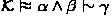 .
.
 and
and  then
then  .
. and
and  then
then  .
. and
and  then
then  .
. and
and  then
then  .
. .
. and
and  then
then  .
. and
and  then
then  .
.This is a strengthening of the KLM postulates because LLE has the condition  in favour of \(\alpha \equiv \beta \) and RW has
  in favour of \(\alpha \models \beta \). (Note here that
  is for example is a shorthand for
  as discussed in the background section.) This provides a more useful perspective for our purposes.
Our approach is to consider how defeasible justification applies to each of these axioms. Take for instance the example of And. The insight here is that if \(\alpha \) typically implies \(\beta \), and \(\alpha \) typically implies \(\gamma \), then not only should we be able to conclude that \(\alpha \) typically implies \(\beta \) and \(\gamma \), we should be able to conclude it by the same token. In this section we formalise this idea, and a similar idea for each postulate above, in relation to weak justification. The following concept helps us state these results:
Definition 10
A knowledge base \(\mathcal {D}\subseteq \mathcal {K}\) is deciding for an entailment  if \( \mathcal {D}\subseteq \mathcal {E}_{\alpha }^{\mathcal {K}}\text { and }\overline{\mathcal {D}}\models \alpha \rightarrow \beta . \)
For a given entailment, any deciding knowledge base is always a superset of a weak justification and all weak justifications are deciding (refer to Definition 5). We also have the following results for deciding knowledge bases:
Proposition 5
If \(\mathcal {D}\) is a deciding knowledge base for an entailment  and \(\mathrm {br}_{\mathcal {K}}\left( \alpha \right) \ne \infty \), then
  .
.
Proposition 6
If \(\mathcal {D}\) is a deciding knowledge base for an entailment  and we have
  , then
Proofs for these results, as well as all results in this section, are given in Appendix C. We can now state a result corresponding to each axiom of rational defeasible entailment:
Theorem 1
For any knowledge bases \(\mathcal {K},\mathcal {J}_{1},\mathcal {J}_{2}\),
- (LLE):
-
if \(\mathcal {J}_{1}\in \mathcal {J}_{W}\left( \mathcal {K},\alpha \leftrightarrow \beta \right) \) and
 , \(\mathcal {J}_{1}\cup \mathcal {J}_{2}\) is deciding for
  ;
; - (RW):
-
if \(\mathcal {J}_{1}\in \mathcal {J}_{W}\left( \mathcal {K},\alpha \rightarrow \beta \right) \) and
 , \(\mathcal {J}_{1}\cup \mathcal {J}_{2}\) is deciding for
  ;
; - (And):
-
if
 and
and 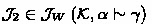 , \(\mathcal {J}_{1}\cup \mathcal {J}_{2}\) is deciding for
  ;
; - (Or):
-
if
 and
and  , \(\mathcal {J}_{1}\cup \mathcal {J}_{2}\) is deciding for
  .
. - (Ref):
-
 .
. - (CM):
-
if
 and
and  , every
  is deciding for
  ;
; - (RM):
-
if
 and
and  , every
  is deciding for
  .
.
 ,
,  ;
; ,
,  ;
; and
and  ,
,  ;
; and
and  ,
,  .
. .
. and
and  , every
  is deciding for
  ;
; and
and  , every
  is deciding for
  .
.6 Conclusions and Future Work
We have extended the principle of weak justification, previously only explored for Rational Closure, to the case of Relevant and Lexicographic Closure and proposed algorithms for enumerating these justifications. We then evaluated a revised definition of strong justification in light of certain issues and proposed an algorithm that enumerates these justifications for Rational Closure. This is, to our knowledge, the first application of strong explanation to KLM and may offer an alternative to weak justification that is perhaps more comprehensive as far as the resulting justifications are concerned. Our final result is a characterisation of weak justification in relation to the KLM postulates for rationality. This provides evidence that weak justification is a sound and generalisable notion of justification for KLM-style defeasible entailment and illustrates similarities between weak justification for the defeasible case and classical justification for the classical case.
Since the algorithm we propose for enumerating strong justifications and the declarative characterisation of weak justification were limited to the case of Rational Closure, further work might seek to apply this result to other notions of defeasible entailment for KLM or perhaps generally to rational defeasible entailment. Another possibility is to consider how these ideas apply to KLM description logic [5, 7, 14].
References
Bail. S.P.: The justificatory structure of OWL ontologies. PhD thesis, University of Manchester (2013)
Biran, O., Cotton, C.: Explanation and justification in machine learning: a survey. In: IJCAI-17 Workshop on Explainable AI (XAI), vol. 8, pp. 8–13 (2017)
Brewka, G., Ulbricht, M.: Strong explanations for nonmonotonic reasoning. In: Description Logic, Theory Combination, and All That, pages 135–146. Springer, Cham (2019). https://doi.org/10.1007/978-3-030-22102-7
Casini, G., Meyer, T., Moodley, K., Nortjé, R.: Relevant closure: a new form of defeasible reasoning for description logics. In: Fermé, E., Leite, J. (eds.), Logics in Artificial Intelligence, pp. 92–106. Springer, Cham (2021)
Casini, G., Meyer, T., Moodley, K., Varzinczak, I.: Towards practical defeasible reasoning for description logics (2013)
Casini, G., Meyer, T., Varzinczak, I.: Taking defeasible entailment beyond rational closure. In: Calimeri, F., Leone, N., Manna, M. (eds.) JELIA 2019. LNCS (LNAI), vol. 11468, pp. 182–197. Springer, Cham (2019). https://doi.org/10.1007/978-3-030-19570-0_12
Casini, G., Straccia, U.: Defeasible inheritance-based description logics. J. Artif. Intell. Res. 48, 415–473 (2013)
Chama, V.: Explanation for defeasible entailment. Master’s thesis, Faculty of Science (2020)
From propositional logic to description logics: Laura Giordano, Valentina Gliozzi, Nicola Olivetti, and Gian Luca Pozzato. semantic characterization of rational closure. Artif. Intell. 226, 1–33 (2015)
Horridge, M.: Justification based explanation in ontologies. The University of Manchester (United Kingdom) (2011)
Kraus, S., Lehmann, D., Magidor, M.: Nonmonotonic reasoning, preferential models and cumulative logics. Artif. Intell. 44(1), 167–207 (1990)
Lehmann, D.: Another perspective on default reasoning. Ann. Math. Artilf. Intell. 15(1), 61–82 (1995)
Lehmann, D., Magidor, M.: What does a conditional knowledge base entail? Artif. Intell. 55(1), 1–60 (1992)
Moodley, K.: Practical reasoning for defeasable description logics. PhD thesis, University of KwaZulu-Natal (2016)
Morris, M., Ross, T., Meyer, T.: Algorithmic definitions for KLM-style defeasible disjunctive datalog. South Afr. Comput. J. 32(2), 141–160 (2020)
Author information
Authors and Affiliations
Editor information
Editors and Affiliations
A Supplementary Material
A Supplementary Material
The full paper with the appendix containing proofs for all propositions and additional details for algorithms is available at: https://www.cair.org.za/sites/default/files/2021-11/Explanation_For_KLM.pdf
Rights and permissions
Copyright information
© 2022 Springer Nature Switzerland AG
About this paper

Cite this paper
Everett, L., Morris, E., Meyer, T. (2022). Explanation for KLM-Style Defeasible Reasoning. In: Jembere, E., Gerber, A.J., Viriri, S., Pillay, A. (eds) Artificial Intelligence Research. SACAIR 2021. Communications in Computer and Information Science, vol 1551. Springer, Cham. https://doi.org/10.1007/978-3-030-95070-5_13
Download citation
DOI: https://doi.org/10.1007/978-3-030-95070-5_13
Published:
Publisher Name: Springer, Cham
Print ISBN: 978-3-030-95069-9
Online ISBN: 978-3-030-95070-5
eBook Packages: Computer ScienceComputer Science (R0)