Defeasible Justification Using the KLM Framework

Abstract

The Kraus, Lehmann and Magidor (KLM) framework is an extension of Propositional Logic (PL) that can perform defeasible reasoning. The results of defeasible reasoning using the KLM framework are often challenging to understand. Therefore, one needs a framework within which it is possible to provide justifications for conclusions drawn from defeasible reasoning. This paper proposes a theoretical framework for defeasible justification in PL and a software tool that implements the framework. The theoretical framework is based on an existing theoretical framework for Description Logic (DL). The defeasible justification algorithm uses the statement ranking required by the KLM-style form of defeasible entailment known as Rational Closure. Classical justifications are computed based on materialised formulas (classical counterparts of defeasible formulas). The resulting classical justifications are converted to defeasible justifications, based on the input knowledge base. We provide an initial evaluation of the framework and the software tool by testing it with a representative example.

1 Introduction

The conclusions produced by reasoning tools are often difficult to understand. Justifications for such conclusions provide users with the exact statements in the knowledge base that is used to deduce the conclusion. Currently, there exist tools that provide explanations for classical entailments [9, 10, 12]. Such a tool aids users in understanding their knowledge base and reasoning systems [4] as well as providing assistance in debugging their systems [16].

Although there are well-established tools and algorithms to compute explanations for classical reasoning, there are no such tools for defeasible reasoning. While there are many approaches to defeasible reasoning, in this paper we focus only on an approach to defeasible reasoning known as the Kraus, Lehmann and Magidor (KLM) framework [14], which is an extension of Propositional Logic (PL). Chama proposed an algorithm that computes justification for defeasible entailments in Description Logic (DL) [6]. This paper’s contribution is extended Chama’s work by converting her proposed justification algorithm for DL to PL according to the well-established notions and concepts in the KLM framework. Furthermore, we implement our defeasible justification algorithm which has not been done for the KLM framework. The implementation was tested with a representative example and the result is accurate compared to manual deductions.

2 Background

In classical reasoning with PL, the notion of interpretation and entailment is well-defined [5]. Similarly, for defeasible reasoning with the KLM framework (an extension of PL), the notion of a ranked interpretation was defined [14] and a form of defeasible entailment referred to as Rational Closure was described. Based on these notions, we define an algorithm that computes justifications for defeasible entailment.

Statements in PL are built up with a finite set $\mathcal {P}=\{ p, q, ... \}$ of propositional atoms. The binary connectives $\wedge , \vee , \rightarrow , \leftrightarrow$ and the negation operator $\lnot$ can be applied recursively to form propositional formulas. An interpretation $\mathcal {I}$ is a function that maps a propositional atom to either true or false. An interpretation satisfies a formula if the formula evaluates to true under the rules of satisfiability. The $\top$ constant in PL denotes a tautology that is always interpreted to true and the $\bot$ constant is always interpreted to false.

A knowledge base is a finite set of propositional formulas. An interpretation $\mathcal {I}$ satisfies a knowledge base $\mathcal {K}$ if $\mathcal {I}$ satisfies every formula in $\mathcal {K}$. A knowledge base $\mathcal {K}$ entails a formula $\alpha$, denoted $\mathcal {K} \vDash \alpha$, if and only if every interpretation that satisfies $\mathcal {K}$ also satisfies $\alpha$. Two propositional formulas $\alpha$ and $\beta$ are logically equivalent, denoted $\alpha \equiv \beta$, if all interpretations that satisfies $\alpha$ also satisfies $\beta$ and vice versa.

Horridge defines the notion of justification to provide explanations for classical entailments [8]. A subset of formulas $\mathcal {J}$ is a justification for the entailment $\mathcal {K} \vDash \alpha$ if $\mathcal {J} \subseteq \mathcal {K}$ such that $\mathcal {J} \vDash \alpha$ and there are no proper subset $\mathcal {J}^\prime \subset \mathcal {J}$ such that $\mathcal {J}^\prime \vDash \alpha$. Horridge defined algorithms to compute justifications for classical entailment [8].

Given a knowledge base $\mathcal {K}$ and an entailed formula $\eta$, Horridge identifies all justifications for the entailment by first identifying a single justification (Algorithm 3). A justification for the entailment can be identified by first expanding a subset $\mathcal {S} \subseteq \mathcal {K}$ until $\mathcal {S} \vDash \eta$ (Algorithm 1) then contract $\mathcal {S}$ without breaking the entailment (Algorithm 2). The justification can be used as the root node in the Hitting Set Tree [17] to identify all justification for the given entailment (Algorithm 4). In this paper, the implementation of the Hitting Set Tree is based on Reiter’s algorithm.

Note that Algorithms 1, 2, 3 and 4 are slight adjusted and renamed to suit the context of this paper because Horridge’s work is done in the context of DL and Ontologies. These algorithms are used as sub-routines to construct a defeasible justification algorithm.

There are many approaches to defeasible reasoning. One of the most explored approaches in the literature is the KLM framework suggested by Kraus, Lehmann and Magidor [14]. The KLM framework extends PL by an additional binary connective known as defeasible implication, denoted by $\mathrel | \! \sim$. Defeasible implications are expressed in the form $\alpha \mathrel | \! \sim \beta$ where $\alpha$ and $\beta$ are propositional formulas. One reads $\alpha \mathrel | \! \sim \beta$ as “$\alpha$ typically implies $\beta$”. Note that $\mathrel | \! \sim$ cannot be nested.

A defeasible knowledge base is a finite set of defeasible implications. It is easily shown that a classical formula $\alpha$ is logically equivalent to the defeasible implication $\lnot \alpha \mathrel | \! \sim \, \bot$ [11]. Therefore, any knowledge base that contains classical formulas can be converted into a defeasible knowledge base. From here on we assume knowledge bases are defeasible unless stated otherwise explicitly. The material counter-part of a defeasible implication $\alpha \mathrel | \! \sim \beta$ is the classical implication $\alpha \rightarrow \beta$. The material counter-part of the knowledge base $\mathcal {K}$, denoted $\overrightarrow{\mathcal {K}}$, is the knowledge base with each of the defeasible implications in $\mathcal {K}$ replaced with its material count-part.

Similar to classical entailment, defeasible entailment, denoted $\mid \!\approx$, is a binary relation over a defeasible knowledge base and a defeasible implication. One reads $\mathcal {K} \mid \!\approx \alpha \mathrel | \! \sim \beta$ as “$\mathcal {K}$ defeasibly entails that $\alpha$ typically implies $\beta$”.

Lehmann and Magidor suggest the notion of Rational Closure as a form of defeasible entailment and presented an algorithm for Rational Closure [15]. We use the Rational Closure algorithm as a sub-routine to construct a defeasible justification algorithm. The first procedure in the rational closure algorithm is to assign rankings to formulas in the knowledge base. Low ranks are assigned to statements that are less exceptional. The infinite rank is assigned to classical statements. The ranking algorithm is shown in Algorithm 5 [11].

Based on the ranking produced by Algorithm 5, the Rational Closure algorithm removed the ranking in ascending order until the remaining formulas entail the negation of the query’s antecedent. The knowledge base defeasibly entails the query (the query is in the Rational Closure of the knowledge base) if the (materialised versions of the) remaining formulas classically entail the materialised query. Algorithm 6 is an algorithm for Rational Closure suggested by Kaliski [11].

3 Defeasible Justification Algorithm

Chama presented an algorithm that computes defeasible justification in DL [6]. Her algorithm is composed of two sub-algorithms, namely RationalClosureForJustifications and ComputeAllJustifications. We construct a defeasible algorithm for the KLM framework in a similar manner. The algorithm is composed of three sub-algorithms: RationalClosureForJustification, ComputeAllJustifications (for classical entailment) and Dematerialsiation. Each sub-algorithm is discussed in detail in this section.

We present Algorithm 7 as an algorithm that computes defeasible justification given a knowledge base $\mathcal {K}$ and an entailment $\eta = \alpha \mathrel | \! \sim \beta$. The algorithm first ranks the formulas as required by Rational Closure. A slightly adjusted Rational Closure algorithm compared to Algorithm 6, which returns additional parameters, is used. Such parameters include an ordered tuple indicating the ranked formulas and an integer indicating the ranks of formulas discarded to compute the Rational Closure.

In the case where no formulas were discarded in the Rational Closure computation, justifications are computed on the materialised knowledge base $\overrightarrow{\mathcal {K}}$ and query $\overrightarrow{\eta }$ using algorithms mentioned in Sect. 2. Alternatively, in the case where ranks of formulas were discarded in the Rational Closure computation, the discarded formulas are removed from $\mathcal {K}$ before identifying all justifications for the entailment.

Lastly, dematerialisation of justifications is required because results from algorithms mentioned in Sect. 2 are classical formulas. Any formulas in the set of justifications that is not in $\mathcal {K}$ needs to be dematerialised.

Algorithm 7 can be further enhanced to accept an input knowledge base that contains both classical and defeasible implications. From here on, we refer to a knowledge base with both classical and defeasible formulas as a “mixed knowledge base". As mentioned in Sect. 2, any classical formula $\alpha$ is logically equivalent to the defeasible implication $\lnot \alpha \mathrel | \! \sim \, \bot$ and as a result, we can pre-process a mixed knowledge base into a defeasible knowledge base.

Notice that when there are formulas of the form $\lnot \alpha \rightarrow \bot$ in a given knowledge base, line 5 in Algorithm 5 is $E_{i+1} :=\, \{ \lnot \alpha \rightarrow \bot \vert E_{i} \vDash \lnot ( \lnot \alpha ) \} = \{ \lnot \alpha \rightarrow \bot \vert E_{i} \vDash \alpha \}$. As a result, $\lnot \alpha \rightarrow \bot$ is always going to be in $E_{i+1}$. Eventually, when $E_{i-1} = E_{i}$ then while loop terminates with any formulas of the form $\lnot \alpha \rightarrow \bot$ in $E_{i-1}$ and line 8 assigns such formulas with the infinity rank. This phenomenon allows us to conclude that all classical formulas in a knowledge base are ranked infinity by Algorithm 5.

Furthermore, consider the knowledge base $\mathcal {K} = \{ \alpha \mathrel | \! \sim \beta , \alpha \mathrel | \! \sim \lnot \beta \}$ as input to Algorithm 5, the variables are assigned the following values:

• $E_{0} = \{ \alpha \rightarrow \beta , \alpha \rightarrow \lnot \beta \}$

• $E_{1} = \{ \alpha \rightarrow \beta , \alpha \rightarrow \lnot \beta \}$ because $E_{0} \vDash \lnot \alpha$.

• As a result, both $\alpha \rightarrow \beta$ and $\alpha \rightarrow \lnot \beta$ is ranked infinity.

Therefore, we can conclude that when there is a formula of the format $\alpha \mathrel | \! \sim \beta$ and another formula of the form $\alpha \mathrel | \! \sim \lnot \beta$ in the input knowledge base then both formulas are ranked infinity by Algorithm 5.

Therefore, Algorithm 5 and consequently Algorithm 7 can be enhanced to accept a mixed knowledge base as input. Algorithm 8 is a BaseRank algorithm that accepts a mixed knowledge base.

The Rational Closure algorithm for justification has the same procedures as Algorithm 6 with additional return values. Algorithm 9 is the adjusted algorithm that returns an ordered tuple of ranked formulas from Algorithm 8 and an integer that indicated the ranks of formulas discarded to compute Rational Closure.

We present an example to illustrate the intuition behind Rational Closure. Consider the following scenario where birds typically fly, penguins are birds, penguins typically cannot fly, robins are birds and birds typically have wings. From the scenario, we can construct the following knowledge base $\mathcal {K} = \{ birds \mathrel | \! \sim fly, penguins \rightarrow birds, penguins \mathrel | \! \sim \lnot fly, robins \rightarrow birds, birds \mathrel | \! \sim wings \}$.

Firstly, we use Algorithm 8 to assign a ranking to each formula in $\mathcal {K}$.

• 1. Line 1 of the algorithm extracts all classical formulas from $\mathcal {K}$ and we get the following: $\mathcal {C} = \{ penguins \rightarrow birds, robins \rightarrow birds \}$

• 2. The remaining formulas in $\mathcal {K}$ are collected into $E_{0}$. Therefore, $E_{0} = \{ birds \mathrel | \! \sim fly, penguins \mathrel | \! \sim \lnot fly, birds \mathrel | \! \sim wings \}$.

• 3. The algorithm iterates over the while loop from lines 4 to 8 until $E_{i-1} = E_{i}$. Over the iterations, we get the following values for each variable.

  • (a) $E_{1} = \{ \alpha \mathrel | \! \sim \beta \vert E_{0} \vDash \lnot \alpha \} = \{ penguins \mathrel | \! \sim \lnot fly \}$

  • (b) $R_{0} = \{ birds \mathrel | \! \sim fly, birds \mathrel | \! \sim wings \}$

  • (c) $E_{2} = \emptyset$

  • (d) $R_{1} = \{ penguins \mathrel | \! \sim \lnot fly \}$

  • (e) $E_{3} = \emptyset$

• 4. Line 9 of the algorithm assigns $R_{\infty }\, =\, \mathcal {C} \,\cup \, E_{2} \,=\, \{ penguins\, \rightarrow \,birds, robins \,\rightarrow \, birds \}$.

The final rankings of the formulas are shown in Table 1.

For querying whether robins have wings, we construct the defeasible implication $robins \mathrel | \! \sim wings$. Using the above ranking and Algorithm 9, we can compute if $\mathcal {K} \mid \!\approx robins \mathrel | \! \sim wings$. The procedures of Algorithm 9 are as follows:

• 1. Line 3 of the algorithm assigns $R = \{ penguins \mathrel | \! \sim \lnot fly, birds \mathrel | \! \sim fly, birds \mathrel | \! \sim wings \}$

• 2. Since $R_{\infty } \,\cup \, \overrightarrow{R} \,\models \, \lnot robins$ does not hold, the algorithm skips over the while loop from lines 4 to 7.

• 3. Since $R_{\infty } \cup \overrightarrow{R} \models robins \rightarrow wings$, we can conclude that $\mathcal {K} \mid \!\approx robins \mathrel | \! \sim wings$.

For querying whether penguins have wings, we construct the defeasible implication $penguins \mathrel | \! \sim wings$. The procedures of Algorithm 9 are as follows:

• 1. On line 3, we have $R = \{ penguins \mathrel | \! \sim \lnot fly, birds \mathrel | \! \sim fly, birds \mathrel | \! \sim wings \}$.

• 2. $R_{\infty } \cup \overrightarrow{R} \models \lnot penguins$ and $R \not =\emptyset$, then $R_{0}$ is removed from R and we get $R = \{ penguins \mathrel | \! \sim \lnot fly \}$

• 3. Now, $R_{\infty }~ \cup ~ \overrightarrow{R}~ \models ~ \lnot penguins$ does not hold. Therefore, the while loop terminates.

• 4. But $R_{\infty } \cup \overrightarrow{R}~ \not \models ~ penguins \rightarrow wings$, and as a result $\mathcal {K} {{\mid \!\approx \!\!\!\!{/}}}\, penguins \mathrel | \! \sim wings$.

Table 1. Ranking of formulas in $\mathcal {K}$

The defeasible justification algorithm utilises the classical justification algorithms mentioned in Sect. 2. As expected, the resulting justifications contain only classical formulas and cannot be used directly as the justifications for the defeasible entailment. Algorithm 10 takes a set of $\infty$-ranked formulas and a set of justifications as inputs. Any formulas in the justifications that are not assigned the infinity rank need to be replaced with their material counterpart.

Again, we illustrate the intuition behind defeasible justification via a representative example. Consider the following knowledge base $\mathcal {K} = \{ penguins \,\rightarrow \, birds, robins \,\rightarrow \, birds, special penguins \,\rightarrow \, penguins, birds \mathrel | \!\sim ~ fly, birds \mathrel | \! \sim ~ wings, penguins \mathrel | \! \sim ~ \lnot fly, special penguins \mathrel | \! \sim ~ fly \}$. We use the following 3 queries to demonstrate various cases the algorithm considers:

• 1. $robins \mathrel | \! \sim wings$

• 2. $penguins \mathrel | \! \sim wings$

• 3. $special penguins \mathrel | \! \sim fly$.

Firstly, Table 2 shows the formula ranking which Algorithm 8 computes.

Table 2. Ranking of formulas in $\mathcal {K}$

For query $\eta = robins \mathrel | \! \sim wings$ the defeasible justification algorithm executes as follows:

• 1. Rational Closure:

  • (a) $\overrightarrow{R} \,=\, \{ special penguins \,\rightarrow \, fly, penguins \,\rightarrow \, \lnot fly, birds \,\rightarrow \, fly, birds \,\rightarrow \, wings \}$ and $R_{\infty } \,\cup \, \overrightarrow{R} \,\models \, \lnot robins$ does not hold. Therefore, no formulas are discarded.

  • (b) Since, $R_{\infty } \,\cup \, \overrightarrow{R} \,\models \, robins \rightarrow wings$, we have $\mathcal {K} \mid \!\approx robins \mathrel | \! \sim wings$.

• 2. Since no formulas were discarded in the previous step, the entire knowledge base is used to compute the justification.

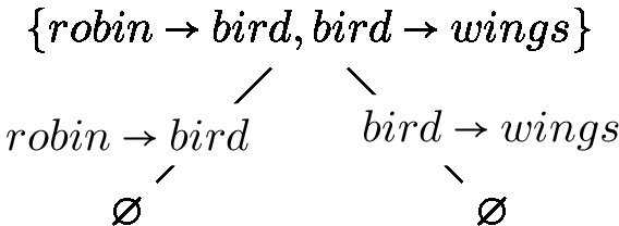
• 3. The classical justification for the entailment $\mathcal {K} \models robins \rightarrow wings$ is computed using Algorithms 4 and the following Hitting Set Tree is returned:

  

• 4. The only justification for the classical entailment $\overrightarrow{\mathcal {K}} \models robins \rightarrow wings$ is $\{robins \rightarrow birds, birds \rightarrow wings\}$.

• 5. Since the classical formula $birds \rightarrow wings$ is not in $R_{\infty }$, Algorithm 10 replaces it with the defeasible implication $birds \mathrel | \! \sim wings$.

• 6. The final justification for the defeasible entailment $\mathcal {K} \mathrel | \! \approx ~ robins \mathrel | \! \sim ~ wings$ is $\{ robins \rightarrow birds, birds \mathrel | \! \sim wings \}$.

For query $\eta \,=\, penguins \mathrel | \! \sim wings$ the defeasible justification algorithm executes as follows:

• 1. Rational Closure:

  • (a) $\overrightarrow{R} \,=\, \{ special penguins \,\rightarrow \, fly, penguins \,\rightarrow \, \lnot fly, birds \,\rightarrow \, fly, birds \,\rightarrow \, wings \}$ and $R_{\infty } \cup \overrightarrow{R} \models \lnot penguins$. Therefore, $R_{0}$ is removed from R and $R = \{ penguins \mathrel | \! \sim \lnot fly, special penguins \mathrel | \! \sim fly \}$.

  • (b) Now, $R_{\infty } \cup \overrightarrow{R} \models \lnot penguins$ does not hold.

  • (c) $R_{\infty } \cup \overrightarrow{R} \not \models \, penguins \rightarrow wings$ and therefore $\mathcal {K} {{\mid \!\approx \!\!\!\!{/}}}\, penguins \mathrel | \! \sim wings$.

• 2. The algorithm terminates with no justifications.

The final query $special penguins \mathrel | \! \sim fly$ executes as follows:

• 1. Rational Closure:

  • (a) Iterating over lines 4 to 7 of Algorithm 6, both $R_{0}$ and $R_{1}$ is removed from R such that the condition $R_{\infty } \cup \overrightarrow{R} \models \lnot \alpha$ does not hold.

  • (b) $R_{\infty } \cup \overrightarrow{R} = \{ penguins \rightarrow birds, robins \rightarrow birds, special penguins \rightarrow penguins, special penguins \rightarrow fly \} \models special penguins \rightarrow fly$.

  • (c) Hence, the defeasible entailment $\mathcal {K} \mid \!\approx special penguins \mathrel | \! \sim fly$ holds.

• 2. Classical Justification is calculated based on the remaining materialised formulas $\{ penguins \rightarrow birds, robins \rightarrow birds, special penguins \rightarrow penguins, special penguins \rightarrow fly \}$.

• 3. The following Hitting Set Tree is constructed:

  

• 4. The only justification for the classical entailment $\{ penguins \rightarrow birds, robins \rightarrow birds, special penguins \rightarrow penguins, special penguins \rightarrow fly \} \models special penguins \rightarrow fly$ is $\{special penguins \rightarrow fly \}$

• 5. Since $special penguins \rightarrow fly \not \in R_{\infty }$, Algorithm 10 replaces it with $special penguins \mathrel | \! \sim fly$.

• 6. Final defeasible justification for the defeasible entailment $\mathcal {K} \mathrel | \! \approx ~ special penguins \mathrel | \! \sim ~ fly$ is $\{\mathcal {K} \mid \!\approx special penguins \mathrel | \! \sim fly \}$.

Notice for the final query, there are two possible justifications:

• 1. $J_{1} = \{ special penguins \mathrel | \! \sim fly \}$

• 2. $J_{2} = \{ special penguins \rightarrow penguins, penguins \rightarrow birds, birds \mathrel | \! \sim fly \}$.

However, the only valid justification that supports the query is $J_{1}$ because formulas required to make justification $J_{2}$ valid are discarded by the defeasible justification algorithm.

4 Defeasible Justification Implementation

We implemented a software tool that uses the algorithms presented in Sect. 3 to compute the justification for a defeasible entailment given a mixed knowledge base and a defeasible implication as a query. The tool is implemented in Java and follows the Model View Controller (MVC) software architecture pattern [13]. The source code for the implementation can be found on GitHub [20]. The tool uses two external packages: the Tweety Project and the SAT4J SAT solver.

Our implementation extends the Tweety Project’s Propositional Logic models to construct models and operations required by the KLM Framework. The Tweety Project [2] is a software framework that provides models and operations for most First Order Logic (FOL) including PL [18, 19]. Due to restrictions and constants defined by the Tweety Project, we cannot denote the KLM framework operations with the conventional symbols used in the literature. Instead, the negation symbol, $\lnot$, is replaced with ! and the binary operations $\wedge ,\vee , \rightarrow ,\leftrightarrow$ and $\mathrel | \! \sim$ are replaced with $\& \& , \vert \vert , => , <=>$ and $\sim >$, respectively. Furthermore, we constructed a parser that reads Strings such as “$\alpha \sim \! > \beta$” and produces an instance of DefeasibleImplication which allows the software to perform operations such as materialisation.

The classical justification algorithm mentioned in Sect. 2 and Algorithm 9 (RationalClosureForJustification) require a tool to compute classical entailment. We used the SAT4J SAT solver [1] to perform classical entailment computations.

Fig. 1.

Program output of the implementation of defeasible justification algorithm

4.1 Algorithm Implementation

The implementation of the defeasible justification, Base Rank, Rational Closure and dematerialisation follows from Algorithms 7, 5, 9 and 10, respectively. The algorithm that identifies a single justification for classical entailment follows Horridge’s definition mentioned in Sect. 2. Java’s Object-Oriental programming style is leveraged to implement Reiter’s Hitting Set algorithm [17] to identify all justifications for a classical entailment. In the Hitting Set computation, a tree structure is constructed where each node keeps track of a knowledge base and a justification. Each edge represents a formula in the parent node’s justification. The child node’s knowledge base is its parent node’s knowledge base without the formula represented by the edge between them.

4.2 Testing and Evaluation

The tool is tested with the defeasible justification example mentioned in Sect. 3. Figure 1 shows the output of running the example with the query $Robin \mathrel | \! \sim Wings$. The tool concludes with the correct defeasible justification $\{ Bird \mathrel | \! \sim Wings, Robin \rightarrow Bird \}$.

5 Conclusion and Future Work

We present an algorithm that computes defeasible justification for the KLM framework, previously only explored for classical justification. A representative example was used to test the algorithm and the result is correct. Furthermore, we present a software tool that implements the defeasible justification algorithm. The same representative example is used to test the implementation, corresponding with manual calculations. It is the first implementation of the form of defeasible justification described by Chama [6]. Chama’s work was a theoretical exercise with DL as the underlying logic. We convert Chama’s work to the propositional case and implemented it.

Future work may extend to multiple dimensions in both theoretical and practical aspects of this paper. Several pieces of literature present a problem with Reiter’s algorithm for Hitting Set Tree [7, 21]. Further investigation is required to determine whether the algorithms and implementations presented in this paper need to be adjusted to account for the issue of Reiter’s Hitting Set Tree algorithm.

The defeasible justification algorithm can be extended and adjusted to more complex logics, such as Description Logics [3]. Complex test cases and scenarios can be constructed to test the algorithm’s coverage for edge cases. One can conduct a complexity analysis on the defeasible justification algorithm to analyse and improve the efficiency of the algorithm. The algorithm may also incorporate the additional feature of providing the conditionals that contribute to the level of the exceptionality of the query. Enhancements can be made to the software tool to improve its efficiency and accuracy. By applying improved programming techniques and resources, one can scale up the tool’s computation by magnitudes. Lastly, a user-friendly interface such as a Graphical User Interface (GUI) can be added to the software tool which allows non-technical users to interact with the tool.

References

SAT4J SAT solver. https://www.sat4j.org/index.php. Accessed 29 Aug 2022
The tweety project. https://tweetyproject.org/. Accessed 29 Aug 2022
Baader, F., Calvanese, D., McGuinness, D., Patel-Schneider, P., Nardi, D., et al.: The Description Logic Handbook: Theory, Implementation and Applications. Cambridge University Press, Cambridge (2003)
Biran, O., Cotton, C.: Explanation and justification in machine learning: a survey. In: IJCAI-17 Workshop on Explainable AI (XAI), vol. 8, pp. 8–13 (2017)
Büning, H.K., Lettmann, T.: Propositional Logic: Deduction and Algorithms, vol. 48. Cambridge University Press, Cambridge (1999)
Chama, V.: Explanation for defeasible entailment. Master’s thesis, Faculty of Science (2020)
Greiner, R., Smith, B.A., Wilkerson, R.W.: A correction to the algorithm in reiter’s theory of diagnosis. Artif. Intell. 41(1), 79–88 (1989)
Horridge, M.: Justification Based Explanation in Ontologies. The University of Manchester (United Kingdom), Manchester (2011)
Horridge, M., Parsia, B., Sattler, U.: Explanation of OWL entailments in protege 4. In: ISWC (Posters & Demos) (2008)
Horridge, M., Parsia, B., Sattler, U.: Laconic and precise justifications in OWL. In: Sheth, A., et al. (eds.) ISWC 2008. LNCS, vol. 5318, pp. 323–338. Springer, Heidelberg (2008). https://doi.org/10.1007/978-3-540-88564-1_21
Kaliski, A.: An overview of KLM-style defeasible entailment (2020)
Kalyanpur, A., Parsia, B., Horridge, M., Sirin, E.: Finding all justifications of OWL DL entailments. In: Aberer, K., et al. (eds.) ASWC/ISWC -2007. LNCS, vol. 4825, pp. 267–280. Springer, Heidelberg (2007). https://doi.org/10.1007/978-3-540-76298-0_20
Krasner, G.E.: A cookbook for using model-view-controller user interface paradigmin smalltalk-80. J. Object Oriented Program. 1(3), 26–49 (1988)
Kraus, S., Lehmann, D., Magidor, M.: Nonmonotonic reasoning, preferential models and cumulative logics. Artif. Intell. 44(1–2), 167–207 (1990)
Lehmann, D., Magidor, M.: What does a conditional knowledge base entail? Artif. Intell. 55(1), 1–60 (1992)
Moodley, K.: Debugging and repair of description logic ontologies. Ph.D. thesis (2010)
Reiter, R.: A theory of diagnosis from first principles. Artif. Intell. 32(1), 57–95 (1987)
Thimm, M.: Tweety - a comprehensive collection of java libraries for logical aspects of artificial intelligence and knowledge representation. In: Proceedings of the 14th International Conference on Principles of Knowledge Representation and Reasoning (KR 2014) (2014)
Thimm, M.: The Tweety library collection for logical aspects of artificial intelligence and knowledge representation. Künstliche Intelligenz 31(1), 93–97 (2017)
Wang, S.: A tool that computes justifications for a defeasible entailment given a knowledge base and a query (2022). https://github.com/SteveWang7596/DefeasibleJustificationForPropositionalLogic. Accessed 29 Aug 2022
Wotawa, F.: A variant of Reiter’s hitting-set algorithm. Inf. Process. lett. 79(1), 45–51 (2001)
Author information
Authors and Affiliations
Corresponding author
Editor information
Editors and Affiliations
Rights and permissions
Copyright information
© 2022 The Author(s), under exclusive license to Springer Nature Switzerland AG
About this paper
Cite this paper
Wang, S., Meyer, T., Moodley, D. (2022). Defeasible Justification Using the KLM Framework. In: Pillay, A., Jembere, E., Gerber, A. (eds) Artificial Intelligence Research. SACAIR 2022. Communications in Computer and Information Science, vol 1734. Springer, Cham. https://doi.org/10.1007/978-3-031-22321-1_13
Download citation
DOI: https://doi.org/10.1007/978-3-031-22321-1_13
Published:
Publisher Name: Springer, Cham
Print ISBN: 978-3-031-22320-4
Online ISBN: 978-3-031-22321-1
eBook Packages: Computer ScienceComputer Science (R0)