Multiple Kernel Learning for Hyperspectral Image Classification

Abstract

With the rapid development of spectral imaging techniques, classification of hyperspectral images (HSIs) has attracted great attention in various applications such as land survey and resource monitoring in the field of remote sensing . A key challenge in HSI classification is how to explore effective approaches to fully use the spatial–spectral information provided by the data cube. Multiple Kernel Learning (MKL) has been successfully applied to HSI classification due to its capacity to handle heterogeneous fusion of both spectral and spatial features. This approach can generate an adaptive kernel as an optimally weighted sum of a few fixed kernels to model a nonlinear data structure. In this way, the difficulty of kernel selection and the limitation of a fixed kernel can be alleviated. Various MKL algorithms have been developed in recent years, such as the general MKL, the subspace MKL, the nonlinear MKL , the sparse MKL, and the ensemble MKL. The goal of this chapter is to provide a systematic review of MKL methods, which have been applied to HSI classification . We also analyze and evaluate different MKL algorithms and their respective characteristics in different cases of HSI classification cases. Finally, we discuss the future direction and trends of research in this area.

9.1 Introduction

A wide range of pixel-level processing techniques for the classification of HSIs has been developed; the illustration of HSI supervised classification is shown in Fig. 9.1. Kernel methods have been successfully applied to HSI classification [1] while providing an elegant way to deal with nonlinear problems [2]. The main idea of kernel methods is to map the input data from the original space to a convenient feature space by a nonlinear mapping function. Inner products in the feature space can be computed by a kernel function without knowing the nonlinear mapping function explicitly. Then, the nonlinear problems in the input space can be processed by building linear algorithms in the feature space [3]. The kernel support vector machine (SVM) is the most popular approach applied to HSI classification among various kernel methods [3,4,5,6,7]. SVM is based on the margin maximization principle, which does not require an estimation of the statistical distributions of classes. To address the limitation of the curse of dimensionality for HSI classification, some improved methods based on SVM have been proposed, such as multiple classifiers system based on Adaptive Boosting (AdaBoost) [8], rotation-based SVM ensemble [9], particle swarm optimization (PSO) SVM [10], subspace-based SVM [11]. To enhance the ability of similarity measurements using the kernel trick, a region-kernel-based support vector machine (RKSVM) was proposed [12]. Considering the tensor data structure of HSI, multiclass support tensor machine (STM) was specifically developed for HSI classification [13]. However, the standard SVM classifier can only use the labeled samples to provide predicted classes for new samples. In order to consider the data structure during the classification process, some clustering algorithms have been used [14], such as the hierarchical semisupervised SVM [15] and spatial–spectral Laplacian support vector machine (SS-LapSVM) [16].

Fig. 9.1

Illustration of HSI supervised classification

There are some other families of kernel methods for HSI classification , such as Gaussian processes (GPs) and kernel-based representation. GPs provide a Bayesian nonparametric approach of the considered classification problem [17,18,19]. GPs assume that the probability of belonging to a class label for an input sample is monotonically related to the value of some latent function at that sample. In GP, the covariance kernel represents the prior assumption, which characterizes correlation between samples in the training data. Kernel-based representation was derived from representation-based learning (RL) to solve nonlinear problems in HSI, which assumes that a test pixel can be linearly represented by training samples in the feature space. RL has already been applied to HSI classification [20,21,22,23,24,25,26,27,28,29,30,31,32,33,34,35,36,37,38,39], which includes sparse representation-based classification (SRC) [40, 41] collaborative representation-based classification (CRC) [42], and their extensions [22, 32, 33, 38]. For example, to exploit spatial contexts of HSI, Chen et al. [20] proposed a joint sparse representation classification (JSRC) method under the assumption of a joint sparsity model (JSM) [43]. These RL methods can be kernelized as kernel SRC (KSRC) [22], kernelized JSRC (KJSRC) [44], kernel nonlocal joint CRC [32], and kernel CRC (KCRC) [36, 37] etc.

Furthermore, Multiple Kernel Learning (MKL) methods have been proposed for HSI classification , as there is a very limited selection of a single kernel, which is able to fit complex data structures. MKL methods aim at constructing a composite kernel by combining a set of predefined base kernels [45]. A framework of composite kernel machines was presented to enhance classification of HSIs [46], which opens a wide field of subsequent developments for integrating spatial and spectral information [47, 48], such as the spatial–spectral composite kernel of superpixel [49, 50], the extreme learning machine with spatial–spectral composite kernel [51], spatial–spectral composite kernels discriminant analysis [52], and the locality preserving composite kernel [53]. In addition, MKL methods generally focus on determining key kernels to be preserved and their significance in optimal kernel combination. Some typical MKL methods have been gradually proposed for HSI classification , such as subspace MKL methods [54,55,56,57], SimpleMKL [58], class-specific sparse MKL (CS-SMKL) [59], and nonlinear MKL [60, 61].

In the following, we will present a survey of the existing work related to MKL with special emphasis on remote sensing image classification . First, general MKL framework will be discussed. Then, several MKL methods are introduced which have been divided into six categories: subspace MKL methods and nonlinear MKL method for spatial–spectral joint classification of HSI, sparse MKL methods for feature interpretation in HSI classification, MK-Boosting for ensemble learning, heterogeneous feature fusion with MKL and MKL with superpixel . Next, several examples with MKL for HSI classification are demonstrated, followed by the drawn conclusions. For easy reference, Table 9.1 lists the notations of all the symbols used in this chapter.

Table 9.1 Summary of the notations

9.2 Learning from Multiple Kernels

Given a labeled training data set with N samples ${\mathbf{X}} = \left\{ {{\mathbf{x}}_{i} |i = 1,2, \ldots ,N} \right\}$, ${\mathbf{x}}_{i} { \in {\mathbb{R}}}^{D}$, ${\mathbf{Y}} = \left\{ {y_{i} |i = 1,2, \ldots ,N} \right\}$, where x_i is a pixel vector with D-dimension, y_i is the class label, and D is the number of hyperspectral bands. The classes in the original feature space are often linearly inseparable as shown in Fig. 9.2. Then the kernel method maps these classes to a higher dimensional feature space via nonlinear mapping function Φ. The mapped higher dimensional feature space is denoted as ${\mathbb{Q}}$, i.e.:

Fig. 9.2

Illustration of nonlinear kernel mapping

$$ \Phi :{\mathbb{R}}^{D} \to {\mathbb{Q}},{\mathbf{X}} \to\Phi ({\mathbf{X}}) $$

(9.1)

9.2.1 General MKL

MKL provides a more flexible framework so as to more effectively mine information, compared with using a single kernel. In MKL, a flexible combined kernel is generated by a linear or nonlinear combination of a series of base kernels and is used to replace the single kernel in a learning model to achieve better ability to learn. Each base kernel may exploit the full set of features or a subset of features [58]. Figure 9.3 provides an illustration of the comparison of multiple kernel trick and single kernel case. The dual problem of general linear combined MKL is expressed as follows:

Fig. 9.3

Comparison of the multiple kernel trick and the single kernel method

$$ \begin{aligned} & \mathop {\text{min} }\limits_{\eta } \mathop {\text{max} }\limits_{\alpha } \left\{ {\sum\limits_{i = 1}^{N} {\alpha_{i} } - \frac{1}{2}\sum\limits_{i,j = 1}^{N} {\alpha_{i} \alpha_{j} y_{i} y_{j} \sum\limits_{m = 1}^{M} {\eta_{m} {\mathbf{K}}_{m} ({\mathbf{x}}_{i} ,{\mathbf{x}}_{j} )} } } \right\} \\ & {\text{s}}.{\text{t}}.\,\eta_{m} \ge 0,{\text{and}}\sum\limits_{m = 1}^{M} {\eta_{m} = 1} \\ \end{aligned} $$

(9.2)

where M is the number of candidate base kernels for combination, η_m is the weight of the mth base kernel.

All the weighting coefficients are nonnegative and sum to one in order to ensure that the combined kernel fulfills the positive semi-definite (PSD) condition and retains normalization as base kernels. The MKL problem is designed to optimize both the combining weights η_m and the solutions to the original learning problem, i.e., the solutions of $\alpha_{i}$ and $\alpha_{j}$ for SVM in (9.2).

Learning from multiple kernels can provide better similarity measuring ability, for example, multiscale kernels, which are RBF kernels with multiple scale parameters $\sigma$ (i.e., bandwidth) [54]. Figure 9.4 shows the multiscale kernel matrices. According to the visual display of kernel matrices in Fig. 9.4, the kernelized similarity measuring appears with multiscale characteristics. The kernel with a small scale is sensitive to variation of similarities, but may result in a highly diagonal kernel matrix, which loses generalization capability. On the contrary, with large scale, the kernel becomes insensitive to small variations of similarities. Therefore, by learning multiscale kernels, an optimal kernel with the best discriminative ability can be achieved.

Fig. 9.4

Multiscale kernel matrices

For various applications in real world, there are plenty of heterogeneous data or features [62]. In terms of remote sensing , the features could be spectra, spatial distribution, digital elevation model (DEM) or height, and temporal information, which need to be learned with not only a single kernel but multiple kernels where each base kernel corresponds to one type of features.

9.2.2 Strategies for MKL

The strategies for determining the kernel combination can be basically divided into three major categories [45, 63].

• (a) Criterion-based approaches. They use a criterion function to obtain the kernel or the kernel weights. For example, kernel alignment selects the most similar kernel to the ideal kernel. Representative MKL (RMKL) obtains the kernel weights by performing principal component analysis (PCA) on the base kernels [54]. Sparse MKL acquires the kernel by robust sparse PCA [64]. Nonnegative matrix factorization (NMF) and kernel NMF (KNMF) MKL [55] find the kernel weights by NMF and KNMF. Rule-based multiple kernel learning (RBMKL) generates the kernel via summation or multiplication of the base kernels. The spatial–spectral composite kernel assigns fixed values as the kernel weights [46, 49, 51,52,53].

• (b) Optimization approaches. They obtain the base kernel weights and the decision function of classification simultaneously by solving the optimization problem. For instance, class-specific MKL (CS-SMKL) [59], SimpleMKL [58], and discriminative MKL (DMKL) [57] are determined using the optimization approach.

• (c) Ensemble approaches. They use the idea of ensemble learning. The new base kernel is added iteratively until the minimum of cost function or the optimal classification performance, for example, MK-Boosting [65], which adopts boosting to determine base kernel and corresponding weights. Besides, in the ensemble MKL-Active Learning (AL) approach [66], an ensemble of probabilistic multiple kernel classifiers is embedded into a maximum disagreement-based AL system, which adaptively optimizes the kernel for each source during the AL process.

9.2.3 Basic Training for MKL

In terms of training manners for MKL, the existing algorithms can be partitioned into two categories:

• (a) One-stage methods: solve both classifier parameters and base kernel weights by simultaneously optimizing a target function based on the risk function of classifier. The algorithms of one-stage MKL can be further split into the two sub-categories of direct and wrapper methods according to the order of solution of classifier parameters and base kernel weights. The direct methods simultaneously solve the base kernel weights and the parameters [45]. The wrapper methods solve the two kinds of parameters separately and alternately at a given iteration. First, they optimize the base kernel weights by fixing the classifier parameters, and then optimize the classifier parameters by fixing the base kernel weights [58, 59, 66].

• (b) Two-stage methods: solve the base kernel weights independently from the classifier [54, 55, 57]. Usually, they solve the base kernel weights first, and then take the base kernel weights as the known conditions to solve the parameters of the classifier.

The computational time of one-stage and two-stage MKL depends on two factors, which are the number of considered kernels and the number of available training samples. The one-stage algorithms are usually faster than the two-stage algorithms when both the number and size of the base kernels are small. The two-stage algorithms are generally faster than the one-stage algorithms when the number of base kernels is high or the number of training samples used for kernel construction is large.

9.3 MKL Algorithms

9.3.1 Subspace MKL

Recently, some effective MKL algorithms have been proposed for HSI classification , called subspace MKL, which use subspace method to obtain the weights of base kernels in the linear combination. These algorithms include RMKL [54], NMF-MKL, KNMF-MKL [55], and DMKL [57]. Given M base kernel matrices $\{ {\mathbf{K}}_{m} ,m = 1,2, \ldots ,M,{\mathbf{K}}_{m} \in {\mathbb{R}}^{N \times N} \}$, which are composed of a 3-D data cube of size $N \times N \times M$. In order to facilitate the subsequent operations, the 3-D data cube of the kernel matrices is converted into a 2-D matrix with the help of a vectorization operator, where all kernel matrices are separately converted into column vectors ${\mathbf{k}}_{m} = vec\left( {{\mathbf{K}}_{m} } \right)$. After the vectorization, a new form of the base kernels is denoted as ${\mathbf{Q}} = [{\mathbf{k}}_{1} ,{\mathbf{k}}_{2} , \ldots ,{\mathbf{k}}_{M} ]^{T} { \in {\mathbb{R}}}^{{M \times N^{2} }}$. Subspace MKL algorithms build a loss function as follows:

$$ \Gamma \left( {{\mathbf{K}},{\varvec{\upeta}}} \right) = \left\| {{\mathbf{Q}} - {\mathbf{DK}}} \right\|_{F}^{2} $$

(9.3)

where ${\mathbf{D}} \in {\mathbb{R}}^{M \times l}$ is the projection matrix whose columns $\left\{ {{\varvec{\upeta}}_{r} } \right\}_{r = 1}^{l}$ are the bases of l-dimensional linear subspace, ${\mathbf{K}}{ \in {\mathbb{R}}}^{{l \times N^{2} }}$ is the projected matrix onto the linear subspace spanned by D, and $\left\| \bullet \right\|_{F}$ is Frobenius norm of matrix. Adopting different optimization criteria to solve D and K forms different subspace MKL methods.

The visual illustration of subspace MKL methods is shown in Fig. 9.5. Table 9.2 summarizes the three subspace MKL methods with different ways to solve the combination weights. RMKL is to determine optimal kernel combination weights by projecting onto the max-variance direction. In NMF-MKL and KNMF-MKL, NMF and KNMF are used to solve the problem of weights and the optimal combined kernel due to the nonnegativity of both matrix and combination weights. Moreover, the core idea of DMKL is to learn an optimally combined kernel from predefined base kernels by maximizing separability in reproduction kernel Hilbert space, which leads to the minimum within-class scatter and maximum between-class scatter.

Fig. 9.5

Illustration of subspace MKL methods. The square and circle, respectively, denote training samples from two classes. The combination weights of subspace MKL methods can be obtained by base kernels projection with a few projection directions

Table 9.2 Summary of subspace MKL methods

9.3.2 Nonlinear MKL

Nonlinear MKL (NMKL) is motivated by the justifiable assumption that the nonlinear combination of different linear kernels can improve classification performance [45]. In [61], a nonlinear MKL (NMKL) is introduced to learn an optimally combined kernel from the predefined base kernels for HSI classification . The NMKL method can fully exploit the mutual discriminability of the inter-base-kernels corresponding to spatial–spectral features. Then the corresponding improvement in classification performance can be expected.

Fig. 9.6

Illustration of the kernel construction in NMKL

The framework of NMKL is shown in Fig. 9.6. First, M spatial–spectral feature sets are extracted from the HSI data cube. Each feature set is associated with one base kernel, which is defined as ${\mathbf{K}}_{m} \left( {{\mathbf{x}}_{i} ,{\mathbf{x}}_{j} } \right) = \eta_{m} \left\langle {{\mathbf{x}}_{i} ,{\mathbf{x}}_{j} } \right\rangle$, m = 1, 2, …, M. Therefore, ${\varvec{\upeta}} = \left[ {\eta_{1} ,\eta_{2} , \ldots ,\eta_{M} } \right]$ is the vector of kernel weights associated with the base kernels as shown in Fig. 9.6. Then, nonlinear combined kernel is computed from original kernels. M² new kernel matrices are given by the Hadamard product of any two base kernels, and the final kernel matrix is the weighted sum of these new kernel matrices. The final kernel matrix is shown as follows:

$$ {\mathbf{K}}_{{\varvec{\upeta}}} ({\mathbf{x}}_{i} ,{\mathbf{x}}_{j} ) = \sum\limits_{m = 1}^{M} {\sum\limits_{h = 1}^{M} {\eta_{m} \eta_{h} {\mathbf{K}}_{m} ({\mathbf{x}}_{i} ,{\mathbf{x}}_{j} ) \odot {\mathbf{K}}_{h} ({\mathbf{x}}_{i} ,{\mathbf{x}}_{j} )} } $$

(9.4)

Applying ${\mathbf{K}}_{{\varvec{\upeta}}} ({\mathbf{x}}_{i} ,{\mathbf{x}}_{j} )$ to SVM, the related problem of learning the kernel ${\mathbf{K}}_{{\varvec{\upeta}}}$ can be concomitantly formulated as the following min-max optimization problem:

$$ \mathop {\text{min} }\limits_{{{\upeta } \in\Omega }} \mathop {\text{max} }\limits_{{{\upalpha \in {\mathbb{R}}}^{N} }} \sum\limits_{i = 1}^{N} {\alpha_{i} } - \frac{1}{2}\sum\limits_{i = 1}^{N} {\sum\limits_{j = 1}^{N} {\alpha_{i} \alpha_{j} y_{i} y_{j} {\mathbf{K}}_{{\mathbf{\varvec{\upeta }}}} ({\mathbf{x}}_{i} ,{\mathbf{x}}_{j} )} } $$

(9.5)

where $\Omega = \left\{ {{\varvec{\upeta}}|{\varvec{\upeta}} \ge 0 \wedge \left\| {{\varvec{\upeta}} - {\varvec{\upeta}}_{0} } \right\|_{2} \le\Lambda } \right\}$ is a positive, bounded, and convex set. A positive ${\varvec{\upeta}}$ ensures that the combined kernel function is positive semi-definite (PSD), and the regularization of the boundary controls the norm of ${\varvec{\upeta}}$. The definition includes an offset parameter ${\varvec{\upeta}}_{0}$ for the weight ${\varvec{\upeta}}$. Natural choices for ${\varvec{\upeta}}_{0}$ are ${\varvec{\upeta}}_{0} = 0$ or ${{{\varvec{\upeta}}_{0} } \mathord{\left/ {\vphantom {{{\varvec{\upeta}}_{0} } {\left\| {{\varvec{\upeta}}_{0} } \right\|}}} \right. \kern-0pt} {\left\| {{\varvec{\upeta}}_{0} } \right\|}} = 1$.

A projection-based gradient-descent algorithm can be used to solve this min-max optimization problem. At each iteration, α is obtained by solving a kernel ridge regression (KRR) problem with the current kernel matrix and η is updated with the gradients calculated using α while considering the bound constraints on η due to Ω.

9.3.3 Sparsity-Constrained MKL

• (a) Sparse MKL

There is redundancy among the multiple base kernels, especially the kernels with similar scales (shown in Fig. 9.7). In [64], a sparse MKL framework was proposed to achieve a good classification performance by using a linear combination of only a few kernels from multiple base kernels. In sparse MKL, learning with multiple base kernels from hyperspectral data is carried out by two stages. The first stage is to learn an optimally sparse combined kernel from all base kernels, and the second stage is to perform the standard SVM optimization with the optimal kernel. In the first step, a sparsity constraint is introduced to control the number of nonzero weights and improve the interpretability of base kernels in classification . The learning model in the first step can be written as the following optimization problem:

Fig. 9.7

Illustration of sparse multiple kernel learning

$$ \mathop {\text{max} }\limits_{{\underline{{\mathbf{\varvec{\upeta }}}} }} {\mathbf{\varvec{\upeta }}}^{T} \rm{\Upsigma }{\mathbf{\varvec{\upeta }}} - \rho {\text{Card}}({\mathbf{\varvec{\upeta }}})\quad {\text{s}}.{\text{t}}.\quad {\mathbf{\varvec{\upeta }}}^{T} {\mathbf{\varvec{\upeta }}} = 1 $$

(9.6)

where ${\text{Card(}}{\varvec{\upeta}} )$ is the cardinality of ${\varvec{\upeta}}$ and corresponds to the number of nonzero weights, and $\rho$ is a parameter to control sparsity.

Maximization in (9.6) can be interpreted as a robust maximum eigenvalue problem and solved with a first-order algorithm given as

$$ \text{max} {\text{Tr}}(\rm{\Upsigma }{\mathbf{Z}}) - \rho {\mathbf{1}}^{T} \left| {\mathbf{Z}} \right|{\mathbf{1}}\quad {\text{s.t}}.\quad {\text{Tr}}({\mathbf{Z}}) = 1,\;{\mathbf{Z}} \ge 0 $$

(9.7)

• (b) Class-Specific MKL

A class-specific sparse multiple kernel learning (CS-SMKL) framework has been proposed for spatial–spectral classification of HSIs, which can effectively utilize the multiple features with multiple scales [59]. CS-SMKL classifies the HSIs by simultaneously learning class-specific significant features and selecting class-specific weights.

The framework of CS-SMKL is illustrated in Fig. 9.8. First, feature extraction is performed on the original data set, and M feature sets are obtained. Then, M base kernels associated with M feature sets were constructed. At the kernel learning stage, a class-specific way via the one-vs-one learning strategy is used to select the class-specific weights for different feature sets and remove the redundancy of those features when classifying any two categories. As shown in Fig. 9.8, when classifying one class-pair (take, e.g., class 2 and class 5), first we find their position coordinates according to the label of training samples, then the associate class-specific kernel $\kappa_{m}$, m = 1, 2, …, M, is extracted from the base kernels via the corresponding location. After that, the optimal kernel is obtained by the linear combination of these class-specific kernels. The weights of the linear combination are constrained by the criteria $\sum\nolimits_{m = 1}^{M} {\eta_{m} } = 1,\eta_{m} \ge 0$. The criteria can enforce the sparsity at the group/feature level and automatically learn a compact feature set for classification purposes. The combined kernel was embedded into SVM to complete the final classification.

Fig. 9.8

Illustration of the class-specific kernel learning (taking class 2 and 5 as examples)

In CS-SMKL approach, an efficient optimization method has been adopted by using the equivalence between MKL and group lasso [67]. The MKL optimization problem is equivalent to the optimization problem:

$$ \mathop {\text{min} }\limits_{{{\upeta } \in\Omega }} \mathop {\text{min} }\limits_{{\left\{ {f_{m} { \in }{\text{H}}_{m} } \right\}_{m = 1}^{M} }} \left[ {\frac{1}{2}\sum\limits_{m = 1}^{M} {\eta_{m} \left\| {f_{m} } \right\|_{{{\text{H}}_{m} }}^{2} } + \mathop {\text{max} }\limits_{{{\mathbf{\varvec{\upalpha }}}{ \in }\left[ {0,{\mathbf{C}}} \right]^{N} }} \sum\limits_{i = 1}^{N} {\alpha_{i} \left( {1 - \sum\limits_{m = 1}^{M} {y_{i} \eta_{m} f_{m} \left( {{\mathbf{x}}_{i} } \right)} } \right)} } \right] $$

(9.8)

The main differences among the three sparse MKL methods are summarized in Table 9.3.

Table 9.3 Summary of sparse MKL methods

9.3.4 Ensemble MKL

Ensemble learning strategy can be applied to the MKL framework to select more effective training samples. As being a main way to ensemble learning, Boosting was proposed [68] and improved in [69]. The idea is based on the way to iteratively select training samples, which sequentially pays more attention to these easily misclassified samples to train base classifiers. The idea of using boosting techniques to learn kernel-based classifiers was introduced in [70]. Recently Boosting has been integrated to the MKL with extended morphological profiles (EMP) features in [65] for HSI classification .

Let T be the number of boosting tails. The base classifiers are constructed by SVM classifiers with the input of the complete set of multiple features. The method screens samples by probability distribution $W_{t} \subset W,\;t = 1,2, \ldots T$, which indicates the importance of the training samples for designing a classifier. The incorrectly classified samples have much higher probability to be chosen as screened samples in the next iteration. In this way, MK-Boosting provides a strategy to select more effective training samples for HSI classification . SVM classifier is used as a weak classifier in this case. In each iteration, the base classifier $f_{t}$ is obtained from M weak classifiers:

$$ f_{t} = \mathop {\arg \text{min} }\limits_{{f_{t}^{m} ,j = \left\{ {1, \ldots ,M} \right\}}} \gamma_{t}^{m} = \mathop {\arg \text{min} }\limits_{{f_{t}^{m} ,j = \left\{ {1, \ldots ,M} \right\}}} \gamma (f_{t}^{m} ) $$

(9.9)

where $\gamma$ measures the misclassification performance of the weak classifiers.

In each iteration, the weights of the distribution are adjusted by increasing the values of incorrectly classified samples and decreasing the values of correctly classified samples in order to make the classifier focus on the “hard” samples in the training set, as shown in Fig. 9.9.

Fig. 9.9

Illustration of the sample screening process during boosting trails by taking two classes as a simple example. a Training samples set: the triangle and square, respectively, denote training samples from two classes and samples marked in red mean “hard” samples, which are easily misclassified. b Sequent screened samples: the screened samples (sample ratio = 0.2) marked in purple color during boosting trails, and the screened samples focus on “hard samples” as shown in a

Taking the morphological profile as an example, the architecture of this method is shown in Fig. 9.10. The features respectively are the input to SVM, and then the best classifier with the best performance will be selected as a base classifier, and the last T base classifiers are combined as the final classifier. Furthermore, the coefficients are determined by the classification accuracy of the base classifiers during the boosting trails.

Fig. 9.10

The architecture of MK-boosting method

9.3.5 Heterogeneous Feature Fusion with MKL

This subsection introduces a heterogeneous feature fusion framework with MKL, as shown in Fig. 9.11. It can be found that there are two levels of MKL in column and row, respectively. First, different kernel functions are used to measure the similarity of samples on each feature subset. This is the “column” MKL, ${\mathbf{K}}_{Col}^{(m)} ({\mathbf{x}}_{i}^{(m)} ,{\mathbf{x}}_{j}^{(m)} ) = \sum\nolimits_{s = 1}^{S} {h_{s}^{(m)} {\mathbf{K}}_{s}^{(m)} ({\mathbf{x}}_{i}^{(m)} ,{\mathbf{x}}_{j}^{(m)} )}$. In this way, the discriminative ability of each feature subset is exploited at different kernels and is integrated to generate an optimally combined kernel for each feature subset. Then, the multiple combined kernels resulted by MKL on each feature subset are integrated using a linear combination. This is the “row” MKL ${\mathbf{K}}_{Row} ({\mathbf{x}}_{i} ,{\mathbf{x}}_{j} ) = \sum\nolimits_{m = 1}^{M} {d_{m} {\mathbf{K}}_{Col}^{(m)} ({\mathbf{x}}_{i}^{(m)} ,{\mathbf{x}}_{j}^{(m)} )}$. As a result, the information contained in different feature subsets is mined and integrated into the final classification kernel. In this framework, the weights of the base kernels can be determined by any MKL algorithm, such as RMKL, NMF-MKL, and DMKL. It is worth noting that sparse MKL can be carried out on both each feature subset level and between feature subsets level for base kernels and features interpretation, respectively.

Fig. 9.11

Illustration of heterogeneous feature fusion with MKL

9.3.6 MKL with Superpixel

MKL provides a very effective means of learning, and can conveniently be embedded in a variety of characteristics. Therefore, it is critical to apply MKL to effective features. Recently, a superpixel approach has been applied to HSI classification as an effective spatial feature extraction means. Each superpixel is a local region, whose size and shape can be adaptively adjusted according to local structures. And the pixels in the same superpixel are assumed to have very similar spectral characteristics, which mean that superpixel can provide more accurate spatial information. Utilizing the feature explored by superpixel, the salt and pepper phenomenon appearing in the classification result will be reduced. In consequence, superpixel MKL will lead to a better classification performance.

• (a) MKL with Multi-morphological Superpixel (MMSP)

This MMSP model for HSI classification consists of four steps [71]. The flowchart of the proposed framework is shown in Fig. 9.12. The first step is MMSP generation using SLIC method performed on the principle components (PCs) extracted from original spectral feature and each morphological filtered image after obtaining the multi-morphological features. Note that multi-morphological features are multi-SE EMPs or multi-AF extended multi-attribute profiles (EMAPs). The second step is the merging of MMSPs from the same class according to a uniformity constraint. The third step is the spatial feature extraction inner- and inter- the MMSPs by applying a mean filter on the MMSPs and merged MMSPs. The last step is HSI classification using MKL methods where base kernels are calculated, respectively, from the original spectral feature, spatial features inner- and inter- MMSPs.

Fig. 9.12

Flowchart of the proposed MMSP model

• (b) MKL with Multi-attribute Super-Tensor (MAST)

Based on the multi-attribute MASP, a super-tensor model which treats each superpixel as a tensor, exploits the third-order nature of HSI. The first step is the super-tensor representation of MASPs. Then, MAST feature is extracted by applying CP decomposition. Finally, HSI classification is achieved by MKL methods where base kernels are calculated, respectively, from the original spectral feature, EMAP features, and MAST features. The illustration of the main procedure of the proposed STM model is shown in Fig. 9.13.

Fig. 9.13

Detailed procedure of tensor representation of MASP and integrated feature extraction by CP decomposition

9.4 MKL for HSI Classification

9.4.1 Hyperspectral Data Sets

Five data sets are used in this chapter. Three of them are HSIs, which were used to validate classification performance. The 4th and 5th data sets consist of two parts, i.e., MSI and LiDAR, which are used to perform multisource classification. The first two HSIs are from cropland scenes acquired by the Airborne Visible/Infrared Imaging Spectrometer (AVIRIS) sensor. The AVIRIS sensor acquires 224 bands of 10 nm width with center wavelengths from 400 to 2500 nm. The third HSI was acquired with the Reflective Optics System Imaging Spectrometer (ROSIS-03) optical sensor over an urban area [72]. The flight over the city of Pavia, Italy, was operated by the Deutschen Zentrum für Luft- und Raumfahrt (DLR, German Aerospace Agency) within the context of the HySens project, managed and sponsored by the European Union. The ROSIS-03 sensor provides 115 bands with a spectral coverage ranging from 430 to 860 nm. The spatial resolution is 1.3 m per pixel.

• (a) Indian Pine Data set: This HSI was acquired over the agricultural Indian Pine test site in Northwestern Indiana. It has a spatial size of 145 × 145 pixels with a spatial resolution of 20 m per pixel. Twenty water absorption bands were removed, and a 200-band image was used for the experiments. The data set contains 10,366 labeled pixels and 16 ground reference classes, most of which are different types of crops. A false color image and the reference map are presented in Fig. 9.14a.

  Fig. 9.14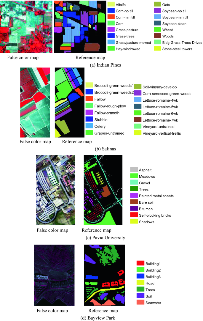

  

  Ground reference maps for the five data sets

• (b) Salinas data set: This hyperspectral image was acquired in Southern California [73]. It has a spatial size of 512 × 217 pixels with a spatial resolution of 3.7 m per pixel. Twenty water absorption bands were removed, and a 200-band image was used for the experiments. The ground reference map was composed of 54,129 pixels and 16 land-cover classes. Figure 9.14b shows a false color image and information of the labeled classes.

• (c) Pavia University Area: This HSI with 610 × 340 pixels was collected near the Engineering School, University of Pavia, Pavia, Italy. Twelve channels were removed due to noise [46]. The remaining 103 spectral channels were processed. There are 43,923 labeled samples in total, and nine classes of interest. Figure 9.14c presents false color images of this data set.

• (d) Bayview Park: The data set is from 2012 IEEE GRSS Data Fusion Contest and is one of subregions of a whole scene around downtown area of San Francisco, USA. This data set contains multispectral images with eight bands acquired by WorldView2 on October 9, 2011 and corresponding LiDAR data acquired in June 2010. It has a spatial size of 300 × 200 pixels with a spatial resolution of 1.8 m per pixel. There are 19,537 labeled pixels and 7 classes. The false color image and ground reference map are shown in Fig. 9.14d.

• (e) Recology: The source of this data set is the same as Bayview Park, which is another subregion of whole scene. It has 200 × 250 pixels with 11,811 labeled pixels and 11 classes. Figure 9.14e shows the false color image and ground reference map.

More details about these data sets are listed in Table 9.4.

Table 9.4 Information of all the data sets

9.4.2 Experimental Settings and Evaluation

To evaluate the performance of the various MKL methods for the classification task, MKL methods and typical comparison methods are shown in Table 9.5. The single kernel method represents the best performance by standard SVM, which can be used as a standard to evaluate whether a MKL method is effective or not. The number of training samples per class was varied (n = {1%, 2%, 3%} or n = {10, 20, 30}). The overall accuracy (OA [%]) and computation time were measured. Average results for a number of ten realizations are shown. To guarantee the generality, all the experiments were conducted on typical HSI data sets.

Table 9.5 Experimental methods and setting

In the first experiment of spectral classification , all spectral bands are stacked into a feature vector as input features. The feature vector was input into a Gaussian kernel with different scales. For all of the classifiers, the range of the scale of Gaussian kernel was set to [0.05, 2], and uniform sampling that selects scales from the interval with a fixed step size of 0.05 was used to select 40 scales within the given range.

In the second experiment of spatial and spectral classification , all the data sets were processed first by PCA and then by mathematical morphology (MM). The eigenvalues were arranged in descending order. The first p PCs that account for 99% of the total variation in terms of eigenvalues were reserved. Hence, the construction of the morphological profile (MP) was based on the PCs, and a stacked vector was built with the MP on each PC. Here, three kinds of SEs were used to obtain the MP features, including diamond, square, and disk SEs. For each kind of SE, a step size of an increment of 1 was used, and ten closings and ten openings were computed for each PC. Each structure of MPs with ten closings and ten openings and the original spectral features were, respectively, stacked as the input vector of each base kernel for MKL algorithms. The base kernels were 4 Gaussian kernels, i.e., the values {0.1, 1, 1.5, 2}, which corresponds to three kinds of structures of MPs and original spectral features, respectively, namely 20 base kernels for MKL methods, except for NMKL , which is with 3 Gaussian kernels, i.e., the values {1, 1.5, 2} for NMKL-Gaussian, and 4 linear base kernels function for NMKL-Linear.

Heterogeneous features were used in the third experiment, including spectral features, elevation features, normalized digital surface model (nDSM) from LiDAR data, and spatial features of MPs. MPs features are extracted from original multispectral bands and nDSM uses the diamond structure element with the sizes [3, 5, 7, 9, 11, 13, 15, 17, 19, 21]. Heterogeneous features are stacked as a single vector of features to be the input of fusion methods.

Superpixel -based spatial–spectral features were used in the fourth experiment. The Multiple SEs and multiple AFs were carried out on the extracted p PCs, respectively. Three kinds of SEs including line, square, and disk with three scales [3, 6, 9] are used. Four kinds of AFs are adopted, including (1) area of the region (related to the size of the regions), (2) diagonal of the box bounding the regions, (3) moment of inertia (as an index for measuring the elongation of the regions), (4) standard deviation (as an index for showing the homogeneity of the regions), and the setting is the same as which is presented in [59].

The summary of the experimental setup is listed in Table 9.6.

Table 9.6 Summary of the experimental setup for Sect. 9.4

9.4.3 Spectral Classification

The numerical classification results of different MKL methods for different data sets are given in Table 9.7. The performance of MKL methods is mainly determined by the ways of constructing base kernel and the solutions of weights for base kernels. The resulting base kernel matrices from the different ways of constructing base kernel contain all the information that will be used for the subsequent classification task. The weights of base kernels learned by different MKL methods represent how to combine this information with the objective of strengthening information extraction and curbing useless information for classification .

Table 9.7 OA (%) of MKL methods under multiple scale base kernel construction

Observing the results on the three data sets, some conclusions can be drawn as follows. (1) There is a situation that the classification performance of some MKL methods is not as good in terms of classification accuracies as for that of the single kernel method. This reveals that MKL methods need good learning algorithms to ensure the performance. (2) In the three benchmark HSI data sets, the best classification performance in terms of accuracies is derived from the MKL methods. This proves that using multiple kernels instead of a single one can improve performances for HSI classification and the key is to choose the suitable learning algorithm. (3) In most cases, the subspace MKL methods are superior to the comparative MKL methods and single kernel method in terms of OA.

9.4.4 Spatial–Spectral Classification

The classification results of all these compared methods on three data sets are shown in Table 9.8. And the overall time of training and test process of Pavia University data set with 1% training samples is shown in Fig. 9.15. Several conclusions can be derived. First, as the number of training samples increases, accuracy increases. Second, the MK-Boosting method has the best classification accuracy with the cost of computation time. It is also important to note that there is not a large difference between the methods in terms of classification accuracy. It can be explained that MPs can mine well, information for classification by the way of MKL and, then, the difference among MKL algorithms mainly concentrate on complexity and sparsity of the solution. The conclusion is consistent with [45]. SimpleMKL shows the worst classification performance in terms of accuracies under multiple-scale constructions in the first experiment, but is comparable to the other methods in terms of classification accuracy in this experiment. The example of SimpleMKL illustrates that a MKL method is difficult to guarantee the best classification performance in terms of accuracies in all cases. Feature extraction and classification are both important steps for classification. If the information extraction via features is successful for classification, the classifier design can be easy in terms of complexity and sparsity, and vice versa. The subspace MKL algorithms as two-stage methods have a lower complexity than one-step methods such as SimpleMKL, CS-SMKL.

Table 9.8 OA (%) of MKL methods under MPs base kernel construction

Fig. 9.15

The overall time of training and testing process in all the methods

It can be noted that the NMKL with the linear kernels demonstrates a little lower accuracy than subspace MKL algorithms with the Gaussian kernel. NMKL with the Gaussian kernels obtains comparable classification accuracy compared with NMKL with linear kernels in the Pavia University data set and the Salinas data set, but with a lower accuracy in the Indian data set. In general, using a linear combination of Gaussian kernels is more promising than a nonlinear combination of linear kernels. However, the nonlinear combinations of Gaussian kernels need to be researched further. Feature combination and the scale of the Gaussian kernels have a big influence on the accuracy of NMKL with a Gaussian kernel. And the NMKL method also demonstrates a different performance trend for different data sets. In this experiment, some tries were attempted and the results show relatively better results compared to other approaches in some situations. More work of theoretical analysis needs to be done in this area.

It can be found that among all the sparse methods, CS-SMKL demonstrated comparable classification accuracies for the Indian Pines and Salinas data sets. And for Pavia data set, as the number of training samples grows, the classification performance of CS-SMKL increased significantly and reached a comparable accuracy, too. In order to visualize the contribution of each feature type and these corresponding base kernels in these MKL methods, we plot the kernel weights of the base kernels for RMKL, DMKL, SimpleMKL, Sparse MKL, and CS-SMKL in Fig. 9.16. For simplicity, here only three one against one classifiers of Pavia University data set (Painted metal sheets vs. Bare soil, Painted metal sheets vs. Bitumen, Painted metal sheets vs. Self-blocking bricks) are listed. RMKL, DMKL, SimpleMKL and Sparse MKL used the same kernel weights as shown in Fig. 9.16a–d for all the class-pairs. From Fig. 9.16e, it is easy to find that CS-SMKL selected different sparse base kernel sets for different class-pairs, and the spectral features are important for these three class-pair. For the CS-SMKL, it only selected very few base kernels for classification purposes, while the kernel weight for the spectral features is very high. However, these corresponding kernel weights in RMKL, DMKL are much lower, and Sparse MKL did not select any kernel related to the spectral features; SimpleMKL selects the first three kernels related to the spectral features, but obviously, the corresponding kernel weights are lower than that related to the EMP feature obtained by the square SE. This is an example showing that CS-SMKL provides more flexibility in selecting kernels (features) for improving classification .

Fig. 9.16

Weights $\eta$ determined for each base kernel and the corresponding feature type. a–d A fixed set of kernel weights selected by RMKL. e The kernel weights selected for three different class-pairs by CS-SMKL

9.4.5 Classification with Heterogeneous Features

This subsection shows the performance of the fusion framework of heterogeneous features with MKL (denoted as HF-MKL) under realistic ill-posed situations, and the results compared with other MKL methods. In fusion framework of HF-MKL, RMKL was adopted to determine the weights of the base kernels on both levels of MKL in column and row. Joint classification with the spectral features, elevation features, and spatial features was carried out, and the results of classification for two data sets are shown in Table 9.9. SK represents a natural and simple strategy to fuse heterogeneous features , and it can be used as a standard to evaluate the effectiveness of different fusion strategies for heterogeneous features. With this standard, CKL is poor. The performance of CKL is affected by the weights of spectral, spatial, and elevation kernels. All the MKL methods outperform the stacked-vector approach strategy. This reveals that features from different sources obviously have different meanings and statistical significance. Therefore, they may play different roles in classification . Consequently, the stacked-vector approach is not a good choice for the joint classification . However, MKL is an effective fusion strategy for heterogeneous features , and the further HF-MKL framework is a good choice.

Table 9.9 OA (%) of different MKL methods on two data sets

9.4.6 Superpixel-Based Classification

The OA with the standard deviation for two data sets were shown in Table 9.10. The best results were given in bold. It is clear that the classification accuracy of EMP-SP-SVM is higher than EMP-SVM and the proposed framework can achieve the highest classification accuracy for both data sets, which demonstrate the effectiveness of the MMSP model. For Pavia University data set, the best results were obtained from MPSP-DMKL method, the maximum increment is 5.22% when the number of training samples was 50 per class. As the number of training samples increased, the increment decreased to 1.95%. The relative low proposed method was MPSP-CKL whose increment was between 0.92 and 2.21%. Note that in [74], for Pavia University data set, the OA of SCMK was 99.22% with 200 training samples per class. While in our proposed methods, the OA of MASP-DMKL can achieve 99.24% with only 100 training samples per class. For Salinas data set, not all the proposed methods achieved satisfactory classification results. Only these EMAP-based frameworks can outperform the other approaches. The reason might be that the geometry structure in agriculture scene is simple and mostly polygon, disk SE cannot detect the size and shape of the object exactly, but introduce wrong edges because of erosion and dilation operations, leading to imprecise spatial information. The method which showed the best classification performance is MASP-DMKL with an increment between 1.65 and 2.50%.

Table 9.10 OA (%) of two data sets

The OAs for all the data sets are presented in Table 9.11. It is clear that on both data sets, the proposed MAST-DMKL framework on four different tensor construction means outperforms the other methods, exhibiting the availability of the MAST model. In addition, the MAST-DMKL method where MASTs are filled up with original pixels can accomplish the highest classification accuracy for the other three data sets. For Indian Pines data set, when the number of training sample is 1% per class, MAST-DMKL where MAST is filled up with original pixels achieves the best classification effect with an increment of 3.34% (compared with EMAP-SVM). When the number is 2%, MAST-DMKL in which MAST is filled up with original pixels achieves the second-highest OA with an increment of 2.28% (compared with EMAP-SVM). When the number is 3%, the highest OA is obtained by MAST-DMKL of mean vectors with an increment of 2.51%. For Pavia University data set, the four kinds of MAST frameworks achieve similar classification results. With the increasing number of training samples, the increment of the OA becomes smaller, i.e., from 0.51 to 0.18% (compared with EMAP-SVM).

Table 9.11 OAS (%) of two data sets

9.5 Conclusion

In general, the MKL methods can improve the classification performance in most cases compared with single kernel method. For classification of spectral information of HSI, Subspace MKL methods using a trained, weighted combination on the average outperform the untrained, unweighted sum, namely, RBMKL (Mean MKL), and have significant superiority of accuracy and computational efficiency compared with the SimpleMKL method. Ensemble MKL method (MK-Boosting) has higher classification performance in terms of classification accuracy but an additional cost of computation time. It is also important to note that there is not a large difference in classification accuracy among different MKL methods. If we can extract effective spatial–spectral features for HSI classification , the choice of MKL algorithms mainly concentrates on complexity and sparsity of the solution. In general, using the linear combination of kernels with Gaussian kernels is effective compared to a nonlinear combination of linear kernels. However, more research needs to be carried out to fully develop the nonlinear combinations of Gaussian kernels. This is still an open problem, which is affected by many factors such as the manner in which features are combined, as well as the scale of Gaussian kernels.

Currently, with the improvement of the quality of HSI, we can extract more and more accurate features for classification task. These features could be multiscale, multi-attribute, multi-dimension and multi-components. Since MKL provides a very effective means of learning, it is natural considering to utilize these features by MKL framework. Expanding the feature spaces with a number of information diversities, these multiple features provide excellent ability to improve the classification performance. However, there exists a high redundancy of information among these multiple features, and each kind of them has different contribution to classification task. As a solution, sparse MKL methods are developed. The sparse MKL framework allows to embed a variety of characteristics in the classifier, it removes the redundancy of multiple features effectively to learn a compact set of features and selects the weights of corresponding base kernels, leading to a remarkable discriminability. The experimental results on three different hyperspectral data sets, corresponding to different contexts (urban, agricultural) and different spectral and spatial resolutions, demonstrate that the sparse methods offer good performance.

Heterogeneous features from different sources have different meanings, dimension units, and statistical significance. Therefore, they may play different roles in classification and should be treated differently. MKL performs heterogeneous features fusion in implicit high-dimensional feature representation. Utilizing different heterogeneous features to construct different base kernels can distinguish those different roles and fuse the complementary information contained in heterogeneous features . Consequently, MKL is a more reasonable choice than stacked-vector approach, and our experimental results also demonstrated this point. Furthermore, the two-stage MKL framework is a good choice in terms of OA.

References

Demir B, Erturk S (2010) Empirical mode decomposition of hyperspectral images for support vector machine classification. IEEE Trans Geosci Remote Sens 48(11):4071–4084
Hughes GF (1968) On the mean accuracy of statistical pattern recognizers. IEEE Trans Inf Theory 14(1):55–63
Kuo B, Li C, Yang J (2009) Kernel nonparametric weighted feature extraction for hyperspectral image classification. IEEE Trans Geosci Remote Sens 47(4):1139–1155
Melgani F, Bruzzone L (2004) Classification of hyperspectral remote sensing images with support vector machines. IEEE Trans Geosci Remote Sens 42(8):1778–1790
Camps-Valls G, Bruzzone L (2005) Kernel-based methods for hyperspectral image classification. IEEE Trans Geosci Remote Sens 43(6):1351–1362
Kuo B, Ho H, Li C et al (2014) A kernel-based feature selection method for SVM With RBF kernel for hyperspectral image classification. IEEE J Sel Topics Appl Earth Observ Remote Sens 7(1):317–326
Gehler PV, Schölkopf B (2009) An introduction to kernel learning algorithms. In: Camps-Valls G, Bruzzone L (eds) Kernel methods for remote sensing data analysis. Wiley, Chichester, UK, pp 25–48
Ramzi P, Samadzadegan F, Reinartz P (2014) Classification of hyperspectral data using an AdaBoostSVM technique applied on band clusters. IEEE J Sel Topics Appl Earth Observ Remote Sens 7(6):2066–2079
Xia J, Chanussot J, Du P, He X (2016) Rotation-based support vector machine ensemble in classification of hyperspectral data with limited training samples. IEEE Trans Geosci Remote Sens 54(3):1519–1531
Xue Z, Du P, Su H (2014) Harmonic analysis for hyperspectral image classification integrated with PSO optimized SVM. IEEE J Sel Topics Appl Earth Observ Remote Sens 7(6):2131–2146
Gao L, Li J, Khodadadzadeh M et al (2015) Subspace-based support vector machines for hyperspectral image classification. IEEE Geosci Remote Sens Lett 12(2):349–353
Peng J, Zhou Y, Chen CLP (2015) Region-kernel-based support vector machines for hyperspectral image classification. IEEE Trans Geosci Remote Sens 53(9):4810–4824
Guo X, Huang X, Zhang L et al (2016) Support tensor machines for classification of hyperspectral remote sensing imagery. IEEE Trans Geosci Remote Sens 54(6):3248–3264
Stork CL, Keenan MR (2010) Advantages of clustering in the phase classification of hyperspectral materials images. Microsc Microanal 16(6):810–820
Shao Z, Zhang L, Zhou X et al (2014) A novel hierarchical semisupervised SVM for classification of hyperspectral images. IEEE Geosci Remote Sens Lett 11(9):1609–1613
Yang L, Yang S, Jin P et al (2014) Semi-supervised hyperspectral image classification using spatio-spectral Laplacian support vector machine. IEEE Geosci Remote Sens Lett 11(3):651–655
Bazi Y, Melgani F (2008) Classification of hyperspectral remote sensing images using gaussian processes. IEEE Int Geosci Remote Sens Symp
Bazi Y, Melgani F (2010) Gaussian process approach to remote sensing image classification. IEEE Trans Geosci Remote Sens 48(1):186–197
Liao W, Tang J, Rosenhahn B, Yang MY (2015) Integration of Gaussian process and MRF for hyperspectral image classification. IEEE Urban Remote Sens Event
Chen Y, Nasrabadi NM, Tran TD (2011) Hyperspectral image classification using dictionary-based sparse representation. IEEE Trans Geosci Remote Sens 49(102):3973–3985
Liu J, Wu Z, Wei Z et al (2013) Spatial-spectral kernel sparse representation for hyperspectral image classification. IEEE J Sel Topics Appl Earth Observ Remote Sens 6(6):2462–2471
Chen Y, Nasrabadi NM, Tran TD (2013) Hyperspectral image classification via kernel sparse representation. IEEE Trans Geosci Remote Sens 51(11):217–231
Srinivas U, Chen Y, Monga V et al (2013) Exploiting sparsity in hyperspectral image classification via graphical models. IEEE Geosci Remote Sens Lett 10(3):505–509
Zhang H, Li J, Huang Y, Zhang L (2014) A nonlocal weighted joint sparse representation classification method for hyperspectral imagery. IEEE J Sel Topics Appl Earth Observ Remote Sens 7(6):2056–2065
Fang L, Li S, Kang X et al (2014) Spectral-spatial hyperspectral image classification via multiscale adaptive sparse representation. IEEE Trans Geosci Remote Sens 52(12):7738–7749
Li J, Zhang H, Zhang L (2015) Efficient superpixel-level multitask joint sparse representation for hyperspectral image classification. IEEE Trans Geosci Remote Sens 53(10):5338–5351
Ul Haq QS, Tao L, Sun F et al (2012) A fast and robust sparse approach for hyperspectral data classification using a few labeled samples. IEEE Trans Geosci Remote Sens 50(6):2287–2302
Yang S, Jin H, Wang M et al (2014) Data-driven compressive sampling and learning sparse coding for hyperspectral image classification. IEEE Geosci Remote Sens Lett 11(2):479–483
Qian Y, Ye M, Zhou J (2013) Hyperspectral image classification based on structured sparse logistic regression and three-dimensional wavelet texture features. IEEE Trans Geosci Remote Sens 51(42):2276–2291
Tang YY, Yuan H, Li L (2014) Manifold-based sparse representation for hyperspectral image classification. IEEE Trans Geosci Remote Sens 52(12):7606–7618
Yuan H, Tang YY, Lu Y et al (2014) Hyperspectral image classification based on regularized sparse representation. IEEE J Sel Topics Appl Earth Observ Remote Sens 7(6):2174–2182
Li J, Zhang H, Zhang L (2014) Column-generation kernel nonlocal joint collaborative representation for hyperspectral image classification. ISPRS J Int Soc Photo Remote Sens 94:25–36
Li J, Zhang H, Huang Y, Zhang L (2014) Hyperspectral image classification by non-local joint collaborative representation with a locally adaptive dictionary. IEEE Trans Geosci Remote Sens 52(6):3707–3719
Li J, Zhang H, Zhang L et al (2014) Joint collaborative representation with multitask learning for hyperspectral image classification. IEEE Trans Geosci Remote Sens 52(9):5923–5936
Li W, Du Q (2014) Joint within-class collaborative representation for hyperspectral image classification. IEEE J Sel Topics Appl Earth Observ Remote Sens 7(6):2200–2208
Li W, Du Q, Xiong M (2015) Kernel collaborative representation with Tikhonov regularization for hyperspectral image classification. IEEE Geosci Remote Sens Lett 12(1):48–52
Liu J, Wu Z, Li J, Plaza A, Yuan Y (2016) Probabilistic-kernel collaborative representation for spatial-spectral hyperspectral image classification. IEEE Trans Geosci Remote Sens 54(4):2371–2384
He Z, Wang Q, Shen Y, Sun M (2014) Kernel sparse multitask learning for hyper-spectral image classification with empirical mode decomposition and morphological wave-let-based features. IEEE Trans Geosci Remote Sens 52(8):5150–5163
Xiong M, Ran Q, Li W et al (2015) Hyperspectral image classification using weighted joint collaborative representation. IEEE Geosci Remote Sens Lett 12(6):1209–1213
Wright J, Ma Y, Mairal J et al (2010) Sparse representation for computer vision and pattern recognition. Proc IEEE 98(6):1031–1044
Wright J, Yang AY, Ganesh A et al (2009) Robust face recognition via sparse representation. IEEE Trans Pattern Anal Mach Intell 31(2):210–227
Zhang L, Yang M, Feng X, Ma Y, Zhang D (2012) Collaborative representation based classification for face recognition. Comput Sci
Baron D, Duarte MF, Wakin MB, Sarvotham S, Baraniuk RG (2009) Distributed compressive sensing. arXiv:0901.3403 [cs.IT]
Gu Y, Wang Q, Xie B (2017) Multiple kernel sparse representation for airborne Li-DAR data classification. IEEE Trans Geosci Remote Sens 5(2):1085–1105
Gonen M, Alpaydin E (2011) Multiple kernel learning algorithms. J Mach Learn Res 12:2211–2268
Camps-Valls G, Gomez-Chova L, Munoz-Mari J et al (2006) Composite Kernels for hyperspectral image classification. IEEE Geosci Remote Sens Lett 3(1):93–97
Wang J, Jiao L, Wang S et al (2016) Adaptive nonlocal spatial–spectral kernel for hyperspectral imagery classification. IEEE J Sel Topics Appl Earth Observ Remote Sens 9(9):4086–4101
Camps-Valls G, Gomez-Chova L, Munoz-Mari J et al (2008) Kernel-based framework for multitemporal and multisource remote sensing data classification and change detection. IEEE Trans Geosci Remote Sens 46(6):1822–1835
Fang L, Li S, Duan W et al (2015) Classification of hyperspectral images by exploiting spectral-spatial information of superpixel via multiple kernels. IEEE Trans Geosci Remote Sens 53(12):6663–6674
Valero S, Salembier P, Chanussot J (2013) Hyperspectral image representation and processing with binary partition trees. IEEE Trans Image Process 22(4):1430–1443
Zhou Y, Peng J, Chen CLP (2015) Extreme learning machine with composite kernels for hyperspectral image classification. IEEE J Sel Topics Appl Earth Observ Remote Sens 8(6):2351–2360
Li H, Ye Z, Xiao G (2015) Hyperspectral image classification using spectral-spatial composite kernels discriminant analysis. IEEE J Sel Topics Appl Earth Observ Remote Sens 8(6):2341–2350
Zhang Y, Prasad S (2015) Locality preserving composite kernel feature extraction for multi-source geospatial image analysis. IEEE J Sel Topics Appl Earth Observ Remote Sens 8(3):1385–1392
Gu Y, Wang C, You D et al (2012) Representative multiple kernel learning for classification in hyperspectral imagery. IEEE Trans Geosci Remote Sens 50(72):2852–2865
Gu Y, Wang Q, Wang H et al (2015) Multiple kernel learning via low-rank nonnegative matrix factorization for classification of hyperspectral imagery. IEEE J Sel Topics Appl Earth Observ Remote Sens 8(6):2739–2751
Gu Y, Wang Q, Jia X et al (2015) A novel MKL model of integrating LiDAR data and MSI for urban area classification. IEEE Trans Geosci Remote Sens 53(10):5312–5326
Wang Q, Gu Y, Tuia D (2016) Discriminative multiple kernel learning for hyperspectral image classification. IEEE Trans Geosci Remote Sens 54(7):3912–3927
Rakotomamonjy A, Bach FR, Canu SE et al (2008) SimpleMKL. J Mach Learn Res 9(11):2491–2521
Liu T, Gu Y, Jia X et al (2016) Class-specific sparse multiple kernel learning for spectral-spatial hyperspectral image classification. IEEE Trans Geosci Remote Sens 54(12):7351–7365
Wang L, Hao S, Wang Q, Atkinson PM (2015) A multiple-mapping kernel for hyper-spectral image classification. IEEE Geosci Remote Sens Letters 12(5):978–982
Gu Y, Liu T, Jia X, Benediktsson JA, Chanussot J (2016) Nonlinear multiple kernel learning with multiple-structure-element extended morphological profiles for hyperspectral image classification. IEEE Trans Geosci Remote Sens 54(6):3235–3247
Do TTH (2012) A unified framework for support vector machines, multiple kernel learning and metric learning. In: A unified framework for support vector machines, multiple kernel learning and metric learning, vol. Docteur, Series A unified framework for support vector machines, multiple kernel learning and metric learning. Universite De Geneve
Cristianini N, Shawe-Taylor J (1999) An introduction to support vector machines and other kernel-based learning methods. Cambridge University Press, New York, NY, USA
Gu Y, Gao G, Zuo D, You D (2014) Model selection and classification with multiple kernel learning for hyperspectral images via sparsity. IEEE J Sel Topics Appl Earth Observ Remote Sens 7(6):2119–2130
Gu Y, Liu H (2016) Sample-screening MKL method via boosting strategy for hyperspectral image classification. Neurocomputing 173:1630–1639
Zhang Y, Yang HL, Prasad S et al (2015) Ensemble multiple kernel active learning for classification of multisource remote sensing data. IEEE J Sel Topics Appl Earth Observ Remote Sens 8(2):845–858
Cortes C, Mohri M, Rostamizadeh A (2009) Learning non-linear combinations of kernels. In: Proceedings of advances in neural information processing systems, pp 396–404
Xu Z, Jin R, Yang H et al (2010) Simple and efficient multiple kernel learning by group Lasso. In: Proceedings of the 27th international conference on machine learning
Schapire RE (1990) The strength of weak learnability. Mach Learn 5(2):197–227
Freund Y, Schapire RE (1997) A decision-theoretic generalization of on-line learning and an application to boosting. J Comput System Sci 55(1):119–139
Li J, Huang X, Gamba P et al (2015) Multiple feature learning for hyperspectral image classification. IEEE Trans Geosci Remote Sens 53(3):1592–1606
Xia H, Hoi SCH (2013) MKBoost: a framework of multiple kernel boosting. IEEE Trans Knowl Data Eng 25(7):1574–1586
Gamba P (2004) A collection of data for urban area characterization. IEEE Int Geosci Remote Sens Symp (IGARSS), pp 69–72
Liu T, Gu Y, Chanussot J et al (2017) Multimorphological superpixel model for hyperspectral image classification. IEEE Trans Geosci Remote Sens 55(12):6950–6963
Jia S, Zhu Z, Shen L, Li Q (2014) A two-stage feature selection framework for hyperspectral image classification using few labeled samples. IEEE J Sel Topics Appl Earth Observ Remote Sens 7(4):1023–1035
Cristianini N, Shawe-Taylor J, Elisseeff A, Kandola J (2002) On kernel-target alignment. In: Dietterich TG, Becker S, Ghahramani Z (eds) Advance in neural information processing systems, vol 14, pp 367–373
Li W, Du Q (2016) A survey on representation-based classification and detection in hyperspectral remote sensing imagery. Pattern Recogn Lett 83:115–123
Author information
Authors and Affiliations
Corresponding author
Editor information
Editors and Affiliations
Rights and permissions
Copyright information
© 2020 Springer Nature Switzerland AG
About this chapter
Cite this chapter
Liu, T., Gu, Y. (2020). Multiple Kernel Learning for Hyperspectral Image Classification. In: Prasad, S., Chanussot, J. (eds) Hyperspectral Image Analysis. Advances in Computer Vision and Pattern Recognition. Springer, Cham. https://doi.org/10.1007/978-3-030-38617-7_9
Download citation
DOI: https://doi.org/10.1007/978-3-030-38617-7_9
Published:
Publisher Name: Springer, Cham
Print ISBN: 978-3-030-38616-0
Online ISBN: 978-3-030-38617-7
eBook Packages: Computer ScienceComputer Science (R0)