
Abstract
This chapter discusses aspects of sustainability and “green” that are relevant to and arise within location problems. More specifically, it describes ways in which some environmental criteria, in particular emissions, can be quantified and integrated with location models. The chapter also presents design problems in which location decisions arise as one of the key ingredients in improving the environmental performance of distribution systems.
Access provided by Autonomous University of Puebla. Download chapter PDF
Keywords
1 Sustainability and “Green” in Location Problems
Facility location problems arise in the broader context of logistics network design, where the primary aim is to move freight from points of origin to points of destination. The activities relevant to production, transportation and distribution of the goods over a logistics network inevitably results in undesirable effects on the environment, generally referred to as externalities, which include the following:
Logistics operations deplete natural resources that are needed for the underlying infrastructure and the various activities run on the network. The former includes construction of facilities such as hubs, depots or ports, as well as highways and railway tracks, relying on the extraction and the use of various materials needed for the construction, use of land on which they are built, and potential change or damage to the ecosystem around them. The activities themselves require energy for the movement of goods, primarily fuel.
Most logistics activities induce some form of noise that is detrimental to human health and well-being. In addition, the vibration caused by the movement of goods, e.g., freight trains passing through cities, lorries operating in urban areas, may damage the buildings around them in the long run.
Pollution is perhaps the most prominent of all externalities, not least for their direct and indirect impacts on the environment, but also the role they are deemed to play in climate change. Air pollution is caused by various types of gases, including greenhouse gases such as methane, ozone, carbon dioxide and nitrous oxide, others such as carbon monoxide, nitrogen oxide and sulphur oxide, and particulate matter, emitted by production and transportation activities. They are responsible for environmental impacts such as the greenhouse gas effect, acidification, summer smog and other toxic effects.
Accidents occur predominantly within transportation, but also manufacturing and production environments, and are responsible for injury and death for all forms of life. Their severity could be far more significant in the context of obnoxious facilities and hazardous materials, with potentially disastrous consequences.
There are various ways to mitigate or lessen the externalities above within the broader context of logistics management, including technological solutions and management strategies, which is beyond the remit of this chapter. The interested reader is referred to McKinnon et al. (2015) and Psaraftis (2016) for a broader and a more in-depth treatment of the topic.
To achieve greener ways of operation in the particular context of facility location, it is pertinent at this point to differentiate between the two types of research directions listed below:
Reducing externalities from a logistics network by locating facilities, caused by the amount of inbound and outbound of goods and the way in which they are moved within the network.
Reducing externalities from located facilities that appear within a logistics networks, mainly from energy consumption (lighting, heating, cooling, use of equipment for production and handling of goods), water consumption, and use of land.
The rest of this chapter will focus on the first research direction above, namely those that concern decisions around facility location and the impact thereof on the environmental performance of the logistics networks within which the facilities are to be installed and used. The second research direction will not be covered within this chapter for two reasons. First, some of the decisions to reduce the externalities from facilities requires adopting new technologies, including improving energy efficiency (e.g., use of eco-friendly lighting), switching to energy-efficient mechanical equipment, harnessing green energy sources and incorporating sustainability considerations into building design (Baker and Marchant 2015). Second, even if non-technological solutions were to be adopted, the issues relate to the interior design, as opposed to the location of a facility, and involve decisions ranging from the type and shape of the construction, to optimizing layouts within facilities.
It is important at this point to stress on the fact that this chapter does not concern itself directly with the broader issues around sustainability apart from those that are indirectly linked with the green agenda. From an environmental perspective, our understanding of the former term following Jaehn (2016) revolves around the ability of the environment around a logistics system that allows the system to maintain its operations ad infinitum, or, in practical terms, for very long periods of time. It is obvious that, in the long run, the scarcity of the resources involved in running a logistics system makes it unsustainable ipso facto, in the strict sense of the word. Improving sustainability of a system may be achieved through novel solutions, including the use of unconventional technologies (such as use of alternative fuels or harnessing and using new sources of energy), and we will indeed touch on these aspects later in the chapter when discussing location problems in the context of alternative fuel vehicles. In contrast, greening of a given system, at least in the way that we interpret and treat in this chapter, will be to lessen or mitigate the environmental externalities of that system through better planning, and one that does not necessarily involve a fundamental change in the way that the operations are set up and run. One example in the context of facility location may simply be to change the number and location of facilities to improve the environmental performance of a distribution system.
2 Environmental Considerations in Location Problems
An explicit consideration of externalities within location problems is possible to the extent that their impacts are quantifiable, and that it is possible to estimate the quantity of the amount through analytical models as a function of decisions made within location problems. If such analytical models exist, then they can generally be integrated within existing models of various facility location problems. In the rest of this section, we will focus on emissions as the main environmental impact, not least given their prominence within environmental externalities, but also the relative easiness with which they can be quantified.
Emissions are, in most cases, proportional to the amount of energy consumed by a given logistics operation. In conventional road transport, for example, the amount of pollutants emitted is dependent on the amount of fuel consumed. This makes it easier to estimate the amount of emissions from a given operation, if the level of activity is known and there exist emission factors. This is the main principle behind what is known as emission factor models, for which there exist two types of models:
The first type is used when the actual amount of energy or fuel α is known (e.g., in kWh or litres), which is then multiplied by the emission factor ϕ (e.g., in grams per kWh), yielding the total emissions E = α × ϕ for a given activity. This actual energy consumed can be calculated using historical data, such as readings from storage tanks for lorries or electricity bills for facilities, and is therefore calculated retrospectively.
If the actual amount of energy consumed cannot be calculated, or is not available, then one can resort to the second type of emissions model that uses average conversion factors that are pre-defined depending on the type of activity. The UK Government’s Department for Business, Energy & Industrial Strategy defines the emission factors separately for fuel, electricity, heat, steam, passenger transport, freight land transport, sea transport and air transport, and for various types of gases such as carbon dioxide (CO2), methane (CH4) and nitrogen oxide (N2O), and for different types of vehicles and for various load levels. For road transport, the emission factors are defined for one kg of CO2 per vehicle kilometers traveled, or one kg of CO2 per tonne.kilometer. For air freight, rail transport or sea transport, the emissions factors are defined for one kg of CO2, CH4 or N2O per tonne.kilometer. The reader is referred to Hill et al. (2017) for further details.Footnote 1 For illustrative purposes, Fig. 20.1 shows the resulting amount of CO2 emissions for two different types of vehicles under different load levels estimated by using the factors given by Hill et al. (2017) traveling from 10 to 100 km.
Fig. 20.1 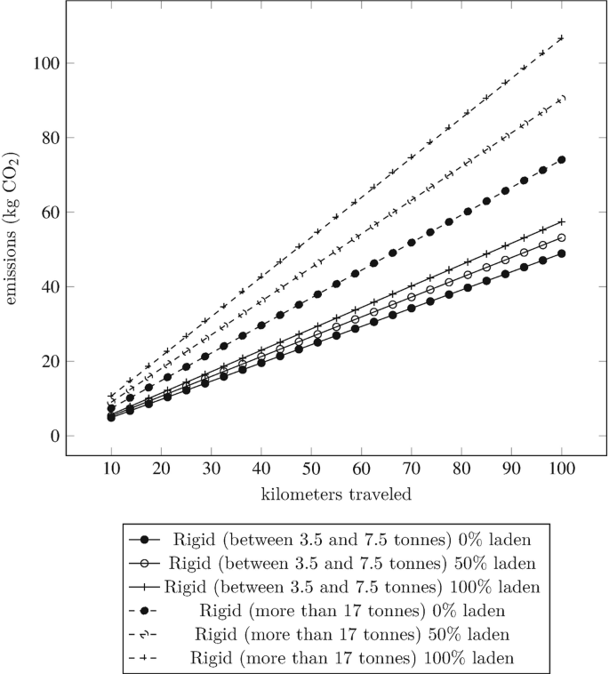
CO2 emissions for various goods vehicles estimated using the factor model

There exist other types of analytical models to estimate emissions that are more detailed as compared to emission factor models. One such type that is used within road transportation is the macroscopic or average speed models, a class of models that are primarily regression based, and use average speed v of a vehicle as a primary determinant to estimate emissions. One such model appears in an emissions inventory guidebook by the European Environment Agency (Ntziachristos et al. 2017), where hot emissions E(v) (g/km) are calculated on the basis of average speed v (km/h) using the following generic expression,
where a1–a7 are coefficients that differ by fuel, vehicle class and engine technology,Footnote 2 and β is a correction factor applied, if necessary, to account for different types of road (i.e., urban, rural and highway). Figures 20.2 and 20.3 show the resulting CO emissions output by the average speed model (20.1) for different types of goods vehicles.

Emissions calculated using the average speed model for vehicles with conventional and older engine technology

Emissions calculated using the average speed model for vehicles with newer engine technology
At a micro-level, a more detailed class of models is available that generally named as microscopic or instantaneous emissions models. These models are derived from mechanical physics of automobile engines, and take a significant number and range of parameters into account, such as vehicle characteristics (mass, drag force, rolling resistance, engine efficiency) as well as external factors (air density, gravitational constant), in order to estimate emissions, often on a second-by-second basis. Further details on microscopic models can be found in Demir et al. (2014). However, as facility location problems typically involve strategic (and sometimes tactical) decisions made to last over relatively long time-spans, micro-level models may be too detailed a representation of vehicle dynamics to influence such long-term decisions and may not necessarily be the most suitable types of models to use. There may, however, be exceptions to this situation if location problems arise at an operational level of decision making, in which case an integration of facility location and micro-level emission models may be appropriate.
2.1 Accounting for Emissions in Facility Location Problems
Location problems almost always involve decisions pertaining to installation of facilities that are typically modeled by a vector y of binary variables, which induces a fixed cost f(y) that generally, but not always, linearly increases with the number and type of facilities. The second set of decisions relate to the assignment of customers to installed facilities, represented by the vector x, which induces an operational cost c(x) that may include, amongst others, shipment costs, including drivers, fuel and vehicle acquisition. The assignment decisions x also dictate the volume of products that flow between a facility and a customer, which affects both fuel consumption and emissions, either through choice of vehicle or load, or both. If g(x) denotes the amount of emissions arising from the shipment of products, then a simplified representation of a facility location model that captures the trade-off between operational costs and emissions can be presented as follows:

where A, B and D are matrices of suitable proportions. The model above is a bi-objective formulation, with the first objective ψ1 reflecting the operational costs and the second objective ψ2 denoting the emissions. The first set of constraints are relevant to the assignment of customers to facilities and the second set of constraints ensure that each customer is assigned to a facility that is installed. If there is a suitable weighting γ of emissions (e.g., cost) to make it commensurate with c(x), then the two objectives can be re-written as follows,

particularly as, in most cases, the amount of emissions from a vehicle is proportional to fuel consumption. One extreme solution to the model above is to reduce the number of facilities to the minimum possible (e.g., only one if there are no capacity restrictions), which will achieve objective \(\psi ^{\prime }_1\) but significantly increase the transportation costs c(x) and emissions g(x). In the other extreme, increasing the number of facilities (e.g., one at the site of each customer) will maximize the facility costs f(y) but simply drive \(\psi ^{\prime }_2\) equal to 0. The two extremes show that the problem is truly bi-objective, i.e., the two objectives \(\psi ^{\prime }_1\) and \(\psi ^{\prime }_2\) are contradictory, and the solution highly depends on the relative importance of the operational costs and the weight of the environmental factors.
The approach adopted by Tricoire and Parragh (2017) is along the lines of the general model introduced above in formulating a bi-objective hub location routing problem, where one objective is related to minimization of operational costs that include that of establishing hubs and space acquisition costs, and the other minimizes CO2 emissions induced by the empty and loaded running of the vehicles. This study treats the emissions as being fixed per unit of distance and per unit load of weight, and derives insights on the trade-offs between the number of hubs used and the resulting emissions, with an overall conclusion that “investing in facilities does reduce future pollution”.
The studies by Koç et al. (2014) and Toro et al. (2017) investigate similar problems in that they integrate facility location decisions with those of fleet size and mix and routing (in the former) and vehicle routing (in the latter). In contrast to the work of Tricoire and Parragh (2017), however, they both use a more detailed representation of fuel consumption and emissions that is minimized as part of the overall problem. In Koç et al. (2014), this entails the use of a comprehensive modal emissions model as part of the (single) objective for estimating fuel consumption from heavy-good vehicles operating in urban areas, part of which requires to optimize speeds of the vehicles. The authors conclude by stating that it is preferable to locate depots outside the city centre and to use heterogeneous fleets over homogeneous fleets. This study shows the impact choice of the location of the facilities can have on the overall choice of a distribution strategy within urban areas. In Toro et al. (2017), vehicle speed is not part of the decision problem whereby the vehicles are assumed to travel at constant speed, and that fuel consumption is estimated on the basis of the distance traversed and the load carried by a vehicle. The latter work treats the problem as being bi-objective, with one objective minimizing operational costs, and the other minimizing fuel and emissions. One interesting finding of Toro et al. (2017) is that increasing the number of vehicles used results in improved fuel economy and hence less emissions, mainly due to the shorter trips that the vehicles will have to perform.
Studies that look at the integration of facility location problems with consideration of externalities are few and far between, some of which are described above, but more research is required in this area, not only for development of methodological approaches to solve such problems but perhaps more importantly, understanding the trade-offs involved in making strategic and operational decisions to improve economical and environmental performance of distribution systems.
3 Reverse Logistics Network Design
Reverse logistics refers to all operations involved in the return of products and materials from a point of use to a point of recovery or proper disposal. The purpose of recovery is to recapture value through options such as reusing, repairing, refurbishing, re-manufacturing, and recycling. Reverse logistics includes the management of the return of end-of-use or end-of-life products as well as defective and damaged items, or packaging materials, containers, and pallets.
Reverse logistics activities aim to lessen or mitigate the environmental externalities as such operation of reverse logistics networks lead to reduced use of natural resources as well as pollution prevention through the reduction of waste. Major driving forces behind reverse logistics include not only environmental consciousness but also economic factors and government legislations. As stated by De Brito and Dekker (2004), companies become active in reverse logistics because they can make a profit and/or because they are forced to focus on such functions, and/or because they feel socially motivated. These factors are usually intertwined. For example, a company can be compelled to reuse a certain percentage of components in order to achieve a recovery target set by the legislation. This will lead to a decrease in the cost of purchasing components and in waste generation. Jayaraman and Luo (2007) suggest that proper management of reverse logistics operations can lead to greater profitability and customer satisfaction, and at the same time be beneficial to the environment.
In a reverse logistics network, end-of-life or end-of-use products can be generated at private households and at commercial, industrial, and institutional sources, which are referred to as generation points. Products are usually collected at special storage facilities called collection or inspection centers. Products are then sent for proper recovery through reusing, repairing, refurbishing, remanufacturing, or recycling. Inspected or recovered products and components can then be sold to suppliers, to (re)manufacturing facilities, or to customers in the secondary market. A generic reverse logistics network is depicted in Fig. 20.4.

A generic reverse logistics network
The design of a reverse logistics network is a complex problem comprising the determination of the optimal locations of different types of facilities as well as the integration between these facilities. The facilities to be located include but not limited to collection, inspection, recovery, (re)manufacturing, recycling, and disposal centers. The decisions to be made include determining the number, size, and capacities of the facilities to be located, the amount of products to be recovered at each facility, and the amount of products and/or components to be sent in-between these facilities.
In the next sub-section, we present a generic reverse logistics network design model and in the following section we discuss its possible extensions.
3.1 A Generic Reverse Logistics Network Design Model
Multiple commodities need to be considered in the configuration of a reverse logistics network. These commodities include used, inspected, repaired, or refurbished products, components, or raw materials and are represented by the set P. In order to represent a different state (inspected, repaired, refurbished, etc.) of a certain item, a different product type needs to be defined within this set.
Let R represent the set of available recovery options. This may include conventional options, such as repair, refurbish, and recycle as well as other options such as inspection, disassembly, selling to suppliers, to the secondary market or to external (re)manufacturing facilities, and disposal. Even though the latter options may not be regarded as recovery alternatives, in order to provide a generic model incorporating all the decisions plausible in real-life reverse logistics networks, we include these in the set R.
Other sets of parameters include Nr the set of potential locations for recovery option r ∈ R; Er the set of existing facilities with recovery option r ∈ R; Ir the set of selectable facilities with recovery option r ∈ R, Ir = Nr ∪ Er; Jr the set of non-selectable locations with recovery option r ∈ R (e.g. secondary market, disposal); and L the set of all locations, \(L = \cup _{r \in R} \, \left ( I_r \, \cup \, J_r \right )\). Some recovery options may be operated by third-party logistics providers. Such external facilities belong to the set Jr. Moreover, it is assumed that generation points are also included in this set of non-selectable facilities.
The parameters required for the mathematical model are as follows:
g ℓp | Amount of product p ∈ P generated at location ℓ ∈ L |
β rqp | Number of units of product p ∈ P obtained by processing one unit of product q ∈ P using recovery option r ∈ R |
K rℓ | Capacity of recovery option r ∈ R at location ℓ ∈ L |
T rp | Recovery target for product p ∈ P with recovery option r ∈ R |
H rℓp | Revenue from recovering one unit of product p ∈ P with recovery option r ∈ R at location ℓ ∈ L (e.g., revenue from recycling or from the secondary market) |
S rℓp | Cost of recovering one unit of product p ∈ P with recovery option r ∈ R at location ℓ ∈ L |
F ri | Fixed setup cost of establishing recovery option r ∈ R in location i ∈ Nr |
\(C_{\ell \ell ^{\prime } p}\) | Unit cost of transporting product p ∈ P from location ℓ ∈ L to location ℓ′∈ L |
Transitions between the stages of products and reverse bills-of-materials (BOMs) are taken into account by the parameter β. For example, a damaged product can be converted into a repaired product through the recovery option repair, or a used product can be disassembled into its components at a disassembly facility. There are recovery targets, usually set by the legislations, for each type of product and recovery option. Revenues may be obtained through some recovery options, e.g., by selling products or components to recycling facilities, to the secondary market or to external (re)manufacturing facilities. Some recovery options may also incur costs as in the case of product disposal.
The decision variables of the model are:
The reverse logistics network design problem can be formulated as a mixed-integer linear program as follows:
The objective function (20.2) maximizes the total profit. It sums the revenues obtained from various recovery options (e.g., by sending products to recycling facilities, by selling products to the secondary market) and subtracts the total cost of establishing and operating the reverse logistics network. The latter comprises the cost of recovery (e.g. disposal), setting up new recovery options at facilities, and transporting products.
Equalities (20.3) are the flow balance constraints. For each location and product, the total inflow comprises the amount of product generated at that location, the total amount of product obtained after processing various items, and the total amount of product shipped to this location from other locations. The total inflow is equal to the total outflow, which includes the total amount of product recovered at that location and the total amount of product shipped to other locations. Constraints (20.4) ensure that the recovery target for each product category and recovery option is met. Recovery targets are usually stipulated by legislations for different types of recovery options. Inequalities (20.5) and (20.6) are the capacity constraints for new and existing recovery options, respectively. Constraints (20.7)–(20.8) impose that products can only be shipped from operated facilities. Lastly, conditions (20.9)–(20.11) set the domains of the decision variables.
The proposed model is generic in the sense that it includes multiple types of products and components at different stages (inspected, repaired, refurbished, etc.). Moreover, it considers reverse BOMs and transitions between the stages of products through various recovery options. The problem is modeled with a profit oriented objective function accounting for the revenues from different recovery options in addition to costs.
In terms of problem complexity, the above model is NP-hard, being a generalization of the simple plant location problem (see Chap. 3). General purpose optimization software (e.g., CPLEX or Gurobi) can however be used to solve small to medium-sized instances of this model within reasonable times. For large-sized instances there may be a need for customized algorithms and heuristics. The following section discusses some extensions of the above model.
3.2 Extensions
The reverse logistics network design model introduced in the previous section can be extended in manifold ways. Analogous with the traditional facility location models, the above formulation can be generalized to include capacity selection and extension decisions, a multi-period/dynamic setting, uncertainty associated with the problem parameters, multiple objectives, etc. These extensions are already well-discussed within the other chapters of this book. We briefly discuss some of such extensions within the context of reverse logistics network design below to provide some exemplary references.
The design of a reverse logistics network can be embedded in a multi-period planning horizon. Such a setting is meaningful since the establishment of new facilities is typically a long-term project involving time-consuming activities and requiring the commitment of substantial capital resources. In this case, strategic decisions can be constrained by the budget available in each time period. A multi-period setting is also appropriate for planning the re-design of a reverse logistics network that is already in place. In this context, existing facilities may have their capacities expanded, reduced or even moved to new sites over several time periods. In turn, new facilities can be established through successive sizing. Multi-period models in reverse logistics network design were proposed, for example, by Lee and Dong (2009), Salema et al. (2010), and Alumur et al. (2012).
A distinguishing feature of reverse logistics network design problems is that there are various sources of uncertainty for the supply arising at the upper echelon facilities (e.g., uncertainty in the amount and in the quality of returned products). Studies addressing uncertainty issues in the context of reverse logistics network design include Realff et al. (2004), Listeş and Dekker (2005), Listeş (2007), Salema et al. (2007), El-Sayed et al. (2010), and Fonseca et al. (2010).
Many actors are involved in the design and operation of a reverse logistics network. Even though extended producer responsibilities defined in the legislations of various countries give the responsibility of recovering used products to original equipment manufacturers, governments need to establish the necessary infra-structure. Responsibilities can be shared among different parties, such as producers, distributors, third-party logistics providers, or municipalities, in designing and operating the reverse logistics networks. Multiple actors lead to decision problems with multiple objectives. Although there are some studies that consider the multi-objective nature of this design problem (e.g., Pati et al. 2008, Fonseca et al. 2010, Tari and Alumur 2014), this issue can certainly require further attention.
A major extension of reverse logistics network design is to integrate reverse flows with forward flows of the supply chain. The term closed-loop supply chain refers to a network comprising both forward and reverse flows. Figure 20.5 depicts the structure of such a network. The cost of processing a return flow in a supply chain designed by considering only forward flows can be much higher than processing a flow in the forward direction. Thus, supply chain networks that include flows in the reverse direction should ideally be designed by integrating forward and reverse logistics activities. The generic model introduced above for the reverse logistics network design problem can certainly be extended to the design of closed-loop supply chains. The interested reader is referred to Krikke et al. (2003), Easwaran and Üster (2009), and Salema et al. (2010) presenting models determining the locations of facilities within closed-loop supply chain networks.

A closed-loop supply chain network
For other extensions and special cases on reverse logistics network design, the interested reader is referred to the reviews by Fleischmann et al. (2004), Bostel et al. (2005), Akçalı et al. (2009), and Aras et al. (2010).
4 Location Problems Related to Alternative Fuel Vehicles
One recent class of problems within which location arise as part of the planning decisions is relevant to alternative fuel vehicles (AFVs), which either run on fuel as opposed to traditional petroleum-based fuels (petrol or Diesel fuel) or alternative technologies to power an engine that does not involve solely petroleum (Wikipedia 2017). The types of AFVs include those running on biofuel, natural gas, hydrogen (fuel cell electric), hybrid electric, plug-in hybrid electric (PHE), and battery electric (BE), also known as Zero Emission Vehicles (ZEVs) (Hackbarth and Madlener 2013; Guerra at al. 2016). AFVs are readily used in various applications including goods distribution and public transportation as well as personal transport (e.g., Pelletier et al. 2016, Tzeng et al. 2005). This section briefly discusses location problems that arise within the context of AFVs.
Similar to the conventional vehicles that are powered by petroleum fuels, refueling is also important for AFVs, if not more critical, to ensure continuity of operation without disruption. Location analysis therefore plays a significant role for installing refueling or recharging stations, in particular for PHEVs and BEVs where the refueling (charging) times can be significant. Basic location models like the p-median problem (see Chap. 2) can certainly be employed for determining the optimal locations of refueling stations (e.g., Goodchild and Noronha 1987, Nicholas et al. 2004). The motivation behind using the p-median model is the assumption that the consumers generally prefer to refuel near their homes (Upchurch and Kuby 2010).
In traditional location problems, demand is generated at nodes of the network. In contrast, the demand arising from the need to refuel AFVs does not originate from the fixed nodes but from traffic flows. Hodgson (1990) describes a so-called flow capturing location model (FCLM) to model the flow-based demand, where the aim is to locate p facilities to maximize the total demand captured (covered), and where a unit of demand to be covered is defined as the fixed path from a given origin to a destination. It is assumed that a facility placed at a node in the network covers all the flow which passes through that node; it suffices therefore to locate one facility on a path. Location problems that assume flow-based demand have later been named as flow interception problems (see, e.g., Berman et al. 1995). Kuby and Lim (2005) introduced the flow refueling location model (FRLM) by extending the FCLM to the context of generic range-limited AFVs. The FRLM defined by Kuby and Lim (2005) optimally locates p refueling stations on a network so as to maximize the total flow volume refueled for predetermined origin-destination paths. The FRLM recognizes the fact that it may be necessary to stop at more than one facility for refueling and, thus, unlike the FCLM, it allows for locating more than one facility on a path. Kuby and Lim (2005) also describe a mixed-integer programming model for the problem which assumes that all feasible facility combinations that can be used to refuel vehicles on each given origin-destination path are exogenously determined. Since generation of all these feasible combinations requires significant computational memory and time, different solution methods are proposed in the literature to overcome the difficulty (see Capar and Kuby 2012; Capar et al. 2013; Kim and Kuby 2012; Lim and Kuby 2010; MirHassani and Ebrazi 2012). In particular, Capar et al. (2013) and MirHassani and Ebrazi (2012) provide alternative formulations for the FRLM both of which drastically increase the computational efficiency.
Variations of the FRLM include those that allow locating refueling stations along arcs as well as on nodes of the network (Kuby and Lim 2007), imposing capacity constraints that limit the number of vehicles refueled at each station (Upchurch et al. 2009), incorporating locomotive refueling scheduling decisions in railroad networks (Nourbakhsh and Ouyand 2010), allowing deviation from the shortest path up to a tolerance that the drivers are willing to accept (Yıldız et al. 2016), generalizing it to account for plug-in hybrid electric vehicles (Arslan and Karaşan 2016), and assuming a probabilistic travel range for the vehicle (Lee and Han 2017).
The FRLM is a maximal covering type model (see Chap. 5 for more information on the covering location problems). An alternative way to approach the AFV refueling station location problem is through a flow-based set covering model, as was done by Wang and Lin (2009). The objective of this problem is to minimize the total cost of locating refueling stations where all flow-refueling demand is to be covered by the stations within a specific coverage distance for fixed origin-destination paths. Other studies using a flow-based set covering model for the location of refueling stations include Wang and Wang (2010), Wang and Lin (2013), MirHassani and Ebrazi (2012) and Li and Huang (2014).
The refueling station location problem can also be formulated within location-routing type models, referred as location-routing problem with intermediary facilities (see Chap. 15), more specifically, by extending such models to include additional considerations specific to AFVs (see, e.g., Kand and Recker 2014; Schiffer and Walther 2017).
In addition to determining the locations of refueling stations, one other relevant problem arising within the context of AFVs is to determine the locations of battery swapping or switching stations, where depleted batteries can be exchanged for recharged ones during a journey. Mak et al. (2013) introduced this problem and developed robust optimization models that aid the planning process for deploying battery-swapping infrastructure. Variants of this problem can be found in Yang and Sun (2015) and Hof et al. (2017).
The particular characteristics of AFVs can be incorporated within any of the location models as additional constraints, for example, considering multiple types of charging facilities with varying charging rates (Liu and Wang 2017), partial or full charging options (Keskin and Çatay 2016; Schiffer and Walther 2017), battery life-span or battery degradation concepts (Kong et al. 2017).
Finally, and although not necessarily a location problem in the traditional sense, it is worth mentioning a study by Chen et al. (2016) that introduces a network design problem related to AFVs, which consists of determining an optimal deployment of charging lanes for electric vehicles in transportation networks. This follows a recent development in the ‘charging-while-driving’ technology, which envisages deploying charging lanes in regional or even urban road networks of the future which electric vehicles can use. In this case, the lanes themselves may be seen as facilities. It is clear that technologies that are fast developing for AFVs will give rise to other such interesting problems in the near future.
5 Research Prospects
Environmental issues arising within location problems are broad and complex, but need to be captured and addressed nevertheless. Green location problems necessitates an explicit consideration of micro-level and firm-based environmental performance measures, such as internal consumption of resources including energy, water, land and building materials, as well as the wider macro-level impacts that extend beyond a facility, such as “land use, atmospheric emissions, waste management, traffic and congestion, public transport, visual intrusion and ecology” as highlighted by Baker and Marchant (2015) and captured within the environmental assessment framework proposed by the same authors. In terms of modeling, the difficulties reside in (1) being able to represent the impact of internal and external externalities in quantifiable terms, (2) their integration within existing or new models of facility location, and (3) the ability to bring together the impact of long-term decisions along with those of day-to-day operations on the environment. This brief chapter has touched upon some of these issues and described ways in which they can be addressed from the point of view of location analysis.
Other relevant problems for which location decisions are integral, which were not discussed in this chapter due to space limitations, offer further research prospects. At this point, we suffice to briefly mention three research directions below, but also recognize that they are inherently related (and possibly overlapping):
Waste management, which includes determining the locations of waste disposal sites (landfills, incinerators, etc). Such problems can be regarded as part of reverse logistics networks, but with their own challenges in relation to location decisions, including the location of treatment sites and landfills as well as allocation decisions. For further information, the reader is referred to the review by Ghiani et al. (2014).
Undesirable facility location, which involves locating semi-obnoxious facilities, such as a garbage dump, a chemical plant or a nuclear reactor, that may have adverse effects on people or the environment. Locating such facilities within close proximity to people or other forms of life is undesirable, for which the aim of such problems is to minimize the nuisance and the adverse effects on existing facilities or population centers (see e.g., Erkut and Neuman 1989, Melachrinoudis 2011).
Hazardous materials logistics which entails determining the location, size, and the technology type of potentially hazardous facilities as well transportation of hazardous materials. These problems typically involve multiple objectives, the most prominent ones being minimization of cost and of risk, and equitable distribution of risk. The interested reader may refer to the book chapter by Erkut and Verter (1995).
Notes
- 1.
For the full set of factors, see https://www.gov.uk/government/publications/greenhouse-gas-reporting-conversion-factors-2017.
- 2.
References
Akçalı E, Çetinkaya S, Üster H (2009) Network design for reverse and closed-loop supply chains: an annoted bibliography of models and solution approaches. Networks 53:231–248
Alumur SA, Nickel S, Saldanha-da-Gama F, Verter V (2012) Multi-period reverse logistics network design. Eur J Oper Res 220:67–78
Aras N, Boyacı T, Verter V (2010) Designing the reverse logistics network. In: Ferguson M, Souza G (eds) Closed loop supply chains: new developments to improve the sustainability of business practices. CRC Press, Boca Raton, chap 5, pp 67–98
Arslan O, Karaşan OE (2016) A benders decomposition approach for the charging station location problem with plug-in hybrid electric vehicles. Transp Res B Methodol 93:670–695
Baker P, Marchant C (2015) Reducing the environmental impact of warehousing. In: McKinnon et al (eds) Green logistics: improving the environmental sustainability of logistics. Kogan Page, London, pp 194–226
Berman O, Hodgson MJ, Krass D (1995) Flow-interception problems In: Drezner Z, Hamacher HW (eds). Facility location: Applications and Theory. Springer, New York, pp 389–426
Bostel N, Dejax P, Lu Z (2005) The design, planning, and optimization of reverse logistics networks. In: Langevin A, Riopel D (eds) Logistics systems: design and optimization. Springer, New York, chap 6, pp 171–212
Capar I, Kuby M (2012) An efficient formulation of the flow refueling location model for alternative-fuel stations. IIE Trans 44(8):622–636
Capar I, Kuby M, Leon VJ, Tsai Y (2013) An arc cover–path-cover formulation and strategic analysis of alternative-fuel station locations. Eur J Oper Res 227(1):142–151
Chen Z, He F, Yin Y (2016) Optimal deployment of charging lanes for electric vehicles in transportation networks. Transp Res B: Methodol 91:344–365
De Brito MP, Dekker R (2004) A framework for reverse logistics. In: Dekker R, Fleischmann M, Inderfurth K, Van Wassenhove LN (eds) Reverse logistics: quantitative models for closed-loop supply chains. Springer, Berlin, chap 1, pp 3–27
Demir E, Bektaş T, Laporte G (2014) A review of recent research on green road freight transportation. Eur J Oper Res 237(3), 775–793
Easwaran G, Üster H (2009) Tabu search and benders decomposition approaches for a capacitated closed-loop supply chain network design problem. Transp Sci 43:301–320
El-Sayed M, Afia N, El-Kharbotly A (2010) A stochastic model for forward-reverse logistics network design under risk. Comput Ind Eng 58:423–431
Erkut E, Neuman S (1989) Analytical models for locating undesirable facilities. Eur J Oper Res 40:275–291
Erkut, E, Verter V (1995) Hazardous materials logistics In: Drezner Z, Hamacher HW (eds). Facility location: a survey of applications and methods. Springer, New York, pp 467–506
Fleischmann M, Bloemhof-Ruwaard JM, Beullens P, Dekker R (2004) Reverse logistics network design. In: Dekker R, Fleischmann M, Inderfurth K, Van Wassenhove LN (eds) Reverse logistics: quantitative models for closed-loop supply chains. Springer, Berlin, chap 4, pp 65–94
Fonseca MC, García-Sánchez A, Ortega-Mier M, Saldanha-da-Gama F (2010) A stochastic bi-objective location model for strategic reverse logistics. TOP 18:158–184
Ghiani G, Laganà D, Manni E, Musmanno R, Vigo D (2014) Operations research in solid waste management: a survey of strategic and tactical issues. Comput Oper Res 44:22–32
Goodchild MF, Noronha VT (1987) Location-allocation and impulsive shopping: the case of gasoline retailing. Spatial analysis and location-allocation models, 121–136
Guerra CF, García-Ródenas R, Sánchez-Herrera EA, Rayo DV, Clemente-Jul C (2016) Modeling of the behavior of alternative fuel vehicle buyers. A model for the location of alternative refueling stations. Int J Hydrog Energy 41(42):19,312–19,319
Hackbarth A, Madlener R (2013) Consumer preferences for alternative fuel vehicles: a discrete choice analysis. Transp Res D Transp Environ 25:5–17
Hill N, Bramwell R, Harris B, (2017) 2017 Government GHG conversion factors for company reporting. UK Government, Department for Business, Energy & Industrial Strategy, London. Available at https://www.gov.uk/government/uploads/system/uploads/attachment_data/file/650244/2017_methodology_paper_FINAL_MASTER.pdf. Accessed 18 Feb 2018
Hodgson JM (1990) A flow-capturing location-allocation model. Geogr Anal 22(3):270–279
Hof J, Schneider M, Goeke D (2017) Solving the battery swap station location-routing problem with capacitated electric vehicles using an AVNS algorithm for vehicle-routing problems with intermediate stops. Transp Res B Methodol 97:102–112
Jaehn F (2016) Sustainable operations. Eur J Oper Res 253:243–264
Jayaraman V, Luo Y (2007) Creating competitive advantages through new value creation: a reverse logistics perspective. Acad Manage Perspect 21:56–73
Kang JE, Recker W (2014) Strategic hydrogen refueling station locations with scheduling and routing considerations of individual vehicles. Transp Sci 49(4):767–783
Keskin M, Çatay B (2016) Partial recharge strategies for the electric vehicle routing problem with time windows. Transp Res C: Emerg Technol 65:111–127
Kim JG, Kuby M (2012) The deviation-flow refueling location model for optimizing a network of refueling stations. Int J Hydrog Energy 37(6):5406–5420
Koç Ç, Bektaş T, Jabali O, Laporte, G (2014) The fleet size and mix pollution-routing problem. Transp Res B: Methodol 70:239–254
Kong C, Jovanovic R, Bayram IS, Devetsikiotis M (2017) A hierarchical optimization model for a network of electric vehicle charging stations. Energies 10(5):675
Krikke HR, Bloemhof-Ruward JM, Van Wassenhove LN (2003) Concurrent product and closed-loop supply chain design with an application to refrigerators. Int J Prod Res 41:3689–3719
Kuby M, Lim S (2005) The flow-refueling location problem for alternative-fuel vehicles. Socio Econ Plan Sci 39(2):125–145
Kuby M, Lim S (2007) Location of alternative-fuel stations using the flow-refueling location model and dispersion of candidate sites on arcs. Netw Spat Econ 7(2):129–152
Lee DH, Dong M (2009) Dynamic network design for reverse logistics operations under uncertainty. Transp Res E-Log 45:61–71
Lee C, Han J (2017) Benders-and-price approach for electric vehicle charging station location problem under probabilistic travel range. Transp Res B: Methodol 106:130–152
Li S, Huang Y (2014) Heuristic approaches for the flow-based set covering problem with deviation paths. Transp Res E: Log Transp Rev 72:144–158
Lim S, Kuby M (2010) Heuristic algorithms for siting alternative-fuel stations using the flow-refueling location model. Eur J Oper Res 204(1):51–61
Listeş O (2007) A generic stochastic model for supply-and-return network design. Comput Oper Res 34:417–442
Listeş O, Dekker R (2005) A stochastic approach to a case study for product recovery network design. Eur J Oper Res 160:268–287
Liu H, Wang DZW (2017) Locating multiple types of charging facilities for battery electric vehicles. Transp Res B: Methodol 103:30–55
Mak HY, Rong Y, Shen ZJM (2013) Infrastructure planning for electric vehicles with battery swapping. Manag Sci 59(7):1557–1575
Melachrinoudis E (2011) The location of undesirable facilities In: Eiselt HA, Marianov, V (eds). Foundations of location analysis. Springer, New York, pp 207–239
McKinnon A, Browne M, Whiteing A, Piecyk M (eds) (2015) Green logistics: improving the environmental sustainability of logistics. Kogan Page, London
MirHassani SA, Ebrazi R (2012) A flexible reformulation of the refueling station location problem. Transp Sci 47(4):617–628
Nicholas M, Handy S, Sperling D (2004) Using geographic information systems to evaluate siting and networks of hydrogen stations. Transp Res Rec: J Transp Res Board 1880:126–134
Nourbakhsh SM, Ouyang Y (2010) Optimal fueling strategies for locomotive fleets in railroad networks. Transp Res B: Methodol 44(8–9):1104–1114
Ntziachristos L, Samaras Z (2017) EMEP/EEA air pollutant emission inventory guidebook. European environment agency: part 1.A.3.b.i-iv Road transport 2017, Luxembourg. Available at https://www.eea.europa.eu/publications/emep-eea-guidebook-2016/part-b-sectoral-guidance-chapters/1-energy/1-a-combustion/1-a-3-b-i. Accessed 19 May 2018
Pati RK, Vrat P, Kumar P (2008) A goal programming model for paper recycling system. Omega 36:405–417
Pelletier S, Jabali O, Laporte G (2016) 50th anniversary invited article – goods distribution with electric vehicles: review and research perspectives. Transp Sci 50(1):3–22
Psaraftis H (ed) (2016) Green transportation logistics: the quest for win-win solutions. Springer, Cham
Realff MJ, Ammons JC, Newton DJ (2004) Robust reverse production system design for carpet recycling. IIE Trans 36:767–776
Salema MI, Barbosa-Póvoa AP, Novais AQ (2007) An optimization model for the design of a capacitated multi-product reverse logistics network with uncertainty. Eur J Oper Res 179:1063–1077
Salema MI, Barbosa-Póvoa AP, Novais AQ (2010) Simultaneous design and planning of supply chains with reverse flows: a generic modelling framework. Eur J Oper Res 203:336–349
Schiffer M, Walther G (2017) The electric location routing problem with time windows and partial recharging. Eur J Oper Res 260(3):995–1013
Tari I, Alumur SA (2014) Collection center location with equity considerations in reverse logistics networks. INFOR: Inf Syst Oper Res 52:157–173
Toro EM, Franco JF, Echeverri MG, Guimarães FG (2017) A multi-objective model for the green capacitated location-routing problem considering environmental impact. Comput Ind Eng 110:114–125
Tricoire F, Parragh SN (2017) Investing in logistics facilities today to reduce routing emissions tomorrow. Transp Res B: Methodol 103:56–67
Tzeng GH, Lin CW, Opricovic S (2005) Multi-criteria analysis of alternative-fuel buses for public transportation. Energy Policy 33(11):1373–1383
Upchurch C, Kuby M (2010) Comparing the p-median and flow-refueling models for locating alternative-fuel stations. J Transp Geogr 18(6):750–758
Upchurch C, Kuby M, Lim S (2009) A model for location of capacitated alternative-fuel stations. Geogr Anal 41(1):85–106
Wang YW, Lin CC (2009) Locating road-vehicle refueling stations. Transp Res E: Log Transp Rev 45(5):821–829
Wang YW, Lin CC (2009) Locating multiple types of recharging stations for battery-powered electric vehicle transport. Transp Res E: Log Transp Rev 58:76–87
Wang YW, Wang CR (2010) Locating passenger vehicle refueling stations. Transp Res E: Log Transp Rev 46(5):791–801
Wikipedia, the free encyclopedia. Available at https://en.wikipedia.org/wiki/Alternative_fuel_vehicle. Accessed 5 April 2018
Yıldız B, Arslan O, Karaşan OE (2016) A branch and price approach for routing and refueling station location model. Eur J Oper Res 248(3):815–826
Yang J, Sun H (2015) Battery swap station location-routing problem with capacitated electric vehicles. Comput Oper Res 55:217–232
Author information
Authors and Affiliations
Corresponding author
Editor information
Editors and Affiliations
Rights and permissions
Copyright information
© 2019 Springer Nature Switzerland AG
About this chapter

Cite this chapter
Alumur, S.A., Bektaş, T. (2019). Green Location Problems. In: Laporte, G., Nickel, S., Saldanha da Gama, F. (eds) Location Science. Springer, Cham. https://doi.org/10.1007/978-3-030-32177-2_20
Download citation
DOI: https://doi.org/10.1007/978-3-030-32177-2_20
Published:
Publisher Name: Springer, Cham
Print ISBN: 978-3-030-32176-5
Online ISBN: 978-3-030-32177-2
eBook Packages: Mathematics and StatisticsMathematics and Statistics (R0)