An Axiomatization of Strong Distribution Bisimulation for a Language with a Parallel Operator and Probabilistic Choice

Abstract

In the setting of a simple process language featuring non-deterministic choice and a parallel operator on the one hand and probabilistic choice on the other hand, we propose an axiomatization capturing strong distribution bisimulation. Contrary to other process equivalences for probabilistic process languages, in this paper distributions rather than states are the leading ingredients for building the semantics and the accompanying equational theory, for which we establish soundness and completeness.

1 Introduction

Probabilistic extensions of process algebraic languages have been studied since the 90s. A frequently reoccurring issue is the interplay of indeterminacy caused by non-determinism or stemming from probability. Process equivalences, seeking to identify processes for purposes of formal analysis, need to take this into account. A number of process equivalences for probabilistic process languages have been proposed, including strong probabilistic bisimulation as introduced in [27]. For logical characterizations of these process relations, equivalence of two processes coincides with the two processes satisfying exactly the same formulas of a particular logic, cf. [11, 25, 31] for example. For equational characterizations, equivalence of two processes exactly coincides with the two processes being provably equal with respect to the axioms of the equational theory at hand. See, e.g., [6, 14, 17].

In this paper we study an equational theory for a process language which includes non-deterministic choice and a parallel operator in the style of ACP [3, 8] as well as probabilistic choice as in PCCS [27]. We present an operational semantics based on a two-sorted transition system, distinguishing non-deterministic processes and probabilistic processes, as is usual for the set-up with both types of indeterminacy. Following [32] we incorporate so-called combined transitions, meaning that for any two transitions with the same action label any convex combination of these two transitions is possible as well. The notion of process equivalence on the basis of which we identify processes is strong distribution bisimulation as proposed in [16]. In particular, this process equivalence is based on distributions rather than on single states, in line with our recent work on branching distribution bisimulation [22]. For our process language we introduce an equational theory which characterizes strong distribution bisimulation. Borrowing from [6], the equational theory quite naturally extends the axiomatizations of its non-deterministic sublanguage. We prove that our set of axioms is sound and complete indeed. Also for the proofs we manage to extend the established approach. The latter constitutes the main contribution of the paper.

Early work on complete axiomatizations for probabilistic process algebras includes [18]. However, it provides no treatment of a parallel operator. In [4] a parallel operator is included, but non-determinism is resolved in favor of probabilistic behavior. Completeness in [4, 18] is established with respect to strong probabilistic bisimulation [27]. In [9], in a different vein, an axiom system is provided for a process algebra including a parallel operator in the setting of Markovian bisimulation. The paper [6] treats both strong and weak bisimulation, presenting equational theories for a process language with non-deterministic and probabilistic choice, in the alternating model [24] and in the non-alternating model [33]. The alternating model is also underpinning [1] where an axiomatization is given for (non-convex) probabilistic version of branching bisimulation. In [2] it is formally shown that branching bisimulation in the alternating model and in the non-alternating model differ. In [14] a complete axiomatization is given, with respect to both strong and weak probabilistic bisimulation, for a language that also covers recursion, extending [34] to include non-deterministic choice. In [15] the work of [14] is expanded further to deal with a CCS-style parallel operator. To the best of our knowledge, [15] is the only paper proposing a complete equational theory for a parallel operator in a semantical model that supports both non-deterministic and probabilistic behavior. Recursion is also incorporated in the process language of [17] (but no parallel operator). This paper focuses on infinitary semantics and weak probabilistic bisimulation. Also [17] provides a complete equational theory.

The remainder of this paper is organized as follows: After a short recollection of preliminaries in Sect. 2, we introduce in Sect. 3 the process language under study together with its transition system. We continue in Sect. 4 to define strong distribution bisimulation and establish that it is a congruence for the operators of our language. In Sect. 5 the equational theory is given and it is shown that it is sound and complete with respect to strong distribution bisimulation. Section 6 wraps up with concluding remarks.

2 Preliminaries

Let $\textit{Distr}(X)$ be the set of distributions over the set X of finite support. A distribution $\mu \in \textit{Distr}(X)$ can be represented as $\mu = {\textstyle {\bigoplus _{i \mathord {\in } I}}}\, p_i * x_i$ when $\mu (x_i) = p_i$ for $i \in I$ and ${\sum _{i {\in } I}}\, p_i = 1$. We assume I to be a finite index set. In concrete cases, when no confusion arises, the separator $*$ is omitted from the notation. For convenience later, we do not require $x_i \ne x_{i'}$ for $i \ne i'$ nor $p_i > 0$ for $i, i' \in I$. We use $\delta (x)$ to denote the Dirac distribution for $x \in X$. For $\mu , \nu \in \textit{Distr}(X)$ and $r \in [0,1]$ we define $\mu \oplus _r\nu \in \textit{Distr}(X)$ by $(\mu \oplus _r\nu )(x) = r \mathop {\cdot }\mu (x) + (1{-}r) \mathop {\cdot }\nu (x)$. By definition $\mu \oplus _0 \nu = \nu$ and $\mu \oplus _1 \nu = \mu$. For an index set I, $p_i \in [0,1]$ and $\mu _i \in \textit{Distr}(X)$, we define ${\textstyle {\bigoplus _{i \mathord {\in } I}}}\, p_i * \mu _i \in \textit{Distr}(X)$ by $({\textstyle {\bigoplus _{i \mathord {\in } I}}}\, p_i * \mu _i)(x) = {\sum _{i {\in } I}}\, p_i \mathop {\cdot }\mu _i(x)$ for $x \in X$. For $\mu = {\textstyle {\bigoplus _{i \mathord {\in } I}}}\, p_i * \mu _i$, $\nu = {\textstyle {\bigoplus _{i \mathord {\in } I}}}\, p_i * \nu _i$, and $r \in [0,1]$ it holds that $\mu \oplus _r\nu = {\textstyle {\bigoplus _{i \mathord {\in } I}}}\, \mu _i \oplus _r\nu _i$. For a relation $\mathcal {R}$ on $\textit{Distr}(X)$ we define the convex closure $cc(\mathcal {R})$ by $cc(\mathcal {R}) = \lbrace \,\langle {{\textstyle {\bigoplus _{i \mathord {\in } I}}}\, p_i * \mu _i} , {{\textstyle {\bigoplus _{i \mathord {\in } I}}}\, p_i * \nu _i} \rangle \mid \mu _i \,{\mathcal {R}}\,\nu _i ,\, {\sum _{i {\in } I}}\, p_i = 1 \, \rbrace$.

3 A Process Language

We introduce a process language of non-deterministic processes featuring non-deterministic choice and a parallel operator, intertwined with probabilistic processes built on Dirac distributions and probabilistic choice. Since the axiomatization presented in Sect. 5 requires auxiliary operators and ${\mathbin {| }}$, called leftmerge and synchronization operator, we introduce an extended class of processes too.

Fix $\mathcal {A}$ to be a non-empty alphabet of actions. We use a to range over $\mathcal {A}$. We assume a so-called communication function $\gamma : \mathcal {A}\times \mathcal {A}\rightarrow \mathcal {A}$ to be given, that determines the result of two synchronizing actions. The function $\gamma$ is both commutative and associative.

Definition 3.1

(syntax). The class $\mathcal {E}$ of non-deterministic processes over $\mathcal {A}$, with typical element E, and the class $\mathcal {P}$ of probabilistic processes over $\mathcal {A}$, with typical element P, are given by

where $r \in ( 0, 1 )$.

We see that a non-deterministic process is either the nil process $\mathbf{0 }$, which performs no action, a prefixed probabilistic process $a \mathop {.}P$, which performs the action a, a non-deterministic choice $E_1 + E_2$, which can behave both like $E_1$ and like $E_2$, or a parallel composition , which interleaves or synchronizes actions from $E_1$ and $E_2$. In the latter case synchronization is governed by the communication function $\gamma$ introduced above.

The subclasses $\mathcal {E}_0 \subseteq \mathcal {E}$ of basic non-deterministic processes and $\mathcal {P}_0 \subseteq \mathcal {P}$ of basic probabilistic processes consists of processes $E \in \mathcal {E}$ and $P \in \mathcal {P}$ such that the parallel operator  doesn’t occur in E and P, respectively. The extended classes of non-deterministic processes $\mathcal {E}'$ and of probabilistic processes $\mathcal {P}'$ are obtained by adding (see Definition 3.2 below) the leftmerge operator  and the synchronization operator ${\mathbin {| }}$ to the grammar of Definition 3.1.

Definition 3.2

(basic and extended processes).

• (a) The subclasses $\mathcal {E}_0 \subseteq \mathcal {E}$ of basic non-deterministic processes and $\mathcal {P}_0 \subseteq \mathcal {P}$ of basic probabilistic processes are given by

  

• (b) The superclass $\mathcal {E}' \supseteq \mathcal {E}$ of extended non-deterministic processes and $\mathcal {P}' \supseteq \mathcal {P}$ of extended probabilistic processes are defined by the BNF

  

The behavior of processes is defined using transition relations. We distinguish a transition relation $\rightarrow$ for non-deterministic processes and a relation $\mapsto$ for probabilistic processes. We blur the difference of probabilistic processes and distributions over non-deterministic processes by an implicit interpretation given by the relation $\mapsto$.

Definition 3.3

(transition relation).

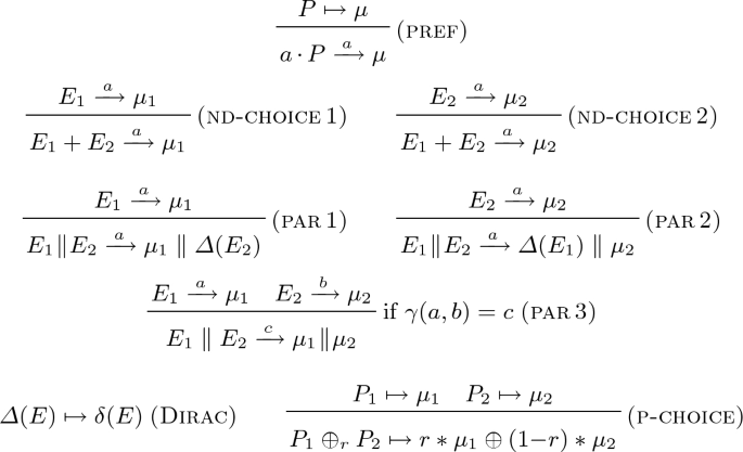
• (a) The transition relations ${\rightarrow } \subseteq \mathcal {E}\times \mathcal {A}\times \textit{Distr}(\mathcal {E})$ and ${\mapsto } \subseteq \mathcal {P}\times \textit{Distr}(\mathcal {E})$ are induced by

  

• (b) The combined transition relation ${\rightarrow } \subseteq \textit{Distr}({\mathcal {E}})\times \mathcal {A}\times \textit{Distr}({\mathcal {E}})$ is such that $\mu \xrightarrow {\,a\,} \mu '$ whenever $\mu = {\textstyle {\bigoplus _{i \mathord {\in } I}}}\, p_i * E_i$, $\mu ' = {\textstyle {\bigoplus _{i \mathord {\in } I}}}\, p_i * \mu '_i$, and for all $i \in I$.

The rules (par 1) to (par 3) above use the parallel operator in combination with distributions. For $\mu _1, \mu _2 \in \textit{Distr}({\mathcal {E}})$ the distribution is such that if and if E is not a parallel composition. See e.g. [26, 28] for similar use of this construction. Note the use of the communication function $\gamma$ in rule (par 3).

The combined transition relation on $\textit{Distr}({\mathcal {E}})$ allows one to split a distribution $\mu$ into $\mu _1 \oplus _r\mu _2$ and to consider transitions of $\mu _1$ and $\mu _2$ for a specific action a independently and combining the resulting distributions. See Example 4.5 in the next section.

Also for the classes of extended processes we provide transition relations.

Definition 3.4

(extended transition relation).

• (a) The transition relations ${\rightarrow } \subseteq \mathcal {E}' \times \mathcal {A}\times \textit{Distr}(\mathcal {E}')$ and ${\mapsto } \subseteq \mathcal {P}' \times \textit{Distr}(\mathcal {E}')$ are induced by the transition rules pref, nd-choice 1,2, par 1,2,3, Dirac, and p-choice together with the transition rules

  

• (b) The combined transition relation ${\rightarrow } \subseteq \textit{Distr}({\mathcal {E}}')\times \mathcal {A}\times \textit{Distr}({\mathcal {E}}')$ is such that whenever $\mu = {\textstyle {\bigoplus _{i \mathord {\in } I}}}\, p_i * E_i$, $\mu ' = {\textstyle {\bigoplus _{i \mathord {\in } I}}}\, p_i * \mu '_i$, and for all $i \in I$.

The machinery of Definition 3.4 is similar to that of Definition 3.3. The additional rules (left) and (sync) capture that in a leftmerge only the component $E_1$ is responsible for determining a possible transition, while for the synchronization operator the synchronization of transitions of both components is required. The former corresponds to rule (par 1), the latter corresponds to rule (par 3).

4 Strong Distribution Bisimulation

In this section the notion of process equivalence of strong distribution bisimulation is presented. Strong distribution bisimulation has been advocated a.o. in [12, 16, 25], called bisimulation, strong probabilistic distribution bisimulation, and strong d-bisimulation, respectively.

Since strong distribution bisimulation deals with distributions rather than states, one has to take a proviso for subsumed behavior. For example, one wants to distinguish the deadlock process $\mathbf{0 }$ and the process $(a \mathop {.}\varDelta ( \mathbf{0 })) \oplus _{1/2} (b \mathop {.}\varDelta ( \mathbf{0 }))$ although both processes do not provide a transition. We follow [25] by introducing the concept of a decomposable relation.

Definition 4.1

(decomposable relation). A symmetric relation $\mathcal {R}$ on $\textit{Distr}({\mathcal {E}})$ is called decomposable iff for all $\mu , \nu \in \textit{Distr}({\mathcal {E}})$ such that $\mu \,{\mathcal {R}}\,\nu$ and $\mu = {\textstyle {\bigoplus _{i \mathord {\in } I}}}\, p_i * \mu _i$ there are $\nu _i \in \textit{Distr}({\mathcal {E}})$, for $i \in I$, such that $\nu = {\textstyle {\bigoplus _{i \mathord {\in } I}}}\, p_i * \nu _i \ \text {and} \ \mu _i \,{\mathcal {R}}\,\nu _i$ for all $i \in I$.

A notion of a decomposable relation on $\textit{Distr}({\mathcal {E}}')$ is defined similarly. Clearly, an arbitrary union of decomposable relations is decomposable again.

The next result is a technical aid to go from comparing distributions to comparing states. It states that every strong distribution bisimulation can be obtained as the convex closure of a relation on states, cf. [13].

Lemma 4.2

Let $\mathcal {R}$ is a decomposable relation on $\textit{Distr}({\mathcal {E}})$. If $\mu \,{\mathcal {R}}\,\nu$, then there are an index set K and non-deterministic processes $E_k, F_k \in \mathcal {E}$ and probabilities $r_k$ for each $k \in K$ such that

Proof

Suppose $\mu \,{\mathcal {R}}\,\nu$ and $\mu = {\textstyle {\bigoplus _{i \mathord {\in } I}}}\, p_i * E_i$. By decomposability of $\mathcal {R}$ we can write $\nu = {\textstyle {\bigoplus _{i \mathord {\in } I}}}\, p_i * \nu _i$ and have $\varDelta (E_i) \,{\mathcal {R}}\,\nu _i$ for suitable $\nu _i \in \textit{Distr}({\mathcal {E}})$, for all $i \in I$. Say, $\nu _i = {\bigoplus _{j \mathord {\in } J_i}}\, q_{ij} * F_{ij}$. By decomposability of $\mathcal {R}$, we have $\varDelta (E_i) = {\bigoplus _{j \mathord {\in } J_i}}\, q_{ij} * \varDelta (E_i)$ and, more importantly, $\varDelta (E_i) \,{\mathcal {R}}\,\varDelta (F_{ij})$ for all $j \in J_i$.

Put $K = \lbrace \,(i,j) \mid i \in I ,\, j \in J_i \, \rbrace$. Put $E'_k = E_i$, $F'_k = F_{ij}$, and $r_k = p_i \cdot q_{ij}$ if $k = (i,j)$. Note, $E'_k \,{\mathcal {R}}\,F'_k$ for $k \in K$. Moreover, we have $\mu = {\textstyle {\bigoplus _{i \mathord {\in } I}}}\, p_i * E_i = {\textstyle {\bigoplus _{i \mathord {\in } I}}}{\bigoplus _{j \mathord {\in } J_i}}\, ( p_i \cdot q_{ij} ) * \varDelta (E_i) = {\bigoplus _{k \mathord {\in } K}}\, r_k * E'_k$, and $\nu = {\textstyle {\bigoplus _{i \mathord {\in } I}}}\, p_i * \nu _i = {\textstyle {\bigoplus _{i \mathord {\in } I}}}\, p_i * ( {\bigoplus _{j \mathord {\in } J_i}}\, q_{ij} * F_{ij} ) = {\bigoplus _{k \mathord {\in } K}}\, r_k * F'_k$ as was to be shown.

The transition systems of Definitions 3.3 and 3.4 incorporate so-called combined transitions. In order to cater for this when dealing with bisimulation we rely on the fact that the convex closure of a decomposable relation is decomposable again.

Lemma 4.3

If a relation $\mathcal {R}$ on $\textit{Distr}({\mathcal {E}})$ is decomposable, then $\mathcal {R}_{ cc }$ the convex closure of $\mathcal {R}$ given by

$$\begin{aligned} \,{\mathcal {R}_{ cc }}\,= \lbrace \,( {\textstyle {\bigoplus _{i \mathord {\in } I}}}\, p_i * \mu _i , {\textstyle {\bigoplus _{i \mathord {\in } I}}}\, p_i * \nu _i ) \mid \forall i \in I :\mu _i \,{\mathcal {R}}\,\nu _i \, \rbrace \end{aligned}$$

is decomposable as well.

Proof

Suppose $\mu = {\textstyle {\bigoplus _{i \mathord {\in } I}}}\, p_i * \mu _i$, $\nu = {\textstyle {\bigoplus _{i \mathord {\in } I}}}\, p_i * \nu _i$ where $\mu _i \,{\mathcal {R}}\,\nu _i$ for $i \in I$. By applying Lemma 4.2 for each pair $\mu _i,\nu _i$ and combining the results we obtain $\mu = {\bigoplus _{j \mathord {\in } J}}\, q_j * E_j$ and $\nu = {\bigoplus _{j \mathord {\in } J}}\, q_j * F_j$ and $\varDelta (E_j) \,{\mathcal {R}}\,\varDelta (F_j)$ for a suitable index set J, processes $E_j, F_j \in \mathcal {E}$ and $q_j > 0$ for $j \in J$.

Now suppose $\mu = {\bigoplus _{k \mathord {\in } K}}\, r_k * \mu '_k$. Then we have $\mu '_k = {\bigoplus _{j \mathord {\in } J}}\, r_{jk} * E_j$ for suitable $r_{jk}$ such that ${\sum _{k {\in } K}}\, r_{jk} \cdot r_k = q_j$. Put $\nu '_k = {\bigoplus _{j \mathord {\in } J}}\, r_{jk} * F_j$. Then we have $\mu '_k \,{\mathcal {R}_{ cc }}\,\nu '_k$ since $\varDelta (E_j) \,{\mathcal {R}}\,\varDelta (F_j)$ for all $j \in J$. Moreover, $\nu = {\bigoplus _{j \mathord {\in } J}}\, q_j * F_j = {\bigoplus _{j \mathord {\in } J}}\, ( {\sum _{k {\in } K}}\, r_{jk} \cdot r_k ) * F_j = {\bigoplus _{k \mathord {\in } K}}\, r_k * ( {\bigoplus _{j \mathord {\in } J}}\, r_{jk} * F_j ) = {\bigoplus _{k \mathord {\in } K}}\, r_k * v'_k$. This proves $\mathcal {R}_{ cc }$ to be decomposable.    $\square$

We are now ready to define the notion of equivalence of processes.

Definition 4.4

(strong distribution bisimulation).

• (a) A decomposable relation $\mathcal {R}\subseteq \textit{Distr}({\mathcal {E}})\times \textit{Distr}({\mathcal {E}})$ is called a strong distribution bisimulation, iff for all $\mu , \nu \in \textit{Distr}({\mathcal {E}})$ such that $\mu \,{\mathcal {R}}\,\nu$ and for some $a \in \mathcal {A}$ and $\mu ' \in \textit{Distr}({\mathcal {E}})$ then and $\mu ' \,{\mathcal {R}}\,\nu '$ for some $\nu ' \in \textit{Distr}({\mathcal {E}})$.

• (b) Strong distribution bisimulation, denoted by , is defined as the largest strong distribution bisimulation on $\textit{Distr}({\mathcal {E}})$.

By the definition of a decomposable relation we have that a strong distribution bisimulation is symmetric. Also note that the relation  on $\textit{Distr}({\mathcal {E}})$ is well-defined. It extends to $\textit{Distr}({\mathcal {E}}')$ straightforwardly.

Example 4.5

Consider the two non-deterministic processes depicted in Fig. 1. We verify that the Dirac distributions $\mu$ and $\nu$ corresponding to these processes, i.e. $\mu = \delta (a \mathop {.}(P \oplus _{1/2} Q) + a \mathop {.}(P \oplus _{1/3} Q))$ for the process on the left and $\nu = \delta (a \mathop {.}(P \oplus _{1/2} Q) + a \mathop {.}(P \oplus _{5/12} Q) + a \mathop {.}(P \oplus _{1/3} Q)))$ for the process on the right, are strongly distribution bisimilar.

Let $\mathcal {R}$ be the relation on $\textit{Distr}({\mathcal {E}})$ given by $\mathcal {R}= \lbrace {\langle {\mu } , {\nu } \rangle , \langle {\nu } , {\mu } \rangle } \rbrace \cup Id _{\textit{Distr}({\mathcal {E}})}$ with $Id _{\textit{Distr}({\mathcal {E}})}$ the identity relation $\lbrace \,\langle {\varrho } , {\varrho } \rangle \mid \varrho \in \textit{Distr}({\mathcal {E}})\, \rbrace$. We claim that $\mathcal {R}$ is a strong distribution bisimulation. It is straightforward to check that $\mathcal {R}$ is decomposable. To see that $\mathcal {R}$ satisfies the transfer condition of Definition 4.4 too, we let $\varrho _P$ and $\varrho _Q$ denote the distributions corresponding to the probabilistic processes P and Q, respectively, and consider the transition . Since $\mu = \frac{1}{2} \mu \oplus \frac{1}{2} \mu$ and both and we obtain from the operational semantics captured by Definition 3.3 . Thus, the distribution $\mu$ exactly matches the transition which is an explicit option of the non-deterministic process on the right of Fig. 1 but not of the other.

Fig. 1.

Two bisimilar processes

Example 4.6

Consider the probabilistic processes P and Q given by

$$\begin{aligned} \begin{array}{rcl} P &{} = &{} \varDelta ( a \mathop {.}\Bigl ( \varDelta (b \mathop {.}\varDelta ( \mathbf{0 })) \oplus _{1/2} \bigl ( \varDelta (c \mathop {.}\varDelta ( \mathbf{0 })) \oplus _{1/2} \varDelta (c \mathop {.}( \varDelta ( \mathbf{0 }) \oplus _{1/2} \varDelta ( \mathbf{0 }) ) \bigr ) \Big ) ) \\ Q &{} = &{} \varDelta ( a \mathop {.}\Bigl ( \bigl ( \varDelta (b \mathop {.}\varDelta ( \mathbf{0 }+ \mathbf{0 })) \oplus _{1/2} \varDelta (b\mathop {.}\varDelta ( \mathbf{0 })) \bigr ) \oplus _{1/2} \varDelta (c \mathop {.}( \varDelta ( \mathbf{0 }) \oplus _{1/2} \varDelta ( \mathbf{0 }) ) \Big ) ) \end{array} \end{aligned}$$

Then we have and for distributions $\mu , \nu \in \textit{Distr}({\mathcal {E}})$ where

$$\begin{aligned} \begin{array}{rcl} \mu &{} = &{} \frac{1}{2} \delta ( b \mathop {.}\varDelta ( \mathbf{0 }) ) \oplus \frac{1}{4} \delta ( c \mathop {.}\varDelta ( \mathbf{0 }) ) \oplus \frac{1}{4} \delta ( c \mathop {.}( \varDelta ( \mathbf{0 }) \oplus _{1/2} \varDelta ( \mathbf{0 }) ) ) \\ \nu &{} = &{} \frac{3}{8} \delta ( b \mathop {.}\varDelta ( \mathbf{0 }+ \mathbf{0 }) ) \oplus \frac{1}{8} \delta ( b \mathop {.}\varDelta ( \mathbf{0 }) ) \oplus \frac{1}{2} \delta ( c \mathop {.}\varDelta ( \mathbf{0 }) ) \end{array} \end{aligned}$$

By decomposability, bisimulation relating $\mu$ and $\nu$ should also relate $\delta ( b \mathop {.}\varDelta ( \mathbf{0 }) )$ to $\delta ( b \mathop {.}\varDelta ( \mathbf{0 }+ \mathbf{0 }) )$ and $\delta ( c \mathop {.}( \varDelta ( \mathbf{0 }) \oplus _{1/2} \varDelta ( \mathbf{0 }) ) )$ to $\delta ( c \mathop {.}\varDelta ( \mathbf{0 }) )$, which requires in turn that $\varDelta ( \mathbf{0 })$ and $\varDelta ( \mathbf{0 }+ \mathbf{0 }) )$ are related. Therefore, we define $\mathcal {R}$ to be the least binary relation on $\textit{Distr}({\mathcal {E}})$ which

• (i) contains the pairs $\langle {P} , {Q} \rangle$, $\langle {\mu } , {\nu } \rangle$, $\langle { \delta ( \mathbf{0 })} , { \delta ( \mathbf{0 }+ \mathbf{0 })} \rangle$, $\langle \delta (b \mathop {.}\varDelta ( \mathbf{0 }) )$, $\delta ( b \mathop {.}$ $\varDelta ( \mathbf{0 }+ \mathbf{0 }))\rangle$, and $\langle { \delta ( c \mathop {.}( \varDelta ( \mathbf{0 }) \oplus _{1/2} \varDelta ( \mathbf{0 })))} , { \delta ( c \mathop {.}\varDelta ( \mathbf{0 }))} \rangle$

• (ii) contains the diagonal $Id _{\mathcal {E}}$

• (iii) is symmetric and convex closed.

It is straightforward to verify that $\mathcal {R}$ is a strong distribution bisimulation relation for P and Q. In particular, because of condition (iii) it is easy to see that $\mathcal {R}$ indeed relates $\mu _1$ and $\nu _1$ as well as $\mu _2$ and $\nu _2$ for the decompositions $\mu = \mu _1 \oplus _{1/2} \mu _2 = \delta (b \mathop {.}\varDelta ( \mathbf{0 })) \oplus _{1/2} ( \frac{1}{2} \delta (c \mathop {.}\varDelta ( \mathbf{0 })) \oplus \frac{1}{2} \delta (c \mathop {.}( \varDelta ( \mathbf{0 }) \oplus _{1/2} \varDelta ( \mathbf{0 })))$ and $\nu = \nu _1 \oplus _{1/2} \nu _2 = ( \frac{3}{4} \delta (b \mathop {.}\varDelta ( \mathbf{0 }+ \mathbf{0 }) \oplus \frac{1}{4} \delta (b \mathop {.}\varDelta ( \mathbf{0 })) \oplus _{1/2} \delta (c \mathop {.}\varDelta ( \mathbf{0 }))$.

The next result states that strong distribution bisimulation is a process equivalence indeed. The congruence property of  is essential for proving the soundness of the equational theory for strong distribution bisimulation that is introduced in the next section.

Theorem 4.7

(congruence). The relation  is an equivalence relation and a congruence on $\mathcal {E}$ and $\mathcal {P}$.

Proof

The proof of being an equivalence relation is straightforward. For congruence we treat the case of the parallel operator.

Suppose $\mathcal {R}_1, \mathcal {R}_2$ are two strong distribution bisimulations. Put

We claim that $\mathcal {R}$ is a strong distribution bisimulation too. By Lemma 4.3 it follows that $\mathcal {R}$ is decomposable. Now suppose $E_1 \,{\mathcal {R}}\,_1 F_1$ and $E_2 \,{\mathcal {R}}\,_2 F_2$ and . We have to show that, for some $\nu \in \textit{Distr}({\mathcal {E}})$, it holds that and $\mu \,{\mathcal {R}}\,\nu$. We distinguish three cases.

Case (i), and : Pick $\nu _1$ such that and $\mu _1 \,{\mathcal {R}}\,_1 \nu _1$. Put . Assume, with help of Lemma 4.2, $\mu _1 = {\textstyle {\bigoplus _{i \mathord {\in } I}}}\, p_1 * E'_i$, $\nu _1 = {\textstyle {\bigoplus _{i \mathord {\in } I}}}\, p_i * F'_i$ and $\varDelta (E'_i) \,{\mathcal {R}}\,_1 \varDelta (F'_i)$ for $i \in I$. Since $\varDelta (E'_i) \,{\mathcal {R}}\,_1 \varDelta (F'_i)$ for $i \in I$ and $\varDelta (E_{2}) \,{\mathcal {R}}\,_{2} \varDelta (F_{2})$ it follows that . Since and we obtain $\mu \,{\mathcal {R}}\,\nu$.

Case (ii), and : Symmetric to case (i).

Case (iii), , , and $\gamma (a_1,a_2) = a$: Suppose $\mu _1 = {\textstyle {\bigoplus _{i \mathord {\in } I}}}\, p_i * E'_i$, $\mu _2 = {\bigoplus _{j \mathord {\in } J}}\, q_j * E''_j$. Since $\varDelta (E_1) \,{\mathcal {R}}\,_1 \varDelta (F_1)$ and $\varDelta (E_2) \,{\mathcal {R}}\,_1 \varDelta (F_2)$ we can find $\nu _1 = {\textstyle {\bigoplus _{i \mathord {\in } I}}}\, p_i * F'_i$, $\nu _2 = {\bigoplus _{j \mathord {\in } J}}\, q_j * F''_j$ in $\textit{Distr}({\mathcal {E}})$ with $\varDelta (E'_i) \,{\mathcal {R}}\,_1 \varDelta (F'_i)$ for $i \in I$ and $\varDelta (E''_j) \,{\mathcal {R}}\,_2 \varDelta (F''_j)$ for $j \in J$. Note for $i \in I$, $j \in J$. Moreover,

from which it follows that $\mu \,{\mathcal {R}}\,\nu$, as was to be shown.    $\square$

5 A Complete Axiomatization

In Table 1 we present the equational theory  that characterizes strong distribution bisimulation for non-deterministic and probabilistic processes. The axioms of  are inspired by the axiomatization of [6] regarding probabilistic choice and that of [8] regarding the synchronization merge. As argued by Moller [30] the availability of the leftmerge  is essential for a finite axiomatization of the merge  itself. This explains why we introduced extended processes incorporating and ${\mathbin {| }}$ in Sect. 3.

Definition 5.1

(theory ). The theory  consists of the axioms listed in Table 1.

Table 1. Axioms for strong distribution bisimulation

The axioms A1 to A4 are as usual. The axioms P1 and P2 express the commutativity and associativity of probabilistic choice, taking into account the probabilities involved. Axiom P3 allows for splitting of a probabilistic process.

The group of processes M, L1 to L3, and S1a to S4 capture the parallel operator  with the help of the auxiliary operators and ${\mathbin {| }}$. Axiom M is an interleaving rule: behavior of a parallel composition  of two processes E and F is either stemming from the process E expressed by , stemming from the process F expressed by , or stemming from the processes E and F synchronizing expresses by $E {\mathbin {| }}F$.

In a leftmerge , by definition, the first step must be taken by the component E. In the extended transition relation of Definition 3.4 only rule (left) applies. This explains axioms L1 and L2. In L2 the expression for $P \in \mathcal {P}$ and $F \in \mathcal {E}$ is defined by and . Axiom L3 expresses that non-deterministic choice distributes over the leftmerge.

Similar considerations apply to axioms S1a to S4 capturing the synchronization operator ${\mathbin {| }}$. Since $E {\mathbin {| }}F$ requires a transition from both operands, deadlock results if either of them doesn’t have such. Synchronization of an a-transition of E and a b-transition of F results in a transition labeled with $\gamma (a,b) \in \mathcal {A}$ as given by the communication function $\gamma$. Non-deterministic choice also distributes over the synchronization operator.

The final axiom C expresses combined behavior. If a non-deterministic process has an a-transition evolving into the probabilistic process P and has an a-transition evolving into the probabilistic process Q, then the non-deterministic process also admits an a-transition evolving into any convex combination of P and Q.

Before moving to completeness of  for  we treat soundness of .

Theorem 5.2

The theory is sound with respect to strong distribution bisimulation for $\mathcal {E}'$ and $\mathcal {P}'$, i.e. for all $E,F \in \mathcal {E}$, if then and for all $P,Q \in \mathcal {P}'$, if then .

Proof

In view of Theorem 4.7 it suffices to show that for each axiom of  the left-hand side and right-hand side are strongly distribution bisimilar. We only cover the case of axiom M.

Pick $E', F' \in \mathcal {E}$ arbitrarily. Define

where ${ Id _{\varDelta }}= \lbrace \,\langle {\varDelta (E)} , {\varDelta (E)} \rangle \mid E \in \mathcal {E}' \, \rbrace$. We have that $\mathcal {R}$ is decomposable, cf. Lemma 4.3.

To see that and match each other, we distinguish six cases: (i) If  because , then and .

(ii) If because , then it holds that and .

(iii) If  because and while , then and .

(iv) If  because , then and .

(v) If because , then it holds that and .

(vi) If  because and while , then and .

It follows that is a strong distribution bisimulation relating and , hence , which was sufficient to show.   $\square$

In the proof of completeness of  we make use of a complexity function c for our inductive argument. We want c to be such that for an axiom $E = F$ or $P = Q$ of AX the weight c(E) or c(P) of the left-hand side is strictly larger in weight than the right-hand side c(F) or c(Q). We will deploy sequences of natural numbers as weights.

Addition on $\mathbb {N}^*$ is defined as element-wise addition. More concretely: (i) $\varepsilon + v = v$, (ii) $u + \varepsilon = u$, (iii) $(n \mathop {.}u) + (m \mathop {.}v) = (n+m) \mathop {.}(u+v)$, for $u,v \in \mathbb {N}^*$ and $n,m \in \mathbb {N}$. The ordering of $\mathbb {N}^*$ is the lexicographic order restricted to sequences of equal length. Thus $n_1 \cdot n_2 \cdot \cdots \cdot n_s < m_1 \cdot m_2 \cdot \cdots \cdot m_t$ iff $s = t$ and for some j, $1 \leqslant j \leqslant s$ it holds that $n_i = m_i$ for $1 \leqslant i < j$ and $n_j < m_j$. Since we only compare sequences of equal length, it holds that < is a well-founded partial order on $\mathbb {N}^*$.

Definition 5.3

(Complexity function). The function $c : \mathcal {E}' \cup \mathcal {P}' \rightarrow \mathbb {N}^*$, assigning a complexity measure to processes, is defined as follows:

Please note, with $\mathbb {N}^*$ the ‘$\mathop {.}$’-operator in the definition of c above denotes concatenation of strings. The complexity function c and the well-foundedness of $\mathbb {N}^*$ are exploited in the technical lemma below.

Lemma 5.4

 

• (a) For each extended non-deterministic process $E' \in \mathcal {E}'$ a basic non-deterministic process $E_0 \in \mathcal {E}_0$ exists such that .

• (b) For each extended probabilistic process $P' \in \mathcal {P}'$ there is a basic probabilistic process $P_0 \in \mathcal {P}_0$ such that .

Proof

Suppose for a context $C[\cdot ]$ and $E_1 = E_2$ an instance of the axiom X of  with $E_1$ its LHS and $E_2$ its RHS. If the axiom X is M, L1-L3, or S1-S4, then it holds that $c(C[E_1]) > c(C[E_2])$. Otherwise, it holds that $c(C[E_1]) = c(C[E_2])$. Moreover, in all cases, it holds that the strings $c(C[E_1])$ and $c(C[E_2])$ are of equal length.

If a process $E \in \mathcal {E}'$ or $P \in \mathcal {P}'$ contains any of the operators , or ${\mathbin {| }}$ then at least one of the axioms M, L1–L3, or S1a–S4 applies, matching its LHS to E or to P, respectively.

If a process $E \in \mathcal {E}'$ or $P \in \mathcal {P}'$ contains none of the operators , or ${\mathbin {| }}$, thus $E \in \mathcal {E}_0$ or $P \in \mathcal {P}_0$, then $c(E) = 0^\ell$ or $c(P) = 0^\ell$ for suitable $\ell \in \mathbb {N}$. This is directly verified by structural induction on E and P: $c( \mathbf{0 }) = 0 = 0^1$, $c(a \mathop {.}P) = 0 \mathop {.}c(P)$, $c(E+F) = c(E)+c(F)$, $c(\varDelta (E)) = 0.c(E)$, $c(P+Q) = c(P)+c(Q)$. Note, a string $0^\ell$ is a minimal element in $\mathbb {N}^*$ for the specific ordering on $\mathbb {N}^*$ introduced above.

It follows that successive elimination of the operators , or ${\mathbin {| }}$ from an extended non-deterministic process $E \in \mathcal {E}'$ by application of the axioms M, L1–L3, or S1–S4, with the LHS of the axiom matching the redex and the RHS yielding the reduct, is a terminating rewrite procedure, with a basic process $E_0 \in \mathcal {E}_0$ as its normal form. The same applies to an extended probabilistic process $P \in \mathcal {P}'$ yielding a basic probabilistic process $P_0 \in \mathcal {P}$.    $\square$

In view of the lemma, relating two bisimilar processes with possible occurrences of  boils down to relating their basic counterparts. However, for this argument to be helpful, we need completeness of , or part of it, for bisimilar basic processes.

Theorem 5.5

The equational theory  consists of the axioms A1–A4, P1–P3, and C. Then it holds that is sound and complete for strong distribution bisimulation for $\mathcal {P}_0$.

As claimed in [6] the proof of Theorem 5.5 is a variation of the standard proof method, cf. [29], and omitted here.

We are now ready to prove completeness of the proposed axiomatization.

Theorem 5.6

The equational theory  is complete with respect to  for $\mathcal {P}$.

Proof

Suppose $P,Q \in \mathcal {P}$ such that . Choose with help of Lemma 5.4 basic processes $P_0, Q_0 \in \mathcal {P}_0$ such that and . Then also by Theorem 4.7. By Theorem 5.5 we obtain . Since is subsumed by  it follows that .    $\square$

We see that the extra complexity in proving Theorem 5.6 and subsequently our resort to the complexity measure c is caused by the mixture  of a probabilistic process and a non-deterministic process in the axiom L2 and the propagation of parallel composition in  in the axiom S2. The general outline however is as established in [8, 29].

6 Concluding Remarks

We studied an elementary process language featuring non-deterministic choice and a parallel operator with synchronous communication on the one hand and probabilistic choice on the other hand. For this language we presented an axiomatization characterizing strong distribution bisimulation and proved soundness and completeness of the proposed set of axioms. The transition system of the language supports so-called combined transitions and treats distributions over non-deterministic processes as its building blocks. In order to support a finite equational theory the processes language was extended with a leftmerge operator and a synchronization operator.

Soundness of the equational theory with respect to strong distribution bisimulation involved, as usual, proving congruence and soundness of the axioms themselves. For completeness, because of the interplay of non-deterministic processes involving the parallel operator, via the leftmerge and synchronization merge, with probabilistic processes, some technical effort was required. The proof, however, stays in line with the standard approach known from the set-up without probabilities.

In [22] a sound and complete equational theory for branching distribution bisimulation, a weak variant of strong distribution bisimulation as treated in the present paper, for a similar process language is proposed. The language however doesn’t include a parallel construct. One may expect that establishing a conservative extension of the theory , thus covering a parallel operator, that captures branching distribution bisimulation will require substantial effort. Not so much for the completeness proof itself, in view of Lemma 5.4, but because of the before-mentioned interplay of non-deterministic and probabilistic processes triggered by the parallel construct. This entanglement requires specific attention when verifying transitivity of the process equivalence at hand and of a congruence result for the parallel operator.

Future work aims at building a framework of a distribution-based notion of process equivalence that allows a complete equational theory, an efficient decision algorithm, and a logical characterization, both with respect to strong bisimulation as well as to a form of weak bisimulation. Especially the construction of a decision algorithm for branching distribution bisimulation attracts our attention. A decision algorithm for weak distribution bisimulation is proposed in [16]. A rather efficient algorithm for strong probabilistic bisimulation has been presented in [21], building on the the work of [5] and [35]. We hope to be able to extend the approach of [21] to cater for strong distribution bisimulation first.

In the long run we aim to build a probabilistic extension of the mCRL2 toolset [10] (also see www.mcrl2.org) of which a modest part has been realized as yet [23]. Possibly the completeness result presented in the current paper will provide a similar building block for our framework as the completeness result of [20], reworked in [19], does for ACTL, the action-based version of CTL, which is underpinning the KandISTI tool family [7] developed at CNR/ISTI.

References

Andova, S., Baeten, J.C.M., Willemse, T.A.C.: A complete axiomatisation of branching bisimulation for probabilistic systems with an application in protocol verification. In: Baier, C., Hermanns, H. (eds.) CONCUR 2006. LNCS, vol. 4137, pp. 327–342. Springer, Heidelberg (2006). https://doi.org/10.1007/11817949_22
Andova, S., Willemse, T.A.C.: Branching bisimulation for probabilistic systems: characteristics and decidability. Theor. Comput. Sci. 356, 325–355 (2006)
Baeten, J.C.M., Basten, T., Reniers, M.A.: Process Algebra: Equational Theories of Communicating Processes. Cambridge Tracts in Theoretical Computer Science, vol. 50. CUP, Cambridge (2010)
Baeten, J.C.M., Bergstra, J.A., Smolka, S.A.: Axiomatizing probabilistic processes: ACP with generative probabilities. Inf. Comput. 121(2), 234–255 (1995)
Baier, C., Engelen, B., Majster-Cederbaum, M.E.: Deciding bisimilarity and similarity for probabilistic processes. J. Comput. Syst. Sci. 60, 187–231 (2000)
Bandini, E., Segala, R.: Axiomatizations for probabilistic bisimulation. In: Orejas, F., Spirakis, P.G., van Leeuwen, J. (eds.) ICALP 2001. LNCS, vol. 2076, pp. 370–381. Springer, Heidelberg (2001). https://doi.org/10.1007/3-540-48224-5_31
ter Beek, M.H., Gnesi, S., Mazzanti, F.: From EU projects to a family of model checkers. In: De Nicola, R., Hennicker, R. (eds.) Software, Services, and Systems. LNCS, vol. 8950, pp. 312–328. Springer, Cham (2015). https://doi.org/10.1007/978-3-319-15545-6_20
Bergstra, J.A., Klop, J.W.: Process algebra for synchronous communication. Inf. Control 60(1–3), 109–137 (1984)
Bernardo, M., Gorrieri, R.: Extended Markovian process algebra. In: Montanari, U., Sassone, V. (eds.) CONCUR 1996. LNCS, vol. 1119, pp. 315–330. Springer, Heidelberg (1996). https://doi.org/10.1007/3-540-61604-7_63
Bunte, O., et al.: The mCRL2 toolset for analysing concurrent systems. In: Vojnar, T., Zhang, L. (eds.) TACAS 2019. LNCS, vol. 11428, pp. 21–39. Springer, Cham (2019). https://doi.org/10.1007/978-3-030-17465-1_2
Crafa, S., Ranzato, F.: Logical characterizations of behavioral relations on transition systems of probability distributions. ACM Trans. Comput. Logic 16(1), 2:1–2:24 (2014)
Deng, Y., Hennessy, M.: On the semantics of Markov automata. In: Aceto, L., Henzinger, M., Sgall, J. (eds.) ICALP 2011. LNCS, vol. 6756, pp. 307–318. Springer, Heidelberg (2011). https://doi.org/10.1007/978-3-642-22012-8_24
Deng, Y., Hennessy, M.: On the semantics of Markov automata. Inf. Comput. 222, 139–168 (2013)
Deng, Y., Palamidessi, C.: Axiomatizations for probabilistic finite-state behaviors. Theor. Comput. Sci. 373, 92–114 (2007)
Deng, Y., Palamidessi, C., Pang, J.: Compositional reasoning for probabilistic finite-state behaviors. In: Middeldorp, A., van Oostrom, V., van Raamsdonk, F., de Vrijer, R. (eds.) Processes, Terms and Cycles: Steps on the Road to Infinity. LNCS, vol. 3838, pp. 309–337. Springer, Heidelberg (2005). https://doi.org/10.1007/11601548_17
Eisentraut, C., Hermanns, H., Krämer, J., Turrini, A., Zhang, L.: Deciding bisimilarities on distributions. In: Joshi, K., Siegle, M., Stoelinga, M., D’Argenio, P.R. (eds.) QEST 2013. LNCS, vol. 8054, pp. 72–88. Springer, Heidelberg (2013). https://doi.org/10.1007/978-3-642-40196-1_6
Fischer, N., van Glabbeek, R.: Axiomatising infinitary probabilistic weak bisimilarity of finite-state behaviours. J. Log. Algebr. Methods Program. 102, 64–102 (2019)
Giacalone, A., Jou, C.-C., Smolka, S.A.: Algebraic reasoning for probabilistic concurrent systems. In: Broy, M. (ed.) Proceedings of IFIP WG 2.2 & 2.3 Working Conference on Programming Concepts and Methods, pp. 443–458 (1990)
Gnesi, S., ter Beek, M.H.: From the archives of the formal methods and tools lab. In: Boreale, M., Corradini, F., Loreti, M., Pugliese, R. (eds.) Models, Languages, and Tools for Concurrent and Distributed Programming. LNCS, vol. 11665, pp. 219–235. Springer, Cham (2019). https://doi.org/10.1007/978-3-030-21485-2_13
Gnesi, S., Larosa, S.: A sound and complete axiom system for the logic ACTL. In: De Santis, A. (ed.) Proceedings of ICTCS 1995, Ravello, 9–11 November 1995, pp. 291–306 (1995)
Groote, J.F., Rivera Verduzco, H.J., de Vink, E.P.: An efficient algorithm to determine probabilistic bisimulation. Algorithms 11(9), 131–1-22 (2018)
Groote, J.F., de Vink, E.P.: A complete axiomatization of branching bisimulation for a simple process language with probabilistic choice, Submitted
Groote, J.F., de Vink, E.P.: Problem solving using process algebra considered insightful. In: Katoen, J.-P., Langerak, R., Rensink, A. (eds.) ModelEd, TestEd, TrustEd. LNCS, vol. 10500, pp. 48–63. Springer, Cham (2017). https://doi.org/10.1007/978-3-319-68270-9_3
Hansson, H., Jonsson, B.: A calculus for communicating systems with time and probabilities. In: Proceedings of RTSS 1990, pp. 278–287. IEEE (1990)
Hennessy, M.: Exploring probabilistic bisimulations, part I. Formal Aspects Comput. 24, 749–768 (2012)
Hillston, J.: A compositional approach to performance modelling. Ph.D thesis, University of Edinburgh (1994)
Larsen, K.G., Skou, A.: Bisimulation through probabilistic testing. Inf. Comput. 94, 1–28 (1991)
Latella, D., Massink, M., de Vink, E.P.: Bisimulation of labelled state-to-function transition systems coalgebraically. Log. Methods Comput. Sci. 11(4) (2015). https://doi.org/10.2168/LMCS-11(4:16)2015, https://lmcs.episciences.org/1617
Milner, R.: Communication and Concurrency. Prentice Hall, Englewood Cliffs (1989)
Moller, F.: The importance of the left merge operator in process algebras. In: Paterson, M.S. (ed.) ICALP 1990. LNCS, vol. 443, pp. 752–764. Springer, Heidelberg (1990). https://doi.org/10.1007/BFb0032072
Parma, A., Segala, R.: Logical characterizations of bisimulations for discrete probabilistic systems. In: Seidl, H. (ed.) FoSSaCS 2007. LNCS, vol. 4423, pp. 287–301. Springer, Heidelberg (2007). https://doi.org/10.1007/978-3-540-71389-0_21
Segala, R.: Modeling and Verification of Randomzied Distributed Real-Time Systems. Ph.D thesis, MIT (1995). Technical report MIT/LCS/TR-676
Segala, R., Lynch, N.: Probabilistic simulations for probabilistic processes. In: Jonsson, B., Parrow, J. (eds.) CONCUR 1994. LNCS, vol. 836, pp. 481–496. Springer, Heidelberg (1994). https://doi.org/10.1007/978-3-540-48654-1_35
Stark, E.W., Smolka, S.A.: A complete axiom system for finite-state probabilistic processes. In: Plotkin, G.D., Stirling, C., Tofte, M. (eds.) Proof, Language, and Interaction, Essays in Honour of Robin Milner, pp. 571–596. The MIT Press (2000)
Valmari, A.: Simple bisimilarity minimization in O(mlogn) time. Fundamenta Informaticae 105(3), 319–339 (2010)
Acknowledgement
JFG acknowledges the mutual inspiration of the development teams of mCRL2 and KandISTI. A nice example is the inclusion of the LTS minimization algorithm as provided in the mCRL2 toolset which has been incorporated in the KandISTI family members UMC and FMC. Also the attention for model checking of variability and software product lines with the mCRL2 toolset is such an example. EV acknowledges the warm hospitality of Stefania Gnesi and her research group at the CNR in Pisa at various occasions and the many pasti accoglienti shared together.
Author information
Authors and Affiliations
Corresponding author
Editor information
Editors and Affiliations
Rights and permissions
Copyright information
© 2019 Springer Nature Switzerland AG
About this chapter
Cite this chapter
Groote, J.F., de Vink, E.P. (2019). An Axiomatization of Strong Distribution Bisimulation for a Language with a Parallel Operator and Probabilistic Choice. In: ter Beek, M., Fantechi, A., Semini, L. (eds) From Software Engineering to Formal Methods and Tools, and Back. Lecture Notes in Computer Science(), vol 11865. Springer, Cham. https://doi.org/10.1007/978-3-030-30985-5_26
Download citation
DOI: https://doi.org/10.1007/978-3-030-30985-5_26
Published:
Publisher Name: Springer, Cham
Print ISBN: 978-3-030-30984-8
Online ISBN: 978-3-030-30985-5
eBook Packages: Computer ScienceComputer Science (R0)