
Abstract
This tutorial introduces the basic ideas of software specification and verification, which are important techniques for assuring the quality of software and eliminating common kinds of errors such as buffer overflow. The tutorial takes a practical hands-on approach using the Whiley language and its verifying compiler. This verifying compiler uses an automated proof engine to try to prove that the code will execute without errors and will satisfy its specifications. Each section of the tutorial includes exercises that can be checked using the online Whiley Labs website.
Access provided by Autonomous University of Puebla. Download chapter PDF
1 Background
In our modern world, software is a trusted part of many aspects of our lives. Unfortunately, the impact and significance of software failures has increased dramatically over the last decade [15, 40]. A study into software problems between 1980–2012 concluded “About once per month on average, the news reports death, physical harm, or threatened access to food or shelter due partly to software problems” [40]. One study found that more than one-third of water, gas and electricity failures were caused by software faults [53]. A modern automobile has an estimated 100M lines of computer code [14], which makes them vulnerable to software faults. In 2003, a blackout caused by software failure lasted 31 hours and affected around 50 million people in the US/Canada [58]. In 2015, a software bug was discovered in the Boeing 787 despite over a decade of development by that point and \(\approx \)300 planes in operation [35]. To mitigate the risk of catastrophic mid-flight failure, the US Federal Aviation Administration issued a directive, instructing airlines to reboot the control units on all Boeing 787s at least once every 248 days. Other similar examples include: the Therac-25 computer-operated X-ray machine, which gave lethal doses to patients [47]; the 1991 Patriot missile which hit a barracks, killing several people [32]; and the Ariane 5 rocket which exploded shortly after launch, costing the European Space Agency an estimated $500 million [1].
Software is also important for our privacy and security. Black hats are hackers who break into computer systems for criminal purposes, such as stealing credit card numbers. Many attacks on computer systems are enabled because of hidden software bugs. One such example was the infamous Heartbleed bug disclosed in 2014 [10, 25]. This was a relatively simple software bug (in fact, a buffer overrun) found in the widely used OpenSSL cryptography library. There was concern across the internet for several reasons: firstly, a large number of people were affected (at the time, around half a million secure web servers were believed to be vulnerable); secondly, OpenSSL was an open source project but the bug had gone unnoticed for over two years. Joseph Steinberg of Forbes wrote, “Some might argue that [Heartbleed] is the worst vulnerability found (at least in terms of its potential impact) since commercial traffic began to flow on the Internet” [55].
Given the woeful state of much of the software we rely on every day, one might ask what can we as computer scientists do about it? Of course, we want to ensure that software is correct. But how? To answer this, we need to go back and rethink what software development is. When we write a program, we have in mind some idea of what this means. When we have finished our program, we might run it to see whether it appears to do the right thing. However, as anyone who has ever written a program will know: this is not always enough! Even if our program appears to work after a few tests, there is still a good chance it will go wrong for other inputs we have not yet tried. The question is: how can we be sure our program is correct?
2 Specification and Verification
In trying to determine whether our program is correct, our first goal is to state precisely what it should do. In writing our program, we may not have had a clear idea of this from the outset. Therefore, we need to determine a specification for our program. This is a precise description of what the program should and should not do. Only with this can we begin to consider whether or not our program actually does the right thing. If we have used a modern programming language, such as Java, C# or C++, then we are already familiar with this idea. These languages require a limited specification be given for functions in the form of types. That is, when writing a function in these languages we must specify the permitted type of each parameter and the return. These types put requirements on our code and ensure that certain errors are impossible. For example, when calling a function we must ensure that the argument values we give have the correct type. If we fail to do this, the compiler will complain with an error message describing the problem, which we must fix before the program will compile.
Software verification is the process of checking that a program meets its specification. In this chapter we adopt a specific approach referred to as automated software verification. This is where a tool is used to automatically check whether a function meets its specification or not. This is very similar to the way that compilers for languages like Java check that types are used correctly. The tool we choose for this is a programming language called Whiley [52], which allows us to write specifications for our functions, and provides a special compiler which will attempt to check them for us automatically.
This chapter gives an introduction to software verification using Whiley. Whiley is not the only tool we could have chosen, but it has been successfully used for several years to teach software verification to undergraduate software engineering students. Other tools such as Spark/ADA, Dafny, Spec#, ESC/Java provide similar functionality and could also be used with varying degrees of success.
3 Introduction to Whiley
The Whiley programming language has been in active development since 2009. The language was designed specifically to help the programmer eliminate bugs from his/her software. The key feature is that Whiley allows programmers to write specifications for their functions, which are then checked by the compiler. For example, here is the specification for the
 function which returns the maximum of two integers:

Here, we see our first piece of Whiley code. This declares a function called max which accepts two integers
 and
and
 , and returns an integer
 . The body of the function simply compares the two parameters and returns the largest. The two
 clauses form the function’s post-condition, which is a guarantee made to any caller of this function. In this case, the max function guarantees to return one of the two parameters, and that the return will be as large as both of them. In plain English, this means it will return the maximum of the two parameter values.
3.1 Whiley Syntax
Whilst a full introduction to the Whiley language is beyond this tutorial, we provide here a few notes relevant to the remainder. A more complete description can be found elsewhere [51].
-
Indentation Syntax. Like Python, Whiley uses indentation to identify block structure. So a colon on the end of a line indicates that a more heavily indented block of statements must follow.
-
Equality. Like many popular programming languages, Whiley uses a double equals for equality and a single equals for assignment. But in mathematics and logic, it is usual to use a single equality sign for equality. In this paper, we shall use the Whiley double-equals notation within Whiley programs (generally typeset in rectangles) and within statements S in the middle of Hoare triples \(\{P\}\;S\;\{Q\}\), but just a single-equals for equality when we are writing logic or maths.
-
Arrays. The size of an array
 is written as
 in Whiley, and array indexes range from
 upto
upto
 .
. -
Quantifiers. In Whiley, quantifiers are written over finite integer ranges. For example, a universal quantifier
 ranges from the lower bound
 up to (but not including) the upper bound
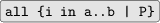
 . For example, we can specify that every item in an array
 is positive with
 .
.
 is written as
 in Whiley, and array indexes range from
 upto
upto
 .
. ranges from the lower bound
 up to (but not including) the upper bound
 . For example, we can specify that every item in an array
 is positive with
 .
.When verification is enabled the Whiley compiler will check that every function meets its specification. For our
 function, this means it will check that the body of the function guarantees to return a value which meets the function’s postcondition. To do this, it will explore the two execution paths of the function and check each one separately. If it finds a path which does not meet the postcondition, the compiler will report an error. In this case, the
 function above is implemented correctly and so it will find no errors. The advantage of providing specifications is that they can help uncover bugs and other, more serious, problems earlier in the development cycle. This leads to software which is both more reliable and more easily maintained (since the specifications provide important documentation).
4 Writing Specifications
Specifying a program in Whiley consists of at least two separate activities. Firstly, we provide appropriate specifications (called invariants) for any data types we have defined (we will discuss this further in Sect. 4.4). Secondly, we provide specifications in the form of preconditions and postconditions for any functions or methods defined—which may involve defining additional data types and properties. In doing this, we must acknowledge that precisely describing a program’s behaviour is extremely challenging and, oftentimes, we want only to specify some important aspect of its permitted behaviour. This can give us many of the benefits from specification without all of the costs.
4.1 Specifications as Contracts
A specification is a contract between two parties: the client and supplier. The client represents the person(s) using a given function (or method or program), whilst the supplier is the person(s) who implemented it. The specification ties the inputs to the outputs in two ways:
-
Inputs. The specification states what is required of the inputs for the function to behave correctly. The client is responsible for ensuring the correct inputs are given. If an incorrect input is given, the contract is broken and the function may do something unexpected.
-
Outputs. The specification states what outputs must be ensured by a correctly behaving function. The supplier is responsible for ensuring all outputs meet the specification, assuming that correct inputs were provided.
From this, we can see that both parties in the contract have obligations they must meet. This also allows us to think about blame. That is, when something goes wrong, who is responsible? If the inputs to our function were incorrect according to the specification, we can blame the client. On the other hand if the inputs were correct, but the outputs were not, we can blame the supplier.
An interesting question arises about who the client and supplier are, exactly. A common scenario is where they are different people. For example, the supplier has written a library that the client is using. However, this need not be the case and, in fact, they can be the same person. For example, consider a program with one function
 that calls another
 , both of which were written by the same person. In this case, that person acts as both client and supplier: first as a client of
 (i.e. because their function
 calls
calls
 and relies on its specification); second, they are a supplier of
 because they implemented it and are responsible for it meeting its specification. Finally, we note the special case of the top level function of a program (e.g.
 )) which is called the language runtime. If this function has a precondition, then it is the responsibility of the runtime to ensure this is met. A good example of this is when an array of
 s are passed to represent command-line arguments. In such case, there may be a precondition that the array is not
 .
.
Example. As an example, let us consider a function for finding the maximum value from an array of integers. Here is an informal specification for this function:

We have specified our function above using comments to document: firstly, the requirements needed for the inputs—that the array must have at least one element; and, secondly, the expectations about the outputs—that it returns the largest element in the array. Thus, we could not expect the call
 to operate correctly; likewise, if the call
 returned
 we would say the implementation was incorrect. \(\blacksquare \)
4.2 Specifying Functions
To specify a function or method in Whiley we must provide an appropriate precondition and postcondition. A precondition is a condition over the input parameters of a function that is required to be true when the function is called. The body of the function can use this to make assumptions about the possible values of the parameters. Likewise, a postcondition is a condition over the return values of a function that is required to be true after the function body is executed.
Example. As a very simple example, consider the following specification for our function which finds the maximum value from an array of integers:

Here, the
 clause gives the function’s precondition, whilst the
 clauses give its postcondition. This specification is largely the same as that given informally using comments before. However, we regard this specification as being formal because, for any set of inputs and outputs, we can calculate precisely whether the inputs or outputs satsify these specifications.
For example, consider the call
 . We can say that the inputs to this call are incorrect, because
 evaluates to
 . For the informal version given above, we cannot easily evaluate the English comments to determine whether they were met or not. Instead, we rely on our human judgement for this—but, unfortunately, this can easily be wrong! \(\blacksquare \)
When specifying a function in Whiley, the
 clause(s) may only refer to the input parameters, whilst the
 clause(s) may also refer to the return parameters. Note, however, that the
 clause(s) always refers to the values of the parameters on entry to the function, not those which might hold at the end.

4.3 Contractual Obligations
The main benefit of adding specification clauses (
 and
and
 ) to a function is that it gives us a precise contract that acts as an agreement between the client and the supplier of the function. We can now be more precise about the obligations and benefits for both parties.
-
The client, who calls the function, must make certain that every input value satisfies the
 conditions (Obligation); and, can assume every output of the function satisfies the
 conditions (Benefit).
 -
The supplier, who implements the function, must ensure all returned values satisfy the
 conditions (Obligation); but, may assume that every input will satisfy the
 conditions (Benefit).
 conditions (Obligation); and, can assume every output of the function satisfies the
 conditions (Benefit).
 conditions (Obligation); but, may assume that every input will satisfy the
 conditions (Benefit).
In both cases, the Whiley verifying compiler will check these obligations and display an error message such as “postcondition may not be satisfied” if its automatic prover cannot prove that the obligation is satisfied. This could mean either that:
-
the proof obligation is false, so the code is incorrect; or
-
the automatic prover is not powerful enough to prove the obligation.
In general, software correctness proofs are undecidable, especially when they involve non-trivial multiplications or other non-linear functions, so the automatic prover has a timeout (typically 10 s) after which it reports that it cannot prove the proof obligation. So when the Whiley compiler reports an error, it could mean an error in the code, or just that something is too hard to prove automatically. To help decide which is the case, one can ask the Whiley verifier to generate a counter-example. If it is able to generate counter-example values, then this can be inspected to see why the proof obligation is false - it could be due to an error in the code or in the specification. If the Whiley verifier cannot find any counter-example values, then it is possible that the proof obligation is too complex for the verifier to be able to prove within its timeout limit. In this case one can: increase the timeout; or, simplify the code and specifications to make the proof obligation more obvious; or, mark this proof obligation as needing further inspection and verification by humans.


4.4 Specifying Data Types
In Whiley, a data type is simply a set of values. Practically, the usual structured types are supported (arrays and records), as well as various primitive types such as integer and boolean. In addition, the Whiley type system allows users to specify data invariants as part of a type definition. For example, we could define a type called
 that is the strictly positive integers, or a type
 that can range only from \(0 \ldots 100\). The following example shows how we can define a
 type that is restricted to only allow non-empty rectangles.


5 Verifying Loop-Free Code
In this section we will practice verifying simple non-looping programs that contain just: assignment statements, variable declarations, if-else conditionals, return statements, and assertions. A key challenge here lies in understanding how the automated verification tool works. To help, we will introduce some theory—called Hoare logic—which provides a mathematical background for verification [34]. Whilst the verification tools can be used without understanding all the details of this theory, it is recommended to work through Sects. 5.1 to 5.4 to get a deeper understanding.
5.1 Motivating Example
We shall start with a brain teaser. Here is some Whiley code (adapted from an example by Back and von Wright [4, page 97–98]) that does some kind of transformation of two values. Try to work out what it does, and write a specification of its input-output behavior by completing the
 predicate.

This example shows that it can be quite complex to reason about a sequence of assignments. It is not always obvious what state the variables should be in between two statements. In fact, the specification of this code is remarkably simple and this will become apparently shortly. But this probably was not obvious from the rather convoluted code, which was designed to swap two variables (and double one of them) without using any temporary storage – such code was useful when embedded computers had extremely limited memory, but is rarely needed these days.
Software verification tools can sometimes immediately verify our code, even when it does have a complex sequence of assignments like this. But when there is a problem, we will sometimes need to ‘debug’ our program or our verification, step by step, which requires that we understand the intermediate states. So we need intermediate predicates between statements to say what should be true at that point. Whiley provides two kinds of statements which can help:
-
 to check if
 is true at that point. The verifier will attempt to prove that
 is satisfied at that point and will give an error if it is not provable. Adding assertions makes the verifier work a little harder, but will never destroy the soundness of the verification.
 -
 to add an (unproven) assumption. The verifier will not attempt to prove
 , but will simply assume that it is true at that point, and will use it to help verify subsequent proof obligations. Assumptions can be useful for performing ‘what if’ experiments with the verifier, or for helping the verifier to overcome difficult proofs that it cannot do automatically. However, assumptions allow one to override the usual verification process, so care must be taken not to introduce unsound verifications by adding incorrect assumptions.
 to check if
 is true at that point. The verifier will attempt to prove that
 is satisfied at that point and will give an error if it is not provable. Adding assertions makes the verifier work a little harder, but will never destroy the soundness of the verification.
 to add an (unproven) assumption. The verifier will not attempt to prove
 , but will simply assume that it is true at that point, and will use it to help verify subsequent proof obligations. Assumptions can be useful for performing ‘what if’ experiments with the verifier, or for helping the verifier to overcome difficult proofs that it cannot do automatically. However, assumptions allow one to override the usual verification process, so care must be taken not to introduce unsound verifications by adding incorrect assumptions.
By inserting assertions and assumptions at various points in our program, we can check our understanding of what should be true and, if necessary, can prove one scenario at a time. For example, we could use
 statements to focus on particular input values such as \(x==10\) and \(y==11\), and an
 statement to check that we have done the correct calculation for those values.

But how can we find, or design, these intermediate assertions? This is where Hoare logic comes in. But, before we get to that, here is the solution for our brain teaser.

Now let’s investigate the three ways that we can calculate intermediate assertions for complex sequences of code.
5.2 Hoare Logic
Hoare Logic [34] is a well-known system for proving the correctness of programs. Figure 1 presents Hoare Logic rules for the basic statements in Whiley. Note that \(p[e/x]\) means replace all free occurrences of the variable x in p by the expression e. Unlike Hoare’s original logic, Fig. 1 includes
 and
and
 statements, and loops have explicit loop invariants.
The rules are presented in terms of correctness assertions (also known as Hoare triples of the form:  , where \(\mathtt{p}\) is a precondition, \(\mathtt{s}\) is a Whiley statement, and \(\mathtt{q}\) is a postcondition. A Hoare triple is true if whenever the precondition is true, then executing the statement establishes the postcondition. For example, consider the following Hoare triple:
Here we see that, if \(\mathtt{x\ge 0}\) holds immediately before the assignment then, as expected, it follows that \(\mathtt{x > 0}\) holds afterwards. However, whilst this is intuitively true, it is not so obvious how this triple satisfies the rules of Fig. 1. For example, as presented it does not immediately satisfy H-Assign. However, rewriting the triple is helpful here:
The above triple clearly satisfies H-Assign since \((x>0) [x+1/x]\) simplifies to \(x+1>0\), which is the same as our precondition. Furthermore, we can obtain the original triple from this triple via H-Consequence (i.e. since \(x+1>0\implies x\ge 0\)).
5.3 Calculating Backwards Through Assignments
The rules of Fig. 1 naturally give rise to an approach where we calculate preconditions from postconditions. Whilst this may seem unnatural at times, it is rather convenient. We can take this further and consider the weakest precondition that can be calculated. This is the weakest condition \(\mathtt{p}\) that guarantees that if it is the case that statement \(\mathtt{s}\) terminates, then the final state will satisfy \(\mathtt{q}\). The rule H-Assign for assignment statements demonstrates this most clearly. Consider the following:
To apply rule H-Assign here, we simply substitute all occurrences of \(\mathtt{x}\) in the postcondition with \(\mathtt{y+1}\) (i.e. the expression being assigned) to give:

Extended rules of Hoare Logic.
At this point, we have a simple mechanism for calculating the weakest precondition for a straight-line sequence of statements.

Variable Versions. Since Whiley is an imperative language, it permits variables to be assigned different values at different points. Whilst the rules of Hoare logic accomodate this quite well, there are some limitations. In particular, we often want to compare the state of a variable before and after a given statement.
The following illustrates this:

We can express the above program as a straight line sequence of Hoare triples where the
 is represented as
 (i.e it is treated as an assignment to the return variable):
However, there must be a problem since the intermediate assertion \(\mathtt{x > x}\) is clearly false. So what went wrong? The problem lies in our formulation of the postcondition in the final assertion. Specifically, in the final assertion, \(\mathtt{x}\) refers to the value of variable \(\mathtt{x}\) at that point. However, in the
 clause,
 refers to the value of
 on entry.
In order to refer to the value of a variable on entry, we can use a special version of it. In this case, let \(\mathtt{x_0}\) refer to the value of variable \(\mathtt{x}\) on entry to the function. Then, we can update our Hoare triples as follows:
By assuming that \(\mathtt{x = x_0}\) on entry to the function, we can see the weakest precondition calculated we’ve calculated above is satisfied.
5.4 Calculating Forwards Through Assignments
An alternative approach is to propagate predicates forward through the program. For a given precondition, and a statement s, we want to find the strongest postcondition that will be true after s terminates. This turns out to be a little more challenging than calculating weakest preconditions. Consider this program:
From the precondition to this statement, one can infer that \(\mathtt{y}\) is non-negative. But, how to update this and produce a sensible postcondition which retains this information? The problem is that, by assigning to \(\mathtt{x}\), we are losing information about its original value and relationship with \(\mathtt{y}\). For example, substituting \(\mathtt{x}\) for \(\mathtt{1}\) as we did before gives \(\mathtt{0 \le 1 \le y}\) which is certainly incorrect, as this now implies \(\mathtt{y}\) cannot be zero (which was permitted before). The solution is to employ Floyd’s rule for assignments [30]:
This introduces a new variable \(\mathtt{v}\) to represent the value of \(\mathtt{x}\) before the assignment and, hence, provide a mechanism for retaining all facts known beforehand. For above example, this looks like:
With this postcondition, we retain the ability to infer that \(\mathtt{y}\) is non-negative. Unfortunately, the postcondition seems more complex. To simplify this, we can employ the idea of variable versioning from before:
Here, \(\mathtt{x_0}\) represents the value of \(\mathtt{x}\) before the assignment. We are simply giving a name (\(\mathtt{x_0}\)) to the value that Floyd’s Rule claims to exist. Technically this is called ‘skolemization’. Observe that, with multiple assignments to the same variable, we simply increment the subscript of that variable each time it appears on the left-hand side of an assignment statement. The following illustrates this:

This approach of strongest postconditions with variable versions is essentially how the Whiley verifier analyzes each path through the Whiley code. In fact, when looking at a counter-example from the verifier for a proof that fails (for whatever reason), one will sometimes see numbered versions of some variables, referring to their intermediate values. One reason for using this strongest postcondition approach in preference to the weakest precondition approach is that the strongest postcondition approach typically generates multiple smaller proof obligations rather than one large proof obligation, which helps to make error messages more precise and helpful.
5.5 Reasoning About Control-Flow
Reasoning about conditional code, such as if-else statements, is similar to reasoning about a single sequence of code, except that we now have two or more possible execution sequences. So we must reason about each possible sequence. To do this, we use the following three principles:
-
Within the true branch the condition is known to hold;
-
Within the false branch the condition is known to not hold;
-
Knowledge from each branch can be combined afterwards using disjunction.
The following illustrates what assertions are true at each point in the code. Note how the assertion after the whole if-else block is simply the disjunction of both branches, and from this disjunction we are able to prove the desired postcondition \(z \ge 0\).

A return statement terminates a function and returns to the calling function. Since execution does not continue in the function after the return, our reasoning about sequences of code also stops at each return statement. At that point, we must prove that the postcondition of the whole function is satisfied. The following example illustrates this:


A recursive function for summing an array of integers
5.6 Reasoning About Expressions
Our next example (see Fig. 2) illustrates a more complex function example that uses conditionals and recursion to sum an array of integers. Note that variable declarations in Whiley are typed like in Java and C, so \(\mathtt{int\;x\; = \; \ldots }\) declares and initializes the variable \(\mathtt{x}\).
One issue that arises in this example is that whenever the code indexes into an array, we need to check that the index is a valid one. Checks like this ensure that buffer overflows can never occur, thereby eliminating a major cause of security vulnerabilities. To ensure that the array access in line 14 is valid, we must prove that at that point the index
 is within bounds. This introduces the following proof obligation—or verification condition—for our program (we use a bold implies to clearly separate the assumptions of the proof obligation from the conclusions):

The Whiley verifier can easily prove this verification condition holds true and, hence, that the array access is within bounds.
More generally, many inbuilt functions have preconditions that we need to check. For example, the division operator \(\mathtt{a/b}\) is only valid when \(\mathtt{b \ne 0}\). And user-defined functions have preconditions, which must be satisfied when they are invoked, so the verifier must generate verification conditions to check their arguments. Here is a list of the verification conditions that Whiley generates and checks to verify code:
-
1.
Before every function call, the function’s precondition is true;
-
2.
Before every array access, \(\mathtt{arr[i]}\), the index \(\mathtt{i}\) is within bounds;
-
3.
Before every array generator, \(\mathtt{[v; n]}\), the size \(\mathtt{n}\) is non-negative;
-
4.
Before every integer division \(\mathtt{a/b}\), it is true that \(\mathtt{b \ne 0}\);
-
5.
Every assert statement is true;
-
6.
in assignment statements, each right-hand-side result satisfies the type constraints of the corresponding left-hand-side variable;
-
7.
At each return, the ensures conditions are true.
These conditions apply to the recursive invocation of \(\mathtt{sum(\ldots )}\) on Line 16 as well. We must prove that the precondition of \(\mathtt{sum(\ldots )}\) is satisfied just before it is called. In this case this means proving:
-
\(\mathtt{0 \le i \le |items|\wedge i\ne |items| \;\mathbf implies\mathtt \;0 < i\!+\!1\le |items|}\)
-

 .
.

 .
.Note that if we wanted to prove termination, to ensure that this function does not go into infinite recursion, we would also need to define a decreasing variant expression and prove that each recursive call strictly decreases the value of that expression towards zero. However, the current version of Whiley only proves partial correctness, so does not generate proof obligations to ensure termination. This may be added in the future.
5.7 Reasoning About Function Calls
Correctly reasoning about code which calls another function can be subtle. In our recursive
 example we glossed over this by simply applying the postcondition for
 directly. Sometimes we need to reason more carefully. It is important to understand that the verifier never considers the body of functions being called, only their specification. This makes the verification modular. Consider the following simple function:

This is the well-known identity function which simply returns its argument untouched. However, even with this simple function, it is easy to get confused when reasoning. For example, we might expect the following to verify:

Whilst it is easy to see this must be true, the verifier rejects this because the specification for
 does not relate the argument to its return value. Remember, the verifier is ignoring the body of function
 here. This is because the details of how the specification for
 is met should not be important (and the implementation can change provided the specification is still met). However, the verifier will accept:

This may seem confusing since it appears that the verifier is considering the body of function
 . However, in fact, it is only reasoning about the property of pure functions—namely, that given the same input, they produce the same output.

6 Verifying Loops
Verifying looping code is more complex than verifying non-looping code, since execution may pass through a given point in the loop many times, so the assertions at that point must be true on every iteration. Furthermore, we do not always know beforehand how many times the loop will iterate – it could be zero, one, or many times.
To make loops more manageable, the usual technique is to introduce a loop invariant predicate. For example, in the following simple program, one property that is clearly always true as we execute the loop is
 .Footnote 1 Another loop invariant is
 , since
 is added to
 each time that
 is incremented. Yet another loop invariant is
 . However,
 is not a loop invariant since the last iteration of the loop will increment
 to be equal to
 .
.

If we use all three of these loop invariants to analyze this program, and note that when the loop exits the guard must be
 , which means that
 , then we have both
 and
and
 . This implies that
 . Combining this with the third loop invariant
 , we can prove the postcondition of the whole function:
 .
.
Let us define this concept of loop invariant more precisely, so that we can understand how tools like the Whiley verifying compiler use loop invariants to prove loops correct.
6.1 Loop Invariants
A loop invariant is a predicate which holds before and after each iteration of the loop. The three rules about loop invariants are:
-
1.
Loop invariants must hold before the loop.
-
2.
Loop invariants must be restored. That is, within the loop body, the loop invariant may temporarily not hold, but it must be re-established at the end of the loop body.
-
3.
The loop invariant and the negated guard are the only properties that are known to be true after the loop exits, so they must be sufficiently strong to allow us to verify the code that follows the loop.
The following diagram illustrates these three rules graphically, for a loop occurring within a function body.

We can explain the three loop invariant loops more precisely, using the notation of Hoare triples.
-
1.
Loop Invariants must hold before the loop.
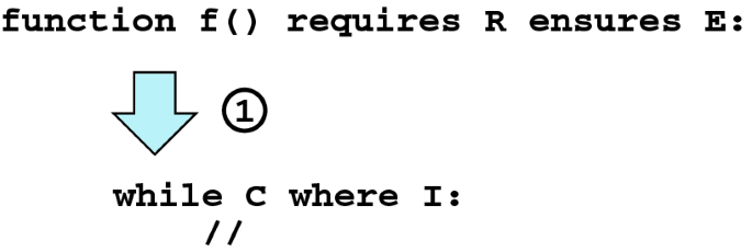
Informally: Information known at the start of loop must imply the loop invariant. Formally, we can express this as:
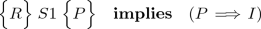
where S1 represents all statements before the loop.
-
2.
Loop Invariants must be maintained.
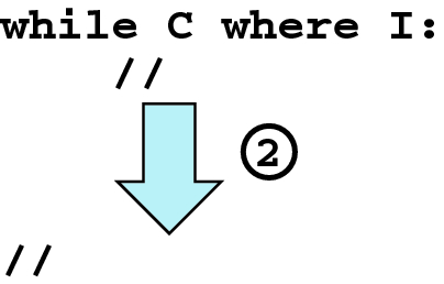
Informally: Assuming only the loop invariant I and the loop condition C hold at the start of the loop body, the information known at the end of the loop body must imply the loop invariant I. Formally:
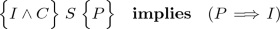
where S represents the loop body.
-
3.
Loop Invariants hold after the loop.
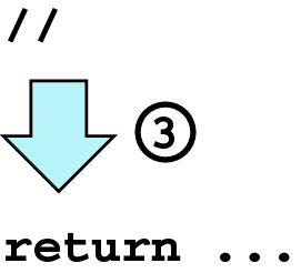
Informally: We can assume that the loop invariant and the negated condition hold after the loop terminates. From just those two assumptions, we must be able to prove that the code after the loop is correct. Formally:
$$ \Big \{I\wedge \!\lnot C\Big \}\;S2\;\Big \{E\Big \} $$where S2 represents all statements after the loop; and E is the postcondition.


The following function, which just counts up to 10, illustrates a very simple loop invariant that captures some information about the range of the loop variable
 .
.

To help relate the Whiley code to the Hoare triples that we are discussing, we show various intermediate assertions that would appear in the Hoare triples for this program. Such intermediate assertions are not normally written in a Whiley program (because the Whiley verifier calculates them automatically), so we show them here as Whiley comments. This provides an outline of a Hoare-style verification that this function meets its specification. Note that this does not prove the function terminates (although we can see that it does) and, in general, this is not our concern here.
Here is another example of a simple loop that sums two arrays pair-wise into an output array. What would be a suitable loop invariant for the loop in this function?

6.2 Ghost Variables and Loop Invariants
A ghost variable is any variable introduced specifically to aid verification in some way, but is unnecessary to execute the program. In the vector sum example above, variable
 is a ghost variable, because we can implement the solution without it, but we cannot verify the solution without it! Here is the loop invariant for the vector sum example, showing how we need to use
 in the loop invariant to refer to the original contents of the
 vector:

Recall that Rule 3 for loops says that the only thing known after a loop is the loop invariant and the negated loop guard. In theory, this means that our loop invariant should include all known facts about all the variables in the function. So perhaps we should add predicates like
 into the loop invariant above, even though neither of these variables are changing within the loop? This would become very verbose and tedious - it is a very common case that some variables are not changed at all within a loop.
Fortunately, Whiley uses an extended form of Rule 3 for variables not modified in a loop: all information about them from before loop is automatically retained. This generally includes all ghost variables (since they typically just capture the previous values of some variable), but also variables like
 in the vector sum example above, because there is no assignment to it in the loop. So for a predicate that does not mention any variables changed by the loop, it is not necessary to include that predicate in the loop invariant, as it will automatically be preserved across the loop.
6.3 Example: Reversing an Array (Implementation)
Now that we have all the necessary tools, such as loop invariants and ghost variables, let us consider what loop invariant is needed to verify the following program, which reverses the contents of an array in-place.

To help visualize the required invariant, imagine that we are half way through reversing the array. The region between i and j remains to be reversed.


6.4 Example: Dutch National Flag
We now consider a more complex example, due to the famous Dutch computer scientist Edsger Dijkstra:
“Given a quantity of items in three colours of the Dutch National flag, partition the items into three groups such that red items come first, then white items and, finally, blue items.”

This can be thought of as a special case of sorting, and is very similar to the “split/partition” part of quicksort. Unlike the real Dutch flag, we don’t know how many of each colour there are, so we can’t use that to predetermine where the three regions should be. Also, we are required to do this in-place, without using additional arrays.
Rather than give the algorithm and then show how to verify it, we will use this problem to illustrate the approach to programming advocated by Dijkstra, in which programs are constructed from their specifications in a way that guarantees their correctness. In particular, loops are designed by first choosing a loop invariant, by weakening the postcondition of the loop, and then designing the loop body so as to maintain the loop invariant while making progress towards termination. This refinement approach to developing programs [48] develops the code step-by-step guided by the specifications, so it typically leads to code that is easier to verify than code just written directly by a programmer without considering the specifications. As functions become larger and more complex, we recommend that a refinement approach should be used, which is why we demonstrate this approach in this final example of this chapter.
In this case, our postcondition is that the array be a permutation of the original, and that it be arranged into three regions containing red, white and blue elements, respectively. Let us introduce two markers,
 and
and
 to mark the ends of these regions—more specifically, to mark the first and elements of the white region. Thus, the final state looks like this (we will explain
 shortly):

We can describe this more formally using Whiley syntax:

The first line specifies the ranges of
 and
and
 . The remaining lines say that each of the three regions contains only values of the appropriate colour. We will omit the permutation condition, since it is easy to verify, and focus on these conditions. The precondition is that the array initially contains only three distinct values:

Our algorithm needs to build these three regions incrementally as it inspects each element of the array. So at an arbitrary point in the process, we will have three regions containing the red, white and blue elements we’ve already seen. We will also have a fourth region containing the elements we haven’t inspected yet.
The algorithm will consist of a loop in which elements are successively taken from the “unseen” region and added to one of the other regions according to its colour. We could keep the “unseen” region to the left of the red region, between the red and white or white and blue regions, or to the right of the blue regions. We will make an arbitrary choice, and keep it between the white and blue regions, and introduce another marker,
 , to mark the start of the “unseen” region, which means that
 is the next element to be put into the correct region.

Again, we can describe this situation formally using Whiley notation:

Again, the first line defines the ranges of the marker variables, and the remaining lines say that the red, white and blue regions only contain values of the appropriate colour. This condition now gives our loop invariant. We can now design the loop around this invariant. Initially, no elements have been inspected, so the red, white and blue regions are empty, and the “unseen” region is the whole array.

So, our initialisation must establish the condition:

This is the precondition for the loop, and we can easily verify that it implies the loop invariant.

The algorithm will terminate when the “unseen” region is empty, i.e. when
 is greater that
 (as shown in the first diagram), so the loop guard is \(mid \le hi\).
We can easily check that the postcondition will hold when the loop invariant is true and the loop guard is false:

Notice that we have already proved two of the correctness conditions for the loop, and we haven’t even written the loop body yet! Now let us consider the loop body. The loop body has to reduce the size of the “unseen” region—this guarantees that we make progress towards termination. We will take the easy approach of reducing by one. Thus, we need to reduce
 , which may happen either by increasing
 or by decreasing
 .
.
The key part of the algorithm is now to determine how we can take the next element from the “unseen” part of the array and add it to one of the other three regions, according to its colour. We want to write something like:

Adding
 to the white region is simple: is it already in the next available place for white, so we just need to increment
 . Adding
 to the blue region is also quite easy. We need to put it just to the left of the existing blue region, in the last location of the “unseen” region. But what do we do with the element that is there? We need to swap with the element at
 , since that location is about to be “vacated”. So in this case we make progress by decreasing
 .
.
The last case is to add
 to the red region. This is a bit harder, because (in general), the space to the right of
 is already part of the white region. But if we swap
 with that element, this will add
 to the red region, and effectively move the white region one place to the right, so we can increment both
 and
and
 .
.

And we are done, the final algorithm is given in Fig. 3. Note: on the Whiley Labs website there is a time limit of 10 s for the whole verification. This program may take a little longer than that to verify, so you might need to verify this program on your own computer with a longer timeout.

Algorithm for solving the Dutch National Flag problem

7 Related Work
We discuss several related tools which provide similar functionality and operation to Whiley. In addition, we examine some of the techniques that underpin these tools.
7.1 Tools
ESC/Java & JML. The Extended Static Checker for Java (ESC/Java) is one of the most influential tools in the area of verifying compilers [28]. The ECS/Java tool was based on earlier work that developed the ESC/Modula-3 tool [23]. The tool provides a verifying compiler for Java programs whose specifications are given as annotations in a subset of JML [12, 41]. The following illustrates a simple method in JML which ESC/Java verifies as correct:

Here, we can see preconditions and postconditions are given for the method, along with an appropriate loop invariant. Recalling our discussion from Sect. 6.2,
 refers to
 on entry to the loop and, hence, we have
 holds in this case.
The ESC/Java tool makes some unsound assumptions when verifying programs. In particular, arithmetic overflow is ignored and loops are treated unsoundly by simply unrolling them for a fixed number of iterations. The tool also provides limited support for reasoning about dynamic memory through the use of ownership annotations and
 clauses for expressing frame conditions. ESC/Java has been demonstrated in some real-world settings. For example, Cataño and Huisman used it to check specifications given for an independently developed implementation of an electronic purse [11]. Unfortunately the development of JML and its associated tooling has stagnated over the last decade, although has more recently picked up again through the OpenJML initiative [17, 18, 54].
Spec#. This system followed ESC/Java and benefited from many of the insights gained in that project. Spec# added proper support for handling loop invariants [6], for handling safe object initialisation [26] and allowing temporary violations of object invariants through the
 keyword [45]. The latter is necessary to address the so-called packing problem which was essentially ignored by ESC/Java [7]. Another departure from ESC/Java was the use of the BOOGIE intermediate language for verification (as opposed to guarded commands) [5], and the Z3 automated theorem prover (as opposed to Simplify) [49]. Both of these mean that Spec# is capable of verifying a wider range of programs than ESC/Java.
Although the Spec# project has now finished, the authors did provide some invaluable reflections on their experiences with the project [6]. Amongst many other things, they commented that:
“Of the unsound features in ESC/Java, many were known to have solutions. But two open areas were how to verify object invariants in the presence of subclassing and dynamically dispatched methods (...) as well as method framing.”
A particular concern was the issue of method re-entrancy, which is particularly challenging to model correctly. Another interesting insight given was that:
“If we were to do the Spec# research project again, it is not clear that extending an existing language would be the best strategy.”
The primary reason for this was the presence of constructs that are difficult for a verifier to reason about, and also the challenge for a small research group in maintaining compatibility with a large and evolving language.
Finally, the Spec# project lives on in various guises. For example, VCC verifies concurrent C code and was developed by reusing much of the tool chain from Spec# [16]. VCC has been successfully used to verify Microsoft’s Hyper-V hypervisor. Likewise, Microsoft recently introduced a Code Contracts library in .NET 4.0 which was inspired by the Spec# project (though mostly focuses on runtime checking).
Dafny. This is perhaps the most comparable related work to Whiley, and was developed independently at roughly the same time [43, 44]. That said, the goals of the Dafny project are somewhat different. In particular, the primary goal of Dafny to provide a proof-assistant for verifying algorithms rather than, for example, generating efficient executable code. In contrast, Whiley aims to generate code suitable for embedded systems [50, 56, 57]. Dafny is an imperative language with simple support for objects and classes without inheritance. Like Whiley, Dafny employs unbound arithmetic and distinguishes between pure and impure functions. Dafny provides algebraic data types (which are similar to Whiley’s recursive data types) and supports immutable collection types with value semantics that are primarily used for ghost fields to enable specification of pointer-based programs. Dynamic memory allocation is possible in Dafny, but no explicit deallocation mechanism is given and presumably any implementation would require a garbage collector.
Unlike Whiley, Dafny also supports generic types and dynamic frames [38]. The latter provides a suitable mechanism for reasoning about pointer-based programs. For example, Dafny has been used successfully to verify the Schorr-Waite algorithm for marking reachable nodes in an object graph [44]. Finally, Dafny has been used to successfully verify benchmarks from the VSTTE’08 [46], VSCOMP’10 [39], VerifyThis’12 [36] challenges (and more).
7.2 Techniques
Hoare provided the foundation for formalising work in this area with his seminal paper introducing Hoare Logic [34]. This provides a framework for proving that a sequence of statements meets its postcondition given its precondition. Unfortunately Hoare logic does not tell us how to construct such a proof; rather, it gives a mechanism for checking a proof is correct. Therefore, to actually verify a program is correct, we need to construct proofs which satisfy the rules of Hoare logic.
The most common way to automate the process of verifying a program is with a verification condition generator. As discussed in Sect. 5.4, such algorithms propagate information in either a forwards or backwards direction. However, the rules of Hoare logic lend themselves more naturally to the latter [31]. Perhaps for this reason, many tools choose to use the weakest precondition transformer. For example, ESC/Java computes weakest preconditions [28], as does the Why platform [27], Spec# [8], LOOP [37], JACK [9] and SnuggleBug [13]. This is surprising given that it leads to fewer verification conditions and, hence, makes it harder to generate useful error messages (recall our discussion from Sect. 5.4). To workaround this, Burdy et al. embed path information in verification conditions to improve error reporting [9]. A similar approach is taken in ESC/Java, but requires support from the underlying automated theorem prover [22]. Denney and Fischer extend Hoare logic to formalise the embedding of information within verification conditions [21]. Again, their objective is to provide useful error messages.
A common technique for generating verification conditions is to transform the input program into passive form [8, 23, 28, 33]. Here, the control-flow graph of each function is converted using standard techniques into a reducible (albeit potentially larger) graph. This is then further reduced by eliminating loops to leave an acyclic graph, before a final transformation into Static Single Assignment form (SSA) [19, 20]. The main advantage is that, after this transformation, generating verification conditions becomes straightforward. Furthermore, the technique works well for unstructured control flow and can be tweaked to produced compact verification conditions [2, 3, 29, 42].
Dijkstra’s Guarded Command Language provides an alternative approach to the generation of verification conditions [24]. In this case, the language is far removed from the simple imperative language of Hoare logic and, for example, contains only the sequence and non-deterministic choice constructs for handling control-flow. There is rich history of using guarded commands as an intermediate language for verification, which began with the ECS/Modula-3 tool [23]. This was continued in ESC/Java and, during the later development of Spec#, a richer version (called Boogie) was developed [5]. Such tools use guarded commands as a way to represent programs that are in passive form (discussed above) in a human-readable manner. As these programs are acyclic, the looping constructs of Dykstra’s original language are typically ignored.
Finally, it is worth noting that Frade and Pinto provide an excellent survey of verification condition generation for simple While programs [31]. They primarily focus on Hoare Logic and various extensions, but also explore Dijkstra’s Guarded Command Language. They consider an extended version of Hoare’s While Language which includes user-provided loop invariants. They also present an algorithm for generating verification conditions based on the weakest precondition transformer.
8 Conclusions
In this chapter we have introduced the basic ideas of verifying simple imperative code. With just the executable code, a verifying compiler does not know what the program is intended to do, so all it can verify is that the code will execute without errors such as: array indexes out of bounds, division by zero.
But if we add some specification information, such as preconditions to express the input assumptions and postconditions to express the desired results, then the verifying compiler can check much richer properties. If the postconditions are strong enough to express the complete desired behavior of the function, then the verifying compiler can even check full functional correctness.
In practice, the reasoning abilities of verifying compilers are gradually improving with time, and at the current point in time it is usually necessary to annotate our programs with extra information to aid verification, such as loop invariants and data invariants. One can argue that it is good engineering practice to document these properties for other human readers anyway, even if the verifying compiler did not need them. But in the future, we envisage that verification tools will become smarter about inferring obvious invariants, which will gradually reduce the burden on human verifiers.
Notes
- 1.
This holds because integers are unbounded in Whiley.
References
European Space Agency: Ariane 5: Flight 501 failure. Report by the Enquiry Board (1996)
Babić, D., Hu, A.J.: Exploiting shared structure in software verification conditions. In: Yorav, K. (ed.) HVC 2007. LNCS, vol. 4899, pp. 169–184. Springer, Heidelberg (2008). https://doi.org/10.1007/978-3-540-77966-7_15
Babić, D., Hu, A.J.: Structural abstraction of software verification conditions. In: Damm, W., Hermanns, H. (eds.) CAV 2007. LNCS, vol. 4590, pp. 366–378. Springer, Heidelberg (2007). https://doi.org/10.1007/978-3-540-73368-3_41
Back, R.J.R., von Wright, J.: Refinement Calculus: A Systematic Approach. Graduate Texts in Computer Science. Springer, New York (1998). https://doi.org/10.1007/978-1-4612-1674-2
Barnett, M., Chang, B.-Y.E., DeLine, R., Jacobs, B., Leino, K.R.M.: Boogie: a modular reusable verifier for object-oriented programs. In: de Boer, F.S., Bonsangue, M.M., Graf, S., de Roever, W.-P. (eds.) FMCO 2005. LNCS, vol. 4111, pp. 364–387. Springer, Heidelberg (2006). https://doi.org/10.1007/11804192_17
Barnett, M., Fähndrich, M., Leino, K.R.M., Müller, P., Schulte, W., Venter, H.: Specification and verification: the Spec# experience. Commun. ACM 54(6), 81–91 (2011)
Barnett, M., DeLine, R., Fähndrich, M., Leino, K.R.M., Schulte, W.: Verification of object-oriented programs with invariants. J. Object Technol. 3(6), 27–56 (2004)
Barnett, M., Leino, K.R.M.: Weakest-precondition of unstructured programs. In: Proceedings of the Workshop on Program Analysis for Software Tools and Engineering (PASTE), pp. 82–87. ACM Press (2005)
Burdy, L., Requet, A., Lanet, J.-L.: Java applet correctness: a developer-oriented approach. In: Araki, K., Gnesi, S., Mandrioli, D. (eds.) FME 2003. LNCS, vol. 2805, pp. 422–439. Springer, Heidelberg (2003). https://doi.org/10.1007/978-3-540-45236-2_24
Carvalho, M., DeMott, J., Ford, R., Wheeler, D.: Heartbleed 101. IEEE Secur. Priv. 12(4), 63–67 (2014)
Cataño, N., Huisman, M.: Formal specification and static checking of gemplus’ electronic purse using ESC/Java. In: Eriksson, L.-H., Lindsay, P.A. (eds.) FME 2002. LNCS, vol. 2391, pp. 272–289. Springer, Heidelberg (2002). https://doi.org/10.1007/3-540-45614-7_16
Chalin, P., Rioux, F.: JML runtime assertion checking: improved error reporting and efficiency using strong validity. In: Cuellar, J., Maibaum, T., Sere, K. (eds.) FM 2008. LNCS, vol. 5014, pp. 246–261. Springer, Heidelberg (2008). https://doi.org/10.1007/978-3-540-68237-0_18
Chandra, S., Fink, S.J., Sridharan, M.: Snugglebug: a powerful approach to weakest preconditions. In: Proceedings of the ACM conference on Programming Language Design and Implementation (PLDI), pp. 363–374. ACM Press (2009)
Charette, R.: This car runs on code. IEEE Spectr. 46, 3 (2009)
Charette, R.N.: Why software fails. IEEE Spect. 42(9), 42–49 (2005)
Cohen, E., et al.: VCC: a practical system for verifying concurrent C. In: Berghofer, S., Nipkow, T., Urban, C., Wenzel, M. (eds.) TPHOLs 2009. LNCS, vol. 5674, pp. 23–42. Springer, Heidelberg (2009). https://doi.org/10.1007/978-3-642-03359-9_2
Cok, D.R.: OpenJML: JML for Java 7 by extending OpenJDK. In: Bobaru, M., Havelund, K., Holzmann, G.J., Joshi, R. (eds.) NFM 2011. LNCS, vol. 6617, pp. 472–479. Springer, Heidelberg (2011). https://doi.org/10.1007/978-3-642-20398-5_35
Cok, D.R.: OpenJML: Software verification for Java 7 using JML, OpenJDK, and eclipse. In: Proceedings of the Workshop on Formal Integrated Development Environment (F-IDE), vol. 149, pp. 79–92 (2014)
Cytron, R., Ferrante, J., Rosen, B., Wegman, M., Zadeck, F.K.: An efficient method of computing static single assignment form. In: Proceedings of the ACM symposium on the Principles Of Programming Languages (POPL), pp. 25–35 (1989)
Cytron, R., Ferrante, J., Rosen, B.K., Wegman, M.N., Zadeck, F.K.: Efficiently computing static single assignment form and the control dependence graph. ACM Trans. Program. Lang. Syst. 13(4), 451–490 (1991)
Denney, E., Fischer, B.: Explaining verification conditions. In: Meseguer, J., Roşu, G. (eds.) AMAST 2008. LNCS, vol. 5140, pp. 145–159. Springer, Heidelberg (2008). https://doi.org/10.1007/978-3-540-79980-1_12
Detlefs, D., Nelson, G., Saxe, J.B.: Simplify: a theorem prover for program checking. J. ACM 52(3), 365–473 (2005)
Detlefs, D.L., Leino, K.R.M., Nelson, G., Saxe, J.B.: Extended static checking. SRC Research Report 159, Compaq Systems Research Center (1998)
Dijkstra, E.W.: Guarded commands, nondeterminancy and formal derivation of programs. Commun. ACM 18, 453–457 (1975)
Durumeric, Z., et al.: The matter of heartbleed. In: Proceedings of Internet Measurement Conference (IMC), pp. 475–488. ACM Press (2014)
Fähndrich, M., Leino, K.R.M.: Declaring and checking non-null types in an object-oriented language. In: Proceedings of the ACM conference on Object-Oriented Programming, Systems, Languages and Applications (OOPSLA), pp. 302–312. ACM Press (2003)
Filliâtre, J.-C., Marché, C.: The Why/Krakatoa/Caduceus platform for deductive program verification. In: Damm, W., Hermanns, H. (eds.) CAV 2007. LNCS, vol. 4590, pp. 173–177. Springer, Heidelberg (2007). https://doi.org/10.1007/978-3-540-73368-3_21
Flanagan, C., Leino, K., Lillibridge, M., Nelson, G., Saxe, J.B., Stata, R.: Extended static checking for Java. In: Proceedings of the ACM conference on Programming Language Design and Implementation (PLDI), pp. 234–245 (2002)
Flanagan, C., Saxe, J.B.: Avoiding exponential explosion: generating compact verification conditions. In: Proceedings of the ACM symposium on the Principles Of Programming Languages (POPL), pp. 193–205. ACM Press (2001)
Floyd, R.W.: Assigning meaning to programs. In: Proceedings of Symposia in Applied Mathematics, vol. 19, pp. 19–31. American Mathematical Society (1967)
Frade, M.J., Pinto, J.S.: Verification conditions for source-level imperative programs. Comput. Sci. Rev. 5(3), 252–277 (2011)
Software problem led to system failure at dhahran, saudi arabia, gao report #b-247094 (1992)
Grigore, R., Charles, J., Fairmichael, F., Kiniry, J.: Strongest postcondition of unstructured programs. In: Proceedings of the Workshop on Formal Techniques for Java-like Programs (FTFJP), pp. 6:1–6:7. ACM Press (2009)
Hoare, C.A.R.: An axiomatic basis for computer programming. CACM 12, 576–580 (1969)
Holzmann, G.J.: Out of bounds. IEEE Softw. 32(6), 24–26 (2015)
Huisman, M., Klebanov, V., Monahan, R.: Verifythis verification competition 2012 - organizer’s report (2013)
Jacobs, B.: Weakest pre-condition reasoning for Java programs with JML annotations. J. Log. Algebr. Program. 58(1–2), 61–88 (2004)
Kassios, I.T.: Dynamic frames: support for framing, dependencies and sharing without restrictions. In: Misra, J., Nipkow, T., Sekerinski, E. (eds.) FM 2006. LNCS, vol. 4085, pp. 268–283. Springer, Heidelberg (2006). https://doi.org/10.1007/11813040_19
Klebanov, V., et al.: The 1st verified software competition: experience report. In: Butler, M., Schulte, W. (eds.) FM 2011. LNCS, vol. 6664, pp. 154–168. Springer, Heidelberg (2011). https://doi.org/10.1007/978-3-642-21437-0_14
Ko, A.J., Dosono, B., Duriseti, N.: Thirty years of software problems in the news. In: Proceedings of the 7th International Workshop on Cooperative and Human Aspects of Software Engineering, CHASE 2014, Hyderabad, India, 2–3 June 2014. ACM Press (2014)
Leavens, G.T., Cheon, Y., Clifton, C., Ruby, C., Cok, D.R.: How the design of JML accommodates both runtime assertion checking and formal verification. Sci. Comput. Program. 55(1–3), 185–208 (2005)
Leino, K.R.M.: Efficient weakest preconditions. Inf. Process. Lett. 93(6), 281–288 (2005)
Rustan, K., Leino, M.: Developing verified programs with Dafny. In: Joshi, R., Müller, P., Podelski, A. (eds.) VSTTE 2012. LNCS, vol. 7152, p. 82. Springer, Heidelberg (2012). https://doi.org/10.1007/978-3-642-27705-4_7
Leino, K.R.M.: Dafny: an automatic program verifier for functional correctness. In: Clarke, E.M., Voronkov, A. (eds.) LPAR 2010. LNCS (LNAI), vol. 6355, pp. 348–370. Springer, Heidelberg (2010). https://doi.org/10.1007/978-3-642-17511-4_20
Leino, K.R.M., Müller, P.: Using the Spec# language, methodology, and tools to write bug-free programs. In: Müller, P. (ed.) LASER 2007–2008. LNCS, vol. 6029, pp. 91–139. Springer, Heidelberg (2010). https://doi.org/10.1007/978-3-642-13010-6_4
Leino, K.R.M., Monahan, R.: Dafny meets the verification benchmarks challenge. In: Leavens, G.T., O’Hearn, P., Rajamani, S.K. (eds.) VSTTE 2010. LNCS, vol. 6217, pp. 112–126. Springer, Heidelberg (2010). https://doi.org/10.1007/978-3-642-15057-9_8
Leveson, N., Turner, C.: An investigation of the Therac-25 accidents. IEEE Comput. 26(7), 18–41 (1993)
Morgan, C.: Programming from Specifications, 2nd edn. Prentice Hall, Upper Saddle River (1994)
de Moura, L., Bjørner, N.: Z3: an efficient SMT solver. In: Ramakrishnan, C.R., Rehof, J. (eds.) TACAS 2008. LNCS, vol. 4963, pp. 337–340. Springer, Heidelberg (2008). https://doi.org/10.1007/978-3-540-78800-3_24
Pearce, D.J.: Integer range analysis for Whiley on embedded systems. In: Proceedings of the IEEE/IFIP Workshop on Software Technologies for Future Embedded and Ubiquitous Systems, pp. 26–33 (2015)
Pearce, D.J.: The Whiley Language Specification (Updated, 2016)
Pearce, D.J., Groves, L.: Whiley: a platform for research in software verification. In: Erwig, M., Paige, R.F., Van Wyk, E. (eds.) SLE 2013. LNCS, vol. 8225, pp. 238–248. Springer, Cham (2013). https://doi.org/10.1007/978-3-319-02654-1_13
Rahman, H.A., Beznosov, K., Martí, J.R.: Identification of sources of failures and their propagation in critical infrastructures from 12 years of public failure reports. Int. J. Crit. Infrastruct. 5(3), 220–244 (2009)
Sánchez, J., Leavens, G.T.: Static verification of PtolemyRely programs using OpenJML. In: Proceedings of the Workshop on Foundations of Aspect-Oriented Languages (FOAL), pp. 13–18. ACM Press (2014)
Steinberg, J.: Massive internet security vulnerability - here’s what you need to do (2014). https://www.forbes.com/sites/josephsteinberg/2014/04/10/massive-internet-security-vulnerability-you-are-at-risk-what-you-need-to-do. Accessed 12 Jan 2019
Stevens, M.: Demonstrating Whiley on an embedded system. Technical report, School of Engineering and Computer Science, Victoria University of Wellington (2014). http://www.ecs.vuw.ac.nz/~djp/files/MattStevensENGR489.pdf
Weng, M.H., Pfahringer, B., Utting, M.: Static techniques for reducing memory usage in the C implementation of Whiley programs. In: Proceedings of the Australasian Computer Science Week Multiconference, ACSW 2017, pp. 15:1–15:8. ACM, New York (2017). https://doi.org/10.1145/3014812.3014827
White, D., Roschelle, A., Peterson, P., Schlissel, D., Biewald, B., Steinhurst, W.: The 2003 blackout: solutions that won’t cost a fortune. Electr. J. 16(9), 43–53 (2003)
Acknowledgements
Thanks to all the students and researchers who have contributed to the development of Whiley. The slides used to present this tutorial at SETSS were based on David Pearce’s slides for the SWEN224 (Software Correctness) course at Victoria University of Wellington, 2015-2016. Thanks to the students of those classes for their feedback and comments. Thanks to Professor Zhiming LIU for organising SETSS 2018.
Author information
Authors and Affiliations
Corresponding author
Editor information
Editors and Affiliations
Appendix A: Sample Answers to Selected Exercises
Appendix A: Sample Answers to Selected Exercises
This appendix gives sample solutions to the exercises that cannot be checked using the online Whiley Labs website.


Rights and permissions
Copyright information
© 2019 Springer Nature Switzerland AG
About this chapter

Cite this chapter
Pearce, D.J., Utting, M., Groves, L. (2019). An Introduction to Software Verification with Whiley. In: Bowen, J., Liu, Z., Zhang, Z. (eds) Engineering Trustworthy Software Systems. SETSS 2018. Lecture Notes in Computer Science(), vol 11430. Springer, Cham. https://doi.org/10.1007/978-3-030-17601-3_1
Download citation
DOI: https://doi.org/10.1007/978-3-030-17601-3_1
Published:
Publisher Name: Springer, Cham
Print ISBN: 978-3-030-17600-6
Online ISBN: 978-3-030-17601-3
eBook Packages: Computer ScienceComputer Science (R0)