Relativistic Atomic Structure

Abstract

Relativistic quantum mechanics is required for the description of atoms and molecules whenever their orbital electrons probe regions of space with high potential energy near the atomic nuclei. Primary effects of a relativistic description include changes to spatial and momentum distributions; spin-orbit interactions; quantum electrodynamic corrections such as the Lamb shift; and vacuum polarization. Secondary effects in many-electron systems arise from shielding of the outer electrons by the distributions of electrons in penetrating orbitals; they change orbital binding energies and dimensions and so modify the order in which atomic shells are filled in the lower rows of the Periodic Table.

Relativistic atomic and molecular structure theory can be regarded as a simplification of the fundamental description provided by quantum electrodynamics (QED). This treats the atom or molecule as an assembly of electrons and atomic nuclei interacting primarily by exchanging photons. This model is far too difficult and general for most purposes, and simplifications are required. The most important of these is the representation of the nuclei as classical charge distributions, or even as point particles. Since the motion of the nuclei is usually slow relative to the electrons, it is often adequate to treat the nuclear motion nonrelativistically, or even to start from nuclei in fixed positions, correcting subsequently for nuclear motion.

The emphasis in this chapter is on relativistic methods for the calculation of atomic structure for general many-electron atoms based on an effective Hamiltonian derived from QED in the manner sketched in Sect. 22.2 below. An understanding of the Dirac equation, its solutions and their numerical approximation, is essential material for studying many-electron systems, just as the corresponding properties of the Schrödinger equation underpin Chapt. 21. We shall use atomic units throughout. Where it aids interpretation we shall, however, insert factors of c, m _e and ℏ. In these units, the velocity of light, c, has the numerical value α ⁻¹ =137.03599911 (46), where α is the fine structure constant.

These keywords were added by machine and not by the authors. This process is experimental and the keywords may be updated as the learning algorithm improves.

Mathematical Preliminaries

Relativistic Notation: Minkowski Space-Time

An event in Minkowski space-time is defined by a 4-vector x ={ x ^μ} (μ = 0, 1, 2, 3) where x ⁰ = ct is the time coordinate and x ¹, x ², x ³ are Cartesian coordinates in 3-space. The bilinear form (The Einstein suffix convention, in which repeated pairs of Greek subscripts are assumed to be summed over all values 0, 1, 2, 3, will be used where necessary in this chapter.)

(22.1)

in which

(22.2)

are called metric coefficients, defines the metric of Minkowski space.

Lorentz Transformations

Lorentz transformations are defined as linear mappings Λ such that

(22.3)

so that

(22.4)

This furnishes 10 equations connecting the 16 components of Λ; at most 6 components can be regarded as independent parameters. The (infinite) set of Λ matrices forms a regular matrix group (with respect to matrix multiplication) called the Lorentz group, , designated O(3,1) [22.1,2].

Classification of Lorentz Transformations

Rotations

Lorentz transformations with matrices of the form

(22.5)

where R ∈ SO(3) is an orthogonal 3 × 3 matrix with determinant + 1, and 0 is a null three dimensional column vector, correspond to three-dimensional space rotations. They form a group isomorphic to SO(3).

Boosts

Lorentz transformations with matrices of the form

(22.6)

with v = v n a three dimensional column vector, | n | = 1, v = | v | and γ(v) = (1 − v ²/c ²)^−1/2, are called boosts. The matrix Λ describes an ‘active’ transformation from an inertial frame in which a free classical particle is at rest to another inertial frame in which its velocity is v.

Boosts form a submanifold of though they do not in general form a subgroup. However, the set of boosts in a fixed direction n form a one-parameter subgroup.

Discrete Transformations

The matrices

(22.7)

are called discrete Lorentz transformations and form a subgroup of the Lorentz group along with the identity I ₄. The matrix P performs space or parity inversion; the matrix T performs time reversal.

Infinitesimal Lorentz Transformations

The proper Lorentz transformations close to the identity are of particular importance: they have the form

(22.8)

and ϵ is infinitesimal. The infinitesimal generators, components ω _μν , can be treated as quantum mechanical observables: see Sect. 22.2.1.

The Lorentz Group

The Lorentz group is a Lie group with a six-dimensional group manifold which has four connected components, namely

(22.9)

(22.10)

(22.11)

(22.12)

The connected component containing the identity is a Lie subgroup of called the proper Lorentz group. All its group elements can be obtained from boosts and rotations. It is not simply connected because the subgroup of rotations is not simply connected. The group is also noncompact as the subset of boosts is homeomorphic to .

These topological properties of are essential for understanding the properties of relativistic wave equations. In particular the multiple connectedness forces the introduction of spinor representations, and to the appearance of half-integer angular momenta or spin.

Contravariant and Covariant Vectors

Contravariant 4-vectors (such as events x) transform according to the rule

(22.13)

Covariant 4-vectors can be formed by writing

(22.14)

so that

(22.15)

is invariant with respect to Lorentz transformations. Similarly, we can construct a contravariant 4-vector from a covariant one by writing

(22.16)

The transformation law for covariant vectors is therefore

(22.17)

The most important example of a covariant vector is the 4-momentum operator

(22.18)

From this we derive the contravariant 4-momentum operator with components p ^μ by writing

(22.19)

in agreement with nonrelativistic expressions.

Poincaré Transformations

More generally, a Poincaré transformation is obtained by combining Lorentz transformations and space-time translations:

(22.20)

The set of all Poincaré transformations, Π = (a, Λ), with the composition law

(22.21)

also forms a group, .

Properties of the Lorentz and Poincaré groups will be introduced as needed. For a concise account of their properties see [22.3]. For more detail on relativistic quantum mechanics in general see textbooks such as [22.3,4].

Dirac's Equation

We present Dirac's equation for an electron in a classical electromagnetic field defined by the 4-potential A _μ (x):

Covariant Form

(22.22)

where

Here, and elsewhere in this chapter, identity matrices are omitted when it is safe to do so.

Dirac Gamma Matrices

• Anticommutation relations:

  

• Standard representation:

  

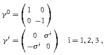
where σ _i (i = 1, 2, 3) are Pauli matrices [22.1,2,3,4].

Noncovariant Form

In the majority of atomic structure calculations, a frame of reference is chosen in which the nuclear center is taken to be fixed at the origin. In this case it is convenient to write Dirac's equation in noncovariant form. Then functions of

where x ⁰ = ct, can be regarded as functions of the time t and the position 3-vector x, so that (22.22) is replaced by

(22.23)

where the scalar and 3-vector potentials are defined by

(22.24)

and

(22.25)

defines the Dirac Hamiltonian. The matrices α, with Cartesian components , and β, have the standard representation

(22.26)

(22.27)

Characterization of Dirac States

The solutions of Dirac's equation span representations of the Lorentz and Poincaré groups, whose infinitesimal generators can be identified with physical observables. The Lorentz group algebra has 10 independent self-adjoint infinitesimal generators: these can be taken to be the components p ^μ of the four-momentum (which generate displacements in each of the four coordinate directions); the three generators, J _i , of rotations about each coordinate axis in space; and the pseudovector w _μ . The irreducible representations can be characterized by invariants

(22.28)

(22.29)

where p is the momentum four-vector and s is a 3-vector defined in terms of Pauli matrices by

which can be interpreted as the electronic angular momentum (intrinsic spin) in its rest frame. For more detail see [22.3] and the original papers [22.5,6].

The Charge-Current 4-Vector

Dirac's equation (22.22) is covariant with respect to Lorentz (22.3) and Poincaré (22.20) transformations, provided that there exists a nonsingular 4 × 4 matrix S(Λ) with the property

(22.30)

The matrices S(Λ) are characterized by the equation

(22.31)

The most important observable expression required in this chapter is the charge-current four-vector

(22.32)

where the Dirac adjoint is defined by

(22.33)

and the dagger denotes spinor conjugation and transposition. Since

j ^μ(x) transforms as a 4-vector

by virtue of (22.31). The component j ⁰(x) can be interpreted as a multiple of the charge density ρ(x),

(22.34)

and the space-like components as the current density

(22.35)

The charge-current density satisfies a continuity equation, which in noncovariant form reads

or, in covariant notation,

(22.36)

This is readily proved by using the Dirac equation (22.22) and its Dirac adjoint. Equation (22.36) is clearly invariant under Poincaré transformations, and this yields the important property that electric charge is conserved in Dirac theory.

QED: Relativistic Atomic and Molecular Structure

The QED Equations of Motion

The conventional starting point [22.7,8,9,10] for deriving equations of motion in quantum electrodynamics (QED) is a Lagrangian density of the form

(22.37)

The first term is the Lagrangian density for the free electromagnetic field, F ^μν(x),

(22.38)

the second term is the Lagrangian density for the electron-positron field in the presence of the external potential A ^μ _ext(x),

(22.39)

We assume that the electromagnetic fields are expressible in terms of the four-potentials by

where

is the sum of a four-potential A ^μ _ext(x) describing the fields generated by classical external charge-current distributions, and a quantized field A ^μ(x) which through

(22.40)

accounts for the interaction between the uncoupled electrons and the radiation field. The field equations deduced from (22.37) are

(22.41)

and clearly exhibit the coupling between the fields.

Quantum electrodynamics requires the solution of the system (22.41) when A ^μ(x), ψ(x) and its adjoint are quantized fields. This formulation is purely formal: it ignores all questions of zero-point energies, normal ordering of operators, choice of gauge associated with the quantized photon field, or the need to include (infinite) counterterms to render the theory finite.

The Quantized Electron-Positron Field

Furry's bound interaction picture of QED [22.7,11] exploits the fact that a one-electron model is often a good starting point for a more accurate calculation of atomic or molecular properties. The electrons are described by a field operator

(22.42)

where E _F ≥− mc ² is a “Fermi level” separating the states describing electrons (bound and continuum) from the positron states (lower continuum) in the chosen time-independent model potential V(r). Equation (22.42) is written as if the spectrum were entirely discrete, as in finite matrix models; more generally, this must be replaced by integrals over the continuum states together with a sum over the bound states. We assume that the amplitudes ψ _m (x) are orthonormalized (which can be achieved, for example, by enclosing the system in a finite box). The operators a _m and a _m ^† respectively annihilate and create electrons, and b _n and b _n ^† perform the same role for vacancies in the “negative energy” states, which we interpret as antiparticles (positrons). These operators satisfy the anticommutation rules (see Sect. 6.1.1)

(22.43)

where [a, b] = ab + ba. All other anticommutators vanish. The operator representing the number of electrons in state m is then

(22.44)

having the eigenvalues 0 or 1; the states of a system of noninteracting electrons and positrons can therefore be labeled by listing the occupation numbers, 0 or 1 of the one-electron states participating.

We define the vacuum state as the (reference) state |0〉 in which N _m  = N _n  = 0 for all m, n, so that

(22.45)

The operator representing the total number of particles is given by

This is not quite satisfactory: is infinite for the vacuum state, as are the total charge and energy of the vacuum.

These infinite “zero-point” values can be eliminated by introducing normal ordered operators. A product of annihilation and creation operators is in normal order if it is rearranged so that all annihilation operators are to the right of all creation operators. Such a product has a null value in the vacuum state. In performing the rearrangement, each anticommutator is treated as if it were zero. We denote normal ordering by placing the operators between colons. Thus : a _m ^† a _m :  =  a _m ^† a _m whilst :b _n b ^† _n :  =− b ^† _n b _n . This means that if we redefine N by

(22.46)

then 〈0|N|0〉 = 0. The same trick eliminates the infinity from the total energy of the vacuum;

(22.47)

so that 〈0|H ₀ |0〉 = 0.

The current density operator is given by the commutator of two field variables

(22.48)

where the Dirac adjoint, is defined by (22.33). The definition (22.48) differs from (22.32) by expressing the total current as the difference between the electron (negatively charged) and positron (positively charged) currents. We can write

(22.49)

where S _F(x, y) is the Feynman causal propagator , defined below. Since 〈0|:j ^μ(x):|0〉 = 0, the last term in (22.49) is the vacuum polarization current due to the asymmetry between positive and negative energy states induced by the external field. From this, the net charge of the system is

(22.50)

Q _vac is the total charge of the vacuum, which vanishes for free electrons, but is finite in the presence of an external field (the phenomenon of vacuum polarization). Note that whilst Q is conserved for all processes, the total number of particles need not be; it is always possible to add virtual states incorporating electron-positron pairs without changing Q.

Quantized Electromagnetic Field

The four-potential of the quantized electromagnetic field can be expressed in terms of a spectral expansion over the field modes in, for example, plane waves

(22.51)

The vectors ϵ _μ ^(λ)(k) describe the polarization modes; there are four linearly independent vectors, which may be assumed real, for each k on the positive light cone. Two of these (λ = 1, 2) can be chosen perpendicular to the photon momentum k (transverse polarization); one component (λ = 3) along k (longitudinal polarization); and the final component (λ = 0) is time-like (scalar polarization). The operators q ^(λ)(k) and q ^(λ)†(k) describe respectively photon absorption and emission. They satisfy commutation relations

(22.52)

all other commutators vanish. The photon vacuum state, |0〉 _γ , is such that

(22.53)

Further details may be found in the texts [22.7,8,9,10].

QED Perturbation Theory

The textbook perturbation theory of QED, see for example [22.7,8,10,12] and other works, has been adapted for applications to relativistic atomic and molecular structure and is also the source of methods of nonrelativistic many-body perturbation theory (MBPT). We offer a brief sketch emphasizing details not found in the standard texts.

The Perturbation Expansion

The Lagrangian approach leads to an interaction Hamiltonian

(22.54)

In the interaction representation, this gives an equation of motion

(22.55)

where |Φ(t)〉 is the QED state vector, and

where H ₀ = H _em + H _e is the Hamiltonian for the uncoupled photon and electron-positron fields. If S(t, t′) is the time development operator such that

then

The equivalent integral equation, incorporating the inital condition S(t, t) = 1,

(22.56)

can be solved iteratively, giving

(22.57)

where

This can be put into a more symmetric form by using time-ordered operators. Define the T-product of two operators by

(22.58)

where the positive sign refers to the product of photon operators and the negative sign to electrons. Then

(22.59)

The operator S(t, t′) relates the state vector at time t to the state vector at some earlier time t′ < t. Its matrix elements therefore give the transition amplitudes for different processes, for example the emission or absorption of radiation by a system, or the outcome of scattering of a projectile from a target. The techniques for extracting cross-sections and other observable quantities from the S-operator are described at length in the texts [22.7,8,10,12].

Although the use of normal ordering means that the charge and mass of the reference state, the vacuum, is zero, it fails to remove other infinities due to the occurrence of divergent integrals. The method of extracting finite quantities from this theory involves renormalization of the charge and mass of the electron. We shall refer especially to [22.10, Chapt. 8] for a detailed discussion. The most difficult technical problems are posed by mass renormalization. Formally, we modify the interaction Hamiltonian to read

where δM(x) is the mass renormalization operator

where δm is infinite.

A further problem is that electrons in a many-electron atom or molecule move in a potential which is quite unlike that of the bare nucleus. It is therefore useful to introduce a local mean field potential, say U(x), representing some sort of average interaction with the rest of the electron charge distribution, so that the zero-order orbitals satisfy

(22.60)

With this starting point, the interaction Hamiltonian becomes

(22.61)

where

and the electron current is defined in terms of the mean field orbitals of (22.60). The expression H _I ⁽²⁾(x) is sometimes referred to as a fluctuation potential. The term j ^μ(x)A _μ (x) is proportional to the electron charge, e, which serves as an ordering parameter for perturbation expansions.

Effective Interactions

Although the S-matrix formalism provides in principle a complete computational scheme for many-electron systems, it is generally too cumbersome for practical use, and approximations are necessary. Usually, this is a matter of selecting a subset of dominant contributions to the perturbation series depending on the application. We are faced with the evaluation of T-products of the form

which is done using Wick's Theorem [22.10, p. 25].

In the simplest case,

(22.62)

The vacuum expectation value is called a contraction. More generally, we have

This result has the effect that a T-product with an odd number of factors vanishes. A rigorous statement can be found in all standard texts; each term in the expansion gives rise to a Feynman diagram which can be interpreted as the amplitude of a physical process. As an example, consider the simple but important case

(22.63)

One of the terms (there are others) found by using Wick's Theorem is

We see that this involves the contraction of two photon amplitudes

which plays the role of a propagator (22.69): it relates the photon amplitudes at two space-time points x, y. With the introduction of a spectral expansion for the electron current (22.48), the contribution to the energy of the system becomes

(22.64)

which can be interpreted, in the familiar language of ordinary quantum mechanics, as the energy of two electrons due to the electron-electron interaction V which is directly related to the photon propagator.

Propagators

Propagators relate field variables at different space-time points. Here we briefly define those most often needed in atomic and molecular physics.

Electrons

Define Feynman's causal propagator for the electron-positron field by the contraction

(22.65)

This has a spectral decomposition of the form

(22.66)

which ensures that positive energy solutions are propagated forwards in time, and negative energy solutions backwards in time in accordance with the antiparticle interpretation of the negative energy states. By noting that the stationary state solutions ψ _m (x) have time dependence exp (− iE _m t), we can write (22.66) in the form

(22.67)

where δ is a small positive number, the sum over n includes the whole spectrum, and where the Green's function G(x ₂, x ₁, z), in the specific case in which the potential of the external field a ^μ(x) has only a scalar time-independent part, V _nuc(x), satisfies

(22.68)

G(x ₂, x ₁, z) is a meromorphic function of the complex variable z with branch points at z =± c ², and cuts along the real axis and . The poles lie on the segment at the bound eigenvalues of the Dirac Hamiltonian for this potential.

Photons

The photon propagator D _Fμν (x ₂ − x ₁) is constructed in a similar manner:

(22.69)

where μ ₀ is the permeability of the vacuum. This has the integral representation

(22.70)

where

and δ is a small positive number. This is not unique, as the four-potentials depend on the choice of gauge; for details see [22.8, Sect. 77]. The various forms for the electron-electron interaction given below express such gauge choices.

Effective Interaction of Electrons

The expression (22.63) can be viewed in several ways: it is the interaction of the current density j ^μ(x) at the space-time point x with the four-potential due to the current j ^μ(y); the interaction of the current density j ^μ(y) with the four-potential due to the current j ^μ(x); or, as is commonly assumed in nonrelativistic atomic theory, the effective interaction between two charge density distributions, as represented by (22.64). In terms of the corresponding Feynman diagram, it can be thought of as the energy due to the exchange of a virtual photon.

The form of V depends on the choice of gauge potential, as follows.

Feynman Gauge

(22.71)

where

(22.72)

with

This interaction gives both a real and an imaginary contribution to the energy; only the former is usually taken into account in structure calculations. Since the orbital indices are dummy variables, it is usual to symmetrize the interaction kernel by writing

which places the orbitals on an equal footing.

Coulomb Gauge

Here the Feynman propagator is replaced by that for the Coulomb gauge, giving

(22.73)

in which the operator ∇ involves differentiation with respect to R.

Symmetrization is also used with this interaction.

Breit Operator

The low frequency limit, ω _rp  → 0,  ω _sq  → 0, is known as the Breit interaction:

(22.74)

where

Gaunt Operator

This is a further approximation in which v ^B(R) is replaced by

(22.75)

the residual part of the Breit interaction being neglected.

Comments

The choice of gauge should not influence the predictions of QED for atomic and molecular structure when the perturbation series is summed to convergence, so that it should not matter if the unapproximated effective operators are taken in Feynman or Coulomb gauge. However, this need not be true at each order of perturbation. It has been shown that the results are equivalent, order by order, if the orbitals have been defined in a local potential, but not otherwise. There have also been suggestions that the Feynman operator introduces spurious terms in lower orders of perturbation that are canceled in higher orders [22.13]. For this reason, most structure calculations have used Coulomb gauge.

It is often argued, following Bethe and Salpeter [22.14, Sect. 38], that the Breit interaction should only be used in first order perturbation theory. The reason is the approximation ω → 0; however, this approximation is quite adequate for many applications in which the dominant interactions involve only small energy differences.

Many-Body Theory For Atoms

The relativistic theory of atomic structure can be viewed as a simplification of the QED approach using an effective Hamiltonian operator in which the Dirac electrons interact through the effective electron-electron interaction of Sect. 22.3.6. This approach retains the dominant terms from the perturbation solution; those that are omitted are small and can, with sufficient trouble, be taken into account perturbatively [22.10,15]. In particular, radiative correction terms requiring renormalization are explicitly omitted, and their effects incorporated at a later stage. Once a model has been chosen, the techniques and methods used for practical calculations acquire a close resemblance to those of the nonrelativistic theory described, for example in Chapt. 21.

Effective Hamiltonians

The models which are closest to QED are those in which the full electron-electron interaction is included, usually in Coulomb gauge. We define a Fock space Hamiltonian

(22.76)

where, as in (22.47),

(22.77)

in which the states are those determined with respect to a mean-field central potential U(x) as in (22.60)

and

Here the sums run only over states p with E _p  > E _F; this means that states with E _p  < E _F are treated as inert.

The models are named according to the choice of V from Sect. 22.5.3.

Dirac-Coulomb-Breit Models

These incorporate the full Coulomb gauge operator (22.73) or the less accurate Breit operator (22.74). The fully retarded operator is usually taken in the symmetrized form. The Gaunt operator (22.75) is sometimes considered as an approximation to the Breit operator.

Dirac-Coulomb Models

The electron-electron interaction is simply taken to be the static 1/R potential. Note that although the equations are relativistic, the choices of electron-nucleus interaction all implicitly restrict these models to a frame in which the nuclei are fixed in space. The full electron-electron interaction is gauge invariant; however, it is common to start from the Dirac-Coulomb operator, in which case the gauge invariance is lost. Since radiative transition rates are sensitive to loss of gauge invariance [22.16] the choice of potential in (22.76) can make a big difference. Such choices may also affect the rate of convergence in correlation calculations in which the relativistic parts of the electron-electron interaction are treated as a second, independent, perturbation.

Nonrelativistic Limit: Breit-Pauli Hamiltonian

The nonrelativistic limit of the Dirac-Coulomb-Breit Hamiltonian is described in Chapt. 21. The derivation is given in many texts, for example [22.8,10,14], and in principle involves the following steps:

• 1. Express the relativistic 4-spinor in terms of nonrelativistic Pauli 2-spinors of the form (see Sect. 21.2)

  

  where is a 2-component eigenvector of the spin operator s to lowest order in 1/c.

• 2. Extract effective operators to order 1/c ².

Thus the Breit-Pauli Hamiltonian is written as the sum of terms of Sect. 21.2 which can be correlated with specific parts of the parent relativistic operator:

• 1. One-body terms originate from the Dirac Hamiltonian: they are H _mass (21.5), the one-body part of H _Darwin (21.7) and the spin-orbit couplings H _so (21.11) and H _soo (21.12). The forms given in these equations assume that the electron interacts with a point-charge nucleus and only require the Coulomb part of the electron-electron interaction.

• 2. Two-body terms, including the two-body parts of H _Darwin (21.7), the spin-spin contact term H _ssc (21.8), the orbit-orbit term H _oo (21.9) and the spin-spin term H _ss (21.13) originate from the Breit interaction.

Perturbation Theory: Nondegenerate Case

We give a brief resumé of the Rayleigh-Schrödinger perturbation theory following Lindgren [22.17]. The material presented here supplements the general discussion of perturbation theory in Chapt. 5. First consider the simplest case with a nondegenerate reference state Φ belonging to the Hilbert space  satisfying

(22.78)

which is a first approximation to the solution of the full problem

(22.79)

Next, introduce a projection operator P such that

and its complement Q = 1 − P, projecting onto the complementary subspace . With the intermediate normalization

it follows that

so that the perturbed wave function can be decomposed into two parts:

Thus, with intermediate normalization,

We now use this decomposition to write (22.79) in the form

(22.80)

where ΔE =〈 Φ|V|Ψ〉. Thus

(22.81)

Introduce the resolvent operator

(22.82)

which is well-defined except on {Φ}. Then the perturbation contribution to the wave function is

The Rayleigh-Schrödinger perturbation expansion can now be written

The contributions are ordered by the number of occurrences of V, the leading terms being

and so on. The corresponding contribution to the energy can then be found from

Perturbation Theory: Open-Shell Case

Consider now the case in which there are several unperturbed states, , having the same energy E ₀, which span a d-dimensional linear subspace (the model space) , so that

Let P be the projector onto , and Q onto the orthogonal subspace .

The perturbed states are related to the unperturbed states by the wave operator Ω,

The effective Hamiltonian, H _eff, is defined so that

and thus

Thus on the domain we can write an operator equation

(22.83)

known as the Bloch equation. We now partition H _eff so that

enabling a reformulation of (22.83) as the commutator equation

(22.84)

With the intermediate normalization convention of Sect. 22.4.3, this becomes

so that PΩP = P and

Then (22.84) can be put in the final form

(22.85)

The general Rayleigh-Schrödinger perturbation expansion can now be generated by expanding the wave operator order by order

and inserting into (22.85), resulting in a hierarchy of equations

and so on, with H _eff ⁽ⁿ⁾ = PVΩ ⁽ⁿ⁻¹⁾.

Perturbation Theory: Algorithms

The techniques of QED perturbation theory of Sect. 22.3.4 can be utilized to give computable expressions for perturbation calculations order by order. They exploit the second quantized representation of operators of Sect. 22.4.1 along with the use of diagrams to express the contributions to the wave operator and the energy as sums over virtual states. The use of Wick's theorem to reduce products of normally-ordered operators, and the linked-diagram or linked-cluster theorem are explained in Lindgren's article [22.17] and Chapt. 5. Further references and discussion of features which can exploit vector-processing and parallel-processing computer architectures may be found in [22.18].

The theory can also be recast so as to sum certain classes of terms to completion. This depends on the possibility of expressing the wave operator as a normally ordered exponential operator

where the normally ordered operator S is known as the cluster operator. Expanding S order by order leads to the coupled cluster expansion (see also Chapts. 5 and 27).

Spherical Symmetry

A popular starting point for most calculations in atomic and molecular structure is the independent particle central field approximation. This assumes that the electrons move independently in a potential field of the form

(22.86)

Clearly ϕ(r) is left unchanged by any rotation about the origin, r = 0, but transforms as the component A ₀(x) of a 4-vector under other types of Lorentz and Poincaré transformation such as boosts or translations. However, solutions in central potentials of this form have a simple form which is convenient for further calculation.

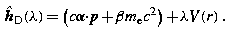
With this restriction on the 4-potential, Dirac's Hamiltonian becomes

(22.87)

Consider stationary solutions with energy E satisfying

Since is invariant with respect to rotation about r = 0, it commutes with the generators J ₁, J ₂, J ₃ mentioned in Sect. 22.1.1, corresponding to components of the total angular momentum j of the electron, usually decomposed into an orbital part l and a spin part s,

(22.88)

where

Eigenstates of Angular Momentum

We can construct simultaneous eigenstates of the operators j ² and j ₃ by using the product representation of the rotation group SO(3), which is reducible to the Clebsch-Gordan sum of two irreps

(22.89)

We construct a basis for each irrep from products of basis vectors for and respectively. is a 2-dimensional representation spanned by the simultaneous eigenstates ϕ _σ of s ² and s ₃

for which we can use 2-rowed vectors

The representation is (2l + 1)-dimensional; its basis vectors can be taken to be the spherical harmonics

so that

We shall assume that spherical harmonics satisfy the standard relations

where l _±= l ₁ ± l ₂, so that

(22.90)

Basis functions for the representations with have the form (The order of coupling is significant, and great confusion results from a mixing of conventions. Here we couple in the order l, s, j. The same spin-angle functions are obtained if we use the order s, l, j but there is a phase difference (− 1)^l−j+1/2 = (− 1)^(1−a)/2. You have been warned!)

(22.91)

where is a Clebsch-Gordan coefficient with

Inserting explicit expressions for the Clebsch-Gordan coefficients gives

(22.92)

The vectors (22.92) satisfy

(22.93)

The parity of the angular part is given by (− 1)^l, with the two possibilities distinguished by means of the operator

(22.94)

so that

The basis vectors are orthonormal on the unit sphere with respect to the inner product

(22.95)

Eigenstates of Dirac Hamiltonian in Spherical Coordinates

Eigenstates of Dirac's Hamiltonian (22.87) in spherical coordinates with a spherically symmetric potential V(r) = eϕ(r),

(22.96)

are also simultaneous eigenstates of j ², of j ₃ and of the operator

(22.97)

where K′ is defined in (22.94) above. Denote the corresponding eigenvalues by j, m and κ, where

(22.98)

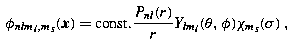
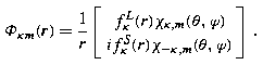
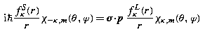
Then the simultaneous eigenstates take the form

(22.99)

where κ =− (j + 1/2)a is the eigenvalue of K′, and the notation χ _κ,m replaces the notation χ _j,m,a used previously in (22.91). The factor i in the lower component ensures that, at least for bound states, the radial amplitudes P _Eκ (r), Q _Eκ (r) can be chosen to be real. This decomposition into radial and angular factors exploits the identity

(22.100)

and gives a reduced eigenvalue equation

(22.101)

Angular Density Distributions

It is a remarkable fact that the angular density distribution

(22.102)

where m =− j,− j + 1,… , j − 1, j, is independent of the sign of κ; the equivalence of

and

where μ =  cos θ, was demonstrated by Hartree [22.19].

Angular densities for the lowest |κ| values are given in Table 22.1. The corresponding nonrelativistic angular densities

are listed in Table 22.2.

Table 22.1 Relativistic angular density functions

Table 22.2 Nonrelativistic angular density functions

Radial Density Distributions

The probability density distribution ρ _Eκm (r) associated with the stationary state (22.99) is given by

(22.103)

Since A _κ,m does not depend on the sign of κ, the angular part can be factored so that

where

(22.104)

defines the radial density distribution.

Subshells in j-j Coupling

The notion of a subshell depends on the observation that the set {ψ _E,κ,m , m =− j,… , j} have a common radial density distribution. The simplest atomic model is one in which the electrons move independently in a mean field central potential. Since

(22.105)

a state of 2j + 1 independent electrons, with one in each member of the set {ψ _E,κ,m , m =− j,… , j}, has a spherically symmetric probability density. If E belongs to the point spectrum of the Hamiltonian, then (22.105) gives a distribution localized in r, and we refer to the states {E, κ, m}, m =− j,… , j as belonging to the subshell {E, κ}.

The notations in use for Dirac central field states are set out in Table 22.3. Here l is associated with the orbital angular quantum number of the upper pair of components and with the lower pair. Note the useful equivalence

Defining we have also .

Table 22.3 Spectroscopic labels and angular quantum numbers

Radial Amplitudes

Textbooks on quantum electrodynamics usually contain extensive discussions of the formalism associated with the Dirac equation but rarely go beyond the treatment of the hydrogen atom Chapt. 10. Greiner's textbook [22.4] is an honorable exception, with many worked examples. A more exhaustive list of problems in which exact solutions are known is contained in [22.20]; it is particularly rich in detail about equations of motion and Green's functions in external electromagnetic fields of various configurations; coherent states of relativistic particles; charged particles in quantized plane wave fields. It also incorporates discussion of extensions of the Dirac equations due to Pauli which include explicit interaction terms arising from anomalous magnetic or electric moments.

Atoms and molecules with more than one electron are not soluble analytically so that numerical models are needed to make predictions. The solutions are sensitive to boundary conditions on which we focus in this section. For large r, solutions of (22.101) can be found proportional to exp (± λr), where

(22.106)

Thus λ is real when − c ² ≤ E ≤ c ², and pure imaginary otherwise.

Singular Point at r = 0

Singularities of the nuclear potential near r = 0 have a major influence on the nature of solutions of the Dirac equation. Suppose that the potential has the form

(22.107)

so that Z(r) is the effective charge seen by an electron at radius r from the nuclear center. The dependence of Z(r) on r may reflect the finite size of the nuclear charge distribution, so far treated as a point, or the screening due to the environment. Assume that Z(r) can be expanded in a power series of the form

(22.108)

in a neighborhood of r = 0. This property characterizes a number of well-used models

• 1. Point nucleus: Z ₀ ≠ 0; Z _n  = 0,  n > 0.

• 2. Uniform nuclear charge distribution:

  

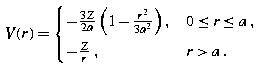  (22.109)

  This gives the expansion Z ₀ =− 3Z/2a, Z ₁ = 0, Z ₂ =+ Z/2a ³, Z _n  = 0 for n > 2 when r ≤ a.

• 3. Fermi distribution: The nuclear charge density has the form

  

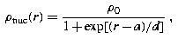
  where ρ ₀ is chosen so that the total charge on the nucleus is Z.

Other nuclear models, reflecting the density distributions deduced from nuclear scattering experiments, can be found in the literature.

Series Solutions Near r = 0

Any solution for the radial amplitudes of Dirac's equation in a central potential

(22.110)

with radial density

can be expanded in a power series near the singular point at r = 0 in the form

(22.111)

where

and γ, p _k , q _k are constants which depend on the nuclear potential model.

Point Nuclear Models

For a Coulomb singularity, Z ₀ ≠ 0, the leading coefficients satisfy

(22.112)

so that

(22.113)

Finite Nuclear Models

Finite nuclear models, for which Z ₀ = 0, have no singularity in the potential at r = 0. The indicial equation (22.113) reduces to γ =± |κ|, so that for κ < 0,

(22.114)

(22.115)

with

and for κ ≥ 1,

(22.116)

(22.117)

with

In both cases the solutions consist of either purely even powers or purely odd powers of r, contrasting strongly with the point nucleus case, where both even and odd powers are present in the series expansion.

The Nonrelativistic Limit

For a solution linked to a nonrelativistic state with orbital angular momentum l, one expects the nonrelativistic limit

The limiting behavior reveals some significant features.

Finite nuclear models

The behavior is entirely regular:

Point nuclear models

Since

(22.113) shows that the leading coefficient p ₀ vanishes in the limit so that,

(22.118)

All higher powers of odd relative order vanish in the limit for both components. The behavior in the case κ < 0 is entirely regular.

Square Integrable Solutions

Square integrable solutions require ∫ D _E,κ (r)dr to be finite; since the solutions are smooth, except possibly near the singular endpoints r → 0 and r →∞, we focus on the behavior at the endpoints:

r →∞

For real values of λ the condition

requires that P _Eκ (r), Q _Eκ (r) are proportional to exp (− λr) with λ > 0.

This means that bound states can only exist when E lies in the interval − c ² ≤ E ≤ c ². Outside this interval solutions are necessarily of scattering type and so

diverges when |E| > c ².

r → 0

This limit requires

Since D _E,κ (r) ∼ r ^±2γ as r → 0, this condition holds when . Only the solution with γ > 0 satisfies the condition when , or , and the solution with γ < 0 must be disregarded. This corresponds to the limit point case of a second-order differential operator [22.21]. In the special case |κ| = 1 or this limits Z to be smaller than . For , both solutions are square integrable near the origin (the limit circle case) and the differential operator is no longer essentially self-adjoint.

The Coulomb potential must have a finite expectation for any physically acceptable solution, so that we also require

This is always satisfied by the solution with γ > 0 for all |Z| < α ⁻¹ |κ|, but not by the solution with γ < 0. Imposing this condition restores essential self-adjointness (on a restricted domain) for 118 < Z ≤ 137.

Hydrogenic Solutions

The wave functions for hydrogenic solutions of Dirac's equation are presented in Sect. 22.8.2. Here we note some properties of hydrogenic solutions that reveal dynamical effects of relativity in the absence of screening by orbital electrons. In this case Z ₀ = Z, Z _n  = 0, n > 0. When − c ² < E < c ² we have bound states. The parameter λ, (22.106), can conveniently be written

(22.119)

so that rearranging (22.106) gives

(22.120)

essentially equivalent to Sommerfeld's fine structure formula. In the formal nonrelativistic limit, c →∞, we have

so that N is closely related to the principal quantum number, n, appearing in the Rydberg formula. As in Sect. 22.8.2, we write ρ = 2λr.

Define the inner quantum number

Substitute for E from (22.120) to get

(22.121)

where n = n _r + |κ| is the principal quantum number, the exact equivalent of the principal quantum number of the nonrelativistic state to which the Dirac solution reduces in the limit c →∞. With this notation, the radial amplitudes for bound hydrogenic states are

(22.122)

(22.123)

where

is the normalization constant. For definitions of the confluent hypergeometric functions M(a, b;c;z) see [22.22, Sect. 13.1].

Table 22.4 lists expectation values of simple powers of the radial variable ρ = 2Zr/N from [22.23] and [22.24]. Simple algebra, using the inequalities γ < |κ| and N < n, yields the inequality

the inequality is reversed for s < 0. In the same way, it is easy to deduce that relativistic hydrogenic eigenvalues lie below the nonrelativistic eigenvalues

Thus, in the absence of screening, Dirac orbitals both contract and are stabilized with respect to their nonrelativistic counterparts. The relativistic and nonrelativistic expectation values approach each other as the relativistic coupling constant, Z/c = αZ → 0. This formal nonrelativistic limit is approached as α → 0 or c →∞, in which the speed of light is regarded as infinite.

Table 22.4 Radial moments 〈ρ ^s〉

The Free Electron Problem in Spherical Coordinates

The radial equation (22.101) for the free electron (V(r) = 0) gives a pair of first order ordinary differential equations

(22.124)

from which we deduce that

(22.125)

where p ² = m ² c ² − E ²/c ² = p. p and the angular quantum numbers κ and are associated respectively with the upper and lower components. These are defining equations of Riccati-Bessel functions [22.22, Sect. 10.1.1] of orders l and respectively, where

Thus the solutions of (22.125) are functions of the variable x = pr of the form

where the ratio of A and B is determined by (22.124) and where f _l (x) is a spherical Bessel function of the first, second or third kind [22.22, Sect. 10.1.1]. Thus

(22.126)

Equations (22.124) require that Riccati-Bessel solutions of the same type be chosen for both components. The possibilities are:

Standing Waves

The two solutions of the same type are f _l (x) = j _l (x),  f _l (x) = y _l (x). The j _l (x) are bounded everywhere, including the singular points x = 0,  x →∞ and have zeros of order l at x = 0. The y _l (x) are bounded at infinity but have poles of order l + 1 at x = 0.

Progressive Waves

The spherical Hankel functions (functions of the third kind) are linear combinations

Recalling that p is real if and only if |E| > mc ², we see that h _l ⁽¹⁾(x), h _l ⁽²⁾(x) are bounded as x →∞ and have poles of order l + 1 at x = 0. Notice that when |E| < mc ², which does not occur for a free particle, p becomes pure imaginary and no solution exists which is finite at both singular points.

The normalization constant can be determined by using the well-known result

The choice ensures that

Noting that

and dp/dE = c ² p/E gives

when .

Numerical Approximation of Central Field Dirac Equations

The main drive for understanding methods of numerical approximation of solutions of Dirac's equation comes from their application to many-electron systems. Approximate wave functions for atomic or molecular states are usually constructed from products of one-electron orbitals, and their determination exploits knowledge gained from the treatment of one-electron problems. Whilst the numerical methods described here are strictly one-electron in character, extension to many-electron problems is relatively straightforward.

Finite Differences

The numerical approximation of eigensolutions of the first order system of differential equations (22.101)

(22.127)

can be achieved by more or less standard finite difference methods given in texts such as [22.25]. For states in either continuum, E > mc ² or E <− mc ², the calculation is completely specified as an initial value problem for a prescribed value of E starting from power series solutions in the neighborhood of r = 0. Solutions of this sort exist for all values of (complex) E except at the bound eigensolutions in the gap − mc ² < E < mc ². For bound states, the calculation becomes that of a two-point boundary value problem in which the eigenvalue E has to be determined iteratively along with the numerical solution. We concentrate on the latter, which is more involved.

It is convenient to write

(22.128)

so that ϵ approaches the nonrelativistic eigenvalue in the limit c →∞. For the one-electron problem, (22.101) can be written in the general form

(22.129)

where u(s) and χ(s) are two-component vectors, such that

and r(s) is a smooth differentiable function of a new independent variable s. This facilitates the use of a uniform grid for s mapping onto a suitable nonuniform grid for r. Common choices are

for suitable values of the parameters r ₀ and h, and

where A is a constant, chosen so that the spacing in r _n increases exponentially for small values of n and approaches a constant for large values of n. The exponentially increasing spacing is appropriate for tightly bound solutions, but a nearly linear spacing is advisable to ensure numerical stability in the tails of extended and continuum solutions.

The most convenient numerical algorithm involves double shooting from s ₀ = 0 and s _N  = Nh towards an intermediate join point s = Jh, adjusting ϵ until the trial solutions have the right number of nodes and have left- and right-limits at s = Jh which agree to a pre-set tolerance (commonly about 1 part in 10⁸).

The deferred correction method [22.26,27] allows the precision of the numerical approximation to be improved as the iteration converges. Consider the simplest implicit linear difference scheme for the first order system

based on the trapezoidal rule of quadrature, is

(22.130)

which has a local truncation error O(h ²). The precision can be improved, at the expense of increasing the computational cost per iterative cycle, by adding higher order difference terms to the right-hand side in (22.130). Use of the trial solution from the previous cycle leaves the stability properties of (22.130) are unaltered, but the converged solution has much higher accuracy.

To apply this to the Dirac system, write f(s) = dr/ds and

Also consider a slightly generalized problem in which V(r) is replaced by a discretized potential U _j ^(ν) that may change from one iteration to the next as in a self-consistent field calculation. The first iteration is

(22.131)

where superscript 0 refers to initial estimates and superscript 1 to the result of the first iteration. On the (ν + 1)-th iteration, we solve

(22.132)

where δ ³  U _j+1/2 ^(ν) is the central-difference correction of order 3 [22.22, Sect. 25.1.2]. Higher order difference corrections (at least to order 5) are included in modern codes to improve the accuracy and numerical stability of weakly bound solutions. This deferred correction algorithm can be shown to converge asymptotically to the required solution of the differential system with a local truncation error of order when difference corrections of order 2p + 1 are employed [22.28].

Expansion Methods

Methods of solving the Dirac equation which represent the one-electron wave function as a linear combination of sets of square integrable functions (basis sets) have become popular in the last 10 years. Simple and rigorous criteria for choosing effective basis sets for this purpose are now available, and classes of functions that satisfy these criteria are known. Consequently, cheap and accurate calculations of the electronic structure of atoms and molecules are now a practical possibility.

Finite difference algorithms generate eigensolutions one at a time. Basis set methods replace the differential operator of (22.87) with a finite symmetric (in some cases complex Hermitian) matrix of dimension 2N. The spectrum of this operator, which is of course a pure point spectrum, consists of three pieces: N eigensolutions with E <− mc ² (ϵ <− 2mc ²) representing the eigenstates of the lower continuum; N _b < N eigensolutions in the gap − mc ² < E < mc ² (− 2mc ² < ϵ < 0) corresponding to bound states; and N − N _b eigensolutions with E > mc ² (ϵ > 0) representing the eigenstates of the upper continuum. For properly chosen basis sets, the approximation properties of bound state eigensolutions are similar to those of the equivalent nonrelativistic eigensolutions. Solutions at continuum energies have the correct behavior near r = 0, but their amplitudes decrease exponentially like bound state solutions at large values of r. The criteria on which this description rests are as follows:

• A. The eigenstates of are 4-component central field spinors whose components are coupled. The basis functions should therefore also consist of 4-component spinors of the form

  

  (22.133)

• B. The spinor basis functions should, as far as practicable, satisfy the boundary conditions near r = 0 of Sect. 22.5.3. They should also be square integrable at infinity.

• C. Acceptable spinor basis functions should satisfy the relation

  

  (22.134)

  in the nonrelativistic limit, c →∞.

• D. Acceptable spinor basis functions must have finite expectation values of component operators of , namely α  ⋅  p, β and V(r).

Finite Basis Set Formalism

Assume that each solution of the target problem is approximated as a linear combination

(22.135)

where c ^L _κj , c ^S _κj   j = 1⋯N, are arbitrary constants, so that each j-term on the right-hand side has the form (22.133). This enables us to construct a Rayleigh quotient

(22.136)

where both and 〈ψ|ψ〉 are quadratic expressions in the expansion coefficients c ^L _j , c ^S _j . By requiring that W[ψ] shall be stationary with respect to arbitrary variations in the expansion coefficients, we arrive at the matrix eigenvalue equation

(22.137)

where the matrix Hamiltonian is denoted by

c ^L _κ , c ^S _κ are N-vectors, and V ^LL _κ , V ^SS _κ , S ^LL _κ , S ^SS _κ , Π ^LS _κ and Π ^SL _κ are all N × N matrices. Using superscripts T to denote either of the letters L, S, the elements of the matrices are defined by

(22.138)

(22.139)

and

(22.140)

(22.141)

If f ^L _iκ (r) and f ^S _iκ (r) vanish at both r = 0 and r →∞, then a simple integration by parts shows that Π ^LS _κ and Π ^SL _κ are Hermitian conjugate matrices.

Physically Acceptable Basis Sets

The four criteria described above are exploited in the following way:

• 1. The structure of (22.133) ensures (i) that the upper and lower components have properly matched angular behavior. It also emphasizes that the radial parts are part of a spinor structure which should be kept intact when making approximations.

• 2. The nuclear singularity drives the dynamics of the electronic motion. It is therefore important that approximate trial solutions should have the correct analytic character as defined in Sects. 22.5.3 and 22.5.4. An expansion of f ^L _iκ (r) and f ^S _iκ (r) at r = 0 must reproduce this analytic behavior exactly if the approximation is to be physically reliable. The boundary conditions are part of the definition of a quantum mechanical operator; changing them gives a different operator with a different eigenvalue spectrum, so that trial functions which do not satisfy the boundary conditions of the physical problem cannot reproduce the physical solution. The behavior as r →∞ is less crucial. Provided a bound wavefunction is well approximated over the region containing most of the electron density, the results are insensitive to many choices.

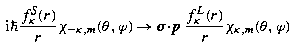
• 3. The correct reduction of the Dirac equation to Schrödinger's equation in the nonrelativistic limit (for example see [22.4, p. 97]) depends upon the operator identity

  

  In the basis set formalism, the matrix equivalent of this equation is

  

  (22.142)

  where

  

  is the ij-element of the nonrelativistic radial kinetic energy matrix. This is not true in general unless criterion C holds [22.29,30]. The criterion can only be satisfied by matched pairs of functions f ^L _iκ (r), f ^S _iκ (r), ruling out all choices of basis set in which large and small components are not matched in pairs. Another way of viewing this result is to observe that for a general basis set, the sum over intermediate states in (22.142) is necessarily incomplete. The Hermitian conjugacy property, Π ^LS _κij  = Π ^SL _κji ensures that the omitted terms give real and non-negative contributions. Thus all other choices of basis set cause (22.142) to underestimate the nonrelativistic kinetic energy [22.29] and to give spuriously large relativistic energy corrections.

  We emphasize that (22.134) need only be true in the limit c →∞; however, basis sets used for finite values of c should be smooth functions of c ⁻¹ as c →∞ so that the equality

  

  (22.143)

  holds in the limit.

• 4. This ensures that the basis functions are in the domain of the Dirac operator; the meaning of this statement can be made precise in a functional analytic discussion such as in [22.3]. Some implications for the finite basis set approach are given in the author's paper [22.15, pp. 235-253], which discusses the convergence of expectation values of operators for approximate Dirac wavefunctions obtained by this method. Here the main importance is that a (possibly singular) multiplicative operator V(r) (say, − Z/r) has N × N matrices V ^LL _κ , V ^SS _κ with finite elements. This must be true both for exact solutions and for approximations if the wave functions are to represent physical states. In particular, both matrices must have a lowest eigenvalue V _min ^(N) say. Consider now the quantity , where

  

  With λ = 0 we have a free Dirac particle with a two-branched continuous spectrum E > mc ² and E <− mc ². A negative definite V(r) has always (ψ|V(r)|ψ) > V _min; clearly,

  

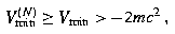  (22.144)

  for all values of N. So if we increase λ from 0 to 1, the eigenvalues of trial solutions corresponding to eigenvalues in the upper continuum at λ = 0 will be smoothly decreasing functions of λ bounded below by V _min for all values of N. It follows that the upper set of eigenvalues has a fixed lower bound in the gap for each finite matrix approximation. If the basis set satisfies suitable completeness criteria in an appropriate Hilbert space as N →∞ (see [22.15, pp. 235-253], [22.31] for more details) we see that, if (22.144) holds for all values of N, the infinite sequence {E _N+i ^(N),  N = N ₀, N ₀ + 1,…} of eigenvalues approximating the ith bound state has a finite lower bound, and therefore, by the completeness of the real numbers, it must have a limit point E _i in the bound state gap . Thus Rayleigh-Ritz approximations for Dirac's Hamiltonian converge in the same fashion as the corresponding nonrelativistic Rayleigh-Ritz approximations [22.30,31].

Catalogue of Basis Sets for Atomic Calculations

A. L-Spinors:

L-spinors [22.31] are related to Dirac hydrogenic functions in much the same way as Sturmian functions [22.32,33] are related to Schrödinger hydrogenic functions (Sect. 22.3). They are solutions of the differential equation system

(22.145)

where x = 2λr is a scaled radial coordinate, with fixed λ which can be related to an energy parameter , and μ ², a root of the equation μ ⁴ − 2cμ ²/λ + 1 = 0, is given by

(22.146)

This choice ensures that tends smoothly to the corresponding Coulomb Sturmian in the nonrelativistic limit c →∞ [22.31]. L ² boundary conditions are satisfied if ; when , then respectively coincide with the Dirac-Coulomb eigenfunctions P _nκ (r) and Q _nκ (r) having principal quantum number n = n _r + |κ|. The explicit form for L-spinors, in terms of Laguerre polynomials (see Sect. 9.03.02), , is

(22.147)

(22.148)

where

(22.149)

is chosen so that the diagonal elements of the Gram (or overlap) matrix are unity for both large and small components. Both Gram matrices are tri-diagonal with non-zero off-diagonal elements

(22.150)

where T = L, S, η ^L =− 1 and η ^S =+ 1. This convention facilitates the construction of the blocks of the matrix Hamiltonian (22.137), which are banded when the operators are the powers r ⁿ, n >− 1. The properties of Laguerre polynomials ensure that the matrix of the Coulomb potential is diagonal. For a full discussion of L-spinors, their orthogonality and completeness properties, and applications to hydrogenic atoms see [22.31].

L-spinors are most useful for hydrogenic problems, either for isolated atoms or for atoms in strong electromagnetic fields (see Chapt. 13). The equivalent nonrelativistic Coulomb Sturmians have for a long time been used to study the Zeeman effect on high Rydberg levels, especially in the region where chaotic behavior is expected [22.34] (see Chapt. 15).

B. S-Spinors:

S-spinors have the functional form of the most nearly nodeless L-spinors characterized by the minimal value of n _r, and can be viewed as the relativistic analogues of Slater functions (STOs). When κ is negative, take n _r = 0, so that

When κ is positive, we must take n _r = 1, and then

These can be simplified by inserting the explicit expressions L ₀ ^(2γ)(x) = 1, L ₁ ^(2γ)(x) = 2γ + 1 − x. We define a set of S-spinors with exponents {λ _m , m = 1, 2,… , N} by rewriting the above in the form

(22.151)

where T = L, S, ,

(22.152)

and

The choice of the set of positive real exponents {λ _m , m = 1, 2,… , N}, must be such as to assure Rayleigh-Ritz convergence [22.15, pp. 235-253)] and to maximize the rate at which it is attained. In particular, if one particular exponent is chosen to have the value , then the corresponding S-spinor is a true hydrogenic solution. In this case the trial solution is exact. Clearly, S-spinors inherit desirable properties of L-spinors and, in particular, satisfy criteria A-D.

All elements of the matrix Hamiltonian of the Dirac hydrogenic problem can be expressed in terms of Euler's integral for the gamma function [22.22, Sect. 6.1.1]:

and are therefore readily written down and evaluated. The effectiveness of this method depends upon the choice of exponent set: see D below. We refer to calculations using this scheme for many-electron systems in Sect. 22.7.

C. G-Spinors:

The G-spinors are the relativistic analogues of nonrelativistic spherical Gaussians (SGTO), popular in quantum chemistry for studying the electronic structure of atoms and molecules. They satisfy the relativistic boundary conditions for a finite size nuclear charge density distribution at r = 0, and are therefore the most convenient for relativistic molecular electronic structure calculations. They are defined so that (22.143) holds for finite c as well as in the nonrelativistic limit, which is equivalent to

(22.153)

Thus, if

(22.154)

(22.155)

Note that the leading term in (22.155) vanishes when κ < 0, so that the radial amplitude r ⁻¹ f ^(S) _m (r) is never singular, even in the s-state case when κ =− 1, l = 0.

D. Exponent Sets for S- and G-Spinors:

Quantum chemists are familiar with the use of nonrelativistic STO and GTO basis sets, and there are extensive collections of optimized exponents which permit economical calculations for atomic and molecular calculations [22.35,36,37]. These sets are a good starting point for relativistic calculations also. By and large, the compilations ignore mathematical completeness, which although desirable is unattainable in practice. However, basis sets can almost always be constructed to give adequate numerical precision for most purposes.

An effective alternative to optimization, especially for atoms, is to use geometrical sequences {λ _m } of the form

(22.156)

which depend upon just two parameters α _N , β _N . A convenient way to do this is to find a pair for small N ₀, say N ₀ = 9, in a cheap and simple nonrelativistic calculation and then to increase N systematically using relations such as

where a, b are positive constants. Experience shows that no linear dependence problems (caused by ill-conditioning of the S ^T matrices) are encountered when β _N  > 1.2 for S-spinors, with N up to about 30, or β _N  > 1.5 for G-spinors with N up to about 50.

E. Other Types of Analytic Basis Sets; Variational Collapse:

The earliest work with atoms [22.38,39] used STO functions of the form {r ^γ exp (− λ _m r),  m = 1,… N} for both large and small components, whilst Kagawa [22.40,41] used integer powers instead of the noninteger γ. Drake and Goldman [22.42] used functions of the form {r ^γ+i exp (− λr), i = 0,… N − 1}. For hydrogenic problems, these worked well for negative κ states, but gave a single spurious eigenvalue for positive κ, which could be simply deleted from the basis set. Various test calculations are included in the review article [22.43, Sect. IV]. Other attempts to use GTOs in the early 1980's led to problems interpreted as a failure of the Rayleigh-Ritz method because of the presence of “negative energy states” with a spectrum unbounded below: so-called “variational collapse”. It is clear that all these approaches fail to observe three, and sometimes all, of the four criteria for acceptable basis sets. They are incapable of satisfying the physical boundary conditions, and it is therefore hardly surprising that they give unphysical spectra.

Several procedures have been advocated to overcome the problem, of which the two most popular are “kinetic balance” and projection operators. Kinetic balance, suggested by Lee and McLean [22.44], advocates augmenting a GTO basis, common to both large and small components, with additional functions to “balance the set kinetically”. This appears to “fix up” the problem for the upper spectrum, but introduces spurious states, mainly in the lower part of the spectrum, as well as increasing the size of the small component basis set. There is no rigorous nonrelativistic limit, and no mathematical proof of convergence such as that guaranteed by criteria A-D. A model with spurious negative energy states cannot furnish a consistent physical interpretation of negative energy solutions as positron states, expected of a proper relativistic theory.

If “variational collapse” is attributed to the absence of a lower bound to the Dirac spectrum as a whole, the idea of introducing a projection operator to eliminate collapse seems attractive. This is easy to do for free electrons, where the operators

select positive/negative energy solutions. Unfortunately, this cannot be done in the presence of a potential except by an approximation which complicates calculations and reduces the efficiency of algorithms. The “negative energy sea” also depends upon the choice of potential; perturbing the potential (as long as it does not change the domain of the Hamiltonian) induces a unitary transformation taking one set of eigenstates into another which inevitably mixes the old positive and negative energy states. For example a relativistic calculation on a hydrogenic atom in which the nuclear charge is perturbed gives incorrect answers if the negative energy contribution to the perturbation series is omitted [22.45].

In any event, the finite matrix eigensolutions include both positive energy and negative energy states. It is therefore a simple matter to exclude the negative energy states if their contribution is expected to be negligible; this is the no virtual-pair approximation. The negative energy solutions are inert spectators for most atomic processes, just as are those positive energy solutions which lie deep in the atomic core. It is easy to go beyond the no virtual-pair approximation if the physical problem demands it.

Finite Element Methods:

Johnson et al. [22.46,47], following earlier work on relativistic ion-ion collisions by Bottcher and Strayer [22.48], popularized the use of a basis of B-splines in relativistic atomic calculations. See Sect. 8.1.1. The method has mainly been of use in relativistic many-body calculations on the spectra of heavy ions. See Sect. 21.6 for spline-Galerkin representations in nonrelativistic atomic structure, such as [22.49]. Parpia and Fischer explored the spline-Galerkin approach for the Dirac equation [22.50], but this method has not been extended so far to relativistic many-electron atoms.

Many-Body Calculations

Atomic States

The construction of atomic many-electron wave-functions from products of central field Dirac orbitals is employed to simplify the algorithms for calculating electronic structures and properties. This can be either in the context of expansions in Slater determinants of the traditional type, or by use of Racah algebra. A complete description of the methods of the latter sort used in popular computer codes is found in [22.27, Sect. 2].

Slater Determinants

An antisymmetric state of N independent electrons in configuration space can be constructed in the form

(22.157)

This Slater determinant is an antisymmetric eigenfunction of H ₀ corresponding to the energy and of the angular momentum projection corresponding to the eigenvalue . Defining the parity of a Dirac electron orbital as that of its upper component, , we see that this has parity .

Configurational States

Configurational state functions (CSF) having specified total angular momentum J and parity Π can be constructed by vector addition of the individual angular momenta: . We write such states as

(22.158)

where is a generalized Clebsch-Gordon coefficient, and γ defines the angular momentum coupling scheme.

A list of orbital quantum numbers, {α ₁, α ₂,… , α _N } defines an electron configuration. If the configuration belongs to a single subshell, then the states share a common set of labels {n, κ} where n is the principal quantum number. In j − j coupling, the α-subshell states of N _α equivalent electrons can therefore be identified (we can suppress the projection M _α and the parity Π _α ) by the labeling , γ _α , J _α , where γ _α distinguishes degenerate states of the same J _α . For j − j coupling, such labels are needed only for ; the seniority scheme, [22.27, Sects. 2.3, 2.4)], provides a complete classification for . A list of states of configurations j ^N, classified in terms of the seniority number v and of total angular momentum J, appears in Table 22.5.

Table 22.5 j ^N configurational states in the seniority scheme. The multiplicity of each unresolved degenerate state is indicated by a superscript

CSF Expansion

Atomic state functions (ASF) are linear superpositions of CSF's, of the form

(22.159)

where c _α are a set of (normally) real coefficients. These coefficients are usually chosen so that Ψ(γΠJ) is an eigenstate of the many-electron Hamiltonian matrix in a finite subspace of CSF's.

Matrix Element Construction

A full presentation of the reduction of matrix elements between CSF's to computable form is beyond the scope of this chapter. There are two approaches: one is based on expanding all CSF's and ASF's in Slater determinants, whilst the other exploits the properties of central field orbital spinors. The principles underlying the first are straightforward and may be found in atomic physics texts and review articles such as [22.26,27].

The use of second quantization and diagrammatic methods of the quantum theory of angular momentum provides a powerful means of reducing matrix elements between atomic CSF's to a linear combination of radial integrals in a systematic way. The method, which is fully explained in [22.27], leads to a complete classification of matrix element expressions for all the one- and two-electron operators treated in this chapter. A full implementation within the j − j coupling seniority scheme is available in various versions of the GRASP code [22.51,52,53].

Dirac-Hartree-Fock and Other Theories

The notation above echoes that of the nonrelativistic theory of Chapt. 21, and it is possible to proceed along similar lines.

Dirac-Hartree-Fock Theory

Dirac-Hartree-Fock theory works exactly as described in Sect. 21.4; relativistic counterparts of Koopmans' theorem, fixed-core approximations, Brillouin's theorem are easy to obtain. The properties of Dirac-Hartree-Fock functions closely resemble those of Hartree-Fock functions, though allowance must be made for the fact that, for example, np orbitals (with ) and orbitals (with ) have different spatial distributions as a consequence of the dynamical and indirect effects of relativity. For further insight see [22.23,26].

Most such calculations are currently made with updated versions of the codes of Desclaux [22.54] or Grant [22.51,52,53] which rely on finite difference methods resting on the techniques of Sect. 22.6.1. Further details may be found in the code descriptions.

Finite Matrix Methods for Atoms and Molecules

In view of the rapid pace of development of finite matrix methods, especially for the treatment of relativistic molecular electronic structure in the Born-Oppenheimer (fixed nucleus) approximation, it seems appropriate to give a brief outline of the extension of the one-electron equations of Sect. 22.4.2 to the many-electron case.

The method of approximation generalizes the one-body approximation scheme of Sect. 22.6.2 to the many-body problem based on the effective Hamiltonian of Sect. 22.4.1. This leads to an energy functional of the form

(22.160)

where E ₀ is the expected value of H ₀ (22.76) and E ₁ the expected value of H ₁ for the finite basis many-body trial function. This leads to matrix Dirac-Fock equations of the form

(22.161)

In general, the Fock matrix F is a sum of several matrices

(22.162)

where, for each symmetry κ and nuclear center, A, of the molecule, f can be partitioned into blocks

(22.163)

The matrix

(22.164)

is the matrix of the Coulomb repulsion part of the electron-electron interaction and

(22.165)

is the matrix of the Breit interaction.

In the atomic (one nuclear center) case, following [22.55], these matrices can also be blocked by symmetry κ. Using superscripts T to label the L or S components, and the notation to denote the complementary label: when T = L or when T = S, then the direct Coulomb part J ^TT _κ has matrix elements

(22.166)

whilst the exchange part has the form

(22.167)

where TT′ denotes any combination of component labels. Here is a density matrix with elements

(22.168)

where c _κp ^T are the expansion coefficients. The Breit interaction matrices have the similar form

(22.169)

and

(22.170)

The matrix elements are constructed from standard radial integrals

(22.171)

where

Similarly

(22.172)

and

(22.173)

Further details about the coefficients b _ν (jj′), e _ν (jj′), d _ν (κκ′) and g _ν (κκ′) may be found in [22.55].

This formalism has been implemented for closed shell atoms with both S-spinors and G-spinors [22.55]. Computational aspects of calculating the radial integrals using S-spinors are discussed in [22.56,57], and can be adapted with relatively small modifications to G-spinor basis sets. As yet, there have been relatively few applications by comparison with codes based on finite difference methods, but the potential can be gauged from papers such as [22.55,58,59,60,61], which deal with Dirac-Fock and Dirac-Fock-Breit calculations, many-body perturbation theory and coupled-cluster schemes.

G-spinor basis sets provide the most promising technique for application to the electronic structure of molecules; computer codes are under active development.

Electron Correlation in Atomic Calculations

Here we use the term correlation to denote methods which go beyond the single determinant approximation of Dirac-Hartree-Fock theory. These include configuration interaction schemes, in which each ASF is represented as a linear combination of CSF's built from previously determined orbital spinors and multiconfiguration Dirac-Fock calculations in which the orbitals are optimized simultaneously. Calculations representative of state of the art techniques will be found in [22.62,63].

Many-body perturbation theory calculations and coupled-cluster calculations are not well suited to calculations with finite difference codes, because of the expense of calculating more than a limited orbital basis and all the matrix elements required. Calculations based on finite matrix methods enable this sort of calculation to be done more economically. Some justification for the use of finite matrix methods in relativistic many-body theory is given in [22.15, pp. 235-253].

The relativistic version of quantum defect theory [22.64,65] also gives insight into the competing roles of relativistic dynamics and screening in atoms. Compared with nonrelativistic quantum defect theory, it has been under-used.

Radiative Corrections

The term “radiative corrections” is usually interpreted to mean QED contributions to energies, expectation values or rates of atomic or molecular processes that arise from interaction between the electron-positron and photon fields, apart from those directly attributable to the nonrelativistic Coulomb interaction. This includes the relativistic and retardation effects embodied in the effective interaction between electrons as well as contributions from processes that are not so included. We consider two such processes, the electron self-energy and the vacuum polarization, which involve interactions of the same formal order as those giving rise to the covariant electron-electron interaction discussed above, but which are formally infinite. These are the lowest order processes requiring renormalization. See [22.7,8,10,15] for more details.

Electron Self-Energy

For a one-electron system, the renormalized expression for the self-energy of an electron in the state a in Feynman gauge is

(22.174)

where

This represents the contribution from virtual processes involving the exchange of a single photon. The photon propagator has been modified to give the photon and effective mass Λ, so that the denominator of (22.69) becomes q ² − Λ ² + iδ. The two parts of this formula diverge as Λ →∞, though the limit of their difference is finite. This makes calculation difficult and expensive. There are several approaches:

• 1. For atomic number Z ≲ 20, an expansion in powers of the electron-nucleus coupling parameter αZ = Z/c is satisfactory.

• 2. At larger atomic numbers an expansion in αZ evidently fails to converge, and nonperturbative methods must be sought. This too is computationally difficult and expensive. The results for hydrogenic ions have been tabulated [22.66] for atomic numbers in the range 1 ≤ Z ≤ 100. (See [22.10, Chapt. 2] for an up-to-date summary biased towards applications to the spectroscopy of highly-ionized atoms.)

• 3. Processes involving more than one virtual photon are hard to calculate, and have mostly been ignored. See [22.10] for references.

Vacuum Polarization

The contribution of vacuum polarization is next in order of importance in the list of radiative corrections in atoms. As shown by (22.49), the nuclear potential generates a current in the vacuum that is responsible for a short-range screening of the nuclear charge. This can be represented as a local perturbing potential which is easy to take into account [22.67,68,69].

Radiative Processes

The operator j ^μ(x)A _μ (x) which occurs in the interaction Hamiltonian (22.61) describes processes in which the number of photons present can increase or decrease by one. The Fock space operator may be written

(22.175)

where the first set of terms in the sum represents emission of a photon in the mode labeled ρ and the second to absorption of a photon by the same initial state. The operators a _a and a _a ^† are anticommuting annihilation and creation operators of electrons, whilst q _ρ and q _ρ ^† are commuting annihilation and creation operators of photons. If ω denotes photon frequency, then

where

is the transition amplitude. For a discussion of this expression including the effect of gauge transformations on the computed amplitudes, the elimination of angular coordinates for atomic central field orbitals and connection with the nonrelativistic limit, see [22.10,16,27].

Recent Developments

Technical Advances

Relativistic atomic structure continues to develop to meet modern demands for high quality calculations on many-electron atoms. The computing power now available makes it possible to carry out multi-configurational Dirac-Hartree-Fock (MCDHF) or configuration interaction (CI) calculations on a scale unimaginable when this chapter was first drafted. Some of the software currently available is surveyed below.

On the theoretical side, there have been new technical applications of tensor operator theory. Whilst the approach initiated by Fano [22.27,70] continues to be the basis on which many relativistic and nonrelativistic calculations are based, recent work aims to simplify the calculation, not only by exploiting second quantization techniques and the coupling of tensor operators, but by better utilization of quasispin methods [22.71,72,73,74]. A new jj-coupling package along these lines [22.75] has been constructed for evaluation of fractional parentage coefficients, reduced fractional parentage coefficients (in which the dependence on particle number is extracted as a quasispin 3j-symbol), matrix elements of unit tensors T ^k and double tensor operators , from which to construct many-particle matrix elements of physical operators. Fritzsche et al. [22.76,77,78,79,80] have recently published utilities which exploit the capabilities of the Maple computer algebra system to evaluate Racah algebra expressions.

Software for Relativistic Atomic Structure and Properties

Many software packages for relativistic atomic physics calculations can now be downloaded from the internet. The earliest codes, which generate many-electron wave-functions and bound energy levels, taking account of the full relativistic electron-electron interaction and QED corrections, of Desclaux [22.54] and Grant et al. [22.51], though now much modified, are still in use, as is the code of Chernysheva and Yakhontov [22.81]. These codes can use various (MC)DHF and CI procedures, albeit with not more than a few hundred CSF. A more recent version of Grant et al. 's code appeared in 1989 [22.52] and GRASP92 embodied major changes to the user interface and to file-handling to permit calculations with very large CSF sets [22.53]. Most earlier calculations were of the AL or EAL type, in which a large number of states are treated together using a common orbital set. These are cheap and work well for highly ionized, few-electron systems but the results only have modest accuracy. More accurate treatment of electron correlation requires MCDHF calculations on single levels (OL calculations) or small groups of fine structure levels (EOL calculations). The CSF sets are chosen through some active space (AS) procedure as in nonrelativistic MCHF [22.82]; complete active spaces (CAS) are often too large for practical use, so that the AS must be restricted in some way, for example by using only SD (single and double) replacements from the reference CSF set. With such large CSF basis sets it is not practical or desirable to diagonalize the complete Hamiltonian matrix, and Davidson's version [22.83,84] of the Lanczos algorithm, as implemented by Stathopoulos and Fischer [22.85], is used in GRASP92 to construct the small number of eigenvalues and eigenvectors of physical importance.

This approach generally gives highly accurate wavefunctions and energy levels for a small number of atomic states. Each state is determined in a separate SCF calculation, and therefore has its own set of orbitals. The GRASP software for calculating radiative transition probabilities was based on the assumption that initial and final states of a transition are described by the same orbital set. Most if this machinery can still be used by way of a procedure to express sets of non-orthogonal orbitals as a biorthonormal system [22.86]. An adaptation for GRASP92 was used, for example, to calculate radiative transition probabilities for lines of the C III spectrum [22.87] and the oscillator strengths of the nd ² D_3/2 − (n + 1)p ² P⁰ _1/2,3/2 lines in Lu (n = 5) and Lw (n = 6) which are very sensitive to correlation effects [22.88]. These two calculations involved CSF sets of order 300,000. Desclaux's code, which uses an expansion of the many-electron wavefunction in determinantal wavefunctions rather than the Fano approach using jj-coupled CSFs, has similarly beenmodernized [22.89]; its capabilities are ra- ther similar to those of GRASP. There is no published description.

GRASP92 has been enhanced recently with new utilities to calculate hyperfine interactions [22.90,91,92] and isotope shifts [22.93]. Fritzsche et al. have developed a new suite of programs, RATIP (an acronym for Relativistic Atomic Transition and Ionization Properties), which uses MCDHF wavefunctions from GRASP92 to study a range of atomic properties [22.94,95]. Like Desclaux's package, this expresses jj-coupled symmetry functions in terms of Slater determinants [22.96] and also provides the relevant utilities for coefficients of fractional parentage and the calculation of angular coefficients. The package supports CI calculations of ASF and energy levels taking account of the Breit interaction and QED estimates. A new utility [22.97] permits calculation of relaxed orbital radiative transition probabilities and lifetimes within the RATIP framework. The code generates continuum orbitals, which enable calculation of Auger energies, relative intensities and angular distributions, and should also enable calculation of photoionization cross-sections and angular distributions. The papers cited contain information on how to obtain the programs, many of which are also obtainable from the Computer Physics Communications International Program Library [22.98].

References

B. G. Wybourne: Classical Groups for Physicists (Wiley, New York 1974)
J. P. Elliott, P. G. Dawber: Symmetry in Physics (Macmillan, Basingstoke, London 1979)
B. Thaller: The Dirac Equation (Springer, Berlin, Heidelberg 1992)
W. Greiner: Relativistic Quantum Mechanics (Springer, Berlin, Heidelberg 1990)
L. L. Foldy: Phys. Rev. 102, 568 (1956)
Yu. M. Shirokov: Sov. Phys. JETP 6, 568,919,929 (1958)
S. S. Schweber: Introduction to Relativistic Quantum Field Theory (Harper Row, New York 1964)
V. B. Berestetskii, E. M. Lifshitz, L. P. Pitaevskii: Relativistic Quantum Theory (Pergamon, Oxford 1971)
C. Itzykson, J.-B. Zuber: Quantum Field Theory (McGraw-Hill, New York 1980)
L. N. Labzowsky, G. L. Klimchitskaya, Yu. Yu. Dmitriev: Relativistic Effects in the Spectra of Atomic Systems (Institute of Physics Publishing, Bristol 1993)
W. H. Furry: Phys. Rev. 81, 115 (1951)
I. P. Grant, H. M. Quiney: Adv. At. Mol. Phys. 23, 37 (1988)
I. Lindgren: J. Phys. B 23, 1085 (1990)
H. A. Bethe, E. E. Salpeter: Quantum Mechanics of One-, and Two-Electron Systems (Springer, Berlin, Heidelberg 1957)
W. R. Johnson, P. J. Mohr, J. Sucher (Eds.): Relativistic, Quantum Electrodynamic, and Weak Interaction Effects in Atoms (American Insitute of Physics, New York 1989)
I. P. Grant: J. Phys. B 7, 1458 (1974)
I. Lindgren in 22.15, pp. 3-27
D. J. Baker, D. Moncrieff, S. Wilson: Vector processing and parallel processing in many-body perturbation theory calculations for electron correlation effects in atoms and molecules. In: Supercomputational Science, ed. by R. G. Evans, S. Wilson (Plenum Press, New York 1990) pp. 201-209
D. R. Hartree: Proc. Camb. Phil. Soc. 25, 225 (1929)
V. G. Bagrov, D. M. Gitman: Exact Solutions of Relativistic Wave Equations (Kluwer Academic, Dordrecht 1990)
E. A. Coddington, N. Levinson: Theory of Ordinary Differential Equations (McGraw-Hill, New York 1955)
M. Abramowitz, I. A. Stegun: Handbook of Mathematical Functions (Dover, New York 1965)
V. M. Burke, I. P. Grant: Proc. Phys. Soc. 90, 297 (1967)
J. Kobus, J. Karwowski, W. Jaskolski: Phys. Rev. A 20, 3347 (1987)
G. Hall, J. M. Watt: Modern Numerical Methods for Ordinary Differential Equations (Clarendon Press, Oxford 1976)
I. P. Grant: Adv. Phys. 19, 747 (1970)
I. P. Grant: Methods in Computational Chemistry, Vol. 2 (Clarendon Press, Oxford 1976)
I. P. Grant: Phys. Scr. 21, 443 (1980)
K. G. Dyall, I. P. Grant, S. Wilson: J. Phys. B 17, 493 (1984)
I. P. Grant: J. Phys. B 19, 3187 (1986)
I. P. Grant, H. M. Quiney: Phys. Rev. A 62, 022508 (2000)
M. Rotenberg: Ann. Phys. 19, 262 (1962)
M. Rotenberg: Adv. At. Mol. Phys. 6, 233 (1970)
C. W. Clark, K. T. Taylor: J. Phys. B 15, 1175 (1982)
P. Čarsky, M. Urban: Ab Initio Calculations. Methods, and Applications in Chemistry (Springer, Berlin, Heidelberg 1980)
S. Huzinaga, J. Andzelm, M. Klobukowski, E. Radzio-Andselm, Y. Sakai, H. Tatewaki (Eds.): Gaussian Basis Sets for Molecular Calculations (Elsevier, Amsterdam 1984)
R. Poirier, R. Kari, I. G. Csizmadia: Handbook of Gaussian Basis Sets (Elsevier, Amsterdam 1985)
Y.-K. Kim: Phys. Rev. 154, 17 (1967)
Y.-K. Kim: Phys. Rev. A 159, 190 (1967)
T. Kagawa: Phys. Rev. A 12, 2245 (1975)
T. Kagawa: Phys. Rev. 22, 2340 (1980)
G. W. F. Drake, S. P. Goldman: Phys. Rev. A 23, 2093 (1981)
G. W. F. Drake, S. P. Goldman: Adv. At. Mol. Phys. 25, 393 (1988)
Y. S. Lee, A. D. McLean: J. Chem. Phys. 76, 735 (1982)
H. M. Quiney, I. P. Grant, S. Wilson: J. Phys. B 18, 2805 (1985)
W. R. Johnson, S. A. Blundell, J. Sapirstein: Phys. Rev. A 37, 307 (1988)
W. R. Johnson, S. A. Blundell, J. Sapirstein: Phys. Rev. A 40, 2233 (1988)
C. Bottcher, M. R. Strayer: Pair production at GeV/u energies. In: Atomic Theory Workshop on Relativistic and QED Effects in Heavy Atoms, AIP Conference Proceedings No 136 (AIP, New York 1985) pp. 268-298
T. Brage, C. F. Fischer: Phys. Scr. 49, 651 (1994)
C. F. Fischer, F. A. Parpia: Phys. Lett. A 179, 198 (1993)
I. P. Grant, B. J. McKenzie, P. H. Norrington, D. F. Mayers, N. C. Pyper: Comput. Phys. Commun. 21, 207 (1980)
K. G. Dyall, I. P. Grant, C. T. Johnson, F. A. Parpia, E. P. Plummer: Comput. Phys. Commun. 55, 425 (1989)
F. A. Parpia, C. F. Fischer, I. P. Grant: Comput. Phys. Commun. 94, 249 (1996)
J. P. Desclaux: Comput. Phys. Commun. 9, 31 (1975) see also 13, 71 (1977)
H. M. Quiney, I. P. Grant, S. Wilson: J. Phys. B 20, 1413 (1987)
H. M. Quiney: Relativistic atomic structure calculations I: Basic theory and the finite basis set approximation. In: Supercomputational Science, ed. by R. G. Evans, S. Wilson (Plenum Press, New York 1990) pp. 159-184
H. M. Quiney: Relativistic atomic structure calculations II: Computational aspects of the finite basis set method. In: Supercomputational Science, ed. by R. G. Evans, S. Wilson (Plenum Press, New York 1990) pp. 185-200
S. Wilson: Relativistic molecular structure calculations. In: Methods in Computational Chemistry, Vol. 2, ed. by S. Wilson (Plenum Press, New York 1988) p. 73
H. M. Quiney: Relativistic many-body perturbation theory. In: Methods in Computational Chemistry, Vol. 2, ed. by S. Wilson (Plenum Press, New York 1988) p. 227
H. M. Quiney, I. P. Grant, S. Wilson: On the relativistic many-body perturbation theory of atomic and molecular electronic structure. In: Many-Body Methods in Quantum Chemistry, Lecture Notes in Chemistry, Vol. 52, ed. by U. Kaldor (Springer, Berlin, Heidelberg 1989) pp. 307-344
H. M. Quiney, I. P. Grant, S. Wilson: J. Phys. B 23, L271 (1990)
S. Fritzsche, I. P. Grant: Phys. Scr. 50, 473 (1994)
A. Ynnerman, C. F. Fischer: Phys. Rev. A 51, 2020 (1995)
W. R. Johnson, K. T. Cheng: J. Phys. B 12, 863 (1979)
C. M. Lee, W. R. Johnson: Phys. Rev. A 22, 979 (1980)
W. R. Johnson, G. Soff: At. Data Nucl. Data Tables 33, 405 (1985)
E. A. Uehling: Phys. Rev. 48, 55 (1935)
E. H. Wichmann, N. M. Kroll: Phys. Rev. 101, 843 (1956)
L. W. Fullerton, G. A. Rinker: Phys. Rev. A 13, 1283 (1976)
U. Fano: Phys. Rev. A 140, A67 (1965)
Z. B. Rudzikas: Theoretical Atomic Spectroscopy (Cambridge Univ. Press, Cambridge 1997)
G. Gaigalas, Z. B. Rudzikas, C. Froese Fischer: J. Phys. B 30, 3747 (1997)
G. Gaigalas: Lithuanian J. Phys. 39, 80 (1999)
J. Kaniauskas, Z. B. Rudzikas: J. Phys. B 13, 3521 (1980)
G. Gaigalas, S. Fritzsche: Comput. Phys. Commun. 134, 86 (2001)
S. Fritzsche: Comput. Phys. Commun. 103, 51 (1997)
S. Fritzsche, S. Varga, D. Geschke, B. Fricke: Comput. Phys. Commun. 111, 167 (1998)
G. Gaigalas, S. Fritzsche, B. Fricke: Comput. Phys. Commun. 135, 219 (2001)
T. Inghoff, S. Fritzsche, B. Fricke: Comput. Phys. Commun. 139, 297 (2001)
S. Fritzsche, T. Inghoff, T. Bastug, M. Tomaselli: Comput. Phys. Commun. 139, 314 (2001)
L. V. Chernysheva, V. L. Yakhontov: Comput. Phys. Commun. 119, 232 (1999)
C. F. Fischer, T. Brage, P. Jönsson: Computational Atomic Structure. An MCHF Approach (Institute of Physics Publishing, Bristol, Philadelphia 1997)
E. R. Davidson: J. Comput. Phys. 17, 87 (1975)
E. R. Davidson: Comput. Phys. Commun. 53, 49 (1989)
A. Stathopoulos, C. F. Fischer: Comput. Phys. Commun. 79, 268 (1994)
J. Olsen, M. R. Godefroid, P. Jönsson, P. Å. Malmqvist, C. F. Fischer: Phys. Rev. E 52, 4499 (1995)
P. Jönsson, C. F. Fischer: Phys. Rev. A 57, 4967 (1998)
Y Zou, C. F. Fischer: Phys. Rev. Lett. 88, 183001 (2002)
J. P. Desclaux, private communication, December 2003
J. Bieroń, P. Jönsson, C. F. Fischer: Phys. Rev. A 53, 1 (1995)
J. Bieroń, I. P. Grant, C. F. Fischer: Phys. Rev. A 58, 4401 (1998)
J. Bieroń, C. F. Fischer, I. P. Grant: Phys. Rev. A 59, 4295 (1999)
P. Jönsson, C. F. Fischer: Comput. Phys. Commun. 100, 81 (1997)
S. Fritzsche: J. Elec. Spec. Rel. Phenom. 114-116, 1155 (2001)
S. Fritzsche: Phys. Scr. T 100, 37 (2002)
S. Fritzsche, J. Anton: Comput. Phys. Commun. 124, 353 (2000)
S. Fritzsche, C. F. Fischer, C. Z. Dong: Comput. Phys. Commun. 124, 340 (2000)
The CPC Program Library home page is at http://www.cpc.cs.qub.ac.uk/cpc/
Author information
Authors and Affiliations
Corresponding author
Editor information
Editors and Affiliations
Rights and permissions
Copyright information
© 2006 Springer-Verlag
About this entry
Cite this entry
Grant, I. (2006). Relativistic Atomic Structure. In: Drake, G. (eds) Springer Handbook of Atomic, Molecular, and Optical Physics. Springer Handbooks. Springer, New York, NY. https://doi.org/10.1007/978-0-387-26308-3_22
Download citation
DOI: https://doi.org/10.1007/978-0-387-26308-3_22
Publisher Name: Springer, New York, NY
Print ISBN: 978-0-387-20802-2
Online ISBN: 978-0-387-26308-3
eBook Packages: Physics and AstronomyReference Module Physical and Materials ScienceReference Module Chemistry, Materials and Physics