Artificial Intelligence—Machine Learning

Abstract

In the realm of artificial intelligence (AI), machine learning is a domain where machines learn from data and refine their performance over time. This chapter embarks on a journey into the realm of machine learning. The chapter begins by introducing regression—a foundational technique in machine learning, demonstrating how machines map relation between observed data to predict outcomes and trends. Delving deeper, the chapter ventures into the landscape of neural network. It unveils the structure and function of a neuron and takes the threshold logic unit (TLU) as an example to reveal how these basic elements pave the way for complex calculations. The chapter guides learners through the process of TLU learning—the mechanism by which the units adapt to data and evolve their decision-making parameters. Then deep learning emerges as the expansion of these concepts. Finally, hands-on exercises invite learners to employ and design neurons to achieve specific calculations, enabling learners to harness the transformative potential of machine learning from a practical perspective. Whether predicting market trends, analyzing complex datasets, or engineering intelligent systems, this chapter empowers learners to navigate the landscape of machine learning from the scratch.

6.1 What is Machine Learning

Machine learning is a subfield of AI that seeks to replicate the learning capabilities of humans on computers. It has extensive applications in tasks such as object recognition, which involves recognizing and understanding input data to achieve intelligent processing. Some notable applications of machine learning include speech recognition, character recognition, image recognition, anomaly detection, medical diagnosis, financial market prediction, and obstacle sensing in self-driving technology.

Machine learning plays a crucial role in imitating the five human senses—sight, hearing, touch, taste, and smell—by processing perceptual information. For example, computer vision aims to replicate human vision and is often applied in the development of robotic eyes. It goes beyond mere image capture, encompassing tasks like extracting information from images and understanding scenes. Pattern recognition is a process of classifying patterns, such as speech and images, into distinct categories. The next level of pattern recognition is the understanding of patterns and scenes. Natural language processing enables computers to work with human language. It facilitates interaction between machines and humans, including tasks like speech recognition for text input, text-to-speech synthesis for information presentation, and predictive text input on smartphones and personal computers.

The process of machine learning is training a computer by inputting data samples and allowing the computer to derive valuable rules and criteria from these samples. Subsequently, the computer employs the extracted rules to make decisions when presented with new inputs.

6.2 Types of Machine Learning

Machine learning can be broadly categorized into two main types: supervised learning and unsupervised learning. In supervised learning, the supervisor is not a human teacher but the correct output. The computer learns from data samples where each record is labeled the correct output. For example, input many images of cats and dogs labeled with their respective correct answers, i.e. a cat or a dog, into a computer and let the computer learn to recognize whether a newly input picture is a cat or a dog. In contrast, if the computer learns from data samples with no label of the correct output, it is called unsupervised learning.

Supervised learning includes various techniques, and among them, regression and classification are two fundamental techniques. Regression aims to predict numerical values for given inputs [1]. For example, consider Fig. 6.1a, which displays a set of records containing time and temperature data points. Each record, such as (t₁, T₁), represents the temperature T₁ at time t₁. Collectively, these records are referred to as data samples. When we input these data samples into a computer, their distribution is illustrated in Fig. 6.1b. The computer's task is to find a function that accurately represents the distribution or trend of these data. As shown in Fig. 6.1c, the computer may find a function like T = kt + b. This function can then be used to predict the temperature at a future time, such as temperature T_n+1 at time t_n+1. Notably, t_n+1 is a new input that was not present in the original data samples, and T_n+1 is the predicted output based on the function.

Fig. 6.1

An example of using regression for prediction

Regression can also be applied to complex data distributions. For example, by inputting historical stock price movement data samples, a function that fits the movement, such as a sine or cosine function, can be discovered and used to predict future price movements.

Classification assigns attributes or types to input data. For example, if we categorize human facial expressions into joyful, angry, sad, and neutral, and train a computer with labeled data samples of numerous facial expressions, it can subsequently classify new facial expressions into one of these types. Classification that can return one of two types is used for tasks like detecting harmful or harmless bacteria, assessing the normalcy or abnormality of a machine, identifying ordinary or spam emails, and determining whether a program is harmless or a virus.

Unsupervised learning does not rely on correct answers and allows a computer to learn automatically from vast datasets by extracting structure, patterns, and rules. One unsupervised learning technique is clustering, which groups input data.

In addition to regression and classification, machine learning encompasses various techniques, including decision tree learning, relational rule learning, reinforcement learning, and neural network. These techniques are not limited to supervised learning or a single type of learning. In this textbook, we will focus on neural network, which has gained significant attention in recent years, especially with the rise of deep learning.

6.3 Neural Network

6.3.1 What is a Neural Network

A neural network, also known as an artificial neural network, is a computational model inspired by the neural network that makes up the human brain. It is composed of multiple artificial neurons connected by synapses. By adjusting the strength of synaptic connections through a learning process, a neural network can be employed to solve a wide range of problems.

Figure 6.2 illustrates a simplified neural network, with each circle representing a neuron and the arrows representing synapses [2]. The direction of an arrow represents the flow of information. A neural network consists of three primary layers: the input layer, the output layer, and optional hidden layers. The hidden layers are termed as such because they remain invisible from the user, who can observe only the input and output. Each layer must contain at least one neuron, and each neuron should be connected to all the neurons in the subsequent layer. The strength of connections is known as synaptic strength and may differ among synapses.

Fig. 6.2

A simple neural network

A neuron, often referred to as a node or unit, receives information from the input layer or other neurons. The most commonly used model for a neuron is Eq. 6.1 [1].

$$ y = f(\sum\nolimits_{i = 1}^{n} {w_{i} x_{i} } - \theta ) $$

(6.1)

In this equation, y represents the output, and x_i represents the ith input. For example, consider the neuron in the output layer illustrated in Fig. 6.2. It has three inputs: x₁, x₂, and x₃. Each input has a weight w_i, representing its synaptic strength. In other words, w₁ is the weight of x₁, w₂ is the weight of x₂, and w₃ is the weight of x₃. The weighted sum of these inputs is denoted as $\sum\nolimits_{i} {w_{i} x_{i} }$. This sum is compared with a threshold value θ of the neuron. If the weighted sum is no less than the threshold, the neuron will become excited, resulting in an increase in the output value y. In the following, we will provide detailed explanations using the threshold logic unit as an illustrative example.

6.3.2 Threshold Logic Unit (TLU)

The threshold logic unit (TLU), depicted in Fig. 6.3, is a single neuron having n inputs x₁ to x_n and one output y. If the weighted sum of inputs $\sum\nolimits_{i = 1}^{n} {w_{i} x_{i} }$ is less than the threshold, the output will be 0. If the weighted sum of inputs $\sum\nolimits_{i = 1}^{n} {w_{i} x_{i} }$ is greater than or equal to the threshold, the output will be 1 (Eq. 6.2) [3].

Fig. 6.3

Threshold logic unit

$$ y = \;\left\{ \begin{gathered} 0,\quad {\text{if}}\;\sum\nolimits_{i = 1}^{n} {w_{i} x_{i} < \theta ,} \hfill \\ 1,\quad {\text{if}}\;\sum\nolimits_{i = 1}^{n} {w_{i} x_{i} \ge \theta } . \hfill \\ \end{gathered} \right. $$

(6.2)

Figure 6.4 shows a TLU with a threshold of 1 and a single input X whose weight is 2. Table 6.1 presents the truth table of this TLU. Let us explain why the output values Y are 0 for X = 0 and 1 for X = 1, respectively.

Fig. 6.4

A TLU with a single input

Table 6.1 Truth table of the TLU in Fig. 6.4

When X = 0, the weighted sum of inputs is wX = 2 × 0 = 0. Compared with the threshold 1, the weighted sum is less. According to the model function Eq. 6.2, when the weighted sum is less than the threshold value, the output Y will be 0.

When X = 1, the weighted sum becomes wX = 2 × 1 = 2. Compared with the threshold 1, the weighted sum is greater. According to the model function, when the weighted sum is greater than or equal to the threshold value, the output Y will be 1.

When the weight w and threshold θ are modified to 1 and 2, respectively, as illustrated in Fig. 6.5, the truth table transforms into Table 6.2. When the input is 0, the weighted sum is 1 × 0 = 0. Compared with the threshold 2, the weighted sum is less. According to the model function, if the weighted sum is less than the threshold, the output Y will be 0. When the input is 1, the weighted sum is 1 × 1 = 1, still less than the threshold 2. According to the model function, the output Y will be 0.

Table 6.2 Truth table of the TLU in Fig. 6.5

Fig. 6.5

Another TLU with a single input

Comparing the neurons in Figs. 6.4 and 6.5, it can be observed that only the weight and threshold values differ. In summary, altering the synaptic strength (weights and threshold) of a neuron leads to a change in the output for the same input.

• Questions

• 1. Can a TLU with a single input (Fig. 6.6) produce an output of 1 for both X = 0 and X = 1? In other words, can the truth table of a TLU be Table 6.3? If possible, please give an example of the weight w and threshold θ values that would achieve this.

  Fig. 6.6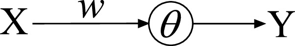

  

  TLU for questions 1 and 2

  Table 6.3 Truth table for question 1

  Hint: when X = 0, the weighted sum is w × 0 = 0. According to the model function Eq. 6.2, if 0 ≥ θ, the output Y will be 1. When X = 1, the weighted sum is w × 1 = w, and if w ≥ θ, the output Y will be 1. Therefore, the question can be rephrased as “Are there values of w and θ that can satisfy both 0 ≥ θ and w ≥ θ ?” If so, please give an example of the values for w and θ.

• 2. Can a TLU with a single input (Fig. 6.6) produce an output of 1 for X = 0 and an output of 0 for X = 1? In other words, can the truth table of a TLU be Table 6.4? If possible, please give an example of the weight w and threshold θ values that would achieve this.

  Table 6.4 Truth table for question 2

Hint: Similar to question 1, if there are values of w and θ that satisfy both conditions 0 ≥ θ and w < θ, it will be possible to output 1 and 0 for inputs 1 and 0, respectively. Consider if such values exist.

As shown in Figs. 6.5 and 6.6 and the above questions, the output of a neuron can vary for the same input if the weights and threshold values change. This ability to produce different outputs for the same input is a fundamental feature of neural network. This feature can be used to implement various functions.

Next, we provide an example of using a TLU to imitate the logic gate OR, one of the basic logic gates introduced in Sect. 1.7. This means we will demonstrate how to configure the weights and threshold of a TLU to produce the same results as the logic OR operation.

First, create a TLU with two inputs as shown in Fig. 6.7, because the logic gate OR has two inputs.

Fig. 6.7

A TLU with the same number of inputs as logic gate OR

Second, set the weights w₁, w₂, and threshold θ of the TLU to match the output of logic gate OR. The value-setting process includes three steps.

Step 1: create the truth table for the inputs and the correct outputs of the logic OR operation, as presented in Table 6.5. In this table, the inputs are A and B, and the output is T. When at least one input is one, the output will be one. Only when both inputs are zero will the output be zero.

Table 6.5 Truth table of the logic OR operation

Step 2: create a constraint for each of the four input patterns. For the input pattern A = 0 and B = 0, the weighted sum of inputs is w₁ × 0 + w₂ × 0. According to the model function Eq. 6.2, if this sum is less than θ, the output will be 0, matching the correct output (T column in Table 6.5). Therefore, the constraint is w₁ × 0 + w₂ × 0 < θ. In other words, we need to set the values of w₁, w₂, and θ to satisfy w₁ × 0 + w₂ × 1 < θ so that the TLU's output aligns with the logic OR output for this input pattern.

Similarly, for the input pattern A = 0 and B = 1, the weighted sum of inputs is w₁ × 0 + w₂ × 1. According to the model function, if this sum is greater than or equal to θ, the output will be 1, matching the correct output. Therefore, the constraint is w₁ × 0 + w₂ × 1 ≥ θ. In other words, we need to set the values of w₁, w₂, and θ to satisfy w₁ × 0 + w₂ × 1 ≥ θ so that the TLU's output aligns with the logic OR output for this input pattern.

In summary, when the correct output is 0, the weighted sum should be less than θ, and when the correct output is 1, the weighted sum should be greater than or equal to θ. The resulting four constraints are shown in Eqs. 6.3–6.6. Equations 6.7–6.10 are the calculation results, such as w₁ × 0 + w₂ × 0 = 0 and w₁ × 0 + w₂ × 1 = w₂.

$$ w_{1} \times 0 + w_{2} \times 0 < \theta $$

(6.3)

$$ w_{1} \times 0 + w_{2} \times 1 \ge \theta $$

(6.4)

$$ w_{1} \times 1 + w_{2} \times 0 \ge \theta $$

(6.5)

$$ w_{1} \times 1 + w_{2} \times 1 \ge \theta $$

(6.6)

$$ 0 < \theta $$

(6.7)

$$ w_{2} \ge \theta $$

(6.8)

$$ w_{1} \ge \theta $$

(6.9)

$$ w_{1} + w_{2} \ge \theta $$

(6.10)

Step 3: determine the values for w_i and θ that satisfy all the constraints. Since both w_i and θ are real numbers, numerous combinations can satisfy the four constraints. For example, w₁ = 2, w₂ = 2, θ = 1; w₁ = 2.4, w₂ = 1.7, θ = 0.6; and w₁ = 15.7, w₂ = 159, θ = 0.02.

After setting values for the weights and threshold, it is recommended to verify the TLU's actual output. For example, for a TLU with w₁ = 2, w₂ = 2, and θ = 1 (as shown in Fig. 6.8), you can calculate its actual output using Eqs. 6.11–6.14. When A = 0 and B = 0, the weighted sum of inputs is 0 × 2 + 0 × 2 = 0, which is less than the threshold 1, resulting in an output of 0. If all four actual outputs match the values in the T (target) column in Table 6.5, it is confirmed that the weights and threshold have been set correctly.

Fig. 6.8

A TLU with w₁ = 2, w₂ = 2, and θ = 1

$$ A = 0, B = 0 \to 0 \times 2 + 0 \times 2 = 0 < 1 \to Y = 0 $$

(6.11)

$$ A = 0, B = 1 \to 0 \times 2 + 1 \times 2 = 2 \ge 1 \to Y = 1 $$

(6.12)

$$ A = 1, B = 0 \to 1 \times 2 + 0 \times 2 = 2 \ge 1 \to Y = 1 $$

(6.13)

$$ A = 1, B = 1 \to 1 \times 2 + 1 \times 2 = 4 \ge 1 \to Y = 1 $$

(6.14)

Besides the logic OR operation, a single TLU can be employed to implement various logic operations, including the logic AND and combinations of logic circuits. Several examples will be given in the exercises.

6.3.3 Learning of TLU

The purpose of neural network learning is to enable a computer to automatically set the weights and thresholds for each neuron. For a TLU, the values to be set are w₁ to w_n and θ. During TLU learning, the input vector is (x₁, x₂,…, x_n), the correct output is t (target), and the actual output is y. If y ≠ t, the weight vector (w₁, w₂,…, w_n) and θ will be updated as follows [4].

$$ \forall i \in \{ 1,\,{\kern 1pt} ...,{\kern 1pt} \,n\} :\left\{ \begin{gathered} \theta^{(new)} = \theta^{(old)} + \Delta \theta ,\quad \Delta \theta = - \eta (t - y) \hfill \\ w_{i}^{(new)} = w_{i}^{(old)} + \Delta w_{i} ,\;\;\Delta w_{i} = \;\;\eta (t - y)x_{i} \hfill \\ \end{gathered} \right. $$

(6.15)

If the actual output y differs from the correct output t, Δθ will be calculated as the difference between y and t multiplied by a learning coefficient η. The new θ value is obtained by adding Δθ to the old θ value. Similarly, let Δw_i = η(t − y)x_i, the new w_i value is obtained by adding Δw_i to the old w_i value. These updates to θ and w_i will continue until y = t.

The learning coefficient η is in the range of (0, 1). When η approaches 0, the updates have smaller magnitudes, resulting in slower learning. Conversely, as η approaches 1, the updates become larger, potentially leading to faster learning. However, it is essential to note that increasing η indiscriminately does not necessarily accelerate learning. This is because overly large updates may hinder convergence of y toward the target t, especially when dealing with complex functions.

To illustrate this, consider the case where y is represented by a curve depicted in Fig. 6.9, and t is its lowest point. If the learning coefficient is set too high, the model may skip over many values during each iteration, making it challenging to reach t accurately. Therefore, selecting an appropriate value for η is crucial and should strike a balance between rapid learning and convergence to the desired output.

Fig. 6.9

An example of radical updates of y

• Questions

• 3. Which type of learning does the learning of a TLU belong to?

  • A. Supervised learning

  • B. Unsupervised learning

Hint: consider if the learning of a TLU needs the correct output or not.

The learning process of a TLU will update the weights (w₁, w₂,…, w_n) and threshold θ until the actual output y becomes the same as the correct output t. It is important to note that not all problems can be effectively solved using a single TLU. For example, in cases where there are no combinations of weights w_i and threshold θ values that can satisfy all the constraints, such as those illustrated in Eqs. 6.16–6.19, the TLU's learning process may never converge to a solution.

$$ 0 < \theta $$

(6.16)

$$ w_{2} \ge \theta $$

(6.17)

$$ w_{1} \ge \theta $$

(6.18)

$$ w_{1} + w_{2} < \theta $$

(6.19)

To address such problems, it becomes necessary to use a neural network with multiple neurons, and even hidden layers. In the upcoming section, we will provide a brief introduction to deep learning, which is a type of neural network characterized by its multilayered architecture.

6.3.4 Deep Learning

Deep learning is a problem-solving approach that uses large-scale hierarchical neural networks with multiple hidden layers.

Figure 6.10 illustrates the architecture of a deep learning neural network. A distinguishing characteristic of deep learning is that it is performed on neural networks with multiple (more than one) hidden layers. In other words, neural networks with zero (e.g. a TLU) or one hidden layer are commonly referred to as shallow networks rather than deep learning networks. Deep learning neural networks, as opposed to those with fewer hidden layers, exhibit superior capabilities in achieving higher accuracy in tasks like image and pattern recognition.

Fig. 6.10

Structure of a deep learning neural network

Deep learning offers several advantages, primarily stemming from its ability to handle complex data processing tasks when a sufficient amount of training data is available. With an ample dataset for training, a well-trained neural network can tackle tasks that are often too intricate for traditional machine learning algorithms. Furthermore, the accuracy of the trained neural network tends to increase proportionally with the quantity of training data.

On the downside, deep learning has its limitations. When the amount of training data is insufficient or when access to high-performance computing resources is lacking, deep learning may struggle to achieve high performance or become infeasible.

The most commonly used deep learning neural networks are Convolutional Neural Networks (CNNs) and Recurrent Neural Networks (RNNs).

CNNs are forward-propagating neural networks that excel at extracting local information and exhibiting location universality. Two-dimensional CNNs share structural similarities with neurons in the human visual cortex, which makes them particularly adept at pattern recognition. Figure 6.11 illustrates the architecture of a CNN used for image recognition.

Fig. 6.11

Structure of a CNN used for image recognition

The left part of a CNN, known as the feature extraction component, takes input images of various sizes and extracts features from them. This is performed using filters (also known as kernels) that are smaller than the input image. The filters act like windows, examining the image part by part as they traverse over the image (as shown in Fig. 6.12). On the right side, the classification component uses the extracted features to make predictions or determine the content of the image, outputting the final result. If you are interested in delving deeper into image recognition using CNNs, please refer to the reference [5].

Fig. 6.12

A filter moving over an image

RNNs are bidirectional neural networks that incorporate a recursive structure in its middle layers, where some of the outputs are used as inputs, as illustrated in Fig. 6.13. RNNs are well-suited for managing variable-length data, including audio and video, and they excel in tasks such as speech recognition, video recognition, and natural language processing.

Fig. 6.13

Bidirectional propagation in an RNN

Exercises

• 1. Use a TLU to implement the logic calculation X₁ AND X₂ AND X₃.

• Guidance

Figure 6.14 illustrates the TLU for this problem. You need to specify the values for w₁, w₂, w₃, and θ.

Fig. 6.14

A TLU with three inputs

First, create the truth table for the logic operation X₁ AND X₂ AND X₃. The truth table for the logic AND operation was previously provided and explained in Chap. 1. In case you need a refresher, please review it.

Table 6.6 is an example of a truth table with three inputs, X₁, X₂, and X₃. Each input has a value of either 0 or 1, resulting in a total of 2³ = 8 possible combinations. Please fill in the empty cells with the appropriate values.

Table 6.6 Truth table to complete for exercise problem 1

Once you have completed the truth table, proceed to derive a constraint based on the information in each row, following the examples provided in Sect. 6.3.2. Finally, set the values of w₁, w₂, w₃, and θ to ensure that all the eight constraints are satisfied.

• 2. Use a TLU to produce the output of the circuit shown in Fig. 6.15.

  Fig. 6.15

  

  Circuit for exercise problem 2

  • Guidance

  Similar to problem 1, start by creating the truth table for the circuit. This table should have two inputs, A and B, and one output. Since both A and B can be either 0 or 1, the table will consist of 2² = 4 rows.

  After completing the truth table, create a constraint based on the information in each row. Finally, set the values of the weights and threshold in such a way that all the four constraints are satisfied.

  If you need a visual representation of the TLU for this circuit, refer to Fig. 6.16. It depicts a TLU with inputs A and B, and only one neuron is enough. You should specify the values of w₁, w₂, and θ. Since a single neuron can produce the output for this circuit, there is no need to create additional neurons.

  Fig. 6.16

  

  A TLU for exercise problem 2

• 3. According to the content of this textbook, what is the relation between the three fields: artificial intelligence (AI), machine learning (ML), and neural network (NN)?

• Guidance

If we use three circles to represent the three fields, as shown in Fig. 6.17, then Fig. 6.18 indicates partial overlap between two fields, and Fig. 6.19 indicates one field entirely encompassing another. You can illustrate the relation between the three fields using such visual expressions.

Fig. 6.17

Diagram for exercise problem 3

Fig. 6.18

Expression of partial overlap between two fields

Fig. 6.19

Expression of one field encompassing another

• *4. Use a TLU to implement the logic operation X₁ AND (X₂ OR X₃).

• *5. Please explain why a TLU cannot produce the output shown in Table 6.7.

  Table 6.7 Truth table for exercise problem 5

References

Kruse R, Borgelt C, Braune C, Mostaghim S (2016) Introduction to neural networks. In: Computational intelligence. Texts in computer science. Springer, London. https://doi.org/10.1007/978-1-4471-7296-3_2
Orr G, Schraudolph N, Cummins F (1999) Lecture notes of neural networks. https://willamette.edu/~gorr/classes/cs449/intro.html
Blais A, Mertz D (2001) An introduction to neural networks—pattern learning with back propagation algorithm. Gnosis Software, Inc. https://www.sci.brooklyn.cuny.edu/~sklar/teaching/s06/ai/papers/nn-intro.pdf
Stergiou C, Siganos D (2011) Neural networks. https://wiki.eecs.yorku.ca/course_archive/2011-12/F/4403/_media/report.pdf
Ujjwalkarn (2016) An intuitive explanation of convolutional neural networks. https://ujjwalkarn.me/2016/08/11/intuitive-explanation-convnets/
Author information
Authors and Affiliations
Corresponding author
Rights and permissions
Copyright information
© 2024 The Author(s), under exclusive license to Springer Nature Singapore Pte Ltd.
About this chapter
Cite this chapter
Weng, W. (2024). Artificial Intelligence—Machine Learning. In: A Beginner’s Guide to Informatics and Artificial Intelligence. Springer, Singapore. https://doi.org/10.1007/978-981-97-1477-3_6
Download citation
DOI: https://doi.org/10.1007/978-981-97-1477-3_6
Published:
Publisher Name: Springer, Singapore
Print ISBN: 978-981-97-1476-6
Online ISBN: 978-981-97-1477-3
eBook Packages: Computer ScienceComputer Science (R0)