
Abstract
This chapter identified the variation and determinants of rice yield measured by the smart combine harvester, from among different rice yields within large-scale farms. Apart from to the paddy yield with 15% moisture, we studied the variations in the concerning ratios for unsorted and sorted brown rice as well. The sample included 351 fields from a farm corporation scaled over 113 hectares, located in the Kanto region of Japan. The candidate determinants were the field area and condition, nitrogen amount, time of transplanting or seeding, stage-specific growth indicators of chlorophyll content, number of panicles, plant height, and leaf plate value. In addition, soil properties, average temperature, and solar radiation were incorporated. Meanwhile, the varieties, cultivation practices, and soil types were adopted as dummy variables. The empirical analysis was conducted using multivariate linear regression, with logarithmic transformations of the continuous variables. The result indicated that panicle numbers in the full-heading stage and transplanting or sowing time were the most important continuous determinant, following by nitrogen amount, humus content, and so forth. Within the significant discrete determinants, Akidawara and Milky queen were found to be the productive and unproductive varieties, respectively, while the well-drained direct sowing was found to negatively affecting yield.
Access provided by Autonomous University of Puebla. Download chapter PDF
This chapter identified the variation and determinants of rice yield measured by the smart combine harvester, from among different rice yields within large-scale farms. Apart from to the paddy yield with 15% moisture, we studied the variations in the concerning ratios for unsorted and sorted brown rice as well. The sample included 351 fields from a farm corporation scaled over 113 hectares, located in the Kanto region of Japan. The candidate determinants were the field area and condition, nitrogen amount, time of transplanting or seeding, stage-specific growth indicators of chlorophyll content, number of panicles, plant height, and leaf plate value. In addition, soil properties, average temperature, and solar radiation were incorporated. Meanwhile, the varieties, cultivation practices, and soil types were adopted as dummy variables. The empirical analysis was conducted using multivariate linear regression, with logarithmic transformations of the continuous variables. The result indicated that panicle numbers in the full-heading stage and transplanting or sowing time were the most important continuous determinant, following by nitrogen amount, humus content, and so forth. Within the significant discrete determinants, Akidawara and Milky queen were found to be the productive and unproductive varieties, respectively, while the well-drained direct sowing was found to negatively affecting yield.
1 Introduction
Since coming back to power in 2012, the government has been pushing forward policies on proactive agriculture, forestry, and fisheries to increase the efficiency and competitiveness within these sectors in Japan. In agriculture, it is essential to reduce production costs and improve yields, through fiscal subsides for adopting efficient technologies, equipment, managerial models, among the others. To increase rice yield and reduce average production costs, the government declared that by 2018, the acreage reduction of rice adopted since the early 1970s will be abolished, to expand efficient production and exports along with improved international competitiveness (Nikkei 2013).
As the staple crop in Japan, rice accounted for the largest proportion in the gross agricultural output at 21.03% in 2013 (MAFF 2014a). After the post-war high economic growth, the extensive adoption of a western diet changed Japanese food consumption habits with increasing amounts animal products, such as meat, dairy products, eggs, oils, and fats. Together with the increasing share of the elderly and a decreasing population in general, the average annual consumption of sorted brown rice decreased from 111.7 kg per capita in 1965 to 55.2 kg per capita in 2014 (MAFF 2014b). Simultaneously, rice production also decreased and contributed to a reduction in agricultural growth to a large extent (Ohizumi 2014).
In Japan, rice yield is measured by the sorted brown rice grains with a thickness of no less than usually 1.70 mm. In 2014, the yield of sorted brown rice was 8.43 million metric tons, a decrease of 40.27% from 11.83 million metric tons in 1985. During the same period, the planted area of paddy decreased by 45.58%, from 2.29 million hectares to 1.57 million hectares. Since 2000, the average yield of sorted brown rice has been stagnant at approximately 5300–5400 kg per hectare. In 2014, the average yield of sorted brown rice was 5360 kg per hectare (E-Stat 2015), while in the US it was 7263 kg per hectare (USDA 2014). Paddy production in Japan is plagued with high costs. In 2014, the average production costs of sorted brown rice in Japan was 256.9 JPY per kilogram (MAFF 2016), much higher than that of the US, which was a mere 35 JPY per kilogram on average (USDA 2014). Note that, unlike Japan, rice yield in many other countries like the US, China, and Korea is measured by paddy weight—the raw rice grain without threshing the hull. Thus, for a better comparison, the above rice yield of the US was converted from paddy to sorted brown rice, using the ratio 1:0.8 (MAFF 2014d; Yaguchi 2012). As aforementioned in chapter “Smart Rice Farming, Managerial Model and Empirical Analysis”, the Japan Revitalization Strategy of 2014 aims to cut the costs of paddy production by 40% in the next 10 years (PMJHC 2014).
In the last few decades, agricultural production corporations have had a dramatic growth, from 2,740 in 1970 to 14,333 in 2014 (MAFF 2014c) and have become significant paddy producers. The major reasons for this growth are that unlike family management, agricultural production corporations possess larger arable lands and stronger managerial abilities, easier access to credit, diversified business development, better welfare, and sufficient human resources. Nevertheless, such large-scale farms usually have scattered fields, with different scales, soil properties, altitudes, humidity levels, daylight hours, and so on (JSAI 2014, p. 128). At the same time, to deal with the problems related to agriculture, food, and environment, GAP has been adopted widely in Japan. With respect to paddy production, GAP can improve people’s working and consuming conditions, provide environmental protection through appropriate application of agrochemicals, address the concerns over biodiversity, and ensure food safety that is free of contamination and nutritionally balanced (Li et al. 2014). In this circumstance, to increase the yield with saved costs of paddy production subject to GAP, ICT has been adopted and promoted, to process the enormous amount of information in sectors of innovational cultivation, production and managerial technologies (Nanseki 2015; JSAI 2014).
This book incorporated the research findings of “NoshoNavi1000”, series projects funded by the Japanese Ministry of Agriculture, Forestry and Fisheries (MAFF). Represented by Kyushu University, the project consortium includes four agricultural production corporations with 1000 paddy fields scaled over 330 hectares in total, two technology companies, five research institutes, and two universities (Nanseki 2015). It aimed to develop and demonstrate smart paddy agriculture models, implemented by agricultural production corporations, with the integration of ICT agricultural machinery, field sensors, visualization farming, and skill-transferring system. In this chapter, we investigated the variation in and determinants of rice yield, from among 351 fields at different planting stages, from a large-scale farm in Ibaraki Prefecture, Kanto Region, Japan. Unlike most previous studies that used experimental data, we used actual yield data measured by the smart combine harvester in the fields of a large-scale farm, with the cooperation of farm managers and field-work practitioners.
2 Materials and Methods
2.1 Yield Measurement and Estimation
According to the Japan’s standards of brown rice inspection (MAFF 2014e), the paddy yield used in the following analyses was converted using 15% of moisture content. The paddy before the conversion is called raw paddy, the weight and moisture content of which were monitored directly by the smart combine harvester equipped with GNSS (Isemura et al. 2015), and compared against the estimated weight of brown rice by sampling. Table 1 shows the calculation of rice yield for all 351 fields. Incidentally, rice yield is determined by four factors: panicle number, spikelet number per panicle, ratio of filled grains, and grain weight (CSSJ 2002).
In Japan, rice yield, as mentioned earlier, refers to the weight of sorted brown grains, while it is measured by weight of paddy grains in other countries. The difference is due to a complex process of measuring rice yield, which incorporates different concepts and ratios. Following the process shown in Fig. 7 of chapter “Smart Rice Farming, Managerial Model and Empirical Analysis”, we estimated paddy yield with 15% moisture, using the data of raw paddy and average moisture, measured by the smart combine harvester. Then, 2 kg of paddy from each field was sampled and hulled, based on which the weight of the brown rice was measured. The ratio of brown rice and, hence, the yield of unsorted brown rice were estimated in succession for each paddy field. At the same time, the hulled samples were sent to the laboratory in Kyushu University, where using another sample of 0.6 kg for each field, the brown rice grains thicker than 1.85 mm were sorted out through a grain-sorting machine. Finally, the yield of the sorted brown rice was estimated by multiplying the weight of brown rice with the ratio of sorted grains. For each field, the calculation of rice yield and summary statistics of concerning indices are shown in Table 1.
2.2 Explanatory Variables
To summarize the production and present the candidate yield determinants in the sampled fields, we built an indicator system of 48 continuous variables, from the perspective of field area and condition, nitrogen amount, and time of transplanting or seeding for the stage-based growth indicators. In addition, soil properties, average temperature, and solar radiation were incorporated to show the impact of natural conditions. The summary statistics are shown in Table 2.
-
(1)
Field property. There were significant variations among the paddy fields as revealed by the coefficient of variance, from 200 to 21148 m2 with an average of 3238 m2. The scores for the fields were evaluated by farm managers, considering the differences in height, water depth, water leakage, former crop, amount of inlet water, soil fertility, illumination, and herbicide application.
-
(2)
Production management. The proxy variable of transplanting date was converted by encoding April 14 as 1 and June 22 as 70 for all 351 fields. The nitrogen amounts measured were average weights calculated according to the amount and corresponding nitrogen content, including compost, compound chemical fertilizer, ammonium sulfate, and urea fertilizers.
-
(3)
Stage-specific growth indices. The different growth stages included panicle-forming, full-heading, 10 days following full-heading, and maturity. The growth indicators included the chlorophyll meter value of the SPAD, number of stems or panicles per hill, plant height, and individual and community LPV by the stage of panicle growth for the forming, heading, 10 days following full-heading, and maturity stages, as well as panicle length for only the maturity stage.
-
(4)
Temperature and solar radiation. We adopted precision devices to collect continuous data of temperature and solar radiation. The data shown in Table 2 was the average of 20 days following heading, as this span of time is vital for starch accumulation (Asaoka et al. 1985).
-
(5)
Soil property analysis. There were five aspects of soil properties considered: (1) fertility and texture including pH, EC, CEC, humus, and phosphate absorption coefficient; (2) saturation, constitution, and exchangeable amount of the base, by potassium, lime and magnesia content; (3) inorganic nitrogen in the form of ammonium and nitrate; (4) effective phosphoric and silicic acid; (5) amount of other elements, such as manganese, free iron oxide, soluble zinc, and copper.
We included the rice variety and cultivation regime to analyze the determinants of rice yield, like previous studies, including Nishiura and Wada (2012), Muazu et al. (2014), Ju et al. (2015). Soil properties can affect rice growth and yield in terms of nutrition content, water drainage and conservation, and aeration (CSSJ 2002). Therefore, we investigated the soil types of the sampled fields by referring to the Soil Information Navigation System of Japan (NIAES 2015). A dummy variable named soil type was formulated, with the binary values of gray lowland soil and peat soil. The summary statistics of these variables were provided in the following section.
2.3 Statistical Analysis
The impact of the independent variables, including the discrete and continuous variables, on the yield of sorted brown rice was analyzed using multivariate regression. The values of yield and the continuous variables were natural logarithmic transformations to enable an easier interpretation of the regression coefficients in terms of elasticity (Gujarati 2015). All the analyses were performed using SPSS 23.0 for Windows, and the Backward procedure was used to select the significant determinants of the ultimate model.
2.4 Variation in the Yields and Ratios
-
(1)
Correlation and variation
As shown in Table 1, the coefficients of variation (CVs) of average yield per hectare, including those of the paddy with 15% moisture, unsorted brown rice, and sorted brown rice, vary from 12 to 13%. In contrast, the ratio CVs of both the unsorted brown rice against paddy and the unsorted brown rice over sorted brown rice, were around 3%. Thus, there was greater fluctuation in the yields than the ratios. With respect to the correlation coefficients, the yield of sorted brown rice is significantly correlated with the other four indicators shown in Table 3. Among them, the coefficients of the two yields were greater than 0.95, much higher than those of the two ratios. This indicated that when comparing ratios, the yield of sorted brown rice is more linearly related to the yield of paddy and unsorted brown rice. Figure 1 plots the yield of the sorted brown rice and other yields and ratios, and the yields are scattered close to the estimated regression line, related to the yield of sorted brown rice.

Sorted brown rice yield and other yields and ratios of the 351 paddy fields of farm Y. a Sorted brown rice (kg/ha). b Sorted brown rice (kg/ha). c Sorted brown rice (kg/ha). d Sorted brown rice (kg/ha)
-
(2)
Variation among rice varieties
The variety of Akidawara had the highest value of both the paddy yield converted by 15% moisture (7303 kg per hectare) and ratio of the unsorted brown rice in the paddy (81%). Consequently, its yield of unsorted brown rice was the highest valued at 5934 kg per hectare. Simultaneously, Akidawara yielded the highest amount of sorted brown rice with 5426 kg per hectare, despite the lowest ratio of sorted brown rice against unsorted brown rice, which was merely 91%. It was then followed by the varieties of Akitakomachi, Ichibanboshi, Koshihikari, and Yumehitachi. While both are relatively low-yielding varieties, Mangetumochi had a higher yield of both paddy and unsorted brown rice than Milky queen. The former also yielded more sorted brown rice per hectare than the latter, thanks to a higher ratio of sorted brown rice to the unsorted brown rice (Fig. 2).

Rice yields and ratios among rice varieties in 351 fields of farm Y. a Panicles per hill in full-heading stage. b Date of transplanting/sowing (day). c Lime/magnesia. d Nitrogen from fertilizers per ha (kg). e Community LPV in panicle-forming stage f Humus (%). g Exchangeable potassium (mg/100 g). h Exchangeable manganese (%)
-
(3)
Variation among cultivation regimes or practices
The conventional transplant had the highest yield per hectare, measured in forms of both paddy (7053 kg) and sorted brown rice (5105 kg). This was followed by the yields of submerged direct sowing, at 6940 kg per hectare and 5057 kg per hectare, respectively. Submerged direct sowing yielded the highest amount of unsorted brown rice, at 5619 kg per hectare, with the highest ratio of 81% of unsorted brown rice to paddy. Well-drained direct sowing had the highest ratio of 97% sorted brown rice within the unsorted grains, while its average yield of 4846 kg of sorted brown rice per hectare had the third highest rank, due to the lowest paddy yield (Fig. 3).

Rice yields and ratios among cultivation regimes
-
(4)
Variation among soil types
There were some discrepancies between the two soil types, with respect to all the yields and ratios. In general, rice planted in the gray lowland soil yields more than the peat soil, while the average ratios of the latter were higher than the former. In the fields with gray lowland soil, the yields per hectare of paddy, unsorted rice, and sorted brown rice were 7069 kg, 5464 kg, and 5030 kg, which is 2.6, 1.6 and 1.2% higher than that of peat soil, respectively. At the same time, gray lowland soil gives 77.5% of unsorted brown rice in paddy and 92.2% of sorted brown rice in the unsorted ones, on average. Both ratios were lower than that of the fields in peat soil, although the differences were no more than 0.5% (Fig. 4).

Rice yields and ratios among soil types
3 Result and Discussion
As mentioned above, rice yield in Japan is mainly measured by the weight of sorted brown grain, which is causally related to the milled rice sold in the market. For each continuous variable, we presented the Pearson’s correlation coefficient and its significance with sorted brown rice yield in Table 3. These coefficients measured the linear association between each determinant and the yield, showing how strongly the two variables are linearly related and can be used as a reference in identifying the determinants of some variables. However, the correlation coefficient may lead to illusory results as it shows only a bilateral relationship, without considering the influence of other variables. Therefore, to identify the yield determinants of sorted brown rice, we need to conduct multivariate regression analysis. In this case, we can get significant models and determinants and partial correlation coefficients, which show the pure impact when other variables are held constant (Gujarati and Porter 2010). To amplify the relationships among yield and the determinants, logarithmic transformation was adopted for the continuous variables.
3.1 Results of the Multivariate Regression
In the initial multivariate regression model, the independent variables included all the continuous and discrete variables shown in Table 2. For each discrete variable, a dummy variable was formulated taking the value of 1 or 0 to indicate the presence or absence of a categorical effect. According to the result of the final model, 9 continuous and 3 discrete variables were included in the final model (Table 4). The adjusted R2 value denoted that 37.5% of the variation in the independent variable can be explained by 12 significant independent variables for this sample of 334 paddy fields. The significant F and t values showed that, both the model and each dependent variable made a difference in identifying the variation. The variance inflation factors (VIF) of all the dependent variables were less than 10; hence, eliminating the probability of collinearity. In the regression standardized residual plot shown in Fig. 5, the expected cumulated probability increases closely as the observed cumulated probability increases. This indicated that there is no heteroscedasticity in the final model (Carter et al. 2012).

Plot of regression standardized residual
In Table 4, column B contains the unstandardized estimated regression coefficients. For each continuous variable (Xi), the coefficient is the elasticity of yield with respect to Xi. For instance, the positive coefficient of X1 and the negative coefficient of X2 implied that yield can be increased by either more panicles per hill in the full-heading stage or earlier transplanting or sowing. For a certain level, a 1% increase in panicle number can increase the yield by 0.196%, while a 1% decrease in the transforming or sowing date value can increase the yield by 0.053%, holding other variables constant. For a more precise calculation, the estimated yield increased by 1.010.196−1 = 0.195% and 1.01−0.053−1 = −0.053%, respectively (Wooldridge 2013). Similarly, for the other significant determinants, a 1% increase in the nitrogen amount, community LPV in panicle-forming stage, humus, field area, and exchangeable manganese were estimated to increase the yield by roughly 0.046, 0.065, 0.036, 0.014 and 0.014%, respectively. Meanwhile, a 1% decrease in the ratio of lime to magnesia and exchangeable potassium, ceteris paribus, would increase the yield by roughly 0.1 and 0.034%, respectively. Table 4 shows the yield changes due to a 1% increase in each Xi as well. For the dummy independent variable Di, coefficient B implies yield changes by eB−1 when Di switches from 0 to 1, keeping other explanatory variables constant (Wooldridge 2013). Thus, for the variety of Akidawara, the coefficient of 0.153 denoted a roughly 15.3% higher yield, while the exact increase is 16.537%. Similarly, the variety of Milky queen, and well-drained direct sowing showed roughly 20.1%, and 23.6% lower yield on average, respectively, holding other factors constant (Table 4).
Within the continuous variables, an unstandardized coefficient B was affected by the units of measurement. We calculated the standardized coefficient, the absolute values of which show the relative importance of the explanatory variables. For example, according to the data in column Std. B in Table 4, panicle number in full-heading stage was shown as the most effective continuous factor to affect the yield of sorted brown rice. The variables in Table 4 were presented in the ascending rank of absolute values of Std. B, grouped in continuous and discrete variables.
3.2 Discussion on Impact of the Continuous Determinants
-
(1)
In the full-heading stage, 40–50% of the stalks have finished sprouting panicles. This is an important stage to judge the growth for the whole year (Goto et al. 2000). Thereafter, the focus of cultivation management shifts from the growth of stem and leaves to panicle growth and grain filling. In this stage, more panicles help to increase the yield directly according to the determined rice yield. This was shown in Fig. 6a, where the yield of sorted brown rice is plotted to rise upward with larger panicle numbers.
Fig. 6 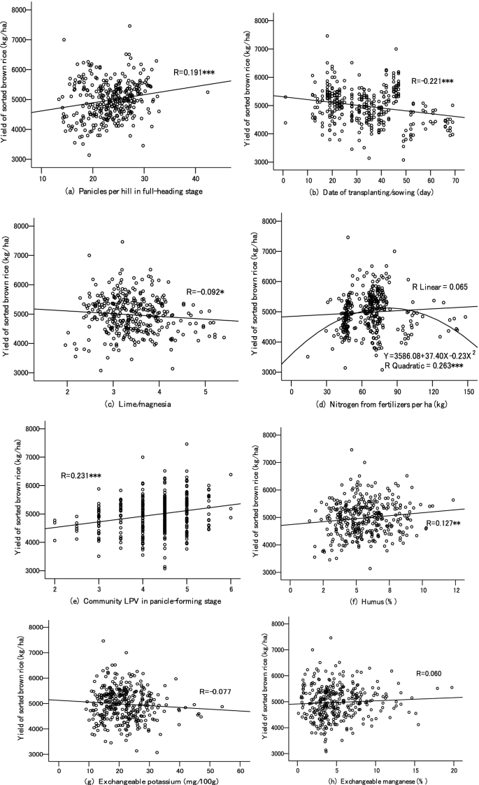
Scatter plots of sorted brown rice yield and determinants. a Panicles per hill in full-heading stage. b Date of transplanting/sowing (day). c Lime/magnesia. d Nitrogen from fertilizers per ha (kg). e Community LPV in panicle-forming stage. f Humus (%). g Exchangeable potassium (mg/100g). h Exchangeable manganese (%)
-
(2)
Relatively earlier transplanting or sowing benefits high yielding. Generally, earlier transplanting or sowing is followed by a longer vegetation period to accumulate more nutrients and benefit the growth in the later stages. In Li et al. (2015a), we identified that the growth duration gets shortened when the transplanting or sowing time is delayed. For example, the paddy transplanted during April 11–20 grew for 109 days before heading, while those transplanted or sowed during June 21–30 grew only for 58.5 days on average. The shortened vegetative growth usually results in reduced panicles, spikelets, and poor ripening ratio (NARO 2011). Figure 6b verified the trend of a downward yield when transplanting or sowing time is delayed.
-
(3)
Magnesia is the key ingredient of chlorophyll and, thus, indispensable for photosynthesis and for balancing the soil minerals. Nevertheless, its absorption efficiency is suppressed when the soil contains excessive lime. As shown in Fig. 6c, there was a positive correlation relationship, at the significance level of 0.01, between magnesia saturation and the yield of sorted brown rice.
-
(4)
As an essential element for paddy growth, nitrogen exists mainly in the forms of protein, especially Rubisco, which accounts for 20–30% of the total nitrogen amount (CSSJ 2002, p. 126). Generally, adequate nitrogen helps to increase the yield, as shown in Fig. 6d, by enhancing photosynthesis. More than 90% of crop biomass is derived from photosynthesis, and rice has been found to have a photosynthesis rate that is 10 times that of some evergreen trees (Makino 2011). Therefore, increasing nitrogen appropriately positively relates to yield, with no lodging or other negative consequences.
-
(5)
The panicle-forming stage is the young panicle grows to a length of 1–2 mm that is visible to the naked eye. This is an important stage in determining the optimum fertilizer amount and conducting panicle-length diagnosis. Further, the importance of preventing cold injury increases after this stage. To judge the nutrient content and decide the top-dressing amount, there is a quick way of reading the LPV, a higher grade of which indicates more nutrient content in the plant. Thus, this indicator positively related to yield, as plotted in Fig. 6e.
-
(6)
As a kind of polymeric compound transformed from organic matter, humus composes an important source of carbon, hydrogen, oxygen, nitrogen, sulfur, phosphorus, and other nutrient elements (Makino 1998). Humus can significantly improve the soil’s cation exchange capacity, hence contributing to store nutrient leached by rain or irrigation. On the other hand, humus can hold moisture up to 80–90% of its weight and strengthens the soil to withstand drought conditions. The biochemical structure enables humus to improve soil aeration and block toxic substances, excess nutrients, and excess acidity or alkalinity (Kono 1993). Thus, as shown in Fig. 6f, humus was positively correlated to the yield of sorted brown rice, significant at the 0.05 level.
-
(7)
The inverse impact of exchangeable potassium, as shown in Fig. 6g, revealed the reality of the last few years—surplus potassium is accumulated in the paddy fields of Japan, due to an over-use of fertilizers (Watanabe et al. 2015). Within the sampled paddy fields, the average potassium saturation amounted to 2.6%, higher than the maximum threshold of 2.5% of the paddy fields in Ibaraki Prefecture (MAFF 2008).
-
(8)
As an essential trace element for plant growth, manganese is involved in photosynthesis and the transformation of nitrogen, and it is active in the catalysis of many enzymes and redox processes. It can promote the synthesis of chlorophyll and the operation of carbohydrates. The deficiency of manganese in soil may lead to withered plants, dysplasia, and eventually, declined production. Thus, there was a positive relationship between the amount of exchangeable manganese and the yield of sorted brown rice, as shown in Fig. 6h.

Within this sample, 312 fields were less than 0.7 hectares in size, up to which positive correlation coefficients were observed for the yield of sorted brown rice and field area (Fig. 7). It can be interpreted that when fields are scaled less than 0.7 hectares, a larger area can usually increase yield through an enlarged sink size (i.e., spikelet number per unit land area). Meanwhile, the correlation coefficient of the field area and amount of nitrogen from fertilization was 0.46, significant at 0.01 level, indicating that a larger field facilitates application of fertilizer. Nevertheless, both factors indicated the existence of diminishing returns when inputs are increased over threshold values. As shown in Figs. 6d and 7, yield per hectare decreased in the fields more than 0.9 hectares in size, or when the nitrogen amount exceeds approximately 90 kg per hectare.

Correlation coefficients of field area and sorted brown rice yield
3.3 Discussion on the Impact of Discrete Determinants
As we have demonstrated in another study (Li et al. 2015a), rice variety was a significant factor that affects paddy yield in this sample. Akidawara is a new, lodging-resistant, and high-yielding variety and is suitable for cultivation in the Kanto Region. In this chapter, Akidawara yielded 7303 kg per hectare on average, the highest among the seven varieties observed. The average yield of the other six varieties was 6812 kg per hectare, 7.21% lower than that of Akidawara (Fig. 2). Further, Akidawara had, on average, the longest growth period of 80 days—from transplanting to heading—almost 10 days more than the other varieties. Thus, as analyzed above, it has an advantage of a prolonged vegetative growth with more panicles, spikelets, and increased ripening ratio, and so on. in contrast, Milky queen is a new rice variety bred in Koshihikari, with low amylose content in the endosperm. The Milky queen is not adapted to heavy chemical fertilizer use in paddy fields because it is susceptible to lodging after the heading stage and leaf- and panicle-blast diseases. In addition, Milky queen has low resistance to rice blast disease (Ise et al. 2001). Therefore, as shown in Fig. 2, the sorted brown rice yield of Milky queen was 3829 kg per hectare, the lowest among the seven varieties.
Direct sowing is one of the traditional cultivation regimes and it has significant savings in labor and energy inputs. However, due to unstable establishment, poor resistance to weed damage, and susceptibility to lodging, directly sowed rice yield is less than that of transplanted one, in general. In the well-drained direct sowing, its drawbacks are that sowing time is dependent on the weather, nutrient loss from cracked soil, and so on (CSSJ 2002, pp. 326–329). The survey data shows that the yield of paddy cultivated using well-drained direct sowing was the lowest, with the largest data dispersion denoted by CV, among the five cultivation regimes observed. In addition, it had the lowest number of panicles in the heading stage. Submerged direct sowing was used only to cultivate Akidawara, for which the average yield by submerged direct sowing was less than from the other cultivation regimes.
4 Conclusion
In the initial multivariate regression analysis, the candidate determinants included a variety of continuous variables of yield, field characteristics, transplanting time, nitrogen amount from fertilization, and growth data at different stages. In addition, three discrete variables were included for variety, cultivation regime, and soil type. The result of the multivariate regression analysis showed that, the panicle numbers in the heading stage and an earlier transplanting date are the most important determinants in increasing rice yield. The other significant determinants were: nitrogen amount, humus content, exchangeable manganese, and community LPV in the panicle-forming stage, ratio of lime to magnesia, and exchangeable potassium, all of which have a positive impact on the yield of sorted brown rice. Within the discrete determinants, the Akidawara and Milky queen were observed as the high-yield and low-yield varieties, respectively; while the well-drained direct sowing was shown as negatively affecting the yield of sorted brown rice. The regression coefficients indicated a positive impact of field area on yield, while the correlation coefficient and further analysis from the scatter plot show that extremely high values could lead to yield reduction.
We can use these empirical findings as a reference to increase yield in farm management. Nevertheless, paddy production in large-scale farms is a systematic procedure, subject to constraints of labor, funds, machinery, and so on. For instance, although earlier transplanting or sowing is shown to increase yield, it might be unrealistic or uneconomical to conduct transplanting or sowing in many fields simultaneously. Thus, optimal planning is necessary to conduct transplanting or sowing at different times while making full use of the limited machinery, labor, and funds (Chomei et al. 2015). Moreover, the amount of fertilizer and allocation of fields of different sizes must be optimized in future studies, considering the properties of different rice varieties. As analyzed above, the direct sowing was negatively related to a yield increase, but it promotes sustainable development. Hence, more rice varieties suitable for direct sowing should be bred and cultivated.
References
Asaoka, M., Okuno, K., Sugimoto, T., & Fuwa, H. (1985). Developmental changes in the structure of endosperm starch of rice (Oryza sativa L.). Agricultural and Biological Chemistry, 49, 1973–1978. https://doi.org/10.1271/bbb1961.49.1973.
Carter, R. H., William, E. G., & Guay, C. L. (2012). Principles of econometrics (4th international edition, p. 303). Hoboken, NJ: Wiley.
Chomei, Y., Nanseki, T., Aga, S., & Miyazumi, M. (2015). Relationship between the managerial goals, revenue, and costs in large-scale paddy farm: Optimization analysis considering the operational risks. In Proceeding of annual symposium of the Japanese Society of Agricultural Informatics (JSAI) (in Japanese).
CSSJ (Crop Science Society of Japan). (2002). Encyclopedia of crop science (pp. 126, 210, 326–329, 522). Tokyo: Asakura Publishing Co., Ltd. (in Japanese).
E-Stat. (2015). Statistics on the crops planted in 2014. http://www.e-stat.go.jp/SG1/estat/List.do?lid=000001129556 (in Japanese).
Goto, Y., Nitta, Y., & Nakamura, S. (2000). Crops I: Paddy cultivation (pp. 120, 137–142, 195, 210–211). Tokyo: Japan Agricultural Development and Extension Association (JADEA) (in Japanese).
Gujarati, D. N. (2015). Econometrics by example (2nd ed., pp. 44, 81, 136–138, 254). London: Palgrave.
Gujarati, D. N., & Porter, D. C. (2010). Essentials of econometrics (4th ed., p. 254). New York: McGraw-Hill.
Ise, K., Akama, Y., Horisue, N., Nakane, A., Yokoo, M., Ando, I., et al. (2001). Milky queen, a new high-quality rice cultivar with low amylose content in endosperm. Bulletin of NARO Institute of Crop Science (NICS), 2, 39–61. (in Japanese).
Isemura, H., Hisamoto, H., Yokota, S., Butta, T., Fukuhara, Y., Takasaki, K., et al. (2015). Field demonstration on the paddy yield measurement and operation video recording. In Proceeding of the annual symposium of the Japanese Society of Agricultural Informatics (JSAI) (in Japanese).
JSAI (Japanese Society of Agricultural Informatics). (2014). Smart agriculture: Innovation and sustainability in agriculture and rural areas (pp. 128–149). Tokyo: Agriculture & Forestry Statistics Press (in Japanese).
Ju, C., Buresh, R. J., Wang, Z., Zhang, H., Liu, L., Yang, J., et al. (2015). Root and shoot traits for rice varieties with higher grain yield and higher nitrogen use efficiency at lower nitrogen rates application. Field Crop Research, 175, 47–55.
Kono, E. (1993). Humus. Japanese Journal of Agricultural Engineering, 61(12), 56. (in Japanese).
Li, D., Nanseki, T., & Chomei, Y. (2014). Managerial models of smart paddy agriculture and the adoption of GAP in Japan. Proceeding of the 8th International symposium on the East Asian Environmental Problems (EAEP) (pp. 130–135). Fukuoka: Hanashoin Press.
Li, D., Nanseki, T., Matsue, Y., Chomei, Y., & Shuichi, Y. (2015a). Empirical analysis on determinants of paddy yield measured by smart combine: A case study of large-scale farm in the Kanto Region of Japan. In Proceedings of annual symposium of the Japanese Society of Agricultural Informatics (JSAI).
MAFF. (2008). Japan national criteria for promoting soil fertility. http://www.maff.go.jp/j/seisan/kankyo/hozen_type/h_dozyo/pdf/chi4.pdf (in Japanese).
MAFF. (2014a). Statistics on incomes from agricultural production. http://www.maff.go.jp/j/tokei/kouhyou/nougyou_sansyutu/ (in Japanese).
MAFF. (2014b). Statistics of food self-sufficiency. http://www.maff.go.jp/j/tokei/sihyo/data/02.html (in Japanese).
MAFF. (2014c). Data of agricultural production corporations. http://www.maff.go.jp/j/keiei/koukai/sannyu/pdf/seisan.pdf (in Japanese).
MAFF. (2014d). Present situation and countermeasures of rice production costs. https://jataff.jp/project/inasaku/koen/koen_h25_2.pdf (in Japanese).
MAFF. (2014e). Inspection standards of brown rice. http://www.maff.go.jp/j/seisan/syoryu/kensa/kome/k_kikaku/index.html (in Japanese).
MAFF. (2016). Statistics on agricultural production costs of Japan. http://www.maff.go.jp/j/tokei/sihyo/data/12-2.html (in Japanese).
Makino, A. (2011). Photosynthesis, grain yield, and nitrogen utilization in rice and wheat. Plant Physiology, 155, 125–129.
Makino, T. (1998). Humus and its function. Japanese Journal of Agricultural Engineering, 66(1), 82. (in Japanese).
Muazu, A., Yahya, A., Ishak, W. I. W., & Bejo, S. K. (2014). Yield prediction modeling using data envelopment analysis methodology for direct sowing, wetland paddy cultivation. Agriculture and Agricultural Science Proceedings, 2, 181–190.
Nanseki, T. (2015). ICT application in the research project of NoshoNavi1000. In Proceeding of annual symposium of the Japan Society of Agricultural Informatics (JSAI) (in Japanese).
NARO. (2011). Technical precautions upon the late transplanting rice. http://www.naro.affrc.go.jp/nics/webpage_contents/sinsai/banshoku/index.html (in Japanese).
NIAES (National Institute for Agro-Environmental Sciences). (2015). Soil Information Navigation System. https://soil-inventory.dc.affrc.go.jp/ (in Japanese).
Nikkei (Japan Economic News). (2013). The government decided to abolish the rice acreage reduction policy in 5 years. http://www.nikkei.com/article/DGXNASFS2600F_W3A121C1MM0000/ (in Japanese).
Nishiura, Y., & Wada, T. (2012). Rice cultivation by direct sowing into untilled dry paddy stubble: Panicle number and rice yield. EAEF, 5(2), 71–75.
Ohizumi, K. (2014). Analysis on the perspective agriculture of Japan (pp. 16–18). Tokyo: NHK Books (in Japanese).
PMJHC (Prime Minister of Japan and His Cabinet). (2014). Revitalization strategy: Japan’s challenge for the future. http://www.kantei.go.jp/jp/singi/keizaisaisei/pdf/honbunEN.pdf.
USDA. (2014). Current costs and returns of rice. http://www.ers.usda.gov/data-products/commodity-costs-and-returns.aspx.
Watanabe, Y., Sasaki, S., Sato, H., & Sato, M. (2015). Development of SSR marker sets for the identification of rice breeding and cultivars in Fukushima Prefecture. Tohoku Journal of Crop Science. 58, 21–22.
Wooldridge, J. M. (2013). Introductory econometrics: A modern approach (5th international edition, pp. 183, 224–225). Cengage Learning.
Yaguchi, K. (2012). Several issues on the Expanding scales of agricultural management and land integration: Approaching to the TPP. Issue Brief of Japan National Diet Library, 737, 1–12. (in Japanese).
Author information
Authors and Affiliations
Corresponding author
Editor information
Editors and Affiliations
Rights and permissions
Copyright information
© 2021 The Author(s), under exclusive license to Springer Nature Singapore Pte Ltd.
About this chapter

Cite this chapter
Li, D., Nanseki, T., Matsue, Y., Chomei, Y., Yokota, S. (2021). Variation in Rice Yields and Determinants Among Paddy Fields. In: Li, D., Nanseki, T. (eds) Empirical Analyses on Rice Yield Determinants of Smart Farming in Japan. Springer, Singapore. https://doi.org/10.1007/978-981-33-6256-7_2
Download citation
DOI: https://doi.org/10.1007/978-981-33-6256-7_2
Published:
Publisher Name: Springer, Singapore
Print ISBN: 978-981-33-6255-0
Online ISBN: 978-981-33-6256-7
eBook Packages: Economics and FinanceEconomics and Finance (R0)