Design and Development of Electric Powertrain for a Proposed Three-Wheel Personal Mobility Vehicle

Abstract

This paper presents the design and development of the powertrain for a three-wheeled electric vehicle having a tadpole configuration with rear wheel drive. This three-wheeler, aimed at personal mobility, is designed for a top speed of 50 kmph with a range of 20–25 km per charge fueled by highly efficient Lithium-ion batteries with a reduction ratio of 6.2:1 split into two stages and powered by a 6 kW electric motor. Tractive force simulations for the prescribed vehicle parameters were carried out using the QSS toolbox of MATLAB-Simulink by choosing the appropriate drive cycle post the drive cycle analysis. Motor Sizing and Battery Sizing procedures along with suitable reduction ratio ensured the perfect selection of motor and battery pack combination for the required performance parameters and efficient output of the system. Following sizing procedures, the various components of the drivetrain were checked for interference and finally integrated on the swing-arm of the vehicle post analysis of all the components involved.

1 Introduction

In the present scenario, transportation accounts for one-fourth of all carbon emissions. The transport sector is witnessing rapid growth and is expected to reach one-third of the overall carbon emissions. Although developing countries have the fastest growing fleets, the majority of them have no vehicle emissions standards, programs and incentives in place to promote zero emission vehicles. Introduction of electric vehicles especially three wheelers for congested city traffic serves to be an excellent alternative to combat the pollution caused by ICE vehicles. In order to achieve a cleaner transport sector, a combination of measures such as well-designed cities, increased usage of public transport and cleaner on-road fleets like electric vehicles have to be implemented. Of the above-suggested measures, the introduction of Electric Buses, Electric Light duty Vehicles and Electric Two and Three Wheelers offers a higher impact towards green mobility solutions. Thus, the first priority in moving towards electric mobility is by replacing the present conventional two and three wheelers with electric ones.

1.1 Electric Motor Versus IC Engine

The electric motor or an IC Engine are designed to convert one form of energy into useful mechanical work to propel a vehicle.

The IC Engine: An IC engine, by design, must rotate to generate torque. It must suck in air, compress it and remove it. This cannot be achieved at low RPM. A piston makes power only 25% of the time and it has to pay for the remainder of the strokes. So, it must rotate at a modest speed to generate ample power. ICEs convert linear motion from pistons into rotational motion and hence have to overcome a lot of internal friction. For this reason, ICE’s do not operate much below 700 RPM and do not establish any serious torque until at least 1000 RPM and max torque around 3500 RPM.

The Electric Motor: Electric motors, on the other hand, include just wires and magnets. When current is passed through the wire, it becomes a magnet, this pushes against another magnet and develops force. More the current supply, more the force. The greatest current usually runs at 0 RPM, as there's practically zero resistance in the wires. Compared to an ICE, they have very few components and very low internal friction. Electric motors can also operate at any speed from 0 RPM up to their maximum RPM. They have an almost constant torque profile from 0 RPM up to their highest rated power (Figs. 1 and 2).

Fig. 1

A typical IC engine performance curve

Fig. 2

A typical electric motor performance curve

1.2 Electric Powertrain

The powertrain of any vehicle includes the components which generate the required power and transmit the same to the wheels in order to propel the vehicle. In an electric powertrain, the source of the propulsive energy arises from an electric motor. The other major components in an electric powertrain include the battery pack, transmission system and controllers.

1.3 Challenges in City Mobility—Last Mile Connectivity

Last Mile connectivity often describes the means of transport which is responsible for getting people from various transportation hubs to their final destination. Environmentalists are facing a lot of challenges as people often revert back to conventional combustion vehicles. Electric vehicles, when used for this specific purpose, need not worry about the range, charging facilities etc. while providing pollution-free rides. Personalizing mobility by the introduction of electric two and three wheelers will help in achieving a greener last mile connectivity.

1.4 Three Wheelers

Three wheelers have two different orientations namely:

• Tadpole: This orientation consists of two wheels in the front and a single wheel in the rear.

• Delta: This orientation consists of two wheels in the rear and a single wheel in the front (Figs. 3 and 4).

  Fig. 3

  

  Delta and Tadpole configuration

  Fig. 4

  

  The steering wheels in Delta and Tadpole

Tadpole Design: The Tadpole design as mentioned above, has higher stability during hard braking, also the two wheels in the front provide greater support while taking sharp turns and handling lateral acceleration loads. This configuration has improved aerodynamics and it also facilitates the usage of small lightweight motors in the rear. Furthermore, the usage of a front wheel drive vehicle will increase the transversal stability and the rear wheel-driven tadpole design ensures the complete transfer of drive to surface. Hence, this configuration is more advantageous than Delta type and is subsequently used for the construction of this mobility vehicle.

2 Literature Review

Łebkowski [1], in his work on electric vehicles mentions that electric vehicles can substantially reduce the local emission of noxious gasses into the environment. He also mentions the decreased energy consumption and efficiency of electric vehicles during their operation. Choi and Jahns [3] have worked on a specialized design evaluation tool for electric machines intended for use in electric vehicles that seek to maximize the machine’s efficiency in the operating regions that most closely correspond to the vehicle’s driving schedules and influences of different designs on a production battery-electric vehicle based on different driving cycles for optimization of EV range are studied. Karamuk [4] has extended the study on operation modes of an electric vehicle on the torque-speed curve of an electric motor for different driving scenarios. He has conducted a survey to review the essential components of an electric powertrain and based on simulations in Matlab-Simulink for sizing of electric motors considering the vehicle performance. Balamurugan and Manoharan [5] have stressed on the selection of PMDC motor over a commercially available induction motor and suggested that the increased number of bushes would apparently improve the overall motor efficiency. Butler et al. [6] have mentioned that computer modelling and simulation, if done, lead to reduction in the expense and the length of design cycle of electric vehicles before the prototype construction begins. They have also carried out various simulations implementing drive cycles and compared the energy consumption between them. Andres et al. [7] suggested that the utilization of a reduction gearbox in an electric vehicle results in an improvement of overall energy consumption along with the required torque for a defined acceleration performance. The investigation also proved that the efficiency increase is achieved by selecting appropriate gear ratios thereby reducing machine losses and energy demands. Lee and Ahmed [9] mentioned during their work on development of electric powertrain that the battery package can be used as a rechargeable energy source. They also suggested the use of LiFePO4 as battery cells for a better life and compact packaging. Their experiments proved that properly designed battery packs provide the required energy to the motor successfully. Park et al. [11], mentioned in their work related to dynamics of EV that Integrated modelling considering both the mechanical and electrical systems is essential. They acknowledged that integrated modelling is necessary in order to assess ultimate kinetic and dynamic characteristics of an Electric Vehicle.

2.1 Problem Statement

One of the major causes for the constant degradation of the air quality especially in urban areas is the emissions from combustion vehicles. With the reference to the above-stated text along with the literature survey carried out, it is the need of the hour to find a replacement for the conventional IC engine run vehicles. With this as background, we came up with the idea of designing a pure electric powertrain for a three-wheel vehicle which would be used within city limits as a personal mobility vehicle aiming to solve the above stated challenges.

2.2 Vehicle Parameters

Since the Electric Powertrain is specifically designed for a vehicle which is targeting the urban transport sector, it aims to solve trivial problems like last mile connectivity and the most important being to cut down harmful emissions. With this as foundation we will have to design a Powertrain which meets the above standards while most of the parameters of the proposed vehicle will be defined only after a thorough investigation. The proposed vehicle parameters are as—Top Speed: 50 kmph; Acceleration: 2.2 m/s²; Max Gradient: 14°.

2.3 Methodology

The work is split into three phases consisting of literature survey, design and development and finally integration and optimization of the electric powertrain for improved performance. The initial phase of the literature survey involves the understanding of the electric powertrain and the challenges faced in the current scenario. In further stages, studies on different driving cycles are carried out. After the selection of a suitable driving cycle, motor and wheel selection is done, wherein the appropriate motor and wheel dimensions as per power requirements are chosen in coordination with the suspension and brakes team. Simulations are performed on the QSS Module of MATLAB-Simulink, to cross verify the different parameters for the considered vehicle performance. Post selection of motor and wheels, the required size of the battery and the reduction ratios are calculated. Battery sizing is also done on the QSS module of MATLAB-Simulink to cross verify the results after which the drive is selected. Post battery sizing and drive selection, final drive components are designed on SOLIDWORKS. Modal and structural analysis are performed on the designed components on ANSYS. The components are then assembled in SOLIDWORKS for efficient packaging.

3 Driving Cycle

Driving Cycle is a series of data points representing the speed of a vehicle with respect to time developed by various countries and organizations. There are two major types of driving cycles:

• Transient—Involves many changes that represent the continuous change in speed of a vehicle as seen in typical on-road vehicles.

• Modal—Represents protracted periods at constant speeds.

The transient kind of driving cycle is the most preferred kind as it gives us a continuous change in vehicle parameters with respect to time unlike the modal driving cycle, which gives changes in parameters only after a certain fixed time. Knowledge of driving cycles in various regions is important for comparative testing and vehicle design purposes. The various uses of driving cycles are:

• Analyze powertrain operation and resulting fuel consumption

• Variation of road gradients and it’s effect on performance parameters.

• Performance variation by considering various conditions like traffic density, environmental effects etc.

3.1 Available Driving Cycles

Most of the currently used driving cycles originated in Europe. Further, the United States, China and India have played a significant role in adding new driving cycles. Some of the commonly used driving cycles are NEDC—New European Drive Cycle, FTP—Federal Test Procedure and WLTC—Worldwide Harmonized Light vehicle Test Cycle.

The following observations are noted from the above-listed drive cycles:

• FTP—75 cycle does not take into consideration the road gradient and this scenario does not hold good for Indian roads.

• The New York City cycle was developed with the aim to represent driving in highly congested urban traffic, typical for a city with frequent stops and idling.

• The NEDC driving cycle was the most widely followed drive cycle in the automotive industry before the introduction of the WLTP cycle as it includes both urban and highway driving regimes.

• WLTP has been in use since September 2017 and is a global standard driving cycle as it has data from all major countries and all types of road conditions. WLTP Class 01 is used specifically for low-speed vehicles.

Based on the above study, it was decided that NYCC and WLTP Class 3–2 low were the most suitable cycles, which can be considered for the design of our proposed personal mobility vehicle.

The consolidated data collected from various standard driving cycles is mentioned in Table 1 (Fig. 5).

Table 1 Consolidated drive cycle data

Fig. 5

Image comparing WLTC Class 2 and 3 Cycle

4 Motor Sizing

Motor sizing refers to the process of selecting the correct motor for a given load. The sizing method enables the usage of the maximum machine speed to reduce the torque requirement on the electric machine which in turn minimizes its size, cost and power.

4.1 Procedure

The steps to determine the size of the motor suitable for our application is as follows:

• 1. Determine the traction forces of the vehicle, based on its performance requirements.

• 2. Select the speed and operating range of the motor required, through market research and survey.

• 3. Determine the required gear reduction ratio, based on the maximum required vehicle speed and the maximum motor speed.

• 4. Determine the maximum required torque to overcome the maximum traction force.

• 5. Determine the power required based on the maximum required torque, which is the required motor power.

4.2 Quasi-Static Simulation (QSS) Approach

QSS toolbox is a MATLAB-Simulink toolbox developed by the University of Zurich. It follows a backward simulation approach that is quasi-stationary simulation of Hybrid and Electrical powertrain mainly directed towards their correct sizing, optimization and energy flow in them. This tool consists of several blocks representing the main components of a powertrain like the engines, electrical motors, electrical storage devices, transmissions and other mechanical coupling equipment. The above-mentioned toolbox is implemented for the calculation of the tractive force required to overcome the various resistances that the vehicle is expected to encounter by the utilization of the vehicle model (Figs. 6 and 7).

Fig. 6

An overview of the QSS toolbox

Fig. 7

The vehicle model in QSS toolbox library

4.3 Vehicle Driving Forces

The major resistive forces experienced by a vehicle are rolling resistance of tires, aerodynamic drag, gradient and acceleration forces.

The above-mentioned forces on the car are given by the following mathematical equations:

• Rolling resistance,

  $${\text{F}}_{{{\text{roll}}}} = \mu_{r} * m * g$$

  (1)

• Aerodynamic drag,

  $${\text{F}}_{{{\text{aero}}}} = 0.5*\rho *C_{d} *A*v^{2}$$

  (2)

• Gradient force,

  $${\text{F}}_{{{\text{grade}}}} = m * g * \sin \alpha$$

  (3)

• Acceleration force,

  $${\text{F}}_{{{\text{Net}}}} = m * a$$

  (4)

• Traction force,

  $${{\text{F}}}_{{{\text{Trac}}}} {\text{ = F}}_{{{\text{Net}}}} {\text{ + F}}_{{{\text{grade}}}} {\text{ + F}}_{{{\text{aero}}}} {\text{ + F}}_{{\text{roll`}}}$$

  (5)

These forces add up to make the tractive force required by the vehicle to meet the desired performance parameters. The force from the vehicle powertrain should exceed the tractive force of the vehicle for the vehicle to move from rest.

A simulator model is then built in MATLAB-Simulink to determine the tractive force of the vehicle under different conditions. The model is as shown (Fig. 8).

Fig. 8

The various elements of the vehicle block

This model contains a vehicle block, which requires a ramp generator function for providing the time varying velocity input to the vehicle block and also requires scope and an XY—Plot for viewing the output in the required graphical format. The addition of the appropriate driving cycle block to the module is necessary for obtaining accurate values of the simulation. City-2 driving cycle was chosen for this iteration. The vehicle block requires various input parameters which are further explained.

4.4 Vehicle Parameters

• Considered Mass of the Vehicle – 270 kg (Driver and Pillion)

• Frontal Area of the Vehicle – 0.6 m²

• Drag coefficient – 0.5 [13]

• Rolling resistance coefficient – 0.02 [14]

• Mass increase due to Rotating inertia – 5%

• Top Speed to be achieved – 50 kmph/ 13.88 m/s

• Assumed gradients are - 3° (0.052 rad), 7° (0.122 rad) & 14° (0.244 rad)

Input parameters: Vehicle speed, Vehicle acceleration, Road inclination angle.

Output parameter: Traction force of the vehicle.

The vehicle performance requirements for different conditions are shown in Table 2.

Table 2 The results of the traction force iterations

After obtaining the traction forces (F_Trac) for different driving conditions, we move onto the subsequent steps, taking the highest possible value of traction force (F_Trac) for further calculations. The obtained values were validated by hand calculations using:

$${\text{F}}_{{\text{Trac}}} {\text{ = F}}_{{\text{Net}}} {\text{ + F}}_{{\text{Roll}}} {\text{ + F}}_{{\text{Aero}}}{ + } {{\text{F}}_{{\text{Grade}}}}$$

(6)

The values obtained were found to have a deviation of 3.8%, 0.37% and 0.14% respectively, hence validating our results.

4.5 Gear Reduction

If the electric machine is at its maximum speed when the vehicle runs at its top speed, the highest possible gear ratio is achieved. The highest gear ratio minimizes the required torque of the electric machine. As cost is roughly proportional to the torque of the machine, it is clear that using the highest possible gear ratio reduces the machine cost. The required gear ratio is calculated from the equation:

$${\text{Gear ratio, i }} = \frac{{\omega EM * r_{wheel} }}{{V_{vehicle} }}$$

(7)

The vehicle has a wheel radius of, ${r}_{wheel}$= 0.203 m and is required to travel at a speed of, ${V}_{vehicle}$ = 50 kmph at a motor speed of, ${\omega }_{EM}$ = 428.4 rad/s. Substituting these values in the above equation results in the gear ratio, i = 6.2.

4.6 Torque Requirements

The torque required from the motor is given by,

$$T_{EM} = \frac{{F_{Trac} * r_{wheel} }}{i}$$

(8)

We have already calculated the values of parameters required to calculate the torque. The vehicle experiences a traction force of, F_Trac = 848 N with a wheel radius of, ${r}_{wheel}$= 0.203 m and a gear reduction value of, i = 6.2.

Substituting these values in the above equation results in a torque value of, T_EM = 27.7 Nm, which is the maximum required torque from the electric motor.

4.7 Power Requirements

The power output required from the motor is given by:

$${\text{P}}_{{{\text{EM}}}} = \omega_{{{\text{EM}}}} *{\text{ T}}_{{{\text{EM}}}}$$

(9)

Torque required from the electric motor as per the previous calculation is, T_EM = 27.7 Nm at a motor speed of, ${\omega }_{EM}$ = 428.4 rad/s.

Substituting these values in the above equation results in a power output of, P_EM = 11.86 kW, which is the required power from the electric motor for the necessary vehicle performance.

4.8 Motor Availability

Based on the above calculations, an electric motor having a power rating of 11.86 kW and torque in the range of 27.7 Nm is to be used, if the vehicle is to reach the performance levels previously mentioned. A motor having the above specifications is not readily available in the University. So, a 6 kW motor with a peak power of 8.6 kW is used in this case. By using a lower power motor, we will be compromising our acceleration, against the desired value.

5 Reduction Ratio

When it comes to electric vehicles, multi-speed gearboxes are not necessary. As a single reduction ratio is sufficient for operation, the ratio must be chosen to support both acceleration and top speed. A very low ratio might prove good for high speeds but will fall back in acceleration and vice versa. The gear ratio of transmission is selected to make the vehicle meet the desired dynamic performance. Three indexes will be used to indicate the vehicle dynamic performance namely grade ability, top speed and acceleration.

5.1 Torque and Speed Requirements of the Vehicle

The maximum required traction is 848 N and the max rated speed is 50 kmph. Based on this, the reduction ratio is then calculated.

• Reduction ratio for max speed: To calculate the reduction ratio for max speed, we need to consider the max rated RPM of the motor that is 4091 RPM. Considering a wheel of 0.406 m (16 inches) diameter. Therefore, for V_vehicle = 50 kmph = 13.88 m/s, ${\omega }_{wheel}$ = 68.37 rad/s, N_wheel = 652.84 RPM. Thus:

  $${\text{Reduction ratio }}\left( {\text{ i }} \right){ = }\frac{{{\text{N}}\,{\text{motor}}}}{{{\text{N}}\,{\text{wheel}}}}{ = }\frac{{{4091}}}{{{652}{\text{.84}}}}{ = 6}{\text{.266}}$$

  (10)

• Reduction ratio for max traction: Max traction demanded by the vehicle is during the maximum acceleration that is 848 N. The torque required at the wheels during the maximum acceleration is 848 × 0.203 = 172.144 Nm.

Max torque produced by motor = 28.2 Nm

$${\text{Reduction ratio }}\left( {\text{ i }} \right){ = }\frac{{{\text{T}}\,{\text{wheel}}}}{{{\text{T}}\,{\text{motor}}}}{ = }\frac{{{172}{\text{.144}}}}{{{28}{\text{.2}}}}{ = 6}{\text{.10}}$$

(11)

5.2 Ratio Finalization

Based on the above two calculations a ratio of 6.26:1 was selected giving importance to limiting the vehicle's top speed to only 50 kmph as the EV is specially designed for the purpose of urban transportation. Using the above ratio also gives the EV a slightly better acceleration at higher gradients due to the availability of higher torque at the wheels (Fig. 9).

Fig. 9

Torque versus RPM—6 kW Motor

6 Battery Sizing

The primary source of propulsive energy for the electric vehicles is provided by the batteries. This battery is a collection of one or more cells which are stacked together into modules. Furthermore, the battery cells inside modules are connected in series and parallel to provide the required amount of voltage for the vehicle. Cells connected in series create a higher voltage potential for the battery pack which in turn provides higher efficiency and lower losses over its usage. The cells connected in parallel are predominantly used to support the main pack and power up the auxiliaries.

6.1 Why is Sizing Required?

The main function of the battery is to meet the energy demands of the powertrain, to generate the required tractive force to propel the vehicle at the desired speeds and acceleration. The inputs for the desired battery characteristics will be the power demand and the driven distance requirements from the powertrain to which the battery has to provide the energy consumption in kWh per 100 kms as a standard for comparison. The sizing of the battery is also vital to determine the range of the electric vehicle per charge.

6.2 Preliminary Battery Calculations

Since it is a pure electric vehicle, the usage of energy-optimized batteries over power-optimized batteries is recommended.

Motor Requirements to be satisfied by the battery—Rated power: 6 kW; Peak power: 8.6 kW; Operating Voltage: 72 V;

Peak current: 157 Amperes.

Input Parameters − Distance per charge: 20 km; Speed at Max power: 37.3 kmph; Max Power: 8.6 kW

$${\text{Energy consumption/km }} = \frac{{{\text{Power}}}}{{{\text{Speed}}}} = \, 230.56{\text{ Wh/km}}$$

(12)

Motor operating voltage = 72 V

$${\text{Ampere hour used/km}} = \frac{{{{{\text{Wh}}}/{{\text{km}}}}}}{{\text{V}}}{ = 3}{\text{.22 Ah/km}}$$

(13)

$${\text{Capacity of battery}} = 3{.}22 \times 20 \times 1{.20 = 80}{\text{.5 Ah}}$$

(14)

For lithium-ion batteries we take into consideration Peukert’s constant of 1.05.

$${\text{Therefore, total capacity = 80}}{.5 } \times { 1}{\text{.05 = 84}}{\text{.525 Ah}}$$

(15)

The consolidated capacity required for the battery, with respect to the motor testing data is as listed in the data below (Figs. 10 and 11).

Fig. 10

Consolidated motor test data

Fig. 11

Consolidated capacity of battery from motor test data

From the above table, we get an average capacity rating of 59.6 Ah and the C rating will be decided based on the loading scenarios.

6.3 Battery Sizing Using QSS

The battery model in QSS is a continuation of the vehicle model with addition of the simple transmission block, electric motor block and the battery with SOC block. The input to this battery model consists of the gear ratio, efficiency of the transmission, idling losses, power of electric motor (kW), capacity of the battery (Ah) and initial charge of the battery while maintaining the same inputs provided for the vehicle model during tractive force calculations. There is also an inclusion of the integrator block into the model, which receives the power demand from the electric motor block as its input and provides the energy consumed in kWh as the output.

This battery model along with the implementation of the ‘To workspace’ block will provide time series values of the power generated from the electric motor, which when passed through an integrator block will give the curve of Energy (kWh) v/s Driven Distance (km), the slope of which will provide the average energy requirement in Wh/km for the required driving range. Hence for the required distance the vehicle is expected to travel for a given charge we can determine accurately the exact amount of energy required in kWh for the specified driving cycle. The energy curve obtained from this model will also be helpful in deciding the max discharge current limit for the battery operating region. The battery operating region in the Power versus Energy curve consists of only the discharge limits, as there is no regenerative braking. This region is formed by the minimum and maximum SOC limits which are derived from the battery model above, along with the under voltage limit which ensures that the battery will not be exhausted (Figs. 12 and 13).

Fig. 12

To workspace model in QSS module

Fig. 13

Battery model layout in QSS module

7 Final Drive Integration

The drive train in an electric vehicle consists of numerous components similar to a conventional vehicle Powertrain. The vehicle will be able to deliver the desired performance only if these components function in perfect harmony when integrated efficiently.

7.1 Drive Selection

Following the process of sizing the motor and the battery, the required reduction ratio of 6.2:1 (Motor to Wheel) has to be achieved and we proceeded to design this reduction with two approaches.

Single Stage reduction using roller chain and sprocket—Preliminary Design: In this case, the entire reduction ratio of 6.2:1 was achieved using a single roller chain and sprocket setup having the above-mentioned ratio. For this purpose, a chain and sprocket with the following parameters were chosen: ANSI Chain Number: 41; Pitch: 12.70 mm; Roller Diameter: 7.77 mm.

Based on the above parameters we achieved a roller chain setup with the following values: C to C distance: 323.23 mm; No of Links: 109; No of teeth on driving sprocket: 15; No of teeth on driven sprocket: 90.

As it can be seen from the assembly, the size of the driven sprocket and the wheel are not in perfect proportion. As the diameter of the driven sprocket is very close to the diameter of the wheel the clearance between the sprocket and the ground would cause a problem even in case of a slightest undulation in the road surface.

Two-stage reduction using gearbox and roller chain and sprocket—Final Design: The total reduction ratio of 6.266:1 was suitably split into two stages consisting of a custom gearbox followed by a chain and sprocket setup. The gearbox carried a ratio of 2.2:1 and the remaining ratio of 2.84:1 was provided by the chain and sprocket. The following are the parameters considered for the gearbox: Gear module: 2; No Teeth on Pinion: 15; No of Teeth on Gear: 33.

For the chain and sprocket setup an OEM product was used after modifying the links as per our C to C distances. As it can be observed in the model, the drive train looks more compact and better integrated compared to the preliminary design. In this case, the dimensions of the driven sprocket are reduced and have a safe clearance to the ground (Figs. 14 and 15).

Fig. 14

Preliminary design—single roller chain

Fig. 15

Final design—gearbox and roller chain

7.2 First Stage Reduction—Gearbox

The first step reduction consists of a single-stage gearbox having a reduction ratio of 2.2:1. This was achieved by a pair of shaft integrated spur gears with a module of 2 and a face width of 38 mm. The implementation of the shaft integrated gears enabled the design of a very compact and robust gearbox, thus providing a perfect fit of this gearbox into the current swing-arm assembly. The gears will be fabricated using EN36C, a very high yield material which withstands the high bending loads of the teeth and provides the perfect wear resistance to the gears during its service. The mounting brackets of the gearbox have been ergonomically placed on the swing-arm for better access and higher serviceability of the gearbox at all times. The shafts on the gearbox have been adequately supported by the bearings on either sides of the shaft hence ensuring a smooth transmission of the drive power from the motor to chain sprocket (Figs. 16 and 17).

Fig. 16

Model and prototype—gearbox

Fig. 17

Exploded view of the gearbox

7.3 Second Stage Reduction—Chain and Sprocket

The second stage reduction consists of the chain and sprocket setup which connects the output of the gearbox to the wheels with a reduction of 2.8:1. An OEM chain and sprocket setup was selected for this purpose. The setup consists of a 14-teeth driving sprocket and 39 teeth driven sprocket. The reduction ratio of the above-mentioned gearbox was finalized by obtaining the ratio of the OEM setup and back calculating to the required overall ratio. Based on the position of the gearbox output shaft, where the driving sprocket is placed and the location of the drive axle, where the driven sprocket is placed, the center-to-center distance of the second stage reduction is determined to be 314 mm.

The selected chain sprocket setup belongs to a motorcycle grade with the following dimensions as per the standard charts as follows (Fig. 18):

Fig. 18

Driven and driving sprocket

• Chain Grade No—520

• Pitch—15.875 mm

• Width—6.35 mm

• Roller Diameter—10.16 mm

• Pin Diameter—5.06 mm

• Pin Length—8.50 mm

• Inner Link Diameter—13 mm

• Outer Link Diameter—14.80 mm

• Link Thickness—2 mm

• Average Strength—3100 kg

7.4 Drivetrain Integration

• Entire powertrain setup is assembled on the trailing arm after considering Bump and Rebound limits.

• The drive is transmitted to the wheel with the help of couplers fastened to the driveshaft.

• The driveshaft is supported by roller bearings for smooth rotation (Figs. 19 and 20).

  Fig. 19

  

  Chain sprocket setup after assembly

  Fig. 20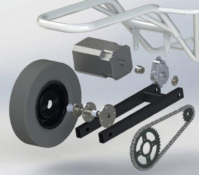

  

  Exploded view of final assembly

8 Analysis

8.1 Modal Analysis

Modal analysis involves the study of dynamic properties of systems in the frequency domain and includes measuring and analyzing the dynamic response of structures during excitation. It also involves the determination of natural frequencies and associated mode shapes of a component or structure under free vibration. The procedure of computerized modal analysis involves:

• Building the model of the component to be analyzed.

• Defining the frequency range followed by meshing.

• Expanding the modes to obtain mode shapes.

• Evaluating the mode shapes and identifying the natural frequency.

8.2 Motor Operating Range

• Minimum speed of motor—0 rpm

• Maximum speed of motor—5000 rpm

• Converting the above into frequency domain, we obtain the motor frequency range to be 0–84 Hz.

8.3 Modal Analysis of Various Components

See Tables 3 and 4, Figs. 21, 22, 23 and 24.

Table 3 Mode frequencies—left and right casing

Table 4 Mode frequencies-driving and driven sprocket

Fig. 21

Modal analysis of left casing

Fig. 22

Modal analysis of right casing

Fig. 23

Modal analysis of the driving sprocket

Fig. 24

Modal analysis of the driven sprocket

Results:

• 1. Six rigid modes are obtained for all the components analyzed.

• 2. Mode frequencies of the components lie outside the range of motor, gears and gearbox frequencies. This ensures resonance-free operation during its service.

8.4 Static Structural Analysis

A static structural analysis determines the stresses, strains, displacements and forces in components primarily caused by loads that do not induce significant inertia and associated damping effects on the component.

8.5 Structural Analysis of Gears

Material properties of EN36C are applied to the gears. The gears are then assembled such that there is contact between the teeth of both gears. It is followed by meshing the gears to an element size of 1 mm. Cylindrical supports are provided for shafts on which bearings are placed. A torque of 28.8 Nm is applied to the shaft connected to the motor shaft.

8.6 Structural Analysis of Gearbox Casing

The major loads acting on the gearbox is through the faces of the bearing pocket. As the current gearbox encloses only spur gears, the axial loads are totally neglected. The radial loads are the ones that are predominant and hence are considered for analysis. The radial load of the gears is taken by the bearings, which in turn transfer these loads to the gearbox casing through the bearing pocket faces. Along with the radial loads, the Chain pull acting through the output shaft is also applied through remote force acting via remote point. These loads are resolved using moment balance equations to find out the respective bearing reaction force and the source of these forces being the gears they act through the center of the shaft (Figs. 25, 26 and 27).

Fig. 25

Stress distribution on the gears

Fig. 26

Stress distribution on gear box

Fig. 27

Loads acting on the bearings

8.7 Structural Analysis of Sprockets and Couplings

Material properties of AISI 1045 are applied to both the sprockets and coupling. They are then meshed to an element size of 1 mm. Fixed supports are provided to the mounting points of the sprocket while cylindrical supports are provided to the portion in contact with the shafts for the couplings. In case of sprockets, torques of 63.6 Nm and 177.6 Nm are applied to the driving and driven sprockets to the portion of the sprocket which is in contact with the chain during its operation. On the other hand, torque is applied on the mounting points of the coupling through which it is connected to the respective sprockets and based on the torque experienced by the respective sprockets, torque values are applied (Figs. 28 and 29).

Fig. 28

Stress distribution on the driven and driving sprockets

Fig. 29

Stress distribution on the sprocket couplings

8.8 Results

Post analysis, it has been observed that all the custom-designed components including gears, couplings, gearbox exhibit safe operating stresses with satisfactory FOS values. The results of the analysis have been mentioned in Table 5.

Table 5 Results of static structural analysis

9 Results and Conclusions

The final outcome was a working prototype of our designed powertrain, which was installed in a tadpole configuration three-wheel vehicle as seen in the images below. When tested, the vehicle was able to achieve speeds of 25–30 kmph and was able to successfully scale a gradient of 15°. There were no issues concerning the power transmission from the motor to the wheels. The prototype is powered by a lead acid battery pack against the desired lithium-ion cells due to the unavailability of the same. For this reason, in the prototype the position of the pillion rider is compromised to accommodate the battery pack. Conclusively it can be said that the vehicle was completed successfully along with the fabrication of a running prototype (Figs. 30 and 31).

Fig. 30

Powertrain assembly with the battery pack

Fig. 31

Prototype testing on campus

References

Łebkowski A (2017) Light electric vehicle powertrain analysis. Sci J Silesian Univ Technol 94:124–137
Lei A et al (2019) A novel approach for electric powertrain optimization considering vehicle power performance, energy consumption and ride comfort. Energy 167:1040–1050
Choi G, Jahns TM (2013) Design of electric machines for electric vehicles based on driving schedules. In: Wisconsin Electric Machines and Power Electronics Consortium (WEMPEC). Madison, Wisconsin, USA
Karamuk M (2011) A survey on electric vehicle powertrain systems. In: International Aegean conference on electrical machines and power electronics and electromotion (ACEMP-Electromotion). Istanbul, Turkey
Balamurugan T, Manoharan S (2014) Design of solar/electric powered hybrid vehicle (SEPHV) system with charge pattern optimization for energy cost. Int J Eng Technol 5(6):4543–4555
Butler KL et al (1999) A Matlab-based modeling and simulation package for electric and hybrid electric vehicle design. Trans Vehicular Technol 48(6):1770–1778
Schönknecht A et al (2016) Electric powertrain system design of BEV and HEV applying a multi objective optimization methodology. In: 6th Transport Research Arena (TRA-2016), vol 14. Warsaw, Poland, pp 3611–3620
Walker PD et al (2013) Modelling, simulations, and optimization of electric vehicles for analysis of transmission ratio selection. Adv Mech Eng 340435
Lee J et al. Development of electric vehicle powertrain: experimental implementation and performance assessment. In: Eighteenth international middle east power systems conference (MEPCON). Cairo, Egypt
Zou Y et al (2012) Optimal energy management strategy for hybrid electric tracked vehicles. Int J Veh Des 58:307–324
Park G et al (2013) Integrated modeling and analysis of dynamics for electric vehicle powertrains. Expert Syst Appl 41(5):2595–2607
Walker P et al (2017) Powertrain dynamics and control of a two speed dual clutch transmission for electric vehicles. Mech Syst Signal Process 85:1–15
Wong JY (2001) Theory of ground vehicles, 3rd edn. Wiley, New York, USA
Jezar RN (2008) Vehicle dynamics: theory and applications. 1 edn. Springer Science + Business Media, LLC – NY, USA
Author information
Authors and Affiliations
Corresponding author
Editor information
Editors and Affiliations
Rights and permissions
Copyright information
© 2022 The Author(s), under exclusive license to Springer Nature Singapore Pte Ltd.
About this paper
Cite this paper
Varadharajan, A.S., Shreekara, R., Salins, S.E., Patil, S.S. (2022). Design and Development of Electric Powertrain for a Proposed Three-Wheel Personal Mobility Vehicle. In: Krishna, V., Seetharamu, K.N., Joshi, Y.K. (eds) Recent Advances in Hybrid and Electric Automotive Technologies. Lecture Notes in Mechanical Engineering. Springer, Singapore. https://doi.org/10.1007/978-981-19-2091-2_13
Download citation
DOI: https://doi.org/10.1007/978-981-19-2091-2_13
Published:
Publisher Name: Springer, Singapore
Print ISBN: 978-981-19-2093-6
Online ISBN: 978-981-19-2091-2
eBook Packages: EngineeringEngineering (R0)