Infobiotics Workbench: An In Silico Software Suite for Computational Systems Biology

Zhang, Gexiang; Pérez-Jiménez, Mario J.; Riscos-Núñez, Agustín; Verlan, Sergey; Konur, Savas; Hinze, Thomas; Gheorghe, Marian

doi:10.1007/978-981-16-1566-5_4

Gexiang Zhang⁸,
Mario J. Pérez-Jiménez⁹,
Agustín Riscos-Núñez⁹,
Sergey Verlan¹⁰,
Savas Konur¹¹,
Thomas Hinze¹² &
…
Marian Gheorghe¹¹

451 Accesses

Abstract

This chapter presents the Infobiotics Workbench (IBW), an integrated software suite developed for computational systems biology. The tool is built upon stochastic P systems, a probabilistic extension of P systems, as modelling framework. The platform utilizes computer-aided modelling and analysis of biological systems through simulation, verification, and optimization. IBW allows modelling and analyzing not only cell-level behavior but also multicompartmental population dynamics. This enables comparing between macroscopic and mesoscopic interpretations of molecular interaction networks and investigating temporospatial phenomena in multicellular systems. These capabilities make IBW a useful, coherent, and comprehensive in silico tool for systems biology research.

Access provided by Autonomous University of Puebla. Download chapter PDF

4.1 Introduction

The modelling and analysis of biological systems using computational approaches alternative to mathematical methods have been the focus of many recent studies since these approaches can reveal more information about system behavior. Various computational formalisms have been introduced and studied in this context, including state transition systems [32], rule-based systems [33], Petri nets [68], and process algebra [59].

Membrane computing is a popular subfield of rule-based systems. Due to its affinity with the functioning and structure of living cells, it has been utilized in modelling and analysis of a number of biological systems [12, 44, 49, 50, 65].

In membrane computing, where models are called P systems , computations represent biological processes that take place within compartments of a living cell. Membrane structures mimic cell structures of living organisms, where compartments contain multisets of objects that evolve by the execution of a set of rules.

Stochastic P systems [64] are a probabilistic variant of P systems, where reaction rates are obtained from elementary rate constants according to the law of mass action kinetics. Stochastic P systems offer a suitable, intuitive, and amenable modeling framework for biological and chemical systems, where the inherent noise that exists in stochastic dynamics of small copy number of systems cannot be properly captured by more traditional mathematical methods. The reaction rules with associated rate constants translate directly and without additional input into probabilistic transitions of the continuous time Markov process that defines the stochastic model.

The Infobiotics Workbench (IBW) is an integrated software suite built upon stochastic P systems models. The platform utilizes computer-aided modelling and analysis of biological systems through a number of important features:

Modelling Language

IBW features a domain-specific language, where individual cells are represented by stochastic P systems. The language also allows specifications of multicellular populations distributed over various geometric surfaces, such as lattices.

Simulation

IBW implements a native stochastic simulator that enables molecular populations to be visualized over cellular populations in space and time. The results can be viewed in different formats, including time series, histograms, and 3D surface plots.

Verification

IBW has a verification component used for validating biological properties. Using powerful probabilistic model checking tools, the platform enables inferring novel system information through formal probabilistic queries and exhaustive analysis of all possible system behaviors.

Optimization

The optimization engine permits optimization parameters by estimating the rate constants in order to converge model dynamics toward laboratory observations. It also optimizes model structures by changing the composition of rule sets managing potential state transitions in compartments to generate alternative reaction networks recreating target dynamics more accurately.

IBW allows modelling and analysis of not only cell-level behavior but also multicompartmental population dynamics. This enables comparing between macroscopic and mesoscopic interpretations of molecular interaction networks and investigating temporospatial phenomena in multicellular systems.

This chapter is divided into the following sections: a presentation of the stochastic P systems, a description of IBW’s key features, two case studies where we illustrate using the IBW features, a short description of a related tool used for qualitative analysis, and finally, a presentation of the next-generation infobiotics for synthetic biology.

4.2 Stochastic P Systems

In IBW, each cell is represented by a stochastic P system (Definition 4.1). The definitions given in this section are borrowed from [12].

Definition 4.1

A stochastic P system (SP system) is a probabilistic variant of P systems, whose semantics is given by a tuple:

$$\displaystyle \begin{aligned} SP=(O,L,\mu,M_1,\dots,M_n,R_1,\dots,R_n) \end{aligned} $$

(4.1)

where:

O is a finite set of objects that specify the entities that are part of the system (such as genes, RNAs, proteins, etc.);
L = {l ₁, …, l _n} is a finite set of labels that name compartments (such as cells, nucleus, cytoplasm, etc.);
μ is a membrane structure containing n ≥ 1 membranes that define the regions or compartments;
M _i = (l _i, w _i, s _i), for each 1 ≤ i ≤ n, is the initial configuration of the membrane i (defining a compartment or a region), where l _i ∈ L is the membrane label, w _i ∈ O ^∗ is a finite multiset of objects, and s _i is a finite set of strings over O;
$R_{l_{k}}=\{r_{1}^{l_{k}},\dots ,r_{m_{l_{k}}}^{l_{k}}\}$, for each 1 ≤ k ≤ n, are a set of multiset rewriting rules that describe molecular interactions, for example, complex formation and gene regulation. Here, each set of rewriting rules $R_{l_{k}}$ are linked to the corresponding compartment identified by the label l _k. The multiset rewriting rules are defined as:
(4.2)

where o ₁, o ₂ and $o_{1}^{\prime },o_{2}^{\prime }$ are multisets of objects (that might be empty), over O, representing molecular species that are consumed/produced in corresponding molecular reactions. The label l (linked to the square brackets) specifies the compartment where the interaction takes place. When such a rule is applied, the contents of the membrane with label l change by replacing the objects o ₂ with $o_{2}^{\prime }$. The contents of the outside membrane also change by replacing the objects o ₁ with $o_{1}^{\prime }$. The stochastic constant $c_{i}^{l_{k}}$ is used to compute the rule propensity (i.e., probability and time required to apply the rule [23]).

Definition 4.1 provides the formal specification for an individual cell. Many biological systems are multicompartmental in nature, that is, they have spatial characteristics in that molecule exchanges between adjacent cells determine overall phenotypes. However, this type of structures cannot be defined by stochastic P systems as these systems have only hierarchical (nested) membrane structures that do not capture multicompartments. Therefore, stochastic P systems should be complemented with a spatial framework. Here, we define such a framework as a two-dimensional geometric lattice, which consists of a population of cells represented by SP systems. Rules moving objects from one cell to another on the lattice are associated with a vector describing where to place these molecules. This geometric extension of stochastic P systems is called lattice population P systems (LPP systems for short) [64].

To capture the spatial distribution of cells forming colonies and tissues, we define a finite point lattice or grid with regularly distributed points [56] that can describe possible spatial geometries in Fig. 4.1. The spatial distribution of cells is defined by a finite point lattice, Definition 4.2.

Definition 4.2

Given B = {v ₁, …, v _n} a list of linearly independent basis vectors, $o\in \mathbb {R}^{n}$ a point referred to as origin, and a list of integer bounds $(\alpha _{1}^{min},\alpha _{1}^{max},$ $\dots ,\alpha _{n}^{min},\alpha _{n}^{max})$, a finite point lattice generated by:

$$\displaystyle \begin{aligned} Lat=(B,o,(\alpha_{1}^{min},\alpha_{1}^{max},\dots,\alpha_{n}^{min},\alpha_{n}^{max})) \end{aligned} $$

(4.3)

is a collection of regularly distributed points, P(Lat), defined as:

$$\displaystyle \begin{aligned} P(Lat)=\{o+\sum_{i=1}^{n}\alpha_{i}v_{i}\;:\;\forall i=1,\dots,n\;(\alpha_{i}\in\mathbb{Z}\wedge\alpha_{i}^{min}\leq\alpha_{i}\leq\alpha_{i}^{max})\} \end{aligned} $$

(4.4)

Given a finite point lattice, generated by Lat, where the coefficients {α _i : i = 1, …, n} uniquely identify each point $x=o+\sum _{i=1}^{n}\alpha _{i}v_{i}\in P(Lat)$, hence denoted as x = (α ₁, …, α _n).

LPP systems allow the distribution of instances of stochastic P systems representing cells on a lattice according to Definition 4.3.

Definition 4.3

A lattice population P (LPP) system is a formal specification of a set of geometrically organized cells, denoted by the following tuple:

$$\displaystyle \begin{aligned} LPP=(Lat,\{SP_{1},\dots,SP_{p}\},Pos,\{T_{1},\dots,T_{p}\}) \end{aligned} $$

(4.5)

where

Lat defines a finite point lattice in $\mathbb {R}^{n}$ (typically n = 2) as in Definition 4.2 describing the geometry of cellular population.
SP ₁, …, SP _p are SP systems as in Definition 4.1 representing different cell types in the population.
Pos : P(Lat) →{SP ₁, …, SP _p} is a function that distributes different instances of SP systems SP ₁, …, SP _p over the lattice points.
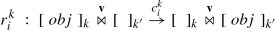
$T_{k}=\{r_{1}^{k},\dots ,r_{n_{k}}^{k}\}$ for each 1 ≤ k ≤ p is a finite set of translocation rules included in the skin membrane of the corresponding SP system SP _k, allowing the interchange of objects between different SP systems located in different geometrical locations. The translocation rules are specified as follows:
(4.6)

where obj is a multiset of objects, v is a vector in $\mathbb {R}^{n}$, and $c_{i}^{k}$ is the stochastic constant. When a translocation rule is applied in the skin membrane of an SP system SP _k located at the point p (Pos(p) = SP _k), the objects obj are removed from this membrane and placed in the skin membrane of $SP_{k'}$ located at the point p + v, $Pos(\mathbf {p}+\mathbf {v})=SP_{k'}$.

In system biology, there are cases where molecular reaction networks can be divided into modules, each of which performs a specific task [27]. It has been shown some modules, called motifs, appear recurrently in transcriptional networks. Motifs carry out particular functions like response acceleration and noise filtering [2].

In order to capture the modularity in LPP systems, hence to be able to model motifs, we have introduced P system modules [12], defined as follows:

Definition 4.4

A P system module, Mod, is defined using three finite ordered sets of variables O = {O ₁, …, O _x}, C = {C ₁, …, C _y}, and Lab = {L ₁, …, L _z} (where O, C and Lab represent objects, stochastic kinetic constants, and compartment labels, respectively). Modules contain a finite set of rewriting rules that have the same form in Eq. (4.2):

$$\displaystyle \begin{aligned} Mod(O,C,Lab)=\{r_{1},\dots,r_{m}\} \end{aligned} $$

(4.7)

O, C, and Lab can be instantiated with specific values o = {o ₁, …, o _x}, c = {c ₁, …, c _y}, and lab = {l ₁, …, l _z} for O, C, and Lab, respectively, as in:

$$\displaystyle \begin{aligned} Mod(\{o_{1},\dots,o_{x}\},\{c_{1},\dots,c_{y}\},\{l_{1},\dots,l_{z}\}) \end{aligned} $$

(4.8)

The rules are generated according to the corresponding substitutions O ₁ = o ₁, …, O _x = o _x, C ₁ = c ₁, …, C _y = c _y and L ₁ = l ₁, …, L _z = l _z.

The use of modularity allows us to define libraries or collections of modules:

$$\displaystyle \begin{aligned} Lib=\{Mod_{1}(O_{1},C_{1},Lab_{1}),\dots,Mod_{p}(O_{p},C_{p},Lab_{p})\} \end{aligned} $$

(4.9)

In order to specify and manipulate LPP system models, we have introduced LPP XML [12], a set of machine-readable data formats closely mirroring our formal definitions. LPP XML allows us to define LPP system models which consist of stochastic P system modules with initial multisets and instantiations of rules and a geometric lattice and distribution of stochastic P systems over the lattice.

The LPP XML formats are very convenient for software implementation, but writing, reading, and manipulating models in XML by hand is a very cumbersome task with syntax obscuring information. Hence, to utilize this process, we have defined a user-friendly DSL (domain-specific language), called LPP DSL. IBW implements a parser that directly reads LPP DSL files and automatically converts them into XML.

The LPP formalism permits the reuse of some components:

Inter-model reuse: Modules (in libraries), stochastic P systems, and lattices are put into different files that can be used and referred from multiple LPP system models.
Intra-model reuse: Multiple SP systems can reside within each LPP system, utilizing the model construction of homogeneous or heterogeneous bacterial colonies or tissues.
Intra-submodel reuse: Modules of rules can be parameterized and instantiated multiple times within an SP system using different instantiations.

P systems modules can be made more or less abstract by parameterizing different elements, such as species and stochastic rate constants. Motifs, corresponding to the topology of the underlying biological network, can be specified by modules that are made fully abstract by representing all components as parameters. In this scenario, parameter names should point out what role their values will play in the module.

4.3 Software Description

The Infobiotics Workbench (IBW) [30] is an integrated in silico platform built upon lattice population P (LPP) systems models [11, 12]. IBW has several functionalities. It allows simulating LPP models using a custom-built stochastic simulator, mcss, and provides a user-friendly dashboard to visualize the simulation experiments in various formats. The dashboard uses adjustable editor views, allowing to edit and run model files easily.

The platform features a model checking component, pmodelchecker, that permits users verify temporospatial dynamic system properties using probabilistic or statistical model checking. IBW also offers parameter and model structure optimization using evolutionary algorithms via POptimizer.

The users can perform experiments using the integrated dashboard or individual components separately outside the workbench. IBW makes the flow of information between different components seamless and easy by passing parameter files and model files through different components (see Fig. 4.2 [12]).

4.3.1 Simulation

The Infobiotics Workbench features a custom-built simulation platform, mcss (multicompartmental stochastic simulation) , comprising two types of quantitative simulations: deterministic numerical approximation with standard solvers and stochastic simulation using Gillespie algorithms [23] . mcss extends the baseline Gillespie method with multicompartmental stochastic algorithms [63] that relies on compartmentalized nature of lattice population P systems models. The algorithm uses queues that store the next rule to execute in each compartment in the heap and only recalculates the reaction propensities in a compartment where a rule is fired. This approach significantly improves performance by reducing the simulation time for models that consist of a large number of compartments.

IBW features a very user-friendly simulation dashboard (see Fig. 4.3) [12]. The simulation environment allows tweaking various simulation parameters, for example, number of runs, time points, and intervals, concentration units, and species to be displayed. The results can be displayed as time series and histograms. System population dynamics can also be observed as surface plotting functions in 3D by selecting a subset of compartments. The results can be exported in common data formats (e.g., csv) for manipulating by third-party software.

The simulation dashboard has a number of features to make the simulation experiments simple, customizable, and reproducible. Users can: (i) select a subset of (or all) entries, multiple, species, and compartments; (ii) filter species or sort them in alphabetical order; (iii) filter compartments or sort them by their geometric positions on the lattice; (iv) adjust simulation time points and intervals; (v) set data and display units (species concentrations as molecules, moles, or concentrations; compartment volumes as liters, milliliter, microliters, and nanoliters; and time points as seconds, minutes, or hours); (vi) select whether species’ amounts in each compartment over the selected runs should be averaged for obtaining approximate results; (vii) get an estimated memory requirement for each simulation experiment to predict how fast the experiment can be carried out; (viii) export the selected and rescaled datapoints in various data formats (.csv, .xls, .npz); and (ix) plot results for selected runs and compartments as time series or histograms, which allows making exact (combined) or relative (stacked/tiled) comparisons of the temporal behavior of different molecular species of same/different compartments based on specific, several, or averaged over many simulation runs. (x) export plots as images for further comparison with experimental observations (see Fig. 4.4) [12]. The figure toolbar enables zooming, panning, and subplot configuration and (xi) visualize the system dynamics at real-time in 2D space using 3D heat-mapped meshes or surface plots to capture the dynamic distribution of selected species over time (see Fig. 4.5) [12]. Surfaces plots provide an intuitive means of qualitative evaluation of population level dynamics that may (cautiously) be compared to laboratory observations.

4.3.2 Verification

Formal methods have been used in systems biology in order to better understand system behavior. As a complementary approach to simulation, formal verification is a method which exhaustively analyzes all possible system behaviors, which cannot be done via simulation, to evaluate the correctness of systems. It allows inferring “more novel information about system properties” [44].

Model checking [14] , an algorithmic verification approach, is used to verify whether a model with a finite structure satisfies certain system properties. Model checking requires a formal system model and a formal specification, expressed in a logical notation [34,35,36,37,38,39]. It then evaluates the formal specification against all possible behaviors of the system model, which are computed by enumerating all possible sequence of traces.

Model checking has been widely utilized in computing and engineering applications for the last two decades in verifying various systems, for example, safety-critical systems [40], concurrent systems [3], distributed systems [69], network protocols [42], stochastic systems [41], multi-agent systems [1, 47], pervasive systems [4, 43, 48], and swarm robotics [45, 46] as well as some engineering applications [57, 58]. Due to its novel features to infer information about system behavior, there is a growing interest to apply this technique in systems biology [8, 9]. Recently, it has been applied to analysis of various biological systems [21, 49, 49, 50, 52, 65].

Probabilistic model checking is a stochastic extension of classical model checking complemented with quantitative techniques to verify properties about the likelihood of the observation of certain behavior. However, they require a probabilistic state machine (such as Discrete-Time Markov Chains (DTMCs), Continuous-Time Markov Chains (CTMCs)) or Markov Decision Processes (MDPs) in a dedicated syntax. System properties are written as probabilistic logical statements, often probabilistic logics: CSL (Continuous Stochastic Logic) [5] for CTMCs and PCTL (Probabilistic Computation Tree Logic) [26] for DTMCs and MDPs. A probabilistic model checker then automatically verifies if the system model satisfies the property using some analytical methods.

The Infobiotics Workbench features a verification module, called pmodelchecker , which integrates two third-party probabilistic models checkers Prism [28] and MC2 [15] . Properties of stochastic P system models are written as probabilistic logic formulas and automatically verified using either Prism or MC2. pmodelchecker extends the verification capability to multicompartments so as to verify LPP system models.

pmodelchecker supports both exact (i.e., numerical) and approximate (i.e., statistical) model checking methods . To perform exact probabilistic model checking, LPP systems are automatically converted into the reactive modules specification, from which Prism is executed. In this approach, the full state space is generated and each property is verified against all states of the model, which is usually computationally very demanding. The approximate probabilistic model checking does not require generating all system states. Instead, simulations are run up to a specified maximum number of runs or a confidence threshold (defined by users), and properties are verified against the simulation traces instead of the system model. To perform approximate probabilistic model checking, users can either (i) call Prism’s discrete event simulator or (ii) run MC2 using previous simulation results or running new simulations.

The pmodelchecker dashboard provides an interface for both Prism and MC2 (see Fig. 4.6) [12]. Users can adjust verification parameters for each model checker, accordingly. The dashboard allows loading multiple formulas from a file and selecting a specific formula that can be edited or removed. Users can also add a new formula using the respective buttons.

The pmodelchecker dashboard features a result view which displays the outcome of a model checking experiment (see Fig. 4.7) [12]. The results can be displayed in 2D if the probability of a property in question is compared against one selected variable, or the results can be displayed in 3D if the probability is checked against two variables. The dashboard allows performing queries that depend on several variables by enabling the choice of variables so that the results of n-dimensional queries to be viewed in a consistent manner.

4.3.3 Optimization

The correct reproduction of cellular behavior depends on the accuracy of kinetic rate constants used in both deterministic and stochastic models. Unfortunately, well-characterized rate constants are not often available in many systems, and those that are known for some models use artificial values that are obtained from similar systems. One possible solution to this problem is using parameter optimization to estimate the rate constants in order to fit model dynamics to laboratory observations.

For this purpose, IBW features the POptimizer component, which optimizes models in two ways:

1.
Numerical model parameters: The stochastic kinetic constants linked to each rule can be tweaked to fit the given target.
2.
Model structure: The composition and structure of the rule sets managing possible state transitions occurring in compartments can be changed to generate alternative reaction networks recreating the target dynamics more accurately.

Both of these optimization steps aim to minimize the distance between the stochastically simulated and user-provided quantities of molecular species at every target time point, quantitatively evaluating the fitness of candidate models and automatically discriminating between them.

POptimizer searches both parameter and structure spaces using well-known population-based optimization algorithms: Covariance Matrix Adaptation Evolution Strategies (CMA-ES) [25], Estimation of Distribution Algorithms (EDA), Differential Evolution (DE) [67], and genetic algorithms (GA) [24]. The current version of the optimization process is limited to single compartment models because multicompartmental structures significantly increase the algorithmic complexity. This is mainly due to the fact that simulating many copies of the cells at those compartments would increase the computational cost and makes it difficult to provide accurate target data. Hence, model optimization is generally feasible for smaller models, which can then be reintegrated, provided they can be decoupled.

POptimizer implements a genetic algorithm [13, 62] to produce candidate models. This is initially done by random choice and then by mutating the fittest models of the previous round, performing several runs of parameter optimization steps on each model to ensure that the candidate models have fair chance of fitting the target behavior before using the final fitness function to choose the next generation.

The result of an optimization process is the fittest model generated, and the outcome is displayed at the dashboard. POptimizer also allows a visual comparison of the quantities of each species for target and the optimized models (see Fig. 4.8) [12].

4.4 Case Studies

In this section, we will illustrate using the IBW features in two case studies. In the first case study, we will use the pulse generator system [10], consisting of a bacterial colony that displays a propagation behavior of a wave of gene expression. The second case study is a genetic circuit, repressilator.

4.4.1 Pulse generator

The pulse generator system [10] synthesizes a signalling molecule AHL, triggering the production of the green fluorescent protein (GFP). The system exhibits a propagation behavior, that is, the propagation of the GFP expression along the bacterial colony (see Fig. 4.11 and 4.12) [12]. The system consists of two different bacterial strains, sender cells and pulsing cells (see Fig. 4.9) [50], which work as follows:

“Sender cells contain the gene luxI from Vibrio fischeri. This gene codifies the enzyme LuxI responsible for the synthesis of the molecular signal 3OC12HSL (AHL). The luxI gene is expressed constitutively under the regulation of the promoter PLtetO1 from the tetracycline resistance transposon.”
Fig. 4.9
The sender and pulsing cells of the pulse generator.
Full size image

Fig. 4.10
Spatial distribution of two bacterial strains
Full size image

Fig. 4.11
Propagation of GFP over a pulsing cell
Full size image

“Pulsing cells contain the luxR gene from Vibrio fischeri that codifies the 3OC12HSL receptor protein LuxR. This gene is under the constitutive expression of the promoter PluxL. It also contains the gene cI from lambda phage codifying the repressor CI under the regulation of the promoter PluxR that is activated upon binding of the transcription factor LuxR_3OC12. Finally, this bacterial strain carries the gene gfp that codifies the green fluorescent protein under the regulation of the synthetic promoter PluxPR combining the Plux promoter (activated by the transcription factor LuxR_3OC12) and the PR promoter from lambda phage (repressed by the transcription factor CI).”

The sender and pulsing bacterial strains are distributed along a lattice, where the sender cells are located at one end of the lattice, and the pulsing cells are placed at the rest of the lattice (see Fig. 4.10).

Modelling

As discussed in Sect. 4.2, IBW accepts lattice population systems as input. The pulse generator system is captured by an LPP model, representing a bacterial colony over a rectangular lattice, which distributes the sender cells at one end of the lattice and the pulsing cells over the rest of the lattice. The LPP model contains two stochastic P systems models, one for each different cell type. The first SP model represents the stochastic behavior of the sender cell, capturing the production of the signal 3OC6-HSL (AHL). The second model represents the pulsing cell, capturing the production of GFP protein as a response to the signal 3OC6-HSL (AHL). In both SP models, the reaction rules govern the regulation of the corresponding promoters used in the sender and pulsing cells. The complete stochastic model of the pulse generator example (written in LPP) is available in the IBW website [60].

References

H. Abbink, R. van Dijk, T. Dobos, M. Hoogendoorn, C. Jonker, S. Konur, P.P. van Maanen, V. Popova, A. Sharpanskykh, P. van Tooren, J. Treur, J. Valk, L. Xu, P. Yolum, Automated support for adaptive incident management, in Proceedings of the 1st International Workshop on Information Systems for Crisis Response and Management (ISCRAM’04) (Brussels, Belgium, 2004), pp. 153–170
R. Alur, K. McMillan, D. Peled, Model-checking of correctness conditions for concurrent objects. Inf. Comput. 160(1–2), 167–188 (2000). https://doi.org/10.1006/inco.1999.2847
M. Arapinis, M. Calder, L. Denis, M. Fisher, P. Gray, S. Konur, A. Miller, E. Ritter, M. Ryan, S. Schewe, C. Unsworth, R. Yasmin, Towards the verification of pervasive systems. Electron. Commun. EASST 22, 1–15 (2009). https://doi.org/10.14279/tuj.eceasst.22.315
C. Baier, B Haverkort, H. Hermanns, J.P. Katoen, Model-checking algorithms for continuous-time markov chains. IEEE Trans. Software Eng. 29, 524–541 (2003). https://doi.org/10.1109/TSE.2003.1205180
M.E. Bakir, F. Ipate, S. Konur, L. Mierlă, I. Niculescu, Extended simulation and verification platform for kernel P systems, in Membrane Computing (CMC 2014), ed. by M. Gheorghe, G. Rozenberg, A. Salomaa, P. Sosík, C. Zandron. Lecture Notes in Computer Science, vol. 8961 (2014), pp. 158–178. https://doi.org/10.1007/978-3-319-14370-5_10
M.E. Bakir, S. Konur, M. Gheorghe, I. Niculescu, F. Ipate, High performance simulations of kernel P systems, in Proceedings of the 2014 IEEE International Conference on High Performance Computing and Communications, 2014 IEEE 6th International Symposium on Cyberspace Safety and Security, 2014 IEEE 11th International Conference on Embedded Software and System (HPCC,CSS,ICESS) (2014), pp. 409–412. https://doi.org/10.1109/HPCC.2014.69
M.E. Bakir, M. Gheorghe, S. Konur, M. Stannett, Comparative analysis of statistical model checking tools, in Membrane Computing (CMC 2016), ed. by A. Leporati, G. Rozenberg, A. Salomaa, C. Zandron. Lecture Notes in Computer Science, vol. 10105 (2017), pp. 119–135. https://doi.org/10.1007/978-3-319-54072-6_8
M.E. Bakir, S. Konur, M. Gheorghe, N. Krasnogor, M. Stannett, Automatic selection of verification tools for efficient analysis of biochemical models. Bioinformatics 34(18), 3187–3195 (2018). https://doi.org/10.1093/bioinformatics/bty282
S. Basu, Y. Gerchman, C.H. Collins, F.H. Arnold, R. Weiss, A synthetic multicellular system for programmed pattern formation. Nature 434 (2005), 1130–1134. https://doi.org/10.1038/nature03461
J. Blakes, J. Twycross, F.J. Romero-Campero, N. Krasnogor, The Infobiotics Workbench: an integrated in silico modelling platform for systems and synthetic biology. Bioinformatics 27(23), 3323–3324 (2011). https://doi.org/10.1093/bioinformatics/btr571
J. Blakes, J. Twycross, S. Konur, F.J. Romero-Campero, N. Krasnogor, M. Gheorghe, Infobiotics workbench: a P systems based tool for systems and synthetic biology, in Applications of Membrane Computing in Systems and Synthetic Biology. Series Emergence, Complexity and Computation, Chapter 7 (2014), pp. 1–41. https://doi.org/10.1007/978-3-319-03191-0_1
H. Cao, F.J. Romero-Campero, S. Heeb, M. Cámara, N. Krasnogor, Evolving cell models for systems and synthetic biology. Syst. Synth. Biol. 4(1), 55–84 (2010). https://doi.org/10.1007/s11693-009-9050-7
R. Donaldson, D. Gilbert, A Monte Carlo model checker for probabilistic LTL with numerical constraints. Res. Rep. (2008), TR-2008-282. Department of Computing Science, University of Glasgow
C. Dragomir, F. Ipate, S. Konur, R. Lefticaru, L. Mierlă, Model checking kernel P systems, in Membrane Computing (CMC 2013), ed. by A. Alhazov, S. Cojocaru, M. Gheorghe, Y. Rogozhin, G. Rozenberg, A. Salomaa. Lecture Notes in Computer Science, vol. 8340 (2013), pp. 151–172. https://doi.org/10.1007/978-3-642-54239-8_12
M.B. Elowitz, S. Leibler, A synthetic oscillatory network of transcriptional regulators. Nature 403(6767), 335–338 (2000). https://doi.org/10.1038/35002125
M. Galdzicki, K.P. Clancy, E. Oberortner, M. Pocock, J.Y. Quinn, C.A. Rodriguez, R. Nicholas, M.L. Wilson, L. Adam, J.C. Anderson, The synthetic biology open language (SBOL) provides a community standard for communicating designs in synthetic biology. Nat. Biotechnol. 32(6), 545–550 (2014). https://doi.org/10.1038/nbt.2891
M. Gheorghe, V. Manca, F.J. Romero-Campero, Deterministic and stochastic P systems for modelling cellular processes. Nat. Comput. 9(2), 457–473 (2009). https://doi.org/10.1007/s11047-009-9158-4
M. Gheorghe, S. Konur, F. Ipate, L. Mierlă, M.E. Bakir, M. Stannett, An integrated model checking toolset for kernel P systems, in Membrane Computing (CMC 2015), ed. by G. Rozenberg, A. Salomaa, J.M. Sempere, C. Zandron. Lecture Notes in Computer Science, vol. 9504 (2015), pp. 153–170. https://doi.org/10.1007/978-3-319-28475-0_11
M. Gheorghe, S. Konur, F. Ipate, Kernel P systems and stochastic P Systems for modelling and formal verification of genetic logic gates, in Advances in Unconventional Computing, ed. by A. Adamatzky. Series Emergence, Complexity and Computation, vol. 22 (2017), pp. 661–675. https://doi.org/10.1007/978-3-319-33924-5_25
M. Gheorghe, R. Ceterchi, F. Ipate, S. Konur, R. Lefticaru, Kernel P systems: from modelling to verification and testing. Theor. Comput. Sci. 724, 45–60 (2018). https://doi.org/10.1016/j.tcs.2017.12.010
D. Gillespie, A general method for numerically simulating the stochastic time evolution of coupled chemical reactions. J. Comput. Phys. 22(4), 403–434 (1976). https://doi.org/10.1016/0021-9991(76)90041-3
A. Hinton, M. Kwiatkowska, G. Norman, D. Parker, Prism: a tool for automatic verification of probabilistic systems, in Tools and Algorithms for the Construction and Analysis of Systems, 12th International Conference, TACAS 2006 Held as Part of the Joint European Conferences on Theory and Practice of Software, ETAPS 2006, Vienna, Austria, March 25—April 2, 2006. Lecture Notes in Computer Science, vol. 3920 (2006), pp. 441–444. https://doi.org/10.1007/11691372_29
M. Hucka, A. Finney, H.M. Sauro, et al. The systems biology markup language (SBML): a medium for representation and exchange of biochemical network models. Bioinformatics 19(4), 524–531 (2002). https://doi.org/10.1093/bioinformatics/btg015
S. Konur, A decidable temporal logic for events and states, in Proceedings of the Thirteenth International Symposium on Temporal Representation and Reasoning (TIME’06), Budapest, 2006 (2006), pp. 36–41. https://doi.org/10.1109/TIME.2006.1
S. Konur, An interval logic for natural language semantics, in Proceedings of the Seventh Conference on Advances in Modal Logic, Nancy, France, 9–12 September 2008, ed. by C. Areces, R. Goldblatt (2008), pp. 177–191
S. Konur, A survey on temporal logics for specifying and verifying real-time systems. Front. Comput. Sci. 7(3), 370–403 (2013). https://doi.org/10.1007/s11704-013-2195-2
S. Konur, Towards light-weight probabilistic model checking. J. Appl. Math. 2014, Article ID 814159, 1–15 (2014). https://doi.org/10.1155/2014/814159
S. Konur, M. Fisher, Formal analysis of a VANET congestion control protocol through probabilistic verification, in Proceedings of the 2011 IEEE 73rd Vehicular Technology Conference (VTC Spring), Yokohama, 2011 (2011), pp. 1–5. https://doi.org/10.1109/VETECS.2011.5956327
S. Konur, M. Gheorghe, A property-driven methodology for formal analysis of synthetic biology systems, in IEEE/ACM Transactions on Computational Biology and Bioinformatics, vol. 12(2), 360–371 (2015). https://doi.org/10.1109/TCBB.2014.2362531
S. Konur, C. Dixon, M, Fisher, Formal verification of probabilistic swarm behaviours, in Swarm Intelligence (ANTS 2010), ed. by M. Dorigo et al. Lecture Notes in Computer Science, vol. 6234 (2010), pp. 440–447. https://doi.org/10.1007/978-3-642-15461-4_42
S. Konur, C. Dixon, M. Fisher, Analysing robot swarm behaviour via probabilistic model checking. Rob. Auton. Syst. 60(2), 199–213 (2012). https://doi.org/10.1016/j.robot.2011.10.005
S. Konur, M. Fisher, S. Schewe, Combined model checking for temporal, probabilistic, and real-time logics. Theor. Comput. Sci. 503, 61–88 (2013). https://doi.org/10.1016/j.tcs.2013.07.012
S. Konur, M. Fisher, S. Dobson, S. Knox, Formal verification of a pervasive messaging system. Formal Aspects Comput. 26(4), 677–694 (2014). https://doi.org/10.1007/s00165-013-0277-4
S. Konur, M. Gheorghe, C. Dragomir, F. Ipate, N. Krasnogor, Conventional verification for unconventional computing: a genetic XOR gate example. Fundam. Inform. 134, 97–110 (2014). https://doi.org/10.3233/FI-2014-1093
S. Konur, M. Gheorghe, C. Dragomir, L. Mierlă, F. Ipate, N. Krasnogor, Qualitative and quantitative analysis of systems and synthetic biology constructs using P systems. ACS Synth. Biol. 4(1), 83–92 (2015). https://doi.org/10.1021/sb500134w
S. Konur, M. Kiran, M. Gheorghe, M. Burkitt, F. Ipate, Agent-based high-performance simulation of biological systems on the GPU, in Proceedings of the 2015 IEEE 17th International Conference on High Performance Computing and Communications, 2015 IEEE 7th International Symposium on Cyberspace Safety and Security, and 2015 IEEE 12th International Conference on Embedded Software and Systems, New York, NY (2015), pp. 84–89. https://doi.org/10.1109/HPCC-CSS-ICESS.2015.253
S. Konur, H. Fellermann, L.M. Mierlă, D. Sanassy, C. Ladroue, S. Kalvala, M. Gheorghe, N. Krasnogor, An integrated in silico simulation and biomatter compilation approach to cellular computation, in Advances in Unconventional Computing, ed. by A. Adamatzky. Series Emergence, Complexity and Computation, vol. 23 (2017), pp. 655–676. https://doi.org/10.1007/978-3-319-33921-4_25
P. Kuhn, K. Wagner, K. Heil, M. Liss, N. Netuschil, Next generation gene synthesis: from microarrays to genomes. Eng. Life Sci. 17(1), 6–13 (2017). https://doi.org/10.1002/elsc.201600121
R. Lefticaru, S. Konur, Ü. Yildirim, A. Uddin, F. Campean, M. Gheorghe, Towards an integrated approach to verification and model-based testing in system engineering, in Proceedings of the 2017 IEEE International Conference on Internet of Things (iThings) and IEEE Green Computing and Communications (GreenCom) and IEEE Cyber, Physical and Social Computing (CPSCom) and IEEE Smart Data (SmartData), Exeter, 2017 (2017), pp. 131–138. https://doi.org/10.1109/iThings-GreenCom-CPSCom-SmartData.2017.25
R. Lefticaru, M.E. Bakir, S. Konur, M. Stannett, F. Ipate, Modelling and validating an engineering application in kernel P systems, in Membrane Computing (CMC 2017), ed. by M. Gheorghe, G. Rozenberg, A. Salomaa, C. Zandron. Lecture Notes in Computer Science, vol. 10725 (2018), pp. 183–195. https://doi.org/10.1007/978-3-319-73359-3_12
F.J. Romero-Campero, H. Cao, M. Camara, N. Krasnogor, Structure and parameter estimation for cell systems biology models, in Proceedings of the 10th Annual Conference on Genetic and Evolutionary Computation (GECCO ’08), Atlanta, GA, USA, July 12–16, 2008 (2008), pp. 331–339. https://doi.org/10.1145/1389095.1389153
F.J. Romero-Campero, J. Twycross, M. Cámara, M. Bennett, M. Gheorghe, N. Krasnogor, Modular assembly of cell systems biology models using P systems. Int. J. Found. Comput. Sci. 20(3), 427–442 (2009). https://doi.org/10.1142/S0129054109006668
F.J. Romero-Campero, J. Twycross, H. Cao, J. Blakes, N. Krasnogor, A multiscale modeling framework based on P systems, in Membrane Computing (WMC 2008), ed. by D.W. Corne, P. Frisco, Gh. Păun, G. Rozenberg, A. Salomaa. Lecture Notes in Computer Science, vol. 5391 (2009), pp. 63–77. https://doi.org/10.1007/978-3-540-95885-7_5
D. Sanassy, H. Fellermann, N. Krasnogor, S. Konur, L. Mierlă, M. Gheorghe, C. Ladroue, S. Kalvala, Modelling and stochastic simulation of synthetic biological Boolean gates, in Modelling and Stochastic Simulation of Synthetic Biological Boolean Gates, 2014 IEEE International Conference on High Performance Computing and Communications, 2014 IEEE 6th International Symposium on Cyberspace Safety and Security, 2014 IEEE 11th International Conference on Embedded Software and Syst (HPCC,CSS,ICESS), Paris, 2014 (2014), pp. 404–408. https://doi.org/10.1109/HPCC.2014.68
K. Sen, M. Viswanathan, G. Agha, Statistical model checking of black-box probabilistic systems, in Computer Aided Verification (CAV 2004), ed. by R. Alur, D.A. Peled. Lecture Notes in Computer Science, vol. 3114 (2004), pp. 202–215. https://doi.org/10.1007/978-3-540-27813-9_16
R. Storn, K. Price, Differential evolution: a simple and efficient heuristic for global optimization over continuous spaces. J. Global Optim. 11, 341–359 (1997). https://doi.org/10.1023/A:1008202821328
F.J.W. Symons, Introduction to numerical Petri nets, a general graphical model of concurrent processing systems. Aust. Telecommun. Res. 14(1), 28–32 (1980)
M. Yabandeh, Model checking of distributed algorithm implementations, Ph.D. thesis, IC (2011). École Polytechnique Fédérale de Lausanne. https://doi.org/10.5075/epfl-thesis-4858
Zhang, G. et al. (2021). Infobiotics Workbench: An In Silico Software Suite for Computational Systems Biology.
In: Membrane Computing Models: Implementations. Springer, Singapore. https://doi.org/10.1007/978-981-16-1566-5_4