Aggregation of LARK Vectors for Facial Image Classification

Abstract

Face recognition is prevailing to be a key aspect wherever there is a need for interaction between humans and machines. This can be achieved by containing a set of sketches for all the possible individuals and then cross-validating at necessary circumstances. We propose a mechanism to fulfil this task which is centred on locally adaptive regression kernels. A comparative study has been presented at encoding stages as well as at the classification stages of the pipeline. The results are cautiously examined and analyzed to deduce the best mechanism out of the proposed methodologies. All the ideologies have been tested for multiple iterations on benchmark datasets like ORL, grimace and faces 95. The vectorized descriptors have been subjected to encoding using slightly refined methods of feature aggregation and clustering to assist classifiers in imputing the test subjects to their respective classes. The encoded vectors are classified using Gaussian Naive Bayes, Stochastic Gradient Descent classifier, linear discriminant analysis and K Nearest Neighbour to accomplish face recognition. An inference on sparse nature of locally adaptive regression kernels was made from the experimentation. A rigorous study regarding the discrepancies of the performance of LARK descriptors is reported.

1 Introduction

Facial recognition is aimed at computing the similar and dissimilar features of an individual by combining the digital image data with the features extracted beforehand. The input image is compared with a library consisting of a collection of images which might not be similar in all respects to the compared image. This image will be contrasted with all the images of the library and then list out a collection of similar images, which often helps us recognise the input image. It can classify the dataset that the image is obtained from. A set of unique and recognisable features are extracted from the images of individuals and are fed into the matchers. This system identifies the nodal points of prime importance. These points act as main features which highlight on primary facets such as the distance and breadth of the nose, the depth of the eye sockets and the measurement of the cheekbones. These systems work by collating data of nodal points on the digital image of an individual’s face and storing the data for further interpretation. These face prints are used as a scale to contrast with data obtained from numerous other faces present in an image or video. A plethora of applications can be tied up to face recognition. Uses include fraud detection in visas and passports, increased security which maps facial data of the card user against ATM’s and banks, tracking of criminals; prevent voters from committing fraud and to maintain a record of attendance.

Conventionally, the security factor is what most facial recognition systems work on. There are several advancements in the field of feature extraction and their description which has spread across multiple domains including face recognition, object detection and automation. These algorithms have played a key role in several applications as well. Consumer digital imaging requires several features to be considered. Putting up with uncontrolled lighting conditions, large pose variations, facial expressions, makeup, changes in facial hair, aging, partial occlusions, loss in pixels and many more parameters can be a tough nut to crack. This paper is an attempt to exhibit a pipeline which is not only computationally inexpensive but highly accurate as well. Locally adaptive regression kernels have proven to be capable descriptors and have shown significant potential to participate in simple and accurate classification models. But selectively aggregating features using a clustering approach is very important to extract feature descriptors for those regions and restrict to regions that is likely to contain specific interest points. Hence the strategy is to find possible clusters in the vector space acquire region descriptors from them and match these vectors based upon their region. The trained classifiers can help us in categorizing these vectors into our interest regions. The proposed pipeline has shown accuracy up to 96% on validation on different benchmark datasets. This paper is an attempt to make a comparative study to explore the properties of LARKs in order to perform facial image classification. A post-processing measure has been implemented on the vectorized LARKs in order to enable us to achieve better results by eliminating overlapping features and obtain more concise results.

Section 2 deals with relevant works that is associated with face recognition and any of the techniques used in the proposed system. Section 3 is an attempt to explain the mechanisms involved in the pipeline to the core. The results are presented and briefly critiqued in the Sect. 4. The outcome of the pipeline is analysed and conclusions are made on the basis of the observations in the Sect. 5.

2 Related Work

Locally adaptive regression kernels [1] have been widely used for non-parametrized training free object detection [2] in a real world application. They have squealed by providing higher accuracy than their counter parts. Several papers used LARK representation of the vectors to achieve face verification within limited amount of computational resources. A popular variant of descriptor called local binary patterns (LBPs) [3] have also shown remarkable outcomes in achieving face recognition. Since LBPs came into light, various version of LBP as three-patch LBP (TPLBP) [4], and four-patch LBP (FPLBP) [5] have been proposed by a different set of individuals. These mapped with the OSS measure helped in growth of “one-shot learning” techniques. Various mechanisms which used learning based descriptors also gained popularity overtime.

The discourse of face verification based on aging effects has been done by Ramanathan and Chelappa with the help of Bayesian and Probabilistic Eigen space [6]. This gave a staggering result with only an average error rate of 8.5%. In [7], Ismail and El-Khoribi with the application of HMT (Hidden Markov Tree) obtained a specification on numerous databases of face images by a of age difference of 5 months which was further divided into 4 junctures. With a range disparity of 20 months, promising results reaching 98% were acquired. An attempt to classify facial images was done by Turk and Pentland using eigen faces [8]. A simple yet affective approach assumed face recognition as two dimensional problems and the frame work designed learned to recognize new faces in an unsupervised manner. Locally adaptive regression kernels have been used for target detection and localization [9] as well. Bag-of-words model, which inspired the design of Bag of lark features model [10], has been used for object recognition by Soon Wei Jun and Safirin Karis. The algorithm learnt new patterns from the code book it creates and learns to classify using those features. Locally-constrained linear coding [11] was used instead of VQ coding in traditional SPM. This performs significantly better than its counter parts on several benchmarks. The time efficiency of LLC helped it to gain popularity in short time. In [12], Zhang and Feng evaluated the performance of naive bayes in text classification applications and gave an improvement over orthodox approach. The new technique exhibited better results that the conventional method.

Chen and Wang focused on achieving multi-face detection system in real time with a bit of hardware acceleration using FPGA [13]. The method used naive bayes for classification and focused on achieving the task using low-memory and in real-time. A slightly different approach was proposed in [14], which combined local features and selected them for naive Bayesian classification. K Nearest neighbour was optimised to objective function based sparse representation to generate locally linear k nearest neighbours (LLK) [15]. The mechanism used two classifiers, an LLK-based classifier and a locally linear nearest mean-based classifier. Novel theoretical analysis was also presented which included the nonnegative constraint, group regularization and also threw light on the computational efficiency of the LLK method. In [16], various classification techniques were benchmarked which helped us rule out the classifiers and limit our study to the one being used in this pipeline. A case study was performed using SVM, KNN, LDA and KNN with PCA along with a thorough analysis of the results to deduce a conclusion of the superiority of the classifiers.

3 Proposed Methodology

3.1 Overview

The region of interest is cropped out from the raw images of an individual to prevent any distortions in the background. As a further measure LARKs are extracted from the images and are converted into vectors by removing overlapping from the raw LARKs which gives a visual impression of the generated LARKs. These vectors act as descriptors of keypoints for the raw image. Eventually they are used for classification and image recognition after aggregation if these features. HOGSVD is then applied to these vectors for the purpose of dimensionality reduction and making them computationally inexpensive. Bag of Lark Features (BOLF) is a clustering algorithm which is used to cluster and compile elements having similar features. Locally constrained linear coding (LLC) is used as a replacement of SPM approach which is on similar grounds as the BOLF. Fischer vectors [17] is an extension of the bag of visual words feature based on visual vocabulary built in low level feature space. This concept is extended to vectors that describe the keypoints. These algorithms make the vectors ready to be fed into classifiers. LDA [18] finds a linear combination of features which selects and classifies objects or lists from analyzed objects. Naive Bayes classifier is based on the conditional probability of classification which uses the previous knowledge obtained. Stochastic Gradient Descent (SGD) is a classification algorithm used to measure analytically the degree of relation two given amongst values or images. Using K nearest neighbors [19] an object is classified based on the majority of votes obtained it’s from its neighbours. These classifiers help to come to a judgement with regards to recognition (Fig. 1).

Fig. 1

Diagrammatic illustration of the pipeline

3.2 Locally Adaptive Regression Kernel (LARK)

Kernel Regression is a non-parametric technique to provide a general idea to the user about the conditional expectation of a completely random variable. The LARK [1] does not require any prior training to identify the image. In normal regression kernels, we usually use spatial differences to weigh the input values. However, in the case of locally adaptive regression kernels, we make use of not only spatial differences but also the difference in data (pixel gradients). Locally adaptive regression kernels denote and represent the local structure of an image taken into consideration. It helps give us a measure of local pixel similarities.

In order to recreate a low quality image on a high resolution image there is a need for a classic regression kernel, for denoising and deblurring the low quality image. The kernel regression framework used in the LARK features is explained as follows:

$$ y_{i} = z\left( {x_{i} +\upvarepsilon_{i} x_{i} \in \omega, \quad i = l \ldots S} \right) $$

(1)

$y_{i}$ is a denoised sample measured at $x_{i} = \left[ {x_{1i} ,x_{2i} } \right]^{T}$ where ${\text{Z}}(x)$ is the required regression function, $\varepsilon_{i}$ is an independently and identically distributed zero mean noise. P is the total number of samples in an arbitrary “window” ω around a position of interest X.

$$ z\left( {x_{i} } \right) \approx z(x) + \left( {\nabla z(x)} \right)^{T} \left( {x_{i } - x} \right) + 1/ 2!\left( {x_{i} - x} \right)^{T} Hz(x)\left( {x_{i} - x} \right) + \cdots $$

(2)

$$ \approx \beta_{0} + \beta_{1}^{T} \left( {x_{i} - x} \right)\beta_{2}^{T} vech\left( {\left( {x_{i} - x} \right)\left( {x_{i} - x} \right)^{T} } \right) + \cdots $$

(3)

where $\nabla$ and H are gradient and Hessian operators, while vech is the half-vectorization operator that lexicographically orders the lower triangular portion of the symmetric matrix into a column stacked vector. $\beta_{1}$ and $\beta_{2}$ can be mathematically defined as:

$$ \beta_{1} = \left[ {\frac{\partial z(x)}{{\partial x_{1} }},\frac{\partial z(x)}{{\partial x_{2} }}} \right]^{T} $$

(4)

$$ \beta_{2} = 1/ 2 \left[ {\frac{{\partial^{2} z(x)}}{{\partial x_{1}^{2} }},\frac{{\partial^{2} z(x)}}{{\partial x_{2}^{2} }}} \right]^{T} $$

(5)

The vech operation can be illustrated as below,

$$ {\text{vech}}\left( {\left[ {\begin{array}{*{20}c} a & b \\ b & d \\ \end{array} } \right]} \right) = \left[ {\begin{array}{*{20}c} a & b & d \\ \end{array} } \right]^{T} $$

$$ {\text{vech}}\left( {\left[ {\begin{array}{*{20}c} a & b & c \\ b & e & f \\ c & f & i \\ \end{array} } \right]} \right) = \left[ {\begin{array}{*{20}c} a & b & c & f & e & i \\ \end{array} } \right]^{T} $$

Locally adaptive regression kernel can be formulated as follows:

$$ K(C_{i} ,x_{i} ,x) = { \exp }\left\{ { - \left( {x_{i} - x} \right)C_{l} \left( {x_{i} - x} \right)} \right\} $$

(6)

where,

$$ C_{i} = \sum\limits_{K \in \omega } {\left[ {\begin{array}{*{20}c} {z_{{x_{1} }}^{2} \left( {x_{k} } \right)} & {z_{{x_{1} }} x(k)z_{{x_{2} }} x(k)} \\ {z_{{x_{1} }} x(k)z_{{x_{2} }} x(k)} & {z_{{x_{2} }}^{2} \left( {x_{k} } \right)} \\ \end{array} } \right]} $$

(7)

Vectorized LARKs act as key points and descriptors for the image. Overlapping patches are removed from the vectorized LARKs, hence giving a visual impression of the generated LARKs. This in turn can be used to plot an image. Different set of key points can be obtained from the pre-processed images by varying smoothness, window size and sensitivity, each time resulting in a slightly different set of vectorized version of LARKs. A unique set of LARKs is obtained every time the parameters are tweaked. Significant variations are observed in the visual LARKs based on the input image. These vectors are later exposed to some dimensionality reduction technique to attain uniformity in processing (Fig. 2).

Fig. 2

a Sample image from database. b Visual LARK with low window size. c Visual LARK with high sensitivity. d Visual LARK with low sensitivity

3.3 Higher-Order Generalized Singular Value Decomposition

The post-processing of these vectors of interest is used to conduct steps that will reduce the complexity and increase the accuracy of the applied algorithm. We cannot write a unique algorithm for each of the condition in which an image is taken, thus, when we acquire an image, we tend to convert it into a form that would allow a general algorithm to solve it. The acquired image is also noisy (inherent in a signal) and thus de-noising it is also a crucial step. Most pre-processing steps that are implemented are either to reduce the noise, to reconstruct an image, to perform morphological operations and to convert the image to binary/greyscale so that operations can be easily implemented on the image. Here HOGSVD will help in reducing the computational intensity and help in escalating the process of feature aggregation (Fig. 3).

Fig. 3

Dimensionality reduction using HOGSVD

This algorithm provides a generalization of the matrix obtained by singular value decomposition for matrices of order N > 2. It is represented as $D_{i} \epsilon R^{m \times n}$ each having a full column rank. Every matrix can be split into components $D_{i} = U_{i} \sum_{i} V^{T}$ where V similar in all its components is acquired from the eigensystem $SV = V\Lambda$ by acquiring the arithmetic mean S of all pairwise quotients of the matrices $A_{i} A_{i}^{T}$, where i ≠ j. It’s eigen values satisfy the inequality $\uplambda_{k} \ge 1$. This equality is valid only if its corresponding eigen vector V_k is a right basis vector of identical significance in all the matrices D_i and D_j where $\upsigma_{i,k} /\upsigma_{j,k} = 1$ for all i and j, and its respective left basis vector U_i,k is orthogonal to all other vectors in U_i for all i.

HOGSVD of these N matrices are:

$$ {\text{D}}_{ 1} = {\text{U}}_{ 1} \sum_{ 1} {\text{V}}^{\text{T}} $$

(8)

$$ {\text{D}}_{ 2} = {\text{U}}_{ 2} \sum_{ 2} {\text{V}}^{\text{T}} $$

(9)

$$ \text{D}_{\text{N}} = {\text{U}}_{\text{N}} \sum_{\text{N}} {\text{V}}^{\text{T}} $$

(10)

$A_{i} = D_{i}^{T} *D_{i}$ equivalently for all $S_{ij}$,

$$ S_{ij} = \frac{1}{2}*\left( {A_{i} *A_{j}^{ - 1} + A_{j} *A_{i}^{ - 1} } \right)\quad {\text{where}}\;i! = j $$

(11)

$$ \begin{aligned} {\text{S}} & = \frac{1}{{N\left( {N - 1} \right)}}\sum\limits_{{i = 1}}^{N} {\sum\limits_{{j > i}}^{N} {\left( {{\text{A}}_{{\text{i}}} {\text{A}}_{{\text{j}}}^{{ - 1}} + {\text{A}}_{{\text{j}}} {\text{A}}_{{\text{i}}}^{{ - 1}} } \right)} } \\ & = \frac{2}{{N\left( {N - 1} \right)}}\sum\limits_{{i = 1}}^{N} {\sum\limits_{{j > i}}^{N} {{\text{S}}_{{{\text{ij}}}} } } \\ \end{aligned} $$

(12)

$SV = V\Lambda$ where $S = \left( {v_{1} \ldots v_{n} } \right)$ and $\Lambda = diag\left( {lambda_{k} } \right)$.

Characteristics and applications of HOGSVD include:

• 1. HOGSVD is used to the extract the key information from multi-way arrays. Data analysis, recognition and synthesis problems are multilinear tensor problems based on the fact that most data that is observed are results of several causal factors of data formation, and are well suited for multi-modal data tensor analysis.

• 2. Currently it is being used in signal processing and big data which includes genomic signal processing.

• 3. Collation of HOSVD and SVD has been applied to detect real time events which are obtained from complex data streams.

• 4. HOGSVD was considered one of the best to be applied to multi-view data analysis and was successfully applied to discover silico drug from gene expression (Fig. 4).

  Fig. 4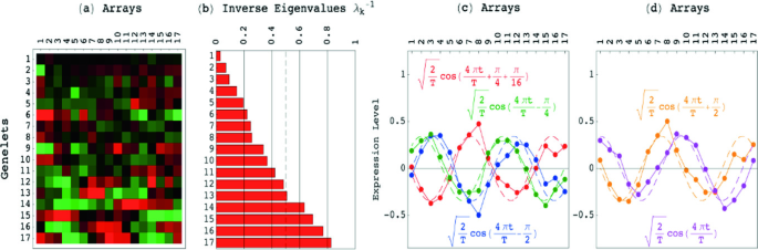

  

  Overview of the process

Once the vectorized LARKs are prepared for feature aggregation, the set of vectors are processed using Bag of LARK features, LLC and Fischer vectors.

3.4 Feature Aggregation

3.4.1 Bag of LARK Features

The bag of LARK features is a logical way of representing data while modelling the dataset with various processing algorithms. It is a clustering algorithm which compiles elements of similar features. However, these clustering algorithms cannot work with the raw image which we consider as an input. It must be represented as a kernel after multiplying the Kernel RBF—PCS with the locally adaptive regression Kernel (LARK).

The bag of LARK features is a way of extracting a particular feature from a dataset of input features present in a codebook. It is called as a “bag” of LARK features as any information about the origin of the vector in the plain space is disregarded. It is only concerned whether the particular variable occurs in the cluster present in the code book.

In the Bag of LARK Features model which we have considered, the set of local variables from the vectorized version of the locally adaptive regression kernel into the final set of images is done in a succession of two steps: Clustering and Pooling.

• 1. Clustering: The clustering part in the original Bag of LARK Features model is the formation of clusters consisting of similar vectors when the vectorized model of the locally adaptive regression kernel is plotted. Since this low-level combination has a large impact on performance, the results are reported to be over 40% similarity for images with pre-processing done and up to 90% similarity for images which have not undergone any pre-processing.

• 2. Pooling: Once the clustering is finished and we have obtained a new locally adaptive regression kernel with every vector replaced with the special vector from the cluster, all images from the data set are plotted once more and the same processes is repeated to obtain images with a higher level of accuracy. The algorithm involving a combination of these two features is the Bag of LARK features algorithm (Fig. 5).

  Fig. 5

  

  Cluster Dendrogram from bag of LARK features

Using this algorithm, the user can extract images similar to the input image fed from the given dataset. The Bag of LARK features is a novel scheme of image classification using mid-level parameters such as codebooks and normalization. The codebooks are the most significant parameters as they allow to group images with a richer density to obtain more accurate results.

3.4.2 Locally Constrained Linear Coding (LLC)

The locally constrained linear coding is a clustering technique which is simple but extremely effective. It can be used as a suitable replacement to the SPM approach based on the bag-of-features (BoF) approach which requires non-linear classifiers to achieve a good image classification performance.

The locally constrained linear coding algorithm constraints to project each of the image descriptor which is the vectorized form of the locally adaptive regression kernel (LARK) for our case into its local database system. The projected co-ordinate vectors are then max-pooled to generate the final representation of the image.

Let X be a set of D Dimensional local descriptors extracted from an image. i.e. $X = \left[ {x_{1}, x_{2}, \ldots, x_{n} } \right] \in {\mathbb{R}}^{D \times N}$. Given a codebook with M entries from the image vectors of locally adaptive regression kernel considered, $B = \left[ {b_{1}, b_{2}, \ldots, b_{m} } \right] \in {\mathbb{R}}^{D \times M}$. Different coding schemes convert each image descriptor into M-Dimensional code to generate the final image representation.

The locally constrained linear coding incorporates the locality constraint instead of the sparsity constraint which leads to several favourable properties. Specifically, the LLC uses the following criteria:

$$ { \hbox{min} }\sum\limits_{i = 0}^{n} {\left\| {x_{i} - B_{ci} x^{2} + \lambda } \right\|} \left. {d_{i} \odot C_{i} } \right\| $$

(13)

where ${ \circledcirc }$ denotes element wise multiplication and $d_{i} \in IR^{M}$ is locality adaptor that gives freedom for each basis vector.

The locally constrained linear coding algorithm is preferred as it provides a superior image classification performance compared to other clustering or classification techniques.

Once we process the images using the Bag of LARK Features algorithm and the Locally Constrained Linear Coding algorithms, we then teach the computer the datasets which we have considered in the paper. The classification and identification of the data input image is done using the proposed techniques.

3.4.3 Fischer Vectors

The Fisher Vector (FV) representation of images can be seen as an extension of the popular bag-of-visual word (BOV). Both of them are based on an intermediate representation, the visual vocabulary built in the low-level feature space. If a probability density function (in our case a Gaussian Mixture Model) is used to model the visual vocabulary, we can compute the gradient of the log likelihood with respect to the parameters of the model to represent an image. The Fisher Vector is the concatenation of these partial derivatives and describes in which direction the parameters of the model should be modified to best fit the data. This representation has the advantage to give similar or even better classification performance than BOV obtained with supervised visual vocabularies, being at the same time class independent.

We model the visual vocabulary with a Gaussian mixture model (GMM) where each Gaussian corresponds to a visual word. Let $\lambda = \left\{ {\omega_{i} ,\mu_{i} ,\sum i,\;i = 1 \ldots N} \right\}$ be the set of parameters of p where $\omega_{i}$, $\mu_{i}$, $\sum i$ denote the weight, mean vector and covariance matrix in the LARK.

$$ p\left( {x |\lambda } \right) = \sum\limits_{i = 1}^{N} {\omega_{i} p_{i} \left( {x |\lambda } \right)} = \sum\limits_{i = 1}^{N} {\omega_{i} N\left( {x|\mu_{i} \sum i} \right)} $$

(14)

Let $\left\{ {x_{t}, x_{t}, \in {\mathbb{R}}^{D}, t = 1 \ldots T} \right\}$ be the set of local descriptors of the image, then by using Baye’s formula we have.

$$ \gamma_{i} \left( {x_{t} } \right) = \frac{{\omega_{i} p_{i} \left( {x |\lambda } \right)}}{{\mathop \sum \nolimits_{j = 1}^{N} \omega_{j} p_{j} \left( {x |\lambda } \right)}} $$

(15)

In the BOV representation, the low-level descriptor is hence transformed into a high level N-dimensional descriptor.

$$ \gamma_{t} = \left[ {\gamma_{1} x_{t} ,\gamma_{2} x_{t} , \ldots ,\gamma_{n} x_{t} ,} \right] $$

(16)

where $\sum\nolimits_{n = 1}^{N} {\gamma_{n} x_{t} = 1}$ is an accumulation of these probabilities over low level descriptors.

3.5 Classifiers

3.5.1 Stochastic Gradient Descent

The Stochastic Gradient Descent (SGD) is basically an optimization algorithm which is used to calculate analytically the degree of relation between two given data values or images for the particular case that we have considered. It has a simple goal to best estimate a target function (f) that maps input data (x) onto output variable (y). It also describes the basic algorithm of all classification and regression problems. It provides a process of optimization to find the set of coefficients that result in the best estimate of the target file. Gradient descent is a slow technique which cannot often be run on very large datasets because of the time constraints. In these cases, we use the Stochastic Gradient Descent. Usually, every descent of the gradient algorithm has a prediction for each instance in the dataset. This is not recommended as there maybe millions of instances present. However, in case of the Stochastic Gradient Descent, update to the coefficients is performed for each training instance rather than at the end of the batch of the data instances. It utilises a single new sample data in each iteration and processes the end data in a stream-like fashion. SGD optimization is linearly scalable in time and the computational time can be sped up to two or three times in magnitude.

Consider a supervised learning model, where we are given a set of samples $\left( {a,b} \right) \in A \times B$ taken from the probability distribution $P\left( {a,b} \right)$. The conditional probability represents the relation between the input variable a and the output variable b. The difference between the estimated variable $\hat{b}$ and the true variable b is represented by a loss function $l\left( {b,b} \right)$. Using SGD algorithm, we try to estimate the function f that minimises this expected risk.

$$ E(f) = \int {l\left( {f(a),b} \right)dP\left( {a,b} \right) = {\mathbb{E}}\left[ {l\left( {f{\{ }a ),b} \right)} \right]} $$

(17)

Due to its incremental behaviour, SGD has features that support online adaptation of classification functions and a classification model that is available at any given point of time. This enables us to give complete solutions in cases where the time constraints do not allow us to give a retraining of the classification model (Fig. 6).

Fig. 6

Tuning alpha value in stochastic gradient descent using a plot

3.5.2 Gaussian Naive Bayes

A Naive Bayes is a classifier with an inbuilt powerful algorithm for the classification of millions of data files and records with only a limited number of attributes. The Bayes theorem is an integral part of the Naive Bayes classification system. It is based on conditional probability which is calculating the probability of an even occurring based on prior knowledge. The formulae for calculating conditional probability can be explained as follows:

$$ P\left( {H |E} \right) = \frac{{P\left( {E |H} \right)*P\left( H \right)}}{P\left( E \right)} $$

(18)

where,

• $P\left( H \right)$ is the probability of the hypothesis H being true

• $P\left( E \right)$ is the probability of evidence.

• $P(E|H)$ is probability of evidence given that the hypothesis is true.

• $P(H|E)$ is probability of hypothesis given evidence is present.

The Naive Bayes classifier predicts the probabilities for each of the class that is considered such as the probability of the given data or record belongs to a particular class. Hence the class with the highest probability is considered as the most likely class. When an image is processed and the features are extracted, the Naive Bayes naturally assumes that all features are unrelated to each other. One feature being present or absent does not affect any other feature in any way.

Gaussian Naive Bayes is a particular type of Naive Bayes algorithm that considers all the attribute values to be continuous and an assumption is made that all the values associated with each other are grouped into a Normal Distribution. The basic theorem upon which the Gaussian Naive Bayes algorithm works is given as:

$$ P\left( {x_{i } |y} \right) = \frac{1}{{\sqrt {2\pi \sigma_{y}^{2} } }}{ \exp }\left( { - \frac{{\left( {x_{i} - \mu_{y} } \right)^{2} }}{{2\sigma_{y}^{2} }}} \right) $$

(19)

The Gaussian Naive Bayes algorithm [17] is a fast and reliable algorithm that can be used for Binary and Multiclass classification. It can also be easily trained on a small dataset but is not recommended for a larger dataset due to the time constraints. It can also deal with missing attributes in a given data file. Consider a set of image files that we have taken as an input, here each image is represented by an individual vector representation called as the Bag of LARK Features representation. We then fit the Gaussian Naive Bayes algorithm by initially teaching a dataset to the computer memory and then the target elements are classified by comparing them with the elements implemented into the database.

3.5.3 Fischer Linear Discriminant Analysis

Fischer Linear Discriminant Analysis or commonly known as Linear Discriminant Analysis [20] is a classification technique that is used in statistics, pattern recognition and machine learning to find a linear combination of features which selects or classifies objects or lists from the analysed objects. The transformation is based on maximizing mean square error between original data vectors and data vectors that can be estimated from the reduced dimensionality vectors (Fig. 7).

Fig. 7

LDA on a custom dataset

The left plot shows the samples from two classes along with the histograms resulting from the projection onto the line joining the class means. The right plot shows the corresponding projection based on the Fischer linear discriminant, showing the greatly improved class separation.

Assume we have a set of D-dimensional samples $X = \left\{ {x^{(1)} ,x^{(2)} , \ldots x^{(m)} } \right\},N_{1}$ of which belong to class $C_{1}$ and $N_{2}$ of which belong to class $C_{2}$. We also assume the mean vector of the two classes in X-space.

$$ u_{k} = \frac{1}{{N_{k} }}\sum\limits_{{i \in C_{k} }} {x^{(i)} } \quad where\;k = 1,2, \ldots . $$

(20)

And in y-space:

$$ \hat{u}_{k} = \frac{1}{{N_{k} }}\sum\limits_{{i \in C_{k} }} {\theta^{T} x^{(i)} } = \theta^{T} u_{k} \quad where\;k = 1,2, \ldots $$

(21)

One way to define a measure of separation between two classes is to choose the distance between the projected means, which is in y-space, so the between class variance is:

$$ \hat{u}_{2} - \hat{u}_{1} = \theta^{T} \left( {u_{2} - u_{1} } \right) $$

(22)

Also, we define the within–class variance for each class $C_{k}$ is:

$$ \hat{s}_{k}^{2} = \mathop \sum \limits_{{i \epsilon C_{k} }} \left( {y^{(i)} - \hat{u}_{k} } \right)^{2} \quad where\;k = 1,2, \ldots $$

(23)

Then, we get the between-class variance and within-class variance; we can define our objective function $J\left( \theta \right)$ as:

$$ J\left( \theta \right) = \frac{{\left( {\hat{u}_{2} - \hat{u}_{1} } \right)}}{{\hat{s}_{1}^{2} + \hat{s}_{2}^{2} }}^{2} $$

(24)

If maximising the objective function J, we are looking for a projection where examples from the class are projected very close to each other and at the same time, the projected means are as farther apart as possible.

For the Multi-Classes Problems we see that the fisher’s LDA generalizes gracefully. Assuming we still have a set of D-dimensional samples $X = \left\{ {x^{(1)} ,x^{(2)} , \ldots x^{(m)} } \right\}$ and there are totally C classes. Instead of one projection y as mentioned we will seek $\left( {C - 1} \right)$ projections where:

$$ y_{i} = \theta_{i}^{T} X \Rightarrow y =\Theta ^{\text{T}} {\text{X}} $$

(25)

We will use the scatters in space-x as follows:

Within-class scatter matrix:

$$ \begin{aligned} S_{W} & = \sum\limits_{i = 1}^{C} {S_{i} } \quad where\;S_{i} = \sum\limits_{{i \in C_{i} }} {\left( {x^{{(i) - u_{i} }} } \right)} \left( {x^{i} - u_{i} } \right)^{T} , \\ u_{i} & = \frac{1}{{N_{i} }}\sum\limits_{{i \in C_{i} }} {x^{(i)} } \\ \end{aligned} $$

(26)

Between-Class scatter matrix:

$$ S_{B} = \sum\limits_{i = 1}^{C} {N_{i} } \left( {u_{i} - u} \right)\left( {u_{i} - u} \right)^{T} \quad where\,u = \frac{1}{m}\sum\limits_{i = 1}^{m} {x^{(i)} } = \frac{1}{m}\sum\limits_{i = 1}^{C} {N_{i} u_{i} } $$

(27)

Total scatter matrix:

$$ S_{T} = S_{B} + S_{W} $$

(28)

3.5.4 K Nearest Neighbours

This is a non-parametric methodology to perform classification and regression. Input comprises of k-nearest examples which are to be trained in feature space. Output is either the one obtained by classification or regression. It works on the principle of representative based learning where approximation on the function is discharged provincially and the resulting calculation is often delayed in unit organisation. The neighbours are obtained from a collection of objects where the category of the class, the property and value of the object is familiar in nature.

The tuples (A, B),(A₁, B₁), …, (A_n, B_n) where the values are in R^d*{1, 2}, B being the class identifier for A the equation is given by:

$$ \frac{A}{B} = r \sim P_{r} \quad where\;r = 1,2, \ldots $$

(29)

Here P_r denotes a probability distribution.

By interchanging the tuples (A₍₁₎B₍₁₎), …, (A_(n)B_(n)) in a way that ||A_{1} − a|| $\Leftarrow \cdots \Leftarrow$||A_{n} − a||.

The similarity of KNN is obtained by measuring the distance between two points using distance metrics between data points. The Euclidean distance is given by the equation:

$$ d\left( {x,x^{{\prime }} } \right) = (\left( {x_{1} - x_{1}^{{\prime }} } \right)^{2} + \left( {x_{2} - x_{2}^{{\prime }} } \right)^{2} + \cdots + \left( {x_{n} - x_{n}^{{\prime }} } \right)^{2} )^{{\frac{1}{2}}} $$

(30)

From the above graph the boundary between the red and blue interface becomes smoother for increasing values of k. As the value of k tends to infinity it becomes either blue or red in colour depending completely upon the larger proportion (Fig. 8).

Fig. 8

KNN output for different values of k on a custom dataset

3.6 Datasets and Experimentation

To test the righteousness of the methodology for variations, corresponding datasets were used. They helped in the testing and the analysis of the methodology that was used in the paper.

3.6.1 ORL Faces

Formerly known as ‘The ORL Dataset of Faces’, the dataset holds images from the early 1990s captured at the Cambridge University Computer Laboratory. It contains ten unique images of 40 different individuals, subjected to various variations such as the time of capture of the image, lighting of the images, facial expressions of the individuals and other accessories worn by the individuals. Each of the images has a standard 92 × 112 pixels with a set 256 grey levels per unit. The dataset was a unique dataset as lots of different image variations were considered while taking the images.

The image is quantized to 256 grey levels and stored as unsigned 8-bit integers; the loader will convert these to floating point values on the interval [0, 1], which are easier to work with for many algorithms. The “target” for this database is an integer from 0 to 39 indicating the identity of the person pictured; however, with only 10 examples per class, this relatively small dataset is more interesting from an unsupervised or semi-supervised perspective (Fig. 9).

Fig. 9

A sample ORL dataset

3.6.2 Grimace

This unique dataset is an assembly of 18 different individuals designed and maintained by Dr. Libor Spacek. Grimace [20] has a main objective to focus on variations between male and female candidates. The dataset contains 20 portraits of each of the candidate considered at a resolution of 180 × 200 pixels. The background is kept same throughout all the images with small uniform head scale variations. The lighting changes are minimal and little to no variations in hairstyle of the considered candidates (Fig. 10).

Fig. 10

A sample Grimace faces dataset

3.6.3 Faces95

Once again, a Brain Child [21] of Dr. Libor Spacek, this particular dataset contains portraits of 72 different and distinct subjects. Sequences of 20 images were captured while the subject was asked to step towards the camera after every snap that was taken. This kind of a special dataset offers a huge head scale variation and minor variations due to the difference in the depth of the shadows that is varied each time the subject takes a step towards the camera. This results in a discrepancy in red background. Noticeable changes in lighting occur due to the artificial lighting systems used.

4 Results and Inference

The results obtained are presented below in a concise manner in the table that is shown in Table 1.

Table 1 Results obtained from ORL dataset

Accuracy assessment is an important path of any classification project. It compares an input image with another image that is present in the dataset which is classified and gives an accurate report of the matching between the two images that have been considered. Recall is also known as sensitivity in image processing and classification. It is the fraction of relevant instances that have been taken or considered in the total instances that are present in the dataset. It is basically a measure of relevance. Following observations were made from the obtained values during experimentation.

• 1. LARK needs a lot of variance in the data. Any preprocessing done to the input image is likely to affect the result of the classification.

• 2. Some data sets like the FACE95 datasets have low precision/recall because they do not have a lot of variations or variables when compared to the other datasets

• 3. The challenges that are offered by the datasets need to be handled better and all the variables need to be considered. Only then we will be able to achieve the precision and accuracy that we require.

Out of three feature aggregation techniques LLC always yielded poor results compared to other two techniques. We can deduce that LLC is not a suitable pair for clustering of LARK vectors. Bag of LARK features showed remarkable results on several iterations for all the datasets with an aggregate of over 15% better accuracy than other techniques. It was clearly observed that HOGSVD as a post processing step did not help much in increasing the accuracy. On an average all the combinations of aggregation mechanism and classifiers yielded 10% higher accuracy without HOGSVD. This proves that the dimensionality reduction does lead to loss of features and LARKs give high covariance values in all the dimensions. The precision as well as recall was exceptionally high for grimace dataset which proves that the pipeline can handle changes in facial expressions very well. The results for ORL dataset was just above average for any combination. This reflects that the pipeline does not perform well when the region of interest shift is small or the distortions in the background are very high. There is a scope making the pipeline completely scale and orientation invariant as ORL does offer head scale and orientation invariance to certain extent. Out of all the classifiers LDA performed outstanding with every combination the pipeline has to offer.

5 Conclusion and Future Work

Locally Adaptive Regression Kernels have proven to be capable descriptors. It can be concluded that LARK descriptors are sparse in nature and are suffice themselves. Any form of processing to achieve dimensionality reduction will lead to degeneration of features and degrade the performance of the system. They show little to no variance on repeated trails and give high accuracy when paired with different classifiers. From the experimentation, it is deduced that any form of pre-processing or post-processing in the form of dimensionality reduction or denoising does lead to loss of features and declined accuracy. The methodology requires feature rich images and loss of data in any form is not tolerated by the mechanism. Feature aggregation helped us in clustering the vectors into groups, similar to our interests. Since the regional descriptors were procured from the constructed clusters vectors using these aggregated vectors for classification yielded better results.

A comparative study performed has shown that Bag of LARK features and stochastic gradient descent comprise the best combination in the pipeline used. It was observed that LLC delivered lesser accuracy when paired with Higher-Order generalized singular value decomposition. Grimace dataset posed least challenges to the system and consistently provided very good results on several iterations of the mechanism. The other classifiers performed up to the mark on faces95, while ORL dataset delivered harder set of challenges.

The need for a better algorithm with respect to pre-processing the images is of high prominence. A suitable algorithm which denoises the image without the loss of significant features is essential. The model looks promising and can deliver better results if worked on. There is scope for better classifiers as well. Future work includes pairing these post-processed LARKs with artificial neural networks for better classification, designing an algorithm for pre-processing the images before using locally adaptive kernels on them. The encoding system which aggregates the features can elevate the rightness if worked on.

References

Seo, H.J., Milanfar, P.: Face verification using the LARK representation. IEEE Trans. Inf. Forensics Secur. 6(4), 1275–1286 (2011)
Meena, K., Suruliandi, A.: Local binary patterns and its variants for face recognition. In: 2011 International Conference on Recent Trends in Information Technology (ICRTIT), Chennai, Tamil Nadu, pp. 782–786 (2011)
Hadid, A.: The local binary pattern approach and its applications to face analysis. In: 2008 First Workshops on Image Processing Theory, Tools and Applications, Sousse, pp. 1–9 (2008)
Ahonen, T., Hadid, A., Pietikainen, M.: Face description with local binary patterns: application to face recognition. IEEE Trans. Pattern Anal. Mach. Intell. 28(12), 2037–2041 (2006)
Ramanathan, N., Chellappa, R.: Face verification across age progression. IEEE Trans. Image Process. 15(11), 3349–3361 (2006)
Osman, A.A.E., El-Khoribi, R.A., Shoman, M.E., Shalaby, M.A.W.: Trajectory learning using posterior hidden Markov model state distribution. Egypt. Inform. J. (2017)
Turk, M.A., Pentland, A.P.: Face recognition using eigenfaces. In: Proceedings of IEEE Conference Computer Vision and Computer Vision (CVPR), pp. 586–591 (1991)
He, K., Zhou, D., Nie, R., Jin, X., Wang, Q.: Image specific target detection and localization based on locally adaptive regression kernels algorithm. In: 2016 8th IEEE International Conference on Communication Software and Networks (ICCSN), Beijing, pp. 647–651 (2016)
Ali, N.M., Jun, S.W., Karis, M.S., Ghazaly, M.M., Aras, M.S.M.: Object classification and recognition using Bag-of-Words (BoW) model. In: 2016 IEEE 12th International Colloquium on Signal Processing & Its Applications (CSPA), Malacca City, pp. 216–220 (2016)
Wang, J., Yang, J., Yu, K., Lv, F., Huang, T., Gong, Y.: Locality-constrained Linear Coding for image classification. In: 2010 IEEE Computer Society Conference on Computer Vision and Pattern Recognition, San Francisco, CA, pp. 3360–3367 (2010)
Zhang, W., Gao, F.: Performance analysis and improvement of naïve Bayes in text classification application. In: IEEE Conference Anthology, China, pp. 1–4 (2013)
Chen, Y.P., Liu, C.H., Chou, K.Y., Wang, S.Y.: Real-time and low-memory multi-face detection system design based on naive Bayes classifier using FPGA. In: 2016 International Automatic Control Conference (CACS), Taichung, pp. 7–12 (2016)
Ouarda, W., Trichili, H., Alimi, A.M., Solaiman, B.: Combined local features selection for face recognition based on Naïve Bayesian classification. In: 13th International Conference on Hybrid Intelligent Systems (HIS 2013), Gammarth, pp. 240–245 (2013)
Liu, Q., Liu, C.: A novel locally linear KNN method with applications to visual recognition. IEEE Trans. Neural Netw. Learn. Syst. 28(9), 2010–2021 (2017)
Parveen, P., Thuraisingham, B.: Face recognition using multiple classifiers. In: 2006 18th IEEE International Conference on Tools with Artificial Intelligence (ICTAI’06), Arlington, VA, pp. 179–186 (2006)
Uchida, Y., Sakazawa, S.: Image retrieval with fisher vectors of binary features. In: 2013 2nd IAPR Asian Conference on Pattern Recognition, Naha, pp. 23–28 (2013)
Chelali, F.Z., Djeradi, A., Djeradi, R.: Linear discriminant analysis for face recognition. In: 2009 International Conference on Multimedia Computing and Systems, Ouarzazate, pp. 1–10 (2009)
Taneja, S., Gupta, C., Goyal, K., Gureja, D.: An enhanced K-nearest neighbor algorithm using information gain and clustering. In: 2014 Fourth International Conference on Advanced Computing & Communication Technologies, Rohtak, pp. 325–329 (2014)
Putranto, E.B., Situmorang, P.A., Girsang, A.S.: Face recognition using eigenface with Naive Bayes. In: 2016 11th International Conference on Knowledge, Information and Creativity Support Systems (KICSS), Yogyakarta, pp. 1–4 (2016)
Dr Libor SpaceK.: Collection of Facial Images: Grimace (Online) (2007). Retrieved from: http://cswww.essex.ac.uk/mv/allfaces/grimace.html
Dr Libor SpaceK.: Collection of Facial Images: Faces95 (Online) (2007). Retrieved from:http://cswww.essex.ac.uk/mv/allfaces/faces95.html
Author information
Authors and Affiliations
Corresponding author
Editor information
Editors and Affiliations
Rights and permissions
Copyright information
© 2020 Springer Nature Singapore Pte Ltd.
About this paper
Cite this paper
Vinay, A., Kamath, V.R., Varun, M., Nidheesh, Natarajan, S., Murthy, K.N.B. (2020). Aggregation of LARK Vectors for Facial Image Classification. In: Manna, S., Datta, B., Ahmad, S. (eds) Mathematical Modelling and Scientific Computing with Applications. ICMMSC 2018. Springer Proceedings in Mathematics & Statistics, vol 308. Springer, Singapore. https://doi.org/10.1007/978-981-15-1338-1_31
Download citation
DOI: https://doi.org/10.1007/978-981-15-1338-1_31
Published:
Publisher Name: Springer, Singapore
Print ISBN: 978-981-15-1337-4
Online ISBN: 978-981-15-1338-1
eBook Packages: Mathematics and StatisticsMathematics and Statistics (R0)