Analytics Models for Data Science

Abstract

The ultimate goal of data science is to turn raw data into data products. Data analytics is the science of examining the raw data with the purpose of making correct decisions by drawing meaningful conclusions.

3.1 Introduction

The ultimate goal of data science is to turn raw data into data products. Data analytics is the science of examining the raw data with the purpose of making correct decisions by drawing meaningful conclusions. The key differences of traditional analytics versus Big Data Analytics are shown in Table 3.1.

Table 3.1 Traditional analytics versus Big Data Analytics

3.2 Data Models

Data model is a process of arriving at the diagram for deep understanding, organizing and storing the data for service, access and use. The process of representing the data in a pictorial format helps the business and the technology experts to understand the data and get to know how to use the data. This section deals with data science and four computing models of data analytics.

3.2.1 Data Products

Data products define which type of profiles would be desirable to deliver the resultant data products that are collected during data gathering process. Data gathering normally involves collecting unstructured data from various sources. As an example, this process could involve acquiring raw data or reviews from a web site by writing a crawler. Three types of data products are as follows:

• Data used to predict,

• Data used to recommend,

• Data used to benchmark.

3.2.2 Data Munging

Data munging, sometimes referred to as data wrangling, is the process of converting and mapping data from one format (raw data) to another format (desired format) with the purpose of making it more suitable, easier and valuable for analytics. Once data retrial is done from any source, for example, from the web, it needs to be stored in an easy to use format. Suppose a data source provides reviews in terms of rating in stars (1–5 stars); this can be mapped with the response variable of the form x ∈ {1, 2, 3, 4, 5}. Another data source provides reviews using thumb rating system, thumbs-up and thumbs-down; this can be inferred with a response variable of the form x ∈ {positive, negative} (Fig. 3.1). In order to make a combined decision, first data source response (five-point star rating) representation has to be converted to the second form (two-point logical rating), by considering one and two stars as negative and three, four and five stars as positive. This process often requires more time allocation to be delivered with good quality.

Fig. 3.1

Thumb and star rating system

3.2.3 Descriptive Analytics

Descriptive analytics is the process of summarizing historical data and identifying patterns and trends. It allows for detailed investigation to response questions such as ‘what has happened?’ and ‘what is currently happening?’ This type of analytics uses historical and real-time data for insights on how to approach the future. The purpose of descriptive analytics is to observe the causes/reasons behind the past success or failure.

The descriptive analysis of data provides the following:

• Information about the certainty/uncertainty of the data,

• Indications of unexpected patterns,

• Estimates and summaries and organize them in graphs, charts and tables and

• Considerable observations for doing formal analysis.

Once the data is grouped, different statistical measures are used for analyzing data and drawing conclusions. The data was analyzed descriptively in terms of

• 1. Measures of probability,

• 2. Measures of central tendency,

• 3. Measures of variability,

• 4. Measures of divergence from normality,

• 5. Graphical representation.

A measure of central tendency indicates the central value of distribution which comprises mean, median and mode. However, the central value alone is not adequate to completely describe the distribution. We require a measure of the spread/scatter of actual data besides the measures of centrality. The standard deviation is more accurate to find the measure of dispersion. The degree of dispersion is measured by the measures of variability, and that may vary from one distribution to another. Descriptive analysis is essential by the way it helps to determine the normality of the distribution. A measure of divergence from normality comprises standard deviation, skewness and kurtosis. A measure of probability includes standard error of mean and fiduciary limits used to set up limits for a given degree of confidence. Statistical techniques can be applied for inferential analysis, to draw inferences/ make predictions from the data. Graphic methods are used for translating numerical facts into more realistic and understandable form.

3.2.4 Predictive Analytics

Predictive analytics is defined to have data modeling for making confident predictions about the future or any unknown events using business forecasting and simulation which depends upon the observed past occurrences. These address the questions of ‘what will happen?’ and ‘why will it happen?’

Predictive model uses statistical methods to analyze current and historical facts for making predictions [1]. Predictive analytics is used in actuarial science, capacity planning, e-commerce, financial services, insurance, Internet security, marketing, medical and health care, pharmaceuticals, retail sales, transportation, telecommunications, supply chain and other fields. Applications of predictive analytics in business intelligence comprise customer segmentation, risk assessment, churn prevention, sales forecasting, market analysis, financial modeling, etc.

Predictive modeling process is divided into three phases: plan, build and implement. Planning includes scoping and preparing. Predictive modeling process for a wide range of businesses is depicted well in Fig. 3.2.

Fig. 3.2

Predictive modeling process

To build a predictive model, one must set clear objectives, cleanse and organize the data, perform data treatment including missing values and outlier fixing, make a descriptive analysis of the data with statistical distributions and create datasets used for the model building. This may take around 40% of the overall time. The subphases of build the model are model and validate. Here, you will write model code, build the model, calculate scores and validate the data. This is the part that can be left with the data scientists or technical analysts. This might take around 20% of the overall time. The subphases of action are deploy, assess and monitor. It involves deploy and apply the model, generate ranking scores for customers or products (most popular product), use the model outcomes for business purpose, estimate model performance and monitor the model. This might take around 40% of the overall time.

Sentiment analysis is the most common model of predictive analytics. This model takes plain text as input and provides sentiment score as output which in turn determines whether the sentiment is neutral, positive or negative. The best example of predictive analytics is to compute the credit score that helps financial institutions like banking sectors to decide the probability of a customer paying credit bills on time. Other models for performing predictive analytics are

• Time series analysis,

• Econometric analysis,

• Decision trees,

• Naive Bayes classifier,

• Ensembles,

• Boosting,

• Support vector machines,

• Linear and logistic regression,

• Artificial neural network,

• Natural language processing,

• Machine learning.

3.2.5 Data Science

Data science is a field associated with data capturing, cleansing, preparation, alignment and analysis to extract information from the data to solve any kind of problem. It is a combination of statistics, mathematics and programming. One way of assessing how an organization currently interacts with data and determines where they fit to achieve increasingly accurate hindsight, insight and foresight and its different ecosystems in four fundamental ways [2] (i) descriptive analytics, (ii) diagnostic analytics, (iii) predictive analytics and (iv) prescriptive analytics by Gartner’s analytics maturity model is illustrated in Fig. 3.3.

Fig. 3.3

Gartner’s analytics maturity model

The four types of analytics [3] and their association along with the dimensions from rule-based to probability-based and the dimensions of time (past, present and future) are depicted in Fig. 3.4.

Fig. 3.4

Four types of analytics

The focus of the top left and the bottom right quadrants, i.e., diagnostic and prescriptive analytics, is past and future, while the focus of the bottom left and top right quadrants, i.e., descriptive and predictive analytics, is past and future. The summary is provided in Table 3.2.

Table 3.2 Key differences of four types of analytics

Consider an example of the story of The Jungle Book. Baloo a bear hired a data analyst (Mowgli) to help find his food honey. Mowgli had access to a large database, which consisted of data about the jungle, road map, its creatures, mountains, trees, bushes, places of honey and events happening in the jungle. Mowgli presented Baloo with a detailed report summarizing where he found honey in the last six months, which helped Baloo decide where to go for hunting next; this process is called descriptive analytics.

Subsequently, Mowgli has estimated the probability of finding honey at certain places with a given time, using advanced machine learning techniques. This is predictive analytics. Next, Mowgli has identified and presented the areas that are not fit for hunting by finding their root cause why the places are not suitable. This is diagnostic analytics. Further, Mowgli has explored a set of possible actions and suggested/recommended actions for getting more honey. This is prescriptive analytics. Also, he identified shortest routes in the jungle for Baloo to minimize his efforts in finding food. This is called as optimization. We already had enough discussion on descriptive and predicative analytics; further let go through the explanatory details of diagnostic and prescriptive analytics.

Diagnostic Analytics

It is a form of analytics which examines data to answer the question ‘why did it happen?’ It is kind of root cause analysis that focuses on the processes and causes, key factors and unseen patterns.

Steps for diagnostic analytics:

• (i) Identify the worthy problem for investigation.

• (ii) Perform the Analysis: This step finds a statistically valid relationship between two datasets, where the upturn or downturn occurs. Diagnostic analytics can be done by the following techniques

  • Multiregression,

  • Self-organizing maps,

  • Cluster and factor analysis,

  • Bayesian clustering,

  • k-nearest neighbors,

  • Principal component analysis,

  • Graph and affinity analysis.

• (iii) Filter the Diagnoses: Analyst must identify the single or at most two influential factors from the set of possible causes.

Prescriptive Analytics

This model determines what actions to take in order to change undesirable trends. Prescriptive analytics is defined as deriving optimal planning decisions given the predicted future and addressing questions such as ‘what shall we do?’ and ‘why shall we do it?’ Prescriptive analytics is based on [4]

• Optimization that helps achieving the best outcomes,

• Stochastic optimization that helps understanding how to identify data uncertainties to make better decisions and accomplish the best outcome.

Prescriptive analytics is a combination of data, business rules and mathematical models. It uses optimization and simulation models such as sensitivity and scenario analysis, linear and nonlinear programming and Monte Carlo simulation.

3.2.6 Network Science

In networked systems, standardized graph-theoretic methods are used for analyzing data. These methods have the assumption that we precisely know the microscopic details such as how the nodes are interconnected with each other. Mapping network topologies can be costly, time consuming, inaccurate, and the resources they demand are often unaffordable, because the datasets comprised billions of nodes and hundreds of billions of links in large decentralized systems like Internet. This problem can be addressed by combining methods from statistical physics and random graph theory.

The following steps are used for analyzing large-scale networked systems [5]:

• Step 1: To compute the aggregate statistics of interest. It includes the number of nodes, the density of links, the distribution of node degrees, diameter of a network, shortest path length between pair of nodes, correlations between neighboring nodes, clustering coefficient, connectedness, node centrality and node influence. In distributed systems, this can be computed and estimated efficiently by sensible sampling techniques.

• Step 2: To determine the statistical entropy ensembles. This can be achieved by probability spaces by assigning probabilities to all possible network realizations that are consistent with the given aggregate statistics using analytical tools like computational statistics methods of metropolis sampling.

• Step 3: Finally, derive the anticipated properties of a system based on aggregate statistics of its network topology.

3.3 Computing Models

Big data grows super-fast in four dimensions (4Vs: volume, variety, velocity and veracity) and needs advanced data structures, new models for extracting the details and novel algorithmic approach for computation. This section focuses on data structure for big data, feature engineering and computational algorithm.

3.3.1 Data Structures for Big Data

In big data, special data structures are required to handle huge dataset. Hash tables, train/atrain and tree-based structures like B trees and K-D trees are best suited for handling big data.

Hash table

Hash tables use hash function to compute the index and map keys to values. Probabilistic data structures play a vital role in approximate algorithm implementation in big data [6]. These data structures use hash functions to randomize the items and support set operations such as union and intersection and therefore can be easily parallelized. This section deals with four commonly used probabilistic data structures: membership query—Bloom filter, HyperLogLog, count–min sketch and MinHash [7].

Membership Query—Bloom filter

A Bloom filter proposed by Burton Howard Bloom in 1970 is a space-efficient probabilistic data structure that allows one to reduce the number of exact checks, which is used to test whether an element is ‘a member’ or ‘not a member’ of a set. Here, the query returns the probability with the result either ‘may be in set’ or ‘definitely not in set.’

Bit vector is the base data structure for a Bloom filter. Each empty Bloom filter is a bit array of ‘m’ bits and is initially unset.

0	0	0	0	0	0	0	0	0	0	0	0	0
0	1	2	3	4	5	6	7	8	9	10	11	12

When an element is added to the filter, it is hashed by ‘k’ functions, h₁, h₂ … h_k mod by ‘m’, resulting in ‘k’ indices into the bit array, and the respective index is set to ‘1’ [8]. Figure 3.5 shows how the array gets updated for the element with five distinct hashing functions h₁, h₂, h₃, h₄ and h₅.

Fig. 3.5

Bloom filter hashing

To query the membership of an element, we hash the element again with the same hashing functions and check if each corresponding bit is set. If any one of them is zero, then conclude the element is not present.

Suppose you are generating an online account for a shopping Web site, and you are asked to enter a username during sign-up; as you entered, you will get an immediate response, ‘Username already exists.’ Bloom filter data structure can perform this task very quickly by searching from the millions of registered users.

Consider you want to add a username ‘Smilie’ into the dataset and five hash functions, h₁, h₂, h₃, h₄ and h₅ are applied on the string. First apply the hash function as follows

• h₁(“Smilie”)%13 = 10

• h₂(“Smilie”)%13 = 4

• h₃(“Smilie”)%13 = 0

• h₄(“Smilie”)%13 = 11

• h₅(“Smilie”)%13 = 6

Set the bits to 1 for the indices 10, 4, 0, 11 and 6 as given in Fig. 3.6.

Fig. 3.6

Bloom filter after inserting a string ‘Smilie’

Similarly, enter the next username ‘Laughie’ by applying the same hash functions.

• h₁(“Laughie”)%13 = 3

• h₂(“Laughie”)%13 = 5

• h₃(“Laughie”)%13 = 8

• h₄(“Laughie”)%13 = 10

• h₅(“Laughie”)%13 = 12

Set the bits to 1 for the indices 3, 5, 8, 10 and 12 as given in Fig. 3.7.

Fig. 3.7

Bloom filter after inserting a string ‘Laughie’

Now check the availability of the username ‘Smilie’ is presented in filter or not. For performing this task, apply hashing using h₁, h₂, h₃, h₄ and h₅ functions on the string and check if all these indices are set to 1. If all the corresponding bits are set, then the string is ‘probably present.’ If any one of them indicates 0, then the string is ‘definitely not present.’

Perhaps you will have a query, why this uncertainty of ‘probably present’, why not ‘definitely present’? Let us consider another new username ‘Bean.’ Suppose we want to check whether ‘Bean’ is available or not. The result after applying the hash functions h₁, h₂, h₃, h₄ and h₅ is as follows

• h₁(“Bean”)%13 = 6

• h₂(“Bean”)%13 = 4

• h₃(“Bean”)%13 = 0

• h₄(“Bean”)%13 = 11

• h₅(“Bean”)%13 = 12

If we check the bit array after applying hash function to the string ‘Bean,’ bits at these indices are set to 1 but the string ‘Bean’ was never added earlier to the Bloom filter. As the indices are already set by some other elements, Bloom filter incorrectly claims that ‘Bean’ is present and thus will generate a false-positive result (Fig. 3.8).

Fig. 3.8

Bloom filter for searching a string ‘Bean’

We can diminish the probability of false-positive result by controlling the size of the Bloom filter.

• More size/space decrease false positives.

• More number of hash functions lesser false positives.

Consider a set element A = {a₁, a₂, …, a_n} of n elements. Bloom filter defines membership information with a bit vector ‘V’ of length ‘m’. For this, ‘k’ hash functions, h₁, h₂, h₃ … h_k with $h_i{:}\,X\{ 1 \ldots m\}$, are used and the procedure is described below.

• Procedure BloomFilter (a_i elements in set Arr, hash-functions h_j, integer m)

• filter = Initialize m bits to 0

  • foreach a_i in Arr:

    • foreach hash-function h_j:

      • filter[h_j(a_i)] = 1

    • end foreach

  • end foreach

• return filter

Probability of false positivity ‘P’ can be calculated as:

$$P = \left( {1 - \left[ {1 - \frac{1}{m}} \right]^{kn} } \right)^{k}$$

where

• ‘m’ is the size of bit array,

• ‘k’ is the number of hash functions and

• ‘n’ is the number of expected elements to be inserted.

Size of bit array ‘m’ can be calculated as [9]:

$$m = \frac{n\ln P}{{(\ln 2)^{2} }}$$

Optimum number of hash functions ‘k’ can be calculated as:

$$k = \frac{m}{n}\ln 2$$

where ‘k’ must be a positive integer.

Cardinality—HyperLogLog

HyperLogLog (HLL) is an extension of LogLog algorithm derived from Flajolet–Martin algorithm (1984). It is a probabilistic data structure used to estimate the cardinality of a dataset to solve the count-distinct problem, approximating the number of unique elements in a multiset. It required an amount of memory proportional to the cardinality for calculating the exact cardinality of a multiset, which is not practical for huge datasets. HLL algorithm uses significantly less memory at the cost of obtaining only an approximation of the cardinality [10]. As its name implies, HLL requires O(log₂log₂n) memory where n is the cardinality of the dataset.

HyperLogLog algorithm is used to estimate how many unique items are in a list. Suppose a web page has billions of users and we want to compute the number of unique visits to our web page. A naive approach would be to store each distinctive user id in a set, and then the size of the set would be considered by cardinality. When we are dealing with enormous volumes of datasets, counting cardinality by the said way will be ineffective because the dataset will occupy a lot of memory. But if we do not need the exact number of distinct visits, then we can use HLL as it was designed for estimating the count of billions of unique values.

Four main operations of HLL are:

• 1. Add a new element to the set.

• 2. Count for obtaining the cardinality of the set.

• 3. Merge for obtaining the union of two sets.

• 4. Cardinality of the intersection.

• HyperLogLog [11]

  • def add(cookie_id: String): Unit

  • def cardinality( ):

    • //$\left| A \right|$

  • def merge(other: HyperLogLog):

    • //$\left| {A \cup B} \right|$

  • def intersect(other: HyperLogLog):

    • //$\left| {A \cap B} \right| = \left| A \right| + \left| B \right| - \left| {A \cup B} \right|$

Frequency—Count–Min sketch

The count–min sketch (CM sketch) is a probabilistic data structure which is proposed by G. Cormode and S. Muthukrishnan that assists as a frequency table of events/elements in a stream of data. CM sketch maps events to frequencies using hash functions, but unlike a hash table it uses only sublinear space to count frequencies due to collisions [12]. The actual sketch data structure is a matrix with w columns and d rows [13]. Each row is mapped with a hash function as in Fig. 3.9.

Fig. 3.9

Count–min data structure

Initially, set all the cell values to 0.

0	0	0	0	0	0	0	0
0	0	0	0	0	0	0	0
0	0	0	0	0	0	0	0
0	0	0	0	0	0	0	0
0	0	0	0	0	0	0	0

When an element arrives, it is hashed with the hash function for each row and the corresponding values in the cells (row d and column w) will be incremented by one.

Let us assume elements arrive one after another and the hashes for the first element f₁ are: h₁(f₁) = 6, h₂(f₁) = 2, h₃(f₁) = 5, h₄(f₁) = 1 and h₅(f₁) = 7. The following table shows the matrix current state after incrementing the values.

Let us continue to add the second element f₂, h₁(f₂) = 5, h₂(f₂) = 1, h₃(f₂) = 5, h₄(f₂) = 8 and h₅(f₂) = 4, and the table is altered as

In our contrived example, almost element f₂ hashes map to distinct counters, with an exception being the collision of h₃(f₁) and h₃(f₂). Because of getting the same hash value, the fifth counter of h₃ now holds the value 2.

The CM sketch is used to solve the approximate Heavy Hitters (HH) problem [14]. The goal of HH problem is to find all elements that occur at least n/k times in the array. It has lots of applications.

• 1. Computing popular products,

• 2. Computing frequent search queries,

• 3. Identifying heavy TCP flows and

• 4. Identifying volatile stocks.

As hash functions are cheap to compute and produce, accessing, reading or writing the data structure is performed in constant time. The recent research in count–min log sketch which was proposed by G. Pitel and G. Fouquier (2015) essentially substitutes CM sketch linear registers with logarithmic ones to reduce the relative error and allow higher counts without necessary to increase the width of counter registers.

Similarity—MinHash

Similarity is a numerical measurement to check how two objects are alike. The essential steps for finding similarity are: (i) Shingling is a process of converting documents, emails, etc., to sets, (ii) min-hashing reflects the set similarity by converting large sets to short signature sets, and (iii) locality sensitive hashing focuses on pairs of signatures likely to be similar (Fig. 3.10).

Fig. 3.10

Steps for finding similarity

MinHash was invented by Andrei Broder (1997) and quickly estimates how similar two sets are. Initially, AltaVista search engine used MinHash scheme to detect and eliminate the duplicate web pages from the search results. It is also applied in association rule learning and clustering documents by similarity of their set of words. It is used to find pairs that are ‘near duplicates’ from a large number of text documents. The applications are to locate or approximate mirror web sites, plagiarism check, web spam detection, ordering of words, finding similar news articles from many news sites, etc.

MinHash provides a fast approximation to the Jaccard similarity [15]. The Jaccard similarity of two sets is the size of their intersection divided by size of their union (Fig. 3.11).

Fig. 3.11

Jaccard similarity

$$J(A,B) = \frac{{\left| {A \cap B} \right|}}{{\left| {A \cup B} \right|}}$$

If the sets are identical, then J = 1; if they do not share any member, then J = 0; if they are somewhere in between, then 0 ≤ J ≤ 1.

MinHash uses hashing function to quickly estimate Jaccard similarities. Here, the hash function (h) maps the members of A and B to different integers. hmin(S) finds the member ‘x’ that results the lowest of a set S. It can be computed by passing every member of a set S through the hash function h. The concept is to condense the large sets of unique shingles into much smaller representations called ‘signatures.’ We can use these signatures alone to measure the similarity between documents. These signatures do not give the exact similarity, but the estimates they provide are close.

Consider the below input shingle matrix where column represents documents and rows represent shingles.

Define a hash function h as by permuting the matrix rows randomly. Let perm1 = (12345), perm2 = (54321) and perm3 = (34512). The MinHash function hmin(S) = the first row in the permuted order in which column C has ‘1’; i.e., find the index that the first ‘1’ appears for the permuted order.

For the first permutation Perm1 (12345), first ‘1’ appears in column 1, 2 and 1. For the second permutation Perm2 (54321), first ‘1’ appears in column 2, 1 and 2. Similarly for the third permutation Perm3 (34512), first ‘1’ appears in column 1, 3 and 2. The signature matrix [16] after applying hash function is as follows.

Perm1 = (12345)	1	2	1
perm2 = (54321)	2	1	2
perm3 = (34512)	1	3	2

The similarity of signature matrix can be calculated by the number of similar documents (s)/no. of documents (d). The similarity matrix is as follows.

	1, 2	1, 3	2, 3
col/col $\left( {\frac{{\left| {A \cap B} \right|}}{{\left| {A \cup B} \right|}}} \right)$	0/5 = 0	2/4 = 0.5	1/4 = 0.25
sig/sig (s/d)	0/3 = 0	2/3 = 0.67	0/3 = 0

The other representation (the same sequence of permutation will be considered for calculation) of signature matrix for the given input matrix is as follows:

Perm1 = (12345)	1	2	1
perm2 = (54321)	4	5	4
perm3 = (34512)	3	5	4

Another way of representing signature matrix for the given input matrix is as follows. Consider 7 × 4 input matrix with three permutations after applying hash functions, perm1 = (3472615), perm2 = (4213675), perm3 = (2376154), and the corresponding 3 × 4 signature matrix is given in Fig. 3.12. Here, the signature matrix is formed by elements of the permutation based on first element to map a ‘1’ value from the element sequence start at 1. First row of the signature matrix is formed from the first element 1 with row value (1 0 1 0). Second element 2 with row values (0 1 0 1) can replace the above with (1 2 1 2). The row gets completed if there is no more ‘0’s. Second row of the signature matrix is formed from the first element (0 1 0 1) which will be further replaced as (2 1 0 1), and then third column ‘0’ is updated with 4 since fourth element of the permutation is the first to map ‘1’.

Fig. 3.12

Min-hashing

With min-hashing, we can effectively solve the problem of space complexity by eliminating the sparseness and at the same time preserve the similarity.

Tree-based Data Structure

The purpose of a tree is to store naturally hierarchical information, such as a file system. B trees, M trees, R trees (R*, R+ and X tree), T trees, K-D trees, predicate trees, LSM trees and fractal tree are the different forms of trees to handle big data.

B trees are efficient data structure for storing big data and fast retrieval. It was proposed by Rudolf Bayer for maintaining large database. In a binary tree, each node has at most two children, and time complexity for performing any search operation is O(log₂ N). B tree is a variation of binary tree, which is a self-balancing tree, each node can have M children, where M is called fan-out or branching factor, and because of its large branching factor it is considered as one of the fastest data structures. It thus attains a time complexity of O(log_M N) for each search operation.

B tree is a one-dimensional index structure that does not work well and is not suitable for spatial data because search space is multidimensional. To resolve this issue, a dynamic data structure R tree was proposed by Antonin Guttman in 1982 for the spatial searching. Consider massive data that cannot fit in main memory. When the number of keys is high, the data is read in the form of blocks from the disk. So, disk access time is higher than main memory access time. The main motive of using B trees is to decrease the number of disk accesses by using a hierarchical index structure. Internal nodes may join and split whenever a node is inserted or deleted because range is fixed. This may require rebalancing of tree after insertion and deletion.

The order in B tree is defined as the maximum number of children for each node. A B tree of order ‘n’ (Fig. 3.13) has the following properties [17]:

• 1. A B tree is defined by minimum degree ‘n’ that depends upon the disk block size.

• 2. Every node has maximum ‘n’ and minimum ‘n/2’ children.

• 3. A non-leaf node has ‘n’ children, and it contains ‘n − 1’ keys.

• 4. All leaves are at the same level.

• 5. All keys of a node are sorted in increasing order. The children between two keys ‘k1’ and ‘k2’ contain the keys in the range from ‘k1’ and ‘k2’.

• 6. Time complexity to search, insert and delete in a B tree is O(log_M N).

  Fig. 3.13

  

  A B tree of order 5

K-D Trees

A K-D tree or K-dimensional tree was invented by Jon Bentley in 1970 and is a binary search tree data structure for organizing some number of points in a ‘K’-dimensional space. They are very useful for performing range search and nearest neighbor search. K-D trees have several applications, including classifying astronomical objects, computer animation, speedup neural networks, data mining and image retrieval.

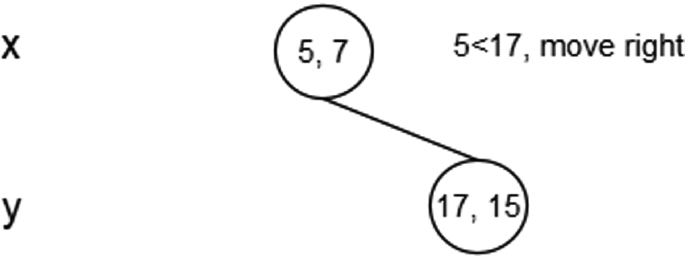
The algorithms to insert and search are same as BST with an exception at the root we use the x-coordinate. If the point to be inserted has a smaller x-coordinate value than the root, go left; otherwise go right. At the next level, we use the y-coordinate, and then at the next level we use the x-coordinate, and so forth [18].

Let us consider the root has an x-aligned plane, then all its children would have y-aligned planes, all its grandchildren would have x-aligned planes, all its great-grandchildren would have y-aligned planes and the sequence alternatively continues like this. For example, insert the points (5, 7), (17, 15), (13, 16), (6, 12), (9, 1), (2, 8) and (10, 19) in an empty K-D tree, where K = 2. The process of insertion is as follows:

• Insert (5, 7): Initially, as the tree is empty, make (5, 7) as the root node and X-aligned.

  

• Insert (17, 15): During insertion firstly compare the new node point with the root node point. Since root node is X-aligned, the X-coordinate value will be used for comparison for determining the new node to be inserted as left subtree or right subtree. If X-coordinate value of the new point is less than X-coordinate value of the root node point, then insert the new node as a left subtree else insert it as a right subtree. Here, (17, 15) is greater than (5, 7), this will be inserted as the right subtree of (5, 7) and is Y-aligned.

  

• Insert (13, 16): X-coordinate value of this point is greater than X-coordinate value of root node point. So, this will lie in the right subtree of (5, 7). Then, compare Y-coordinate value of this point with (17, 15). As Y-coordinate value is greater than (17, 15), insert it as a right subtree.

  

• Similarly insert (6, 12).

  

• Insert other points (9, 1), (2, 8) and (10, 19).

The status of 2-D tree after inserting elements (5, 7), (17, 15), (13, 16), (6, 12), (9, 1), (2, 8) and (10, 19) is given in Fig. 3.14 and the corresponding plotted graph is shown in (Fig. 3.15).

Fig. 3.14

2-D tree after insertion

Fig. 3.15

K-D tree with a plotted graph

• Algorithm for insertion

• Insert (Keypoint key, KDTreeNode t, int level)

• {

  • typekey key[];

  • if (t = = null)

    • t = new KDTreeNode (key)

  • else if (key = = t.data)

    • Error // Duplicate, already exist

  • else if (key[level] < t.data[level])

    • t.left = insert (key, t.left, (level + 1) % D)

  • else

    • t.right = insert (key, t.right, (level + 1) % D)

    • //D-Dimension;

  • return t

• }

The process of deletion is as follows: If a target node (node to be deleted) is a leaf node, simply delete it. If a target node has a right child as not NULL, then find the minimum of current node’s dimension (X or Y) in right subtree, replace the node with minimum point, and delete the target node. Else if a target node has left child as not NULL, then find minimum of current node’s dimension in left subtree, replace the node with minimum point, delete the target node, and then make the new left subtree as right child of current node [19].

• Delete (5, 7): Since right child is not NULL and dimension of node is x, we find the node with minimum x value in right subtree. The node (6, 12) has the minimum x value, and we replace (5, 7) with (6, 12) and then delete (5, 7) (Fig. 3.16).

  Fig. 3.16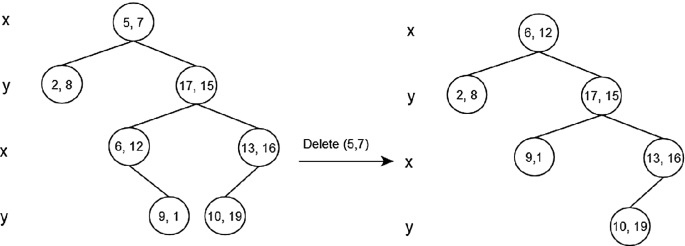

  

  K-D tree after deletion of X-coordinate point

• Delete (17, 15): Since right child is not NULL and dimension of node is y, we find the node with minimum y value in right subtree. The node (13, 16) has a minimum y value, and we replace (17, 15) with (13, 16) and delete (17, 15) (Fig. 3.17).

  Fig. 3.17

  

  K-D tree after deletion of Y-coordinate point

• Delete (17, 15)—no right subtree: Since right child is NULL and dimension of node is y, we find the node with minimum y value in left subtree. The node (9, 1) has a minimum y value, and we replace (17, 15) with (9, 1) and delete (17, 15). Finally, we have to modify the tree by making new left subtree as right subtree of (9, 1) (Fig. 3.18).

  Fig. 3.18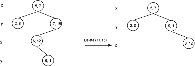

  

  K-D tree after deletion of Y-coordinate point with NULL right tree

• Algorithm for finding a minimum

• Algorithm for deletion:

K-D trees are useful for performing nearest neighbor (NN) search and range search. The NN search is used to locate the point in the tree that is closest to a given input point. We can get k-nearest neighbors, k approximate nearest neighbors, all neighbors within specified radius and all neighbors within a box. This search can be done efficiently by speedily eliminating large portions of the search space. A range search finds the points lie within the range of parameters.

Train and Atrian

Big data in most of the cases deals with heterogeneity types of data including structured, semi-structured and unstructured data. ‘r-train’ for handling homogeneous data structure and ‘r-atrain’ for handling heterogeneous data structure have been introduced exclusively for dealing large volume of complex data. Both the data structures ‘r-train’ (‘train,’ in short) and ‘r-atrain’ (‘atrain,’ in short), where r is a natural number, are new types of robust dynamic data structures which can store big data in an efficient and flexible way (Biswas [20]).

3.3.2 Feature Engineering for Structured Data

Feature engineering is a subset of the data processing component, where necessary features are analyzed and selected. It is vital and challenging to extract and select the right data for analysis from the huge dataset.

3.3.2.1 Feature Construction

Feature construction is a process that finds missing information about the associations between features and expanding the feature space by generating additional features that is useful for prediction and clustering. It involves automatic transformation of a given set of original input features to create a new set of powerful features by revealing the hidden patterns and that helps better achievement of improvements in accuracy and comprehensibility.

3.3.2.2 Feature Extraction

Feature extraction uses functional mapping to extract a set of new features from existing features. It is a process of transforming the original features into a lower-dimensional space. The ultimate goal of feature extraction process is to find a least set of new features through some transformation based on performance measures. Several algorithms exist for feature extraction. A feedforward neural network approach and principal component analysis (PCA) algorithms play a vital role in feature extraction by replacing original ‘n’ attributes by other set of ‘m’ new features.

3.3.2.3 Feature Selection

Feature selection is a data preprocessing step that selects a subset of features from the existing original features without a transformation for classification and data mining tasks. It is a process of choosing a subset of ‘m’ features from the original set of ‘n’ features, where m ≤ n. The role of feature selection is to optimize the predictive accuracy and speed up the process of learning algorithm results by reducing the feature space.

Algorithms for feature selection:

• 1. Exhaustive and Complete Approaches

Branch and Bound (BB): This technique of selection guaranteed to find and give the optimal feature subset without checking all possible subsets. Branching is the construction process of tree, and bounding is the process of finding optimal feature set by traversing the constructed tree [21]. First start from the full set of original features, and then remove features using depth-first strategy. Three features reduced to two features as depicted in Fig. 3.19.

Fig. 3.19

Subtree generation using BB

For each tree level, a limited number of subtrees are generated by deleting one feature from the set of features from the parent node (Fig. 3.20).

Fig. 3.20

Reduce five features into two features using BB

• 2. Heuristic Approaches

In order to select a subset of available features by removing unnecessary features to the categorization task novel heuristic algorithms such as sequential forward selection, sequential backward search and their hybrid algorithms are used.

Sequential Forward Search (SFS): Sequential forward method started with an empty set and gradually increased by adding one best feature at a time. Starting from the empty set, it sequentially adds the new feature x⁺ that maximizes (Y_k + x⁺) when combined with the existing features Y_k.

Steps for SFS:

• 1. Start with an empty set Y₀ = {∅}.

• 2. Select the next best feature x⁺ = arg $x \notin Y_{k}$ max J(Y_k + x).

• 3. Update Y_k+1 = Y_k + x⁺; k = k + 1.

• 4. Go to step 2.

Sequential Backward Search (SBS): SBS is initiated with a full set and gradually reduced by removing one worst feature at a time. Starting from the full set, it sequentially removes the unwanted feature x⁻ that least reduces the value of the objective function $(Y - x^{ - } )$.

Steps for SBS:

• 1. Start with the full set Y₀ = X.

• 2. Remove the worst feature x⁻ = arg $x \in Y_{k}$ max J($Y_{k}$ − x).

• 3. Update $Y_{k + 1} = Y_{k} - x^{ - }$ = Y_k − x⁻; k = k + 1.

• 4. Go to step 2.

Bidirectional Search (BDS): BDS is a parallel implementation of SFS and SBS. SFS is executed from the empty set, whereas SBS is executed from the full set. In BDS, features already selected by SFS are not removed by SBS as well as features already removed by SBS are not selected by SFS to guarantee the SFS and SBS converge to the same solution.

• 3. Non-deterministic Approaches

In this stochastic approach, features are not sequentially added or removed from a subset. These allow search to follow feature subsets that are randomly generated. Genetics algorithms and simulated annealing are two often-mentioned methods. Other stochastic algorithms are Las Vegas Filter (LVF) and Las Vegas Wrapper (LVW). LVF is a random procedure to generate random subsets and evaluation procedure that checks that is each subset satisfies the chosen measure. One of the parameters here is an inconsistency rate.

• 4. Instance-based Approaches

ReliefF is a multivariate or instance-based method that chooses the features that are the most distinct among other classes. ReliefF ranks and selects top-scoring features for feature selection by calculating a feature score for each feature. ReliefF feature scoring is based on the identification of feature value differences between nearest neighbor instance pairs.

3.3.2.4 Feature Learning

Representation learning or feature learning is a set of techniques that automatically transform the input data to the representations needed for feature detection or classification [22]. This removes the cumbersome of manual feature engineering by allowing a machine to both learn and use the features to perform specific machine learning tasks.

It can be either supervised or unsupervised feature learning. Supervised learning features are learned with labeled input data and are the process of predicting an output variable (Y) from input variables (X) using suitable algorithm to learn the mapping function from the input to the output; the examples include supervised neural networks, multilayer perceptron and supervised dictionary learning. In unsupervised feature learning, features are learned with unlabeled input data and are used to find hidden structure in the data; the examples include dictionary learning, independent component analysis, autoencoders, matrix factorization and other clustering forms.

3.3.2.5 Ensemble Learning

Ensemble learning is a machine learning model where the same problem can be solved by training multiple learners [23]. Ensemble learning model tries to build a set of hypotheses and combine them to use. Ensemble learning algorithms are general methods that enhance the accuracy of predictive or classification models.

Ensemble learning techniques

Bagging: It gets its name because it combines bootstrapping and aggregation to form an ensemble model. Bagging implements similar learners on small sample populations by taking an average of all predictions. In generalized bagging, different learners can be used on a different population. This helps us to reduce the variance error. The process of bagging is depicted in Fig. 3.21.

Fig. 3.21

Bagging

Random forest model is a good example of bagging. Random forest models decide where to split based on a random selection of features rather than splitting the same features at each node throughout. This level of differentiation gives a better ensemble aggregation producing a more accurate predictor results. Final prediction by aggregating the results from different tress is depicted in Fig. 3.22.

Fig. 3.22

Bagging—random forest [28]

Boosting: It is an iterative technique which adjusts the weight of an observation in each iteration based on the previous last classification. That is, it tries to increase/decrease the weight of the observation if it was wrongly or imperfectly classified. Boosting in general aims to decrease the bias error and builds strong predictive models.

Stacking: It is a combining model which combines output from different learners [24]. This decreases bias or variance error depending on merging the learners (Fig. 3.23).

Fig. 3.23

Stacking

3.3.3 Computational Algorithm

Businesses are increasingly relying on the analysis of their massive amount of data to predict consumer response and recommend products to their customers. However, to analyze such enormous data a number of algorithms have been built for data scientists to create analytic platforms. Classification, regression and similarity matching are the fundamental principles on which many of the algorithms are used in applied data science to address big data issues.

There are a number of algorithms that exist; however, the most commonly used algorithms [25] are

• K-means clustering,

• Association rule mining,

• Linear regression,

• Logistic regression,

• C4.5,

• Support vector machine (SVM),

• Apriori,

• Expectation–maximization (EM),

• AdaBoost and

• Naïve Bayesian.

3.3.4 Programming Models

Programming model is an abstraction over existing machinery or infrastructure. It is a model of computation to write computer programs effectively and efficiently over distributed file systems using big data and easy to cope up with all the potential issues using a set of abstract runtime libraries and programming languages.

Necessary requirements for big data programming models include the following.

• 1. Support big data operations.

  • Split volumes of data.

  • Access data fast.

  • Distribute computations to nodes.

  • Combine when done.

• 2. Handle fault tolerance.

  • Replicate data partitions.

  • Recover files when needed.

• 3. Enable scale-out by adding more racks.

• 4. Optimized for specific data types such as document, graph, table, key values, streams and multimedia.

MapReduce, message passing, directed acyclic graph, workflow, bulk synchronous parallel and SQL-like are the standard programming models for analyzing large dataset.

3.3.5 Parallel Programming

Data analysis with parallel programming is used for analyzing data using parallel processes that run concurrently on multiple computers. Here, the entire dataset is divided into smaller chunks and sent to workers, where a similar parallel computation takes place on those chunks of data, the results are further accrued back, and finally the result is computed. Map and Reduce applications are generally linearly scalable to thousands of nodes because Map and Reduce functions are designed to facilitate parallelism [26].

Map and Reduce

The Map and Reduce is a new parallel processing framework with two main functions, namely (i) Map function and (ii) Reduce function in functional programming. In the Map Phase, the Map function ‘f’ is applied to every data ‘chunk’ that produces an intermediate key–value pair. All intermediate pairs are then grouped based on a common intermediate key and passed into the Reduce function. In the Reduce Phase, the Reduce function ‘g’ is applied once to all values with the same key. Hadoop is its open-source implementation on a single computing node or on cluster of nodes. The structure of Map and Reduce is given in Fig. 3.24.

Fig. 3.24

Map and Reduce structure [29]

3.3.6 Functional Programming

In functional programming, the computation is considered as an elegance of building a structure and elements including programming interfaces and calculation of functions that applied on input data sources [27]. Here, the programming provides framework for declarations or expressions and functional inputs, instead of writing computing statements. Functional programs are simpler to write, understand, maintain and also easy to debug. Compared to OOP, functional programs are more compact and in-built for data-driven applications. Spark, Flink and SQL-like are the example framework for functional programming.

3.3.7 Distributed Programming

Analytics using big data technologies enable to make better human- and machine-level decisions in a fast and predictable way. Distributed computing principles are the keys to big data technologies and analytics that associated with predictive modeling, storage, access, transfer and visualization of data. Hadoop supports distributed computing using MapReduce that uses HDFS—Hadoop Distributed File System that is aimed for job distribution, balancing, recovery, scheduler, etc.

3.4 Conclusion

The art of modeling involves selecting the right datasets, variables, algorithms and appropriate techniques to format data for solving any kind of business problems in an efficient way. An analytical model estimates or classifies data values by essentially drawing a line of conclusion through data points. When the model is applied to new data, it predicts outcomes based on historical patterns. The applications of Big Data Analytics assist all analytics professionals, statisticians and data scientists to analyze dynamic and large volumes of data that are often left untapped by conventional business intelligence and analytics programs. Use of Big Data Analytics can produce big value to business by reducing complex datasets to actionable business intelligence by making more accurate business decisions.

3.5 Review Questions

• 1. Compare and contrast four types of analytics.

• 2. Discuss the biggest dataset you have worked with, in terms of training set size, algorithm implemented in production mode to process billions of transactions.

• 3. Explain any two data structures to handle big data with example.

• 4. Differentiate count–min sketch and MinHash data structures.

• 5. Why feature selection is important in data analysis?

• 6. Suppose you are using a bagging-based algorithm say a random forest in model building. Describe its process of generating hundreds of trees (say T1, T2 … Tn) and aggregating the results.

• 7. Illustrate with example any two ensemble learning techniques.

References

H. Kalechofsky, A Little Data Science Business Guide (2016). http://www.msquared.com/wp-content/uploads/2017/01/A-Simple-Framework-for-Building-Predictive-Models.pdf
T. Maydon, The Four types of Data Analytics (2017). https://www.kdnuggets.com/2017/07/4-types-data-analytics.html
T. Vlamis, The Four Realms of Analytics (2015). http://www.vlamis.com/blog/2015/6/4/the-four-realms-of-analytics.html
Dezire, Types of Analytics: descriptive, predictive, prescriptive analytics (2016). https://www.dezyre.com/article/types-of-analytics-descriptive-predictive-prescriptive-analytics/209
I. Scholtes, Understanding Complex Systems: When Big Data meets Network Science. Information Technology, de Gruyter Oldenbourg (2015). https://pdfs.semanticscholar.org/cb41/248ad7a30d8ff1ddacb3726d7ef067a8d5db.pdf
Y. Niu, Introduction to Probabilistic Data Structures (2015). https://dzone.com/articles/introduction-probabilistic-0
C. Low, Big Data 101: Intro to Probabilistic Data Structures (2017). http://dataconomy.com/2017/04/big-data-101-data-structures/
T. Treat, Probabilistic algorithms for fun and pseudorandom profit (2015). https://bravenewgeek.com/tag/hyperloglog/
A.S. Hassan, Probabilistic Data structures: Bloom filter (2017). https://hackernoon.com/probabilistic-data-structures-bloom-filter-5374112a7832
S. Kruse et al., Fast Approximate Discovery of Inclusion Dependencies. Conference: Conference on Database Systems for Business, Technology, and Web at: Stuttgart, Germany. Lecture Notes in Informatics (LNI), pp. 207–226 (2017). https://www.researchgate.net/publication/314216122_Fast_Approximate_Discovery_of_Inclusion_Dependencies/figures?lo=1
B. Trofimoff, Audience Counting (2015). https://www.slideshare.net/b0ris_1/audience-counting-at-scale
I. Haber, Count Min Sketch: The Art and Science of Estimating Stuff (2016). https://redislabs.com/blog/count-min-sketch-the-art-and-science-of-estimating-stuff/
J. Lu, Data Sketches (2016). https://www.cs.helsinki.fi/u/jilu/paper/Course5.pdf
T. Roughgarden, G. Valiant, CS168: The Modern Algorithmic Toolbox Lecture #2: Approximate Heavy Hitters and the Count-Min Sketch (2015). http://theory.stanford.edu/~tim/s15/l/l2.pdf
A. Rajaraman, Near Neighbor Search in High Dimensional Data (nd). https://web.stanford.edu/class/cs345a/slides/04-highdim.pdf
R. Motwani, J. Ullman, Finding Near Duplicates (nd). https://web.stanford.edu/class/cs276b/handouts/minhash.pdf
Online: https://www.geeksforgeeks.org/b-tree-set-1-introduction-2/
Online: https://www.cs.cmu.edu/~ckingsf/bioinfo-lectures/kdtrees.pdf
Online: https://www.geeksforgeeks.org/k-dimensional-tree-set-3-delete/
R. Biswas, Processing of heterogeneous big data in an atrain distributed system (ADS) using the heterogeneous data structure r-Atrain. Int. J. Comput. Optim. 1(1), 17–45 (2014). http://www.m-hikari.com/ijco/ijco2014/ijco1-4-2014/biswasIJCO1-4-2014.pdf
P. Rajapaksha, Analysis of Feature Selection Algorithms (2014). https://www.slideshare.net/parindarajapaksha/analysis-of-feature-selection-algorithms
Wikipedia, Feature Learning (2018). https://en.wikipedia.org/wiki/Feature_learning
Z.-H. Zhou, Ensemble Learning (nd). https://cs.nju.edu.cn/zhouzh/zhouzh.files/publication/springerEBR09.pdf
T. Srivastava, Basics of Ensemble Learning Explained in Simple English (2015). https://www.analyticsvidhya.com/blog/2015/08/introduction-ensemble-learning/
Datafloq, 3 Data Science Methods and 10 Algorithms for Big Data Experts (nd). https://datafloq.com/read/data-science-methods-and-algorithms-for-big-data/2500
L. Belcastro, F. Marazzo, Programming models and systems for Big Data analysis (2017). https://doi.org/10.1080/17445760.2017.1422501. https://www.tandfonline.com/doi/abs/10.1080/17445760.2017.1422501
D. Wu, S. Sakr, L. Zhu, Big Data Programming Models (2017). https://www.springer.com/cda/content/document/cda_downloaddocument/9783319493398-c2.pdf%3FSGWID%3D0-0-45-1603687-p180421399+&cd=1&hl=en&ct=clnk&gl=in
E. Lutins, Ensemble Methods in Machine Learning: What are They and Why Use Them? (2017). Available in: https://towardsdatascience.com/ensemble-methods-in-machine-learning-what-are-they-and-why-use-them-68ec3f9fef5f
Wikispace, Map-Reduce. Cloud Computing—An Overview (nd). http://map-reduce.wikispaces.asu.edu/
Author information
Authors and Affiliations
Corresponding author
Rights and permissions
Copyright information
© 2019 Springer Nature Singapore Pte Ltd.
About this chapter
Cite this chapter
Prabhu, C., Chivukula, A., Mogadala, A., Ghosh, R., Livingston, L. (2019). Analytics Models for Data Science. In: Big Data Analytics: Systems, Algorithms, Applications. Springer, Singapore. https://doi.org/10.1007/978-981-15-0094-7_3
Download citation
DOI: https://doi.org/10.1007/978-981-15-0094-7_3
Published:
Publisher Name: Springer, Singapore
Print ISBN: 978-981-15-0093-0
Online ISBN: 978-981-15-0094-7
eBook Packages: Computer ScienceComputer Science (R0)