
Abstract
Numerous types of images are used as sources of information for investigation and elucidation. While a picture is going through conversion from one form to another such as scanning, transmitting, digitizing, and storing, it may get corrupted with unwanted signal called noise. Before applying any image processing tools to the image, it must go through a preprocessing phase to de-noise it. This paper highlights the diverse categories of noise that can possibly affect an image. The technique used to restore the image is largely influenced by the sort of noise affecting the image. All the available algorithms to do so have their pros and cons. A juxtaposition of these proposals has been done here.
Access provided by Autonomous University of Puebla. Download conference paper PDF
Keywords
- Gaussian noise
- Impulse noise
- Poisson noise
- Speckle noise
- Linear
- Nonlinear filter
- Mean and median filter
- Averaging filter
1 Introduction
The most significant of all our senses is vision, and hence, images play an important part in human cognizance. The principal query that arises over here is “what is noise”. In a layman’s language, anything that is visible as spots in an image thus lowering the quality of the image is called noise. Technically speaking, noise is a random variation of image intensity arising due to an unwanted signal corrupting the image quality. An alternate way of explaining noise is in terms of pixels. The pixels in the image show an intensity value different than its true value. The sole aim of any good image restoration method should be to remove the noise while preserving the details. To sustain the low contrast, fine details are not an easy task.
1.1 Varieties of Noise
The commencement of image noise can be at the time of transmission or acquisition. A myriad of facets can be accountable for the initiation of image noise, the magnitude of which can vary from imperceptible tiny specks to large grainy like appearances.
While explaining the types of noises the utmost significant aspect is the selection of the apt “frame of reference”.
The first frame of reference selected is that of image dependency, corresponding to which the following two types exist:
-
1.
Image-independent noise
-
2.
Image-dependent noise
The image-independent noise is modeled upon the additive noise system, in which the image data (d) achieved is the “addition” of the noise (n) and true image (t). Such kinds of noise are additive in nature. A multiplicative or nonlinear base is the most apt model upon which an image-determined noise can be based, making it mathematically complex. Thus for maintaining the simplicity, an assumption is to be made that any corrupting noise in an image as an independent noise.
Second, we can classify noise on the premises of their source and inherent characteristics.
-
a.
Gaussian Noise
In earlier times, Gaussian noise appeared during image acquisition, i.e., during taking the image like sensor noise (noise in a digital camera sensor) caused due to poor lighting and/or high temperature and/or transmission. Such a kind of noise is individualistic at each pixel, thus modifying each pixel differently.
-
b.
Salt-and-Pepper Noise
Fat-tail distributed or “impulsive” noise can additionally be accosted as salt-and-pepper noise or spike noise. The utmost trait of a picture corrupted by such noise is that it consists of dark pixels in brighter regions and bright pixels in darker regions. The basic source of this noise is the error triggered due to analog to digital converters, bit errors in transmission, etc. Due to the similarity in the aspect of a salt-and-pepper, the same name is given as the name of the noise.
-
c.
Shot Noise
The term exposure can be defined as the amount of light per unit area w.r.t photography. When an image is being acquired, the quantity of photons perceived at a stated exposure level can vary, termed as “statistical quantum fluctuations”. Because of such fluctuations, a noise is usually generated in the darker area of an image. Usually, a shot noise follows a Poisson distribution.
-
d.
Quantization Noise (Uniform Noise)
The noise induced by compressing a range of pixels values to a solitary quantum value (discrete levels) in a perceived image is called quantization noise. It forms a uniform distribution approximately. Though it can be contingent on signal, it will be signal individualistic on the condition that other origins of noise are in abundance so as to cause fluctuations or if the fluctuation is directly applied.
-
e.
Film Grain
The photographic film grain is a signal-determined noise, with indistinguishable statistical dissemination as shot noise. If the film grains are equally dispersed and each grain has a uniform and individualistic probability of evolving into a dark silver grain after photon absorption. After the absorption, the size of such non-illuminated grains in an area will become inconsistent followed by a binomial distribution.
-
f.
Anisotropic Noise
Some sources of noise might cause a substantial amount of inclination in outputs. For instance, image sensors are infected by row/column noise but rarely (Figs. 1, 2, 3, 4, 5 and 6).

Image affected by Gaussian noise [1]

Image affected by salt-and-pepper noise [2]

Image affected by shot noise [3]

Image affected by quantization noise [4]

Image affected by film grain [5]

Image before and after anisotropic noise [6]
2 Noise Removal Techniques
While determining a technique for removing noise, one must consider several factors:
-
The available time and computer power: The application of noise reduction within a fragment of a second using a tiny onboard CPU should be the minimal capability of a digital camera, while a desktop CPU has much more time and power.
-
Is forfeiting some real detail sufficient, if that allows more noise to be eliminated?
-
The attributes of the noise and of the image features for better decision-making.
-
The fore coming image processing approaches.
As mentioned earlier, the noise reduction method is application-dependent, i.e., it is reliant on the genre of noise affecting the image. Hence for most categories of noise, an algorithm for its removal or reduction has been devised. The existing de-noising tactics or proposals are filtering methodologies, multi-fractal approach, and wavelet-based approach
2.1 Filtering Techniques
There are two extensively varying methods used for noise removal: (a) linear filter and (b) nonlinear filters. Thus, we are compelled to analogize these two filters so as to select the better existing one.
Comparison between Linear and Nonlinear Filters:
To compare linear and nonlinear filters, we need to describe the attributes that comprise both of them.
2.1.1 Linear Filters
A linear system is delineated by several propositions. The following two are the rudimentary elucidations of linearity.
If a system is described to have an input as x[n] = ax[n1] + bx[n2], then the linear system reverberation should be y[n] = ay[n1] + by[n2]. This is known to be the superposition principle, considered as most crucial to a linear system.
The second property is shift invariance. If y[n] is retaliation to a linear, shift invariance system with an input x[n], then y[n − n0] should be the retaliation to a system with input x[n − n0].
Two additional conditions are seminal and stability, the seminal condition is needed when considering systems in which future values are not unknown. To keep a filter’s output within a finite limit, a stability should be established for any given input which does not exceed the limit.
2.1.2 Nonlinear Filters
Nonlinear filters exhibit a different behavior than linear filter, that is, the filter response does not adhere to the principles listed above, especially linearity and shift variance. Also, a nonlinear filter produces results that can vary in an unpredictable manner. A simple example is considered for a nonlinear filter that used a median filter.
The following example also compares the two types of filters on grounds of working of the two types of filters.
Consider a filter based on five values. In the region of interest, x0…x4, the values are in an ascending order. The value at position 2 is chosen as output.
-
In low frequency, almost all the values are either same or somewhat close to it. Thus, the value that is selected will be either actual value plus small error or actual value minus small error.
-
In case of high frequency, like an edge, all the values on one side of the edge will be small while all the values on the other side will be large. When the orientation is done, the low values will be in low position and the high values will be in high position. The middle value selected will be either in the high group or the low group, as would be the case while using a low-pass linear filter.
-
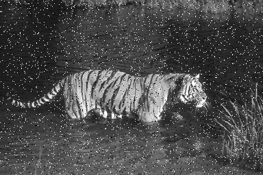
For this reason, this category of filter is also called the edge-preserving filter, and hence, it is highly useful in removing the impulse noise (Fig. 7).
Fig. 7 
Noisy image going through Gaussian and median filter [7]

3 Selection of the Complaisant Filter
Both the filters have a crucial place in the timeline of image processing and both are a preprocessing step. There can be dozens of both types included to create, shape, encounter, and chisel data related to the image. They can be customized to perform in one way under certain conditions and to perform differently when exposed to another set of conditions adhering to the adaptive filter rule generation.
An adaptive filter is a linear filtered system that has a transfer function measured by mutable specifications and a mode to calibrate those parameters as directed by an optimization algorithm. This filter can also work with the nonlinear filter.
The goals of filtering image data fluctuate from noise removal to feature abstraction. Filter construction has mainly two forms: (a) linear and (b) nonlinear. The selection of a relevant filter depends solely on the targets and disposition of the image data that has to be restored.
-
Cases in which the input image data comprises a huge amount of noise but the degree of measure is low, a linear low-pass filter may be adequate.
-
Contrariwise, if an input has a low amount of noise but with a comparably high magnitude, then a nonlinear filter may be more relevant.
-
While linear methods are fast enough, they do not conserve the details of the image, whereas nonlinear filters retain the details well enough.
4 Various Types of Filter
4.1 Mean Filter
It is defined as averaging a linear filter. In this form, filter calculates the mean or average value of all the distorted images in an area which is already pre-decided. Then, the center pixel intensity value is substituted using that mean value. This procedure is performed iteratively on all pixels of the image.
4.2 Median Filter
The median filter is best order statistic and nonlinear filter, whose reciprocation is constructed on the grading of pixel values present in the filter region. In this, the nucleus pixel value is substituted by the intermediate pixel values in the filter vicinity. The median filter performs well for salt-and-pepper noise. The central asset of a median filter is that it can remove input noise with large magnitudes (Fig. 8).

Effect of nonlinear median filter [8]
4.3 Order Statistics Filter
It is a type of nonlinear filter whose riposte is determined by the sequence of pixels covering filtering area. When the nucleus value of the pixel in a picture region is substituted by the 100th percentile, that methodology is termed as max-filter. While on the other hand, if the same pixel value is substituted by the zero percentile, then the filter is considered as the min-filter.
4.4 Adaptive Filter
The behavior of these filters is transmuted based on the demographic traits of the image region, beset by the filter region.
For example, BM3D is sort of adaptive filter. The de-noising algorithm of the adaptive filter can be divided into three steps:
-
1.
Analysis,
-
2.
Processing, and
-
3.
Synthesis.
4.5 Wiener Filter
The Wiener filter intends to eradicate noise which has altered a signal. It follows a statistical approach.

6 Conclusion
-
1.
The achievement of the Wiener filter after performing noise removal for all speckle, Poisson, and Gaussian is of higher quality than mean filter and median filter.
-
2.
The median filter works better for salt-and-pepper noise than mean and Wiener filter.
All the available filters have their specific benefits and disadvantages. One type of filter may work very well with a certain genre of noise but not so good with another kind in the same image. There is a lot of scope for research in this field. Here, we have discussed the various grades of noise that can affect an image during processing and acquisition. Light is thrown on the various ways available to de-noise these images. It can be concluded by saying that using a method that can well preserve the edges of an image is more important than using a method which is fast though the speed factor is equally important. Another technique being used these days is the application of fuzzy systems in filters [10]. Fuzzy logic is related to vagueness and in case of image noise, certain data can be vague [11], [12]; thus, fuzzy systems can work well in this field.
References
https://www.google.co.in/url?sa=i&rct=j&q=&esrc=s&source=images&cd=&cad=rja&uact=8&ved=2ahUKEwjqjfCa-DdAhUJaI8KHY4DB6UQjRx6BAgBEAU&url=https%3A%2F%2Fwww.researchgate.net%2Ffigure%2FImage-03-with-Gaussian-noise-s-5_fig3_291043468&psig=AOvVaw2JU2KcbwyxXoczjILQ4LPG&ust=1536137213527988
http://www.fit.vutbr.cz/~vasicek/imagedb/img_corrupted/impnoise_005/108073.png
https://homepages.inf.ed.ac.uk/rbf/HIPR2/images/fce5noi4.gif
https://www.google.co.in/url?sa=i&rct=j&q=&esrc=s&source=images&cd=&cad=rja&uac=8&ved=2ahUKEwiX1LvFgKHdAhUQTo8KHWW1DMkQjRx6BAgBEAU&url=https%3A%2F%2Fwww.researchgate.net%2Ffigure%2FVisual-results-for-the-Barbara-image-with-JPEG-quantization-noise-Q-7_fig3_220320603&psig=AOvVaw2auKTt5fZpJC20RiwX7082&ust=1536138644050333
Verma R, Ali J (2013) A Comparative study of various types of image noise and efficient noise removal techniques. IJARCSSE, (2277-128X) 3(10)
https://www.google.co.in/url?sa=i&rct=j&q=&esrc=s&source=images&cd=&cad=rja&uact=8&ved=2ahUKEwiQlN3h-DdAhWMq48KHUcCAnsQjRx6BAgBEAU&url=https%3A%2F%2Fwww.giassa.net%2F%3Fpage_id%3D635&psig=AOvVaw2956XMBL6dsaOcTCZD0AEL&ust=1536137338290174
Mehan S, Singla N (2012) Introduction of image restoration using fuzzy filtering. IJARCSS (2277-128X) 2(3)
Mittal A, Goel V (2012) Removal of impulse noise using fuzzy techniques. IJAER (0973-4562) 7(11)
Ville DVD, Nachtegael M, Weken DV, Kerre EE, Philips W, Lamahieu I (2003) Noise reduction by using fuzzy image filtering. IEEE Trans Fuzzy Syst 11(4)
Author information
Authors and Affiliations
Corresponding author
Editor information
Editors and Affiliations
Rights and permissions
Copyright information
© 2019 Springer Nature Singapore Pte Ltd.
About this paper

Cite this paper
Singh, M., Pradhan, S., Islam, M.R., Chitrapriya, N. (2019). A Comparative Study on Different Genres of Image Restoration Techniques. In: Bera, R., Sarkar, S., Singh, O., Saikia, H. (eds) Advances in Communication, Devices and Networking. Lecture Notes in Electrical Engineering, vol 537. Springer, Singapore. https://doi.org/10.1007/978-981-13-3450-4_41
Download citation
DOI: https://doi.org/10.1007/978-981-13-3450-4_41
Published:
Publisher Name: Springer, Singapore
Print ISBN: 978-981-13-3449-8
Online ISBN: 978-981-13-3450-4
eBook Packages: EngineeringEngineering (R0)