RBF-ADRC Based Intelligent Course Control for a Twin Podded Ship

Abstract

Twin podded propulsion is a new type of ship electric propulsion. Equivalent rudder angle analysis method was used to establish a relationship between ship speed and steering angle of POD propeller and the conventional rudder angle, and the maneuverability of twin podded ship was analyzed in different working conditions. RBF-ADRC (active disturbance rejection control) integrated controller is designed for twin podded ship according to its special structure, and the control effect was compared and analyzed with RBF-PID controller through MATLAB.

1 Introduction

Podded electric propulsion ship is different from the conventional ship, because its power and steering is provided by the propulsion motor. Due to the cancellation of the rudder, we can establish a relationship between the speed and steering angle of POD propeller and the conventional rudder angle, namely equivalent rudder angle analysis method.

Mentioned in the literature [1], Ship Manoeuvrability Research and Training Centre (SMRTC) in Poland Get the following conclusion on test of POD type ship: in all cases, POD promote rotary capacity of the ship was very good, the main problems existing is the ability to keep the ship heading stability. The stability of twin podded ship is better than single. So it is very necessary to design the course controller for the problem [2]. Neural network technology is a major bright spot in the field of artificial intelligence, which can achieve a lot of functions and have a successful application in the field of control, becoming a powerful branch of intelligent control. ADRC has strong robustness and wide adaptability, it has the ability to estimate and compensate the uncertain external disturbance, without depending on the mathematical model, it can learn advantages from PID technology and many advanced control technology in process control. The design of the RBF-ADRC course control combines the advantages of both, in order to provide a method for further optimizes the podded ship control problem.

2 The Pod Thrust Vector Model and Equivalent Rudder Angle Analysis Method

2.1 The Pod Thrust Vector Model

The pod thrust vector model can be calculated according to the following formula:

$$\left\{ {\begin{array}{*{20}l} {X_{P} = (1 - t_{p} )(T_{P} \cos \theta_{P} + T_{s} \cos \theta_{s} )} \hfill \\ {Y_{P} = (1 - t_{p} )(T_{P} \sin \theta_{P} + T_{s} \sin \theta_{s} )} \hfill \\ {N_{P} = (1 - t_{p} )(T_{P} \cos \theta_{P} - T_{s} \cos \theta_{s} )0.5{\text{L}}_{PS} + Y_{P} {\text{L}}_{OP} } \hfill \\ \end{array} } \right.$$

(1)

$\theta$ is steering Angle for pods; ${\text{L}}_{PS}$ is the lateral distance between the two propeller; ${\text{L}}_{OP}$ is the distance from the center of the ship to the pods; $T_{P}$ and $T_{s}$ respectively represent left and right pod propeller thrust; $t_{p}$ is the thrust deduction coefficient [3].

$$T_{P} = \rho n_{P}^{2} D^{4} K_{T} (J_{P} )$$

(2)

In formula (2) $\rho$ is for the density of sea water; $n_{P}$ is the left screw rotational speed; D is the propeller diameter; $J_{P} = U_{P} /(n_{P} D)$ is the speed ratio; $K_{T}$ is based on pod propeller open water performance of the map which was used curve fitting and interpolation methods find out the thrust coefficient, the specific formula see (3). $T_{s}$ was calculated in the same way as $T_{P}$.

$$K_{T} = 0.7 + 0.3589J_{P} + 0.1875{{J_{P}}^{2}}$$

(3)

2.2 Equivalent Rudder Angle Analysis Method

Without consideration of the influence of the roll motion of the ship, the force $F_{\delta }$ generated by the conventional rudder is decomposed into the components of the Surge X, the sway Y, and the yaw N [4,5,6], $X_{R}$, $Y_{R}$, $N_{R}$:

$$\left\{ {\begin{array}{*{20}l} {X_{R} = (1 - t_{R} )F_{\delta } \sin \delta } \hfill \\ {Y_{R} = (1 + d_{1R} )F_{\delta } \cos \delta } \hfill \\ {N_{R} = (1 + d_{2R} )x_{G} F_{\delta } \cos \delta } \hfill \\ \end{array} } \right.$$

(4)

In the formula, $F_{\delta } = 0.5\rho {\text{f}}_{a} A_{P} U_{P}^{2} \sin (a_{P} )$, $A_{P}$ is rudder area, U is the flow velocity of rudder blade; ${\text{f}}_{a}$ Is the lift coefficient $C_{L}$ in the slope Angle of attack is equal to zero, $a_{P}$ is angle of attack.

Combined formula (1) and formula (4), this formula can be obtained:

$$\begin{aligned} & 0.5\rho {\text{f}}_{a} A_{P} U_{P}^{2} \sin (a_{P} )(1 + d_{2R} )x_{G} \cos \delta \\ & \quad = (1 - t_{p} )(T_{P} \cos \theta_{P} - T_{s} \cos \theta_{s} )0.5{\text{L}}_{PS} \\ & \quad \quad + \,(1 - t_{p} )(T_{P} \sin \theta_{P} + T_{s} \sin \theta_{s} ){\text{L}}_{OP} \\ \end{aligned}$$

(5)

The formula (2) is brought into the above formula:

$$\begin{aligned} & 0.5\rho {\text{f}}_{a} A_{P} U_{P}^{2} \sin (a_{P} )(1 + d_{2R} )x_{G} \cos \delta \\ & \quad = (1 - t_{p} )(\rho n_{P}^{2} D^{4} K_{T} (J_{P} )\cos \theta_{P} - \rho n_{S}^{2} D^{4} K_{T} (J_{S} )\cos \theta_{s} )0.5{\text{L}}_{PS} \\ & \quad \quad + \,(1 - t_{p} )(\rho n_{P}^{2} D^{4} K_{T} (J_{P} )\sin \theta_{P} + \rho n_{S}^{2} D^{4} K_{T} (J_{S} )\sin \theta_{s} ){\text{L}}_{OP} \\ \end{aligned}$$

(6)

We set $a_{P} { = }\delta$, in the case of the rotation angle is not large, and it can be similar that $\sin a = a,\cos a = 1 - a^{2} /2$, and then the formula can be changed into:

$$\begin{aligned} \delta & = [(1 - t_{p} )(\rho n_{P}^{2} D^{4} K_{T} (J_{P} )(1 - \theta_{P}^{2} /2) \\ & \quad - \,\rho n_{S}^{2} D^{4} K_{T} (J_{S} )(1 - \theta_{S}^{2} /2)0.5{\text{L}}_{PS} \\ & \quad + \,(1 - t_{p} )(\rho n_{P}^{2} D^{4} K_{T} (J_{P} )\theta_{P} \\ & \quad + \,\rho n_{S}^{2} D^{4} K_{T} (J_{S} )\theta_{s} ){\text{L}}_{OP} ]/0.5\rho {\text{f}}_{a} A_{P} U_{P}^{2} (1 + d_{2R} )x_{G} \\ \end{aligned}$$

(7)

We set $(1 - t_{p} )\rho D^{4} /0.5\rho {\text{f}}_{a} A_{P} U_{P}^{2} (1 + d_{2R} )x_{G} = {\text{A}}$, $n_{P}^{2} K_{T} (J_{P} ) = N_{1}$, $n_{S}^{2} K_{T} (J_{S} ) = N_{2}$, The above formula can be simplified as:

$$\begin{aligned} \delta = & {\text{A}}[(N_{1} (1 - \theta_{P}^{2} /2) - N_{2} (1 - \theta_{S}^{2} /2))0.5{\text{L}}_{PS} \\ & \quad + \,(N_{1} \theta_{P} + N_{2} \theta_{s} ){\text{L}}_{OP} ] \\ \end{aligned}$$

(8)

3 Twin Pod of Ship Maneuverability Analysis in Different Working Conditions

In this paper, the simulation is carried out by taking the “Taian port” as an example [7], which used two sets of SSP electric propulsion system. Its main parameters are shown in Table 1.

Table 1 Ship’s main dimensions

According to relevant information, the movement of twin podded ship is divided into the following four conditions [8]:

• (1) The propeller rotation angle is equal, and the rotate speed is same, namely two pods by linkage control. This condition is normal operation in the ocean of the twin podded ship. Applying the equivalent rudder angle method, the given podded propeller rotate speed is 144 r/min, steering angle is 10°, and operate in the MATLAB simulation, we can get the following results (Fig. 1).

  Fig. 1

  

  Equivalent rudder angle and turning circle in first work condition

• (2) Twin podded propellers rotate speed is same, only a single rotary paddle. This condition is ship’s approaching and leaving docks, or correcting the state in special locations. The given left and right POD propeller rotate speed is 144 r/min, the left steering angle is 0°, the right steering angle is 10°, and we can get the following results in MATLAB (Fig. 2).

  Fig. 2

  

  Equivalent rudder and turning circle angle in second work condition

• (3) Single pod function. This condition is when one pod in failure situation. The steering angle and rotate speed of left pod was set zero. The given right podded propeller rotate speed is 144 r/min, and the right steering angle is 10°. The following simulation results can be obtained in MATLAB (Fig. 3).

  Fig. 3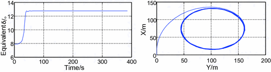

  

  Equivalent rudder angle and turning circle in third work condition

• (4) The twin pods were not turned, but the rotate speeds are different. Because of the particularity of podded propulsion mode, in this case it can still generate torque. It is also well reflect the advanced nature of this propulsion mode. The twin pod steering angle is 0°, given the right podded propeller rotate speed 60 r/min, left the podded propeller rotate speed is 144 r/min. The following simulation results can be obtained in MATLAB (Fig. 4).

  Fig. 4

  

  Equivalent rudder angle and turning circle in fourth work condition

3.1 RBF-ADRC Control Principle

The so-called RBF-ADRC course control is the combination of RBF neural network and auto disturbance rejection controller in the course control. RBF neural network which is a feed-forward neural network is composed of three layers, it is nonlinear structure, but the second hidden layer to the third output layer is linear, so accelerating effectively without the local minimum problem of learning speeds.

The ADRC is mainly composed of tracking differentiator (TD), the nonlinear state error feedback control law (NLSEF) and the expansion of state observer (ESO) three parts [9, 10].

The general steps of the design of RBF-ADRC are summarized as follows:

• (1) By selecting the appropriate parameters, the auto disturbance rejection controller can control the basic course of podded propulsion ship.

• (2) The outputs $z_{1} ,z_{2} ,z_{3}$ were taken from the state observer and save them. The practice of this paper is to import the MATLAB state variable space, in this way to save the data.

• (3) Train the neural network, using RBF neural network, $z_{1} ,z_{2}$ for the input, $z_{3}$ for the expect output. In the course of training, the training parameters and termination conditions are given.

• (4) The trained neural network is embedded into the corresponding position in Fig. 5 in the form of nonlinear function $f_{ANN}$, and then the result of course control is observed.

  Fig. 5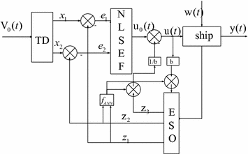

  

  The structure of RBF-ADRC

3.2 Simulation Studies of Course Control

Simulation experiment in this paper using the “Taian port” POD electric propulsion ship as the control object [11, 12]. In order to compare the control effect, the RBF-PID controller [13, 14] as a contrast objects. Target course are 10° and 20°, and initial speed is 15.3 km, ship engine speed 140 r/min.

The simulation curve of course control in the MATLAB is shown below (Figs. 6 and 7).

Fig. 6

Simulation results of RBF-PID course control

Fig. 7

Simulation results of RBF-ADRC course control

When a given course angle is 10°, the RBF-PID controller takes about 200 s to reach a stable value, and has an overshoot about ten percent, while the RBF-ADRC takes only about 70 s. When a given course angle is 20°, the RBF-PID controller takes about 150 s to reach a stable value, while the RBF-ADRC takes only about 60 s. The simulation results show that the two controllers were able to reach the control requirement, but the RBF-ADRC course controller reached the expected course more quickly, and in accordance with the expected steady driving, greatly shorten the adjustment time.

4 Conclusions

This article started with the structure of twin podded propulsion ship, using the equivalent rudder method to study the ship maneuverability and course control problem. the “Taian port” ship was as example to simulate in the MATLAB, mainly completed the following work:

• (1) The thrust vector model of the pod is established, which the mathematical model of ship motion based on.

• (2) By using the method of equivalent rudder effect, the functional relationship between the two twin podded propeller rotate speed, two rotation angle and conventional rudder angle has been established, and four work conditions for ship maneuverability have been analyzed.

• (3) Through the analysis the advantages of RBF neural network and ADRC, the RBF-ADRC course controller has been designed, and compared the control effect with RBF-PID controller, and simulated in the MATLAB. Lay a foundation for further study the control of twin podded ship.

References

Ma C (2007) Podded propulsion technology. Shanghai Jiaotong University Press (in Chinese)
Xian Y, Nie WT (2008) Present situation and prospects of podded rotary electric propulsion systems. Jiangsu Ship 24(6):28–29 (in Chinese)
Gou TT (2012) The research of control system of podded electric propulsion. Jiangsu University of Science and Technology (in Chinese)
Jia XL, Yan YS (1999) Mathematical model of ship motion: the mechanism modeling and ferreting modeling. Dalian Maritime University Press (in Chinese)
Heinke HJ (2004) Investigation about the forces and moments at podded drives. In: Proceedings of the 1st international conference on technological advances in podded propulsion. Newcastle University, UK, April 2004, pp 305–320
Woodward MD, Clarke D, Atlar M () On the manoeuvring prediction of POD driven ship. In: International conference on marine simulation and ship maneuverability (MARSIM 2003), vol 2. Kanazawa, Japan. 25th–28th Aug 2003
Chen XX, Jian D et al (2013) Modeling and simulation of power system for semi submersible ship of Taian (in Chinese)
Huang H, Zhu JX et al (2016) Rotary sculls ship equivalent rudder model. J Harbin Eng Univ (Engl Ed) 37(2):168–173 (in Chinese)
Hui ZG (2009) Semi-submerged ship maneuvering motion simulation. Dalian Maritime University (in Chinese)
Gao Z (2002) From liner to nonlinear contol means: a practical progression. ISA Trans 4(41):177–189 (in Chinese)
Zhang R, Han JQ (2000) A neural network based active disturbance rejection controller. Syst Simul J 12(2):141–151 (in Chinese)
Pan JX (2014) Research on intelligent control for large ship course. Dalian Maritime University (in Chinese)
Xi QC (2014) Research on ship course control based on the ADRC. Dalian Maritime University (in Chinese)
Liu JK (2011) Advanced PID control MATLAB simulation. Electronic Industry Press (in Chinese)
Acknowledgements
The authors are very grateful to the editors and reviewers for their valuable comments and suggestions. This work is supported by National Natural Science Foundation of China (Nos. 51579024, 6137114) and the Fundamental Research Funds for the Central Universities (DMU No. 3132016311).
Author information
Authors and Affiliations
Corresponding author
Editor information
Editors and Affiliations
Rights and permissions
Copyright information
© 2018 Springer Nature Singapore Pte Ltd.
About this paper
Cite this paper
Piao, Z., Guo, C. (2018). RBF-ADRC Based Intelligent Course Control for a Twin Podded Ship. In: Deng, Z. (eds) Proceedings of 2017 Chinese Intelligent Automation Conference. CIAC 2017. Lecture Notes in Electrical Engineering, vol 458. Springer, Singapore. https://doi.org/10.1007/978-981-10-6445-6_48
Download citation
DOI: https://doi.org/10.1007/978-981-10-6445-6_48
Published:
Publisher Name: Springer, Singapore
Print ISBN: 978-981-10-6444-9
Online ISBN: 978-981-10-6445-6
eBook Packages: EngineeringEngineering (R0)