Considerable Analytical Methods

Abstract

The harmonic balance method (HBM) is a technique used in systems including both linear and nonlinear parts. The fundamental idea of HBM is to decompose the system into two separate subsystems, a linear part and a nonlinear part. The linear part is treated in the frequency domain, and the nonlinear part in the time domain. The interface between the subsystems consists of the Fourier transform pair. Harmonic balance is said to be reached when a chosen number of harmonics N satisfy some predefined convergence criteria. First, an appropriate unknown is chosen to use in the convergence check, which is performed in the frequency domain. Then the equations are rewritten in a suitable form for a convergence loop. One starts with an initial value of the chosen unknown, applies the different linear and nonlinear equations, and finally reaches a new value of the chosen unknown. If the difference between the initial value and the final value of the first N harmonics satisfies the predefined convergence criteria, harmonic balance is reached. Otherwise, an increment of the initial value is calculated by using a generalized Euler method—namely, the Newton–Raphson method.

These keywords were added by machine and not by the authors. This process is experimental and the keywords may be updated as the learning algorithm improves.

3.1 Harmonic Balance Method

3.1.1 Introduction

The harmonic balance method (HBM) is a technique used in systems including both linear and nonlinear parts. The fundamental idea of HBM is to decompose the system into two separate subsystems, a linear part and a nonlinear part. The linear part is treated in the frequency domain, and the nonlinear part in the time domain. The interface between the subsystems consists of the Fourier transform pair. Harmonic balance is said to be reached when a chosen number of harmonics N satisfy some predefined convergence criteria. First, an appropriate unknown is chosen to use in the convergence check, which is performed in the frequency domain. Then the equations are rewritten in a suitable form for a convergence loop. One starts with an initial value of the chosen unknown, applies the different linear and nonlinear equations, and finally reaches a new value of the chosen unknown. If the difference between the initial value and the final value of the first N harmonics satisfies the predefined convergence criteria, harmonic balance is reached. Otherwise, an increment of the initial value is calculated by using a generalized Euler method—namely, the Newton–Raphson method.

It should be mentioned that HBM is similar to other proposed coupling techniques, but one advantage of HBM is the calculation of the increment of the initial value. The method proposed by Gupta and Munjal (1992) also includes an iterative process with a convergence condition. The main difference between their method and the HBM is how the chosen convergence unknown is treated. In HBM, one calculates an increment that depends on the difference of the value at the beginning of the convergence loop and the final value after the loop. This implies a faster and more robust convergence. In the method of Gupta and Munjal, the final value is entered as a new initial value, which easily leads to slower convergence or divergence.

For general dynamical systems, the HBM is widely used, from the simplest Duffing oscillation (Liu et al. 2006), to fluid dynamics (Ragulskis et al. 2006), and to complex fluid structural interactions (Liu and Dowell 2005). Wu and Wang (2006) developed Mathematica/Maple programs to approximate the analytical solutions of a nonlinear undamped Duffing oscillation.

For considering this method HBM deals with free vibration of a nonlinear system, having combined the linear and nonlinear springs in series and Nonlinear Normal Modes.

Example 3.1

The conservative oscillation system is formulated as a nonlinear ordinary differential equation having linear and nonlinear stiffness components. The governing equation is linearized and associated with the HBM to establish new and accurate higher-order analytical approximate solutions. Unlike the perturbation method, which is restricted to nonlinear conservative systems with a small perturbed parameter and also unlike the classical HBM which results in a complicated set of algebraic equations, the approach yields simple approximate analytical expressions valid for small as well as large amplitudes of oscillation. Some examples are solved and compared with numerical integration solutions, and the results are published.

3.1.2 Governing Equation of Motion and Formulation

Consider free vibration of a conservative, single-degree-of-freedom system with a mass attached to linear and nonlinear springs in series, as shown in Fig. 3.1. After transformation, the motion is governed by a nonlinear differential equation of motion (see Telli and Kopmaz 2006) as

Fig. 3.1

Nonlinear free vibration of a system of mass with serial linear and nonlinear stiffness on a frictionless contact surface

$$ (1 + 3\varepsilon \,z\,v^{2} )v^{\prime \prime } + 6\varepsilon \,z\,v\,v^{\prime 2} + \omega_{e}^{2} v + \varepsilon \,\omega_{e}^{2} v^{3} = 0, $$

(3.1)

where

$$ \varepsilon = \frac{\beta }{{k_{2} }}, $$

(3.2)

$$ \xi = \frac{{k_{2} }}{{k_{1} }}, $$

(3.3)

$$ z = \frac{\xi }{1 + \xi }, $$

(3.4)

$$ \omega_{e} = \sqrt {\frac{{k_{2} }}{m(1 + \xi )}} $$

(3.5)

with the initial conditions

$$ v(0) = A,\,\,\,\,\,\,v^{\prime } (0) = 0, $$

(3.6)

in which $\varepsilon ,\,\beta ,\,v,\,\omega_{e} ,\,m$, and $\xi$ are perturbation parameter (not restricted to a small parameter), coefficient of nonlinear spring force, deflection of nonlinear spring, natural frequency, mass and the ratio of linear portion $k_{2}$ of the nonlinear spring constant to that of the linear spring constant $k_{1}$, respectively. Note that the notations in Eqs. (3.1)–(3.5) follow those in Telli and Kopmaz (2006). The deflection of linear spring $y_{1} (t)$ and the displacement of attached mass $y_{2} (t)$ can be represented by the deflection of nonlinear spring $v$ in simple relationships as:

$$ y_{1} (t) = \xi \,v(t) + \varepsilon \,\xi \,v(t)^{3} $$

(3.7)

and

$$ y_{2} (t) = v(t) + y_{1} (t). $$

(3.8)

Introducing a new independent temporal variable, $\tau = \omega t$ (Eqs. 3.1 and 3.6), we have

$$ \omega^{2} \left[ {(1 + 3\varepsilon zv^{2} )\ddot{v} + 6\varepsilon zv\dot{v}\,^{2} } \right] + \omega_{e}^{2} v + \varepsilon \,\omega_{e}^{2} v^{3} = 0 $$

(3.9)

and

$$ v(0) = A,\,\,\,\,\,\,\dot{v}(0) = 0, $$

(3.10)

where a dot denotes differentiation with respect to $\tau$. The deflection of nonlinear spring v is a periodic function of $\tau$ with the period of $2\pi$. On the basis of Eq. 3.9, the periodic solution $v(\tau )$ can be expanded in a Fourier series with only odd multiples of $\tau$ as follows:

$$ v(\tau ) = \sum\limits_{n = o}^{\infty } {h_{2n + 1} \cos (2n + 1)\tau .} $$

(3.11)

To linearize the governing differential equation, we assume $v(\tau )$ as the sum of a principal term and a correction term as

$$ v(\tau ) = v_{1} (\tau ) + \Updelta v_{1} (\tau ). $$

(3.12)

Substituting Eq. 3.11 into Eq. 3.9 and neglecting nonlinear terms of $\Updelta v_{1} (\tau )$ yields

$$ \begin{aligned} & \omega^{2} \left[ {\left( {1 + 3\varepsilon zv_{1}^{2} } \right)\ddot{v}_{1} + 6\varepsilon zv_{1} \dot{v}\,_{1}^{2} } \right] + \omega_{e}^{2} v_{1} + \varepsilon \,\omega_{e}^{2} v_{1}^{3} + \left( {\omega_{e}^{2} + 3\varepsilon \,\omega_{e}^{2} v_{1}^{2} } \right)\Updelta v_{1} \\ & + \omega^{2} \left[ {\left( {1 + 3\varepsilon zv_{1}^{2} } \right)\Updelta \ddot{v}_{1} + 2\left( {6\varepsilon zv_{1} \dot{v}_{1} } \right)\Updelta \dot{v}_{1} + \left( {6\varepsilon zv_{1} \ddot{v}_{1} + 6\varepsilon z\dot{v}\,_{1}^{2} } \right)\Updelta v_{1} } \right] = 0, \\ \end{aligned} $$

(3.13)

and

$$ \Updelta v_{1} (0) = 0,\,\,\,\,\,\,\Updelta \dot{v}_{1} (0) = 0, $$

(3.14)

where $v_{1} (\tau ) = A\cos \tau$ is a periodic function of $\tau$ period $2\pi$.

Making use of $v_{1} (\tau ) = A\cos \tau$, we have the following Fourier-series expansions:

$$ \left( {1 + 3\varepsilon zv_{1}^{2} } \right)\ddot{v}_{1} + 6\varepsilon zv_{1} \dot{v}\,_{1}^{2} = \sum\limits_{i = 0}^{\infty } {a_{2i + 1} \cos (2i + 1)\tau } = - \frac{{A(4 + 3A^{2} z\varepsilon )}}{4}\cos \tau - \frac{{9A^{3} z\varepsilon }}{4}\cos 3\tau , $$

(3.15)

$$ \omega_{e}^{2} v_{1} + \varepsilon \,\omega_{e}^{2} v_{1}^{3} = \sum\limits_{i = 0}^{\infty } {b_{2i + 1} \cos (2i + 1)\tau } = \frac{{A\omega_{e}^{2} (4 + 3A^{2} \varepsilon )}}{4}\cos \tau + \frac{{A^{3} \varepsilon \omega_{e}^{2} }}{4}\cos 3\tau , $$

(3.16)

$$ 1 + 3\varepsilon zv_{1}^{2} = \frac{1}{2}c_{0} + \sum\limits_{i = 1}^{\infty } {c_{2i} \cos 2i\tau } = \frac{{2 + 3A^{2} z\varepsilon }}{4} + \frac{{3A^{2} z\varepsilon }}{2}\cos 2\tau , $$

(3.17)

$$ 2(6\varepsilon zv_{1} \dot{v}_{1} ) = \sum\limits_{i = 0}^{\infty } {d_{2(i + 1)} \sin 2(i + 1)\tau } = - 6A^{2} z\varepsilon \sin 2\tau , $$

(3.18)

$$ 6\varepsilon zv_{1} \ddot{v}_{1} + 6\varepsilon z\dot{v}\,_{1}^{2} = \frac{1}{2}c_{0} + \sum\limits_{i = 1}^{\infty } {e_{2i} \cos 2i\tau } = - 6A^{2} \varepsilon \cos 2\tau , $$

(3.19)

$$ \omega_{e}^{2} + 3\varepsilon \,\omega_{e}^{2} v_{1}^{2} = \frac{1}{2}f_{0} + \sum\limits_{i = 1}^{\infty } {f_{2i} \cos 2i\tau } = \frac{{(2 + 3A^{2} \varepsilon )\omega_{e}^{2} }}{2} + \frac{{3A^{2} \varepsilon \omega_{e}^{2} }}{2}\cos 2\tau , $$

(3.20)

where $a_{2i + 1} ,b_{2i + 1} ,c_{2i} ,d_{2(i + 1)} ,e_{2i}$ and $f_{2i} \; {\text{for}}\;i = 0,1,2, \ldots$ are Fourier-series coefficients.

3.1.3 First-Order Analytical Approximation

For the first-order analytical approximation, we set

$$ \Updelta v_{1} (\tau ) = 0, $$

(3.21)

and, therefore,

$$ v(\tau ) = v_{1} (\tau ) = A\cos \tau . $$

(3.22)

Substituting Eqs. 3.15–3.20 into Eq. 3.13, expanding the resulting expression in a trigonometric series and setting the coefficient of $\cos \tau$ to zero yield the solution of the angular frequency $\omega_{1}$, where subscript $\omega_{1}$ indicates the first-order analytical approximation. The analytical approximation of $\omega_{1}$ can be expressed as

$$ \omega_{1} (A) = \omega_{e} \sqrt {\frac{{3\varepsilon A^{2} + 4}}{{3\varepsilon zA^{2} + 4}}} $$

(3.23)

and the periodic solution is

$$ v_{1} (\tau ) = A\cos [\omega_{1} (A)t]. $$

(3.24)

3.1.4 Second-Order Analytical Approximation

For the second analytical approximation, we set

$$ \Updelta v_{1} (\tau ) = x_{1} (\cos \tau - \cos 3\tau ). $$

(3.25)

Substituting Eqs. 3.15–3.20 and 3.25 into Eq. 3.13, expanding the resulting expression in a trigonometric series, and setting the coefficients of $\cos \tau$ and $\cos 3\tau$ to zero result in a quadratic equation of $\omega_{2}^{2}$, where subscript 2 indicates the second-order analytical approximation. The angular frequency $\omega_{2}$ can be expressed as

$$ \omega_{2} (A) = \sqrt {\frac{{ - b - \sqrt {b^{2} - 4ac} }}{2a}} , $$

(3.26)

where

$$ a = - 144A - 252zA^{3} \varepsilon - 135z^{2} A^{5} \varepsilon^{2} , $$

(3.27)

$$ b = 160A\omega_{e}^{2} + 124A^{3} \varepsilon \,\omega_{e}^{2} + 156zA^{3} \varepsilon \,\omega_{e}^{2} + 150zA^{5} \varepsilon^{2} \omega_{e}^{2} , $$

(3.28)

$$ c = - 16A\omega_{e}^{4} - 28A^{3} \varepsilon \,\omega_{e}^{4} - 15A^{5} \varepsilon^{2} \omega_{e}^{4} $$

(3.29)

where $a,b$ and $c$ are the coefficients of the quadratic equation of $\omega_{2}^{2}$. The solution of $\omega_{2}$ in Eq. 3.26 with respect to $+ \sqrt {b^{2} - 4ac}$ is omitted, so that, ${{\omega_{2} } \mathord{\left/ {\vphantom {{\omega_{2} } {\omega_{1} }}} \right. \kern-0pt} {\omega_{1} }} \approx 1$, and the periodic solution is

$$ v_{2} (\tau ) = [A + x_{1} (A)]\cos [\omega_{2} (A)t] - x_{1} (A)\cos [3\omega_{2} (A)t]. $$

(3.30)

where

$$ \begin{aligned} x_{1} (A) = & \, - [32A\omega_{e}^{2} + 25A^{3} \varepsilon \,\omega_{e}^{2} + 15A^{3} z\varepsilon \,\omega_{e}^{2} + 6A^{5} z\varepsilon^{2} \omega_{e}^{2} - (1024A^{2} \omega_{e}^{4} + 1472A^{4} \varepsilon \,\omega_{e}^{4} \\ & + 2112A^{4} z\varepsilon \,\omega_{e}^{4} + 421A^{6} \varepsilon^{2} \omega_{e}^{4} + 365A^{6} z\varepsilon^{2} \omega_{e}^{4} + 981A^{6} z^{2} \varepsilon^{2} \omega_{e}^{4} + 1380A^{8} z\varepsilon^{3} \omega_{e}^{4} \\ & + 1980A^{8} z^{2} \varepsilon^{3} \omega_{e}^{4} + 900A^{10} z^{2} \varepsilon^{4} \omega_{e}^{4} )^{{{1 \mathord{\left/ {\vphantom {1 2}} \right. \kern-0pt} 2}}} ]/[2\omega_{e}^{2} (32 + 51A^{2} \varepsilon + 21A^{2} z\varepsilon + 36A^{4} z\varepsilon^{2} )]. \\ \end{aligned} $$

(3.31)

3.1.5 Third-Order Analytical Approximation

Although the first- and second-order analytical approximations are expected to agree with other solutions, the agreement deteriorates as $t$ progresses during the steady-state response. Therefore, the third-order analytical approximation is derived for a more accurate steady-state response. To construct the third-order analytical approximation, the previous related expressions must be adjusted, due to the interaction between lower-order and higher-order harmonics. Here, $\Updelta v_{1} (\tau )$ and, in Eqs. 3.12, 3.13, and 3.15–3.20, is replaced by $\Updelta v_{2} (\tau )$ and $v_{2} (\tau )$, respectively, and Eq. 3.13 is modified as

$$ \begin{aligned} & \omega^{2} \left[ {\left( {1 + 3\varepsilon zv_{2}^{2} } \right)\ddot{v}_{2} + 6\varepsilon zv_{2} \dot{v}_{2}^{2} } \right] + \omega_{e}^{2} v_{2} + \varepsilon \,\omega_{e}^{2} v_{2}^{3} + \left( {\omega_{e}^{2} + 3\varepsilon \,\omega_{e}^{2} v_{2}^{2} } \right)\Updelta v_{2} \\ & + \omega^{2} \left[ {\left( {1 + 3\varepsilon zv_{2}^{2} } \right)\Updelta \ddot{v}_{2} + 2\left( {6\varepsilon zv_{2} \dot{v}_{2} } \right)\Updelta \dot{v}_{2} + \left( {6\varepsilon zv_{2} \ddot{v}_{2} + 6\varepsilon z\dot{v}_{2}^{2} } \right)\Updelta v_{2} } \right] = 0. \\ \end{aligned} $$

(3.32)

The right-hand sides of Eqs. 3.15–3.20 in the third-order analytical approximation are completely different from the first- and second-order analytical approximations because $v_{1} (\tau )$ is replaced by $v_{2} (\tau )$ of Eq. 3.30. It can be solved directly by substituting the corresponding coefficients of Fourier series in any symbolic software, such as Mathematica.

For the third-order analytical approximation, we set

$$ \Updelta v_{2} (\tau ) = x_{1} (\cos \tau - \cos 3\tau ) + x_{3} (\cos 3\tau - \cos 5\tau ). $$

(3.33)

Substituting the modified Eqs. 3.15–3.20 with $v_{1} (\tau )$ replaced by $v_{2} (\tau )$ and Eq. 3.33 into Eq. 3.32, expanding the resulting expression in a trigonometric series, and setting the coefficients of $\cos \tau ,\cos 3\tau$, and $\cos 5\tau$ to zero yield $\omega_{3}$ as a function of $A$. The corresponding approximate analytical periodic solution can then be solved as

$$ \begin{aligned} v_{3} (\tau ) = & \,[A + x_{1} (A) + x_{2} (A)]\cos [\omega_{3} (A)t] + [x_{3} (A) - x_{2} (A) - x_{1} (A)]\cos [3\omega_{3} (A)t] \\ & - x_{3} (A)\cos [5\omega_{3} (A)t]. \\ \end{aligned} $$

(3.34)

The angular frequency $\omega_{3}$ is the squared-roots of a quadratic equation of $\omega_{3}^{2}$ in the form of

$$ a^{\prime } \left( {\omega_{3}^{2} } \right)^{4}\; + \;b^{\prime }\left( {\omega_{3}^{2} } \right)^{3}\; +\; c^{\prime } \left({\omega_{3}^{2} } \right)^{2}\; +\; d^{\prime } \left({\omega_{3}^{2} } \right) \;+ \;e^{\prime } = 0, $$

(3.35)

where subscript 3 indicates the third-order analytical approximation and $a^{\prime } ,\;b^{\prime } ,\;c^{\prime } ,\;d^{\prime }$, and $e^{\prime}$ are coefficients of the quartic equation of $\omega_{3}^{2}$. There is a total of eight roots, and the particular root which is closest to $\omega_{2}$ is identified as the most appropriate solution because $\omega_{3}$ is a more accurate and of a higher-order approximation to $\omega_{3}$. Comparison of $\omega_{3}$ in the following section shows that it is in excellent agreement with the numerical integration solution for small, as well as large, amplitudes of oscillation. The quartic equation can be subsequently solved by any symbolic software, such as MATHEMATICA, for $\omega_{3}$. The constants $x_{2}$ and $x_{3}$ in Eq. 3.34 derived in terms of the coefficients of Fourier series are obtained.

3.1.6 Approximate Results and Discussion

The solutions of Eq. 3.1 using the second-order LP perturbation method is briefly derived here. Expanding the frequency $\omega^{2} = \omega_{\text{LP}}^{2}$ and the periodic solution $v(\tau ) = v_{\text{LP}} (\tau )$ of Eq. 3.9 into a power series as a function of $\varepsilon$ as follows:

$$ \omega_{\text{LP}}^{2} = \omega_{e}^{2} + \varepsilon \omega_{1} + \varepsilon^{2} \omega_{2} + \cdots $$

(3.36)

$$ v_{\text{LP}} (\tau ) = v_{0} (\tau ) + \varepsilon v_{1} (\tau ) + \varepsilon^{2} v_{2} (\tau ) + \cdots ,\,\,\,\,\,\,\tau = \omega_{\text{LP}} t $$

(3.37)

and setting the coefficients of $\varepsilon^{0} ,\,\varepsilon^{1}$, and $\varepsilon^{2}$ as zero yield

$$ v^{\prime \prime }_{0} + v_{0} = 0,\,\,\,\,\,\,v_{0} (0) = A,\,\,\,\,\,\,v^{\prime }_{0} (0) = 0, $$

(3.38)

$$ v_{1}^{\prime \prime } + v_{1} = - v_{0}^{3} - 6zv_{0} v_{0}^{\prime 2} - 3zv_{0}^{2} v_{0}^{\prime \prime } - \frac{{\omega_{1} v_{0}^{\prime \prime } }}{{\omega_{e}^{2} }},\,\,\,\,\,\,v_{1} (0) = 0,\,\,\,\,\,\,v_{1}^{\prime } (0) = 0, $$

(3.39)

$$ \begin{aligned} v_{2}^{\prime \prime } + v_{2} = & \, - 3v_{0}^{2} v_{1} - 6zv_{1} v_{0}^{\prime 2} - \frac{{6z\omega_{1} v_{0} v_{0}^{\prime 2} }}{{\omega_{e}^{2} }} - 12zv_{0} v^{\prime }_{0} v^{\prime }_{1} - 6zv_{0} v_{1} v_{0}^{\prime \prime } - \frac{{3z\omega_{1} v_{0}^{2} v^{\prime \prime }_{0} }}{{\omega_{e}^{2} }} \\ & - \frac{{\omega_{2} v_{0}^{\prime \prime } }}{{\omega_{e}^{2} }} - 3zv_{0}^{2} v_{1}^{\prime \prime } - \frac{{\omega_{1} v_{1}^{\prime \prime } }}{{\omega_{e}^{2} }},\,\,\,\,\,\,v_{2} (0) = 0,\,\,\,\,\,\,v_{2}^{\prime \prime } (0) = 0. \\ \end{aligned} $$

(3.40)

Solving the linear second-order differential equations 3.38–3.40 with the corresponding initial conditions, we obtain

$$ \omega_{1} = - \frac{3}{4}A^{2} \omega_{e}^{2} (z - 1),\,\,\,\,\,\,\omega_{2} = \frac{3}{128}A^{4} \omega_{e}^{2} (15z^{2} - 14z - 1), $$

(3.41)

$$ \begin{aligned} v_{0} &= \;A\cos \omega_{\text{LP}}t,\,\,\,\,\,\,\,\,\,\,v_{1} = \;\frac{{A^{3} }}{32}(9z - 1)(\cos \omega_{\text{LP}} t - \cos 3\omega_{\text{LP}} t), \\ v_{2} &= - \;\frac{{A^{5} (441z^{2} - 34z - 32)}}{1024}\cos \omega_{\text{LP}} t\;+\; \frac{{3A^{5} (9z^{2} - 1)}}{128}\cos 3\omega_{\text{LP}} t \\ &\quad+\; \frac{{A^{5} (225z^{2} - 34z + 1)}}{1024}\cos 5\omega_{\text{LP}} t. \\ \end{aligned} $$

(3.42)

To further illustrate and verify accuracy of this approximate analytical approach, a comparison of the time history response of nonlinear spring deflection $v(t)$, linear spring deflection $y_{1} (t)$, and mass displacement $y_{2} (t)$ is presented in Figs. 3.2 and 3.3. Figure 3.2 considers the nonlinear hard-spring cases, while Fig. 3.3 represents the nonlinear soft-spring cases.

Fig. 3.2

a Comparison of deflection of nonlinear spring $v(t)$ for various analytical approximations and the numerical integration solution for $m = 1,A = 0.5,\varepsilon = 0.5$, and $\xi = 0.1(k_{1} = 50,k_{2} = 5)$. b Comparison of the deflection of linear spring $y_{1} (t)$ for various analytical approximations and the numerical integration solutions for $m = 1,\varepsilon = 0.5$. c Comparison of the displacement of mass $y_{2} (t)$ for various analytical approximations and the numerical integration solutions for $m = 1,\varepsilon = 0.5$, and $\xi = 0.1\,(k_{1} = 50,k_{2} = 5)$

Fig. 3.3

a Comparison of the deflection of nonlinear spring $v(t)$ for various analytical approximations and the numerical integration solutions for $m = 4,A = 10,\varepsilon = - 0.008$, and $\xi = 0.5(k_{1} = 6,k_{2} = 3)$. b Comparison of the deflection of linear spring $y_{1} (t)$ for various analytical approximations and the numerical integration solutions for $m = 4,\varepsilon = - 0.008$, and $\xi = 0.5(k_{1} = 6,k_{2} = 3)$. c Comparison of the displacement of mass $y_{2} (t)$ for various analytical approximations and the numerical integration solutions for $m = 4,\varepsilon = - 0.008$, and $\xi = 0.5(k_{1} = 6,k_{2} = 3)$

3.2 He’s Parameter Expansion Method

3.2.1 Introduction

Parameter-expanding methods, including the modified Lindstedt–Poincaré method and the bookkeeping parameter method, can successfully deal with such special cases; however, the classical methods fail. The methods need not have a time transformation like the Lindstedt–Poincaré method; the basic character of the method is to expand the solution and some parameters in the equation.

The parameter expansion method is an easy and straightforward approach to nonlinear oscillators. Anyone can apply the method to find an approximation of the amplitude–frequency relationship of a nonlinear oscillator with only basic knowledge of advance calculus. The basic idea of He’s parameter-expanding methods (HPEMs) was provided by Prof. J. H. He in 2002, and the reader is referred to He (2002).

In a case where no parameter exists in an equation, HPEMs can be used (2002). As a general example, the following equation can be considered:

$$ m\,u^{\prime\prime} + \omega_{0}^{2} u + \varepsilon f\,(u,\,u^{\prime},\,u^{\prime\prime}) = 0,\;u(0) = \lambda ,\;u^{\prime}(0) = 0. $$

(3.43)

Various perturbation methods have been applied frequently to analyze Eq. 3.43. The perturbation methods are limited to the case of small ε and $m\,\omega_{0}^{2} > 0$; that is, the associated linear oscillator must be statically stable so that the linear and nonlinear responses are qualitatively similar.

3.2.2 Modified Lindstedt–Poincaré Method

According to the modified Lindstedt–Poincaré method (He 2001b), the solution is expanded into a series of p or ε in the form

$$ u = u_{0} + \varepsilon \,u_{1} + \varepsilon^{2} u_{2} + \cdots $$

(3.44)

Hereby, the parameter ε (or p) does not require being small ($0 \le \varepsilon \le \infty$ or $0 \le p \le \infty$).

The coefficients m and $\omega_{0}^{2}$ are expanded in a similar way

$$ \omega_{0}^{2} = \omega^{2} + \varepsilon \,\omega_{1} + \varepsilon^{2} \omega_{2} + \cdots \quad {\text{or}}\quad \omega_{0}^{2} = \omega^{2} + p\,\omega_{1} + p^{2} \omega_{2} + \cdots $$

(3.45)

$$ m = 1 + \varepsilon \,m_{1} + \varepsilon^{2} m_{2} + \cdots \quad {\text{or}}\quad m = 1 + p\,m_{1} + p^{2} m_{2} + \cdots $$

(3.46)

ω is assumed to be the frequency of the studied nonlinear oscillator; the values for m and $\omega_{0}^{2}$ can be any of these positive, zero, or negative real values.

Here, we are going to solve this problem using HPEM.

3.2.3 Bookkeeping Parameter Method

In this case, no small parameter exists in the equations, so a traditional perturbation method cannot be useful. For this type of problem He introduced a technique in 2001 that provides for a bookkeeping parameter to be entered into the original differential equation (He 2001a).

3.2.4 Application

Example 3.2

This section considers the following nonlinear oscillator with discontinuity (Wang and He 2008):

$$ u^{\prime \prime } + u\left| u \right| = 0,\,\,\,\,\,\,\,\,\,\,u(0) = A,\,\,\,\,\,u^{\prime } (0) = 0. $$

(3.47)

There exists no small parameter in the equation. Therefore, the traditional perturbation methods cannot be applied directly.

The parameter expansion method entails the bookkeeping parameter method and the modified Lindstedt–Poincaré method.

In order to use the HPEM, we rewrite Eq. 3.47 in the form

$$ u^{\prime \prime } + 0.u + 1.u\left| u \right| = 0. $$

(3.48)

According to the parameter expansion method, we may expand the solution, u, the coefficient of u, the zero, and the coefficient of $u\left| u \right|$, 1, in series of $p$:

$$ u = u_{0} + pu_{1} + p^{2} u_{2} + \cdots $$

(3.49)

$$ 0 = \omega^{2} + pa_{1} + p^{2} a_{2} + \cdots $$

(3.50)

$$ 1 = pb_{1} + p^{2} b_{2} + \cdots $$

(3.51)

Substituting Eqs. 3.49 and 3.50 into Eq. 3.48 and equating the terms with the identical powers of $p$, we have

$$ p^{0}{:}u_{0}^{\prime \prime }\; +\; \omega^{2} u_{0} = 0 $$

(3.52)

$$ p^{1}{:}u_{1}^{\prime \prime } \;+\; \omega^{2} u_{1} \;+ \;a_{1} u_{0} \;+ \;b_{1} u_{0} \left| {u_{0} } \right| = 0 $$

(3.53)

$$ p^{2}{:}(1 + \omega^{2} )u_{2}^{\prime \prime } + a_{1} u_{1}^{\prime \prime } + a_{2} u_{0}^{\prime \prime } + b_{1} \left( {\left| {u_{0}^{\prime \prime } } \right|u_{1}^{\prime \prime } + u_{0}^{\prime \prime } \left| {u_{1}^{\prime \prime } } \right|} \right) + b_{2} u_{0}^{\prime \prime } \left| {u_{0}^{\prime \prime } } \right| = 0 . $$

(3.54)

Considering the initial conditions $u_{0} (0) = A$ and $u_{0}^{\prime } (0) = 0$, the solution of Eq. 3.52 is $u_{0} = A\cos \omega t$. Substituting the result into Eq. 3.53, we have

$$ u_{1}^{\prime \prime } + \omega^{2} u_{1} + a_{1} A\cos \omega t + b_{1} A^{2} \cos \omega t\left| {\cos \omega t} \right| = 0. $$

(3.55)

It is possible to perform the Fourier series expansion

$$ \cos \omega t\left| {\cos \omega t} \right| = \sum\limits_{n = 0}^{\infty } {c_{2n + 1} \cos \left[ {(2n + 1)\omega t} \right]} = c_{1} \cos \omega t + c_{3} \cos \omega t + \cdots , $$

(3.56)

where $c_{i}$ can be determined by the Fourier series, for example

$$ c_{1} = \frac{2}{\pi }\int\limits_{0}^{\pi } {\cos^{2} \omega t\left| {\cos \omega t} \right|} \;{\text{d}}(\omega t) = \frac{2}{\pi }\left( {\int\limits_{0}^{{\frac{\pi }{2}}} {\cos^{3} \tau {\text{d}}\tau } - \int\limits_{{\frac{\pi }{2}}}^{\pi } {\cos^{3} \tau {\text{d}}\tau } } \right) = \frac{8}{3\pi }. $$

(3.57)

Substitution of Eq. 3.56 into Eq. 3.55 gives

$$ u_{1}^{\prime \prime } + \omega^{2} u_{1} + \left( {a_{1} + b_{1} A\frac{8}{3\pi }} \right)A\cos \omega t + \sum\limits_{n = 1}^{\infty } {c_{2n + 1} \cos \left[ {(2n + 1)\omega t} \right]} = 0. $$

(3.58)

Not to have a secular term in $u_{1}$ requires that

$$ a_{1} + b_{1} A\frac{8}{3\pi } = 0. $$

(3.59)

If the first-order approximation is enough, then, setting $p = 1$ in Eqs. 3.50 and 3.51, we have

$$ 1 = b_{1} $$

(3.60)

$$ 0 = \omega^{2} + a_{1} . $$

(3.61)

From Eqs. 3.59–3.61, we obtain

$$ \omega = \sqrt {\frac{8A}{3\pi }} \approx 2.6667\sqrt {\frac{A}{\pi }} . $$

(3.62)

The obtained frequency, Eq. 3.62, is valid for the whole solution domain, $0 \;<\; A \;< \;\infty$. The accuracy of frequency can be improved if we continue the solution procedure to a higher order; however, the amplitude obtained by this method is an asymptotic series, not a convergent one. For conservative oscillator

$$ u^{\prime \prime } + f(u)u = 0,\,\,\,\,\,f(u) > 0 $$

(3.63)

where $f(u)$ is a nonlinear function of $u$, we always use the zero-order approximate solution. Thus, we have

$$ u(t) = A\cos \left( {t\sqrt {\frac{8A}{3\pi }} } \right). $$

(3.64)

Example 3.3

3.2.5 Governing Equation

Considering the mechanical system shown in Fig. 3.4, we determine that there is a mass m grounded by linear and nonlinear springs in series. In this figure, the stiffness coefficient of the first linear spring is k ₁; the coefficients associated with the linear and nonlinear portions of spring force in the second spring with cubic nonlinear characteristic are called k ₂ and k ₃, respectively, by definition $\varepsilon$:

Fig. 3.4

Geometry of the example

$$ \varepsilon = \frac{{k_{3} }}{{k_{2} }}, $$

(3.65)

The case of $k_{3} > 0$ corresponds to a hardening spring, while $k_{3} <\; 0$ indicates a softening one. x and y are absolute displacements of the connection point of the two springs and the mass m, respectively. Two new variables have been introduced as follows:

$$ u = y - x,\quad r = x. $$

(3.66)

The following governing equations have been obtained by Telli and Kopmaz (2006):

$$ (1 + 3\varepsilon \,\eta \,u^{2} )\frac{{{\text{d}}^{2} u}}{{{\text{d}}t^{2} }} + 6\,\varepsilon \,\eta \,u\left( {\frac{{{\text{d}}u}}{{{\text{d}}t}}} \right)^{2} \;+\; \omega_{0}^{2} (u + \varepsilon \,u^{3} ) = 0, $$

(3.67)

$$ r = x = \xi \,(1 + \varepsilon \,u^{2} )u,\;y = (1 + \xi + \xi \;\varepsilon \,u^{2} )\,u, $$

(3.68)

$$ \xi = \frac{{k_{2} }}{{k_{1} }},\,\,\,\,\,\eta = \frac{\xi }{1 + \xi },\,\,\,\,\,\omega_{0}^{2} = \frac{{k_{2} }}{m(1 + \xi )}, $$

(3.69)

and the initial conditions are

$$ u(0) = \lambda ,\,\,\,\,\,\frac{{{\text{d}}u}}{{{\text{d}}t}}(0) = 0. $$

(3.70)

3.2.6 HPEM for Solving Problem

According to the HPEM, Eq. 3.67 can be rewritten as (Kimiaeifar et al. 2010):

$$ \frac{{{\text{d}}^{2} u}}{{{\text{d}}t^{2} }} + \omega_{0}^{2} u + \varepsilon \left( {3\eta \,u^{2} \frac{{{\text{d}}^{2} u}}{{{\text{d}}t^{2} }} + 6\,\eta \,u\left( {\frac{{{\text{d}}u}}{{{\text{d}}t}}} \right)^{2} + \omega_{0}^{2} u^{3} } \right) = 0. $$

(3.71)

And initial conditions are

$$ u(0) = \lambda ,\;\frac{{{\text{d}}u}}{{{\text{d}}t}}(0) = 0. $$

(3.72)

The form of solution and the constant one in Eq. 3.71 can be expanded as

$$ u(t) = u_{0} (t) + \varepsilon \,u_{1} (t) + \varepsilon^{2} u_{2} (t) + \cdots $$

(3.73)

$$ \omega_{0}^{2} = \omega^{2} + \varepsilon \,b_{1} + \varepsilon^{2} b_{2} + \cdots $$

(3.74)

Substituting Eqs. 3.72–3.74 into Eq. 3.71 and processing as the standard perturbation method, we have

$$ \frac{{{\text{d}}^{2} u_{0}}}{{{\text{d}}t^{2} }} + \omega^{2}{u_{0}} = 0,\;\quad{u_{0}}(0) = \lambda ,\;\quad\frac{{\text{d}}u_{0}}{{\text{d}}t}(0) = 0. $$

(3.75)

The solution of Eq. 3.75 is

$$ u_{0} (t) = \lambda \cos (\omega \,t). $$

(3.76)

Substituting x ₀(t) from the above equation into Eq. 3.76 results in

$$ \begin{aligned} & \frac{{{\text{d}}^{2} u_{1} (t)}}{{{\text{d}}t^{2} }} + \omega^{2} u_{1} (t) + b_{1} \lambda \cos (\omega \,t) - 3\eta \lambda^{3} \cos^{3} (\omega \,t)\omega^{2} + \omega_{0}^{2} \lambda^{3} \cos^{3} (\omega \,t) \\ &\quad + 6\eta \lambda^{3} \cos (\omega \,t)\sin^{2} (\omega \,t)\omega^{2} = 0. \\ \end{aligned} $$

(3.77)

But considering Eq. 3.74 and assuming two first terms, we have

$$ b_{1} = \frac{{\omega_{0}^{2} - \omega^{2} }}{\varepsilon }. $$

(3.78)

On the basis of trigonometric functions properties, we have

$$ \cos^{3} (\omega \,t) = 1/4\cos (3\omega \,t) + 3/4\cos (\omega \,t). $$

(3.79)

Substituting Eq. 3.79 into Eq. 3.77 and eliminating the secular term leads to

$$ b_{1} \lambda + \frac{3}{4}\omega_{0}^{2} \lambda^{3} k\, - \frac{3}{4}\eta \lambda^{3} \omega^{2} = 0. $$

(3.80)

Substituting Eq. 3.79 into Eq. 3.80, two roots of this particular equation can be obtained as

$$ \omega = \pm \frac{{\omega_{0} \sqrt {(3\eta \lambda^{2} \varepsilon + 4)(4 + 3\lambda^{2} \varepsilon )} }}{{3\eta \lambda^{2} \varepsilon + 4}}. $$

(3.81)

Replacing ω from Eq. 3.81 into Eq. 3.77 yields

$$ u(t) = u_{0} (t) = \lambda \cos \left( {\frac{{\omega_{0} \sqrt {(3\eta \lambda^{2} \varepsilon + 4)(4 + 3\lambda^{2} \varepsilon )} }}{{3\eta \lambda^{2} \varepsilon + 4}}\,t} \right). $$

(3.82)

3.3 Differential Transformation Method

3.3.1 Introduction

The differential transform method (DTM) is an analytic method for solving differential equations. The concept of a differential transform was first introduced by Zhou in 1986. Its main application therein is to solve both linear and nonlinear initial value problems in electric circuit analysis. This method constructs an analytical solution in the form of a polynomial. It is different from the traditional higher order Taylor series method. The Taylor series method is computationally expensive for large orders. The DTM is an alternative procedure for obtaining an analytic Taylor series solution of the differential equations. By using DTM, we get a series solution—in practice, a truncated series solution. The series often coincides with the Taylor expansion of the true solution at point x = 0, in the initial value case.

Such a procedure changes the actual problem to make it tractable by conventional methods. In short, the physical problem is transformed into a purely mathematical one for which a solution is readily available. Our concern in this work is the derivation of approximate analytical oscillatory solutions for the nonlinear oscillator equation (Hassan 2002; Momani 2008):

$$ y^{\prime \prime } (t) + cy(t) = \varepsilon f(y(t),y^{\prime } (t)),\,\,\,\,\,\,\,\,\,\,y(0) = a,\,\,\,\,\,y^{\prime } (0) = b, $$

(3.83)

where $c$ is a positive real number and $\varepsilon$ is a parameter (not necessarily small). We assume that the function $f(y(t),y^{\prime } (t))$ is an arbitrary nonlinear function of its arguments. The modified DTM will be employed in a straightforward manner without any need for linearization or smallness assumptions.

3.3.2 Differential Transformation Method

This technique, the given differential equation, and related boundary conditions are transformed into a recurrence equation that finally leads to the solution of a system of algebraic equations as coefficients of a power series. This method is useful for obtaining exact and approximate solutions of linear and nonlinear differential equations. There is no need for linearization or perturbations; large computational work and round-off errors are avoided. It has been used to solve effectively, easily, and accurately a large class of linear and nonlinear problems with approximations. The method is well addressed in Ayaz (2004), Hassan (2004) and Liu and Song (2007). The basic definitions of differential transformation are introduced as follows:

Definition 3.1

If $f(t)$ is analytic in the time domain $T$, then it will be differentiated continuously with respect to time t:

$$ \phi (t,k) = \frac{{{\text{d}}^{k} f(t)}}{{{\text{d}}t^{k} }},\,\,\,\,\,\,\,\,\,\,\forall_{t} \in T. $$

(3.84)

For $t = t_{i}$, $\phi (t,k) = \phi (t_{i} ,k)$, where $k$ belongs to the set of nonnegative integers, denoted as the K-domain. Therefore, Eq. 3.84 can be rewritten as

$$ F(k) = \phi (t_{i} ,k) = \left. {\left[ {\frac{{{\text{d}}^{k} f(t)}}{{{\text{d}}t^{k} }}} \right]} \right|_{{t = t_{i} }} ,\,\,\,\,\,\,\,\,\,\,\forall_{t} \in K, $$

(3.85)

where $F(k)$ is called the spectrum of $f(t)$ at $t = t_{i}$ in the K-domain.

Definition 3.2

If $f(t)$ can be represented by the Taylor series, then it can be indicated as

$$ f(t) = \sum\limits_{k = 0}^{\infty } {\left[ {{{(t - t_{i} )^{k} } \mathord{\left/ {\vphantom {{(t - t_{i} )^{k} } {k!}}} \right. \kern-0pt} {k!}}} \right]} \,F(k). $$

(3.86)

Equation 3.86 is called the inverse transform of $F(k)$. With the symbol $D$ denoting the differential transformation process, and upon combining Eqs. 3.85 and 3.86, we obtain

$$ f(t) = \sum\limits_{k = 0}^{\infty } {\left[ {{{(t - t_{i} )^{k} } \mathord{\left/ {\vphantom {{(t - t_{i} )^{k} } {k!}}} \right. \kern-0pt} {k!}}} \right]} \,F(k) \equiv D^{ - 1} F(k). $$

Using the differential transformation, a differential equation in the domain of interest can be transformed into an algebraic equation in the K-domain, and $f(t)$ can be obtained by the finite–term Taylor series expansion plus a remainder such as

$$ f(t) = \sum\limits_{k = 0}^{N} {\left[ {{{(t - t_{i} )^{k} } \mathord{\left/ {\vphantom {{(t - t_{i} )^{k} } {k!}}} \right. \kern-0pt} {k!}}} \right]} \,F(k) + R_{N + 1} (t). $$

The fundamental mathematical operations performed by DTM are listed in Table 3.1.

Table 3.1 The fundamental operations of the differential transform method

In addition to the above operations, the following theorem, which can be deduced from Eqs. 3.85 and 3.86, is given below:

Theorem 3.1

If $f(x) = g_{1} (x)g_{2} (x) \cdots g_{m - 1} (x)g_{m} (x)$, then

$$\begin{aligned}F(k) &= \sum\limits_{{k_{n - 1} = 0}}^{k} {\sum\limits_{{k_{n - 2} = 0}}^{{k_{n - 1} }} { \ldots \sum\limits_{{k_{2} = 0}}^{{k_{3} }} {\sum\limits_{{k_{1} = 0}}^{{k_{2} }} {G_{1} (k_{1} )G_{2} (k_{2} - k_{1} ) \cdots } } } } G_{n - 1} (k_{n - 1} - k_{n - 2} ) \\ &\quad G_{n} (k - k_{n - 1} ).\end{aligned}$$

(3.87)

The series solution (3.8) does not exhibit the periodic behavior that is characteristic of oscillator equations. It converges rapidly only in a small region; in the wide region, they may have very slow convergence rates, and then their truncations yield inaccurate results. In the modified DTM of Shaher Momani, we apply a Laplace transform to the series obtained by DTM, then convert the transformed series into a meromorphic function by forming its Padé approximants, and then invert the approximant to obtain an analytic solution, which may be periodic or a better approximation solution than the DTM truncated series solution (Momani 2008).

3.3.3 Padé Approximations

A Padé approximant is the ratio of two polynomials constructed from the coefficients of the Taylor’s series expansion of a function $y(x)$. The $\left[ {{L \mathord{\left/ {\vphantom {L M}} \right. \kern-0pt} M}} \right]$ Padé approximations of a function $y(x)$ are given by Baker in 1975 as

$$ \left[ {{L \mathord{\left/ {\vphantom {L M}} \right. \kern-0pt} M}} \right] = \frac{{P_{L} (x)}}{{Q_{M} (x)}}. $$

(3.88)

where $P_{L} (x)$ is a polynomial of degree at most $L$ and $Q_{M} (x)$ is a polynomial of degree at most $M$. The formal power series are

$$ y(x) = \sum\limits_{i = 1}^{\infty } {a_{i} x^{i} ,} $$

(3.89)

$$ y(x) - \frac{{P_{L} (x)}}{{Q_{M} (x)}} \;=\; O(x^{L + M + 1} ), $$

(3.90)

which determine the coefficients of $P_{L} (x)$ and $Q_{M} (x)$ by the equation.Since we can clearly multiply the numerator and denominator by a constant and leave $\left[ {{L \mathord{\left/ {\vphantom {L M}} \right. \kern-0pt} M}} \right]$ unchanged, we impose the normalization condition

$$ Q_{M} (0) = 1.0. $$

(3.91)

Finally, we require that $P_{L} (x)$ and $Q_{M} (x)$ have no common factors. If we write the coefficient of $P_{L} (x)$ and $Q_{M} (x)$ as

$$ \left. \begin{aligned} P_{L} (x) & = p_{0} + p_{1} x + p_{2} x^{2} + \cdots P_{L} x^{L} \\ Q_{M} (x) & = q_{0} + q_{1} x + q_{2} x^{2} + \cdots q_{M} x^{M} \\ \end{aligned} \right\}. $$

(3.92)

then, by Eqs. 3.91 and 3.92, we may multiply Eq. 3.90 by $Q_{M} (x)$, which linearizes the coefficient equations. We can write out Eq. 3.90 in more detail as

$$ \left. \begin{aligned} & a_{L + 1} + a_{L} q_{1} + \cdots a_{L - M + 1} q_{M} = 0, \\ & a_{L + 2} + a_{L + 1} q_{1} + \cdots a_{L - M + 2} q_{M} = 0, \\ & \vdots \\ & a_{L + M} + a_{L + M - 1} q_{1} + \cdots a_{L} q_{M} = 0, \\ \end{aligned} \right\} $$

(3.93)

$$ \left. \begin{aligned} & a_{o} = p_{0} , \\ & a_{0} + a_{0} q_{1} = p_{1} , \\ & a_{2} + a_{1} q_{1} + a_{0} q_{2} = p_{1} , \\ & \vdots \\ & a_{L} + a_{L - 1} q_{1} + \cdots + a_{0} q_{L} = p_{L} \\ \end{aligned} \right\}. $$

(3.94)

To solve these equations, we start with Eq. 3.93, which is a set of linear equations for all unknown $q$s. Once the $q$s are known, Eq. 3.94 gives an explicit formula for the unknown $p$s, which completes the solution. If Eqs. 3.93 and 3.94 are nonsingular, then we can solve them directly and obtain Eq. 3.95 (Baker 1975), where Eq. 3.95 holds, and if the lower index on a sum exceeds the upper, the sum is replaced by zero:

$$ \left[ \frac{L}{M} \right] = \frac{{\det \left[ {\begin{array}{*{20}c} {a_{L - M + 1} } & {a_{L - M + 2} } & \ldots & {a_{L + 1} } \\ \vdots & \vdots & \ddots & \vdots \\ {a_{L} } & {a_{L + 1} } & \ldots & {a_{L + M} } \\ {\sum\nolimits_{j = M}^{L} {a_{j - M} x^{j} } } & {\sum\nolimits_{j = M - 1}^{L} {a_{j - M + 1} x^{j} } } & \ldots & {\sum\nolimits_{j = 0}^{L} {a_{j} x^{j} } } \\ \end{array} } \right]}}{{\det \left[ {\begin{array}{*{20}c} {a_{L - M + 1} } & {a_{L - M + 2} } & \ldots & {a_{L + 1} } \\ \vdots & \vdots & \ddots & {} \\ {a_{L} } & {a_{L + 1} } & \ldots & {a_{L + M} } \\ {x^{M} } & {x^{M - 1} } & \ldots & 1 \\ \end{array} } \right]}}. $$

(3.95)

To obtain diagonal Padé approximants of different order, such as [2/2], [4/4], or [6/6], we can use the symbolic calculus software, MATHEMATICA.

3.3.4 Application

Example 3.4

In this example, the DTM is used to solve subharmonic resonances of nonlinear oscillation systems with parametric excitations, governed by Hassan (2002)

$$ \frac{{{\text{d}}^{2} x(t)}}{{{\text{d}}t^{2} }} + (1 - \varepsilon \cos (\phi t))(\lambda x(t) + \beta x(t)^{3} ) = 0\quad x(0) = A,\;\dot{x}(0) = 0, $$

(3.96)

where $\varepsilon ,\phi ,\beta ,\lambda$ are known as physical parameters.

A comparison of the present results with those yielded by the established Runge–Kutta method confirms the accuracy of the proposed method.

Applying the DTM to Eq. 3.96 with respect to $t$ gives (Hassan 2002)

$$ \begin{aligned} & (k + 2)(k + 1)X_{k + 2} + \lambda X_{k} - \lambda \varepsilon \left( {\sum\limits_{l = 0}^{k} {\frac{{X_{k - l} \phi^{l} \cos \left( {\frac{1}{2}\pi l} \right)}}{l!}} } \right) + \beta \left( {\sum\limits_{l = 0}^{k} {X_{k - l} \left( {\sum\limits_{p = 0}^{l} {X_{l - p} X_{p} } } \right)} } \right) \\ & - \beta \varepsilon {\left( {\sum\limits_{l = 0}^{k} {\frac{1}{(k - l)!}\left( {\phi^{(k - l)} \cos \left( {\frac{1}{2}(k - l)\pi } \right)} \right)\left( {\sum\limits_{p = 0}^{l} {X_{l - p} \left( {\sum\limits_{q = 0}^{p} {X_{p - q} X_{q} } } \right)} } \right)} } \right)} = 0. \\ \end{aligned} $$

(3.97)

Suppose that $X_{0}$ and $X_{1}$ are apparent from boundary conditions. By solving Eq. 3.97 with respect to $X_{k + 2}$, we will have

$$ X_{2} = \frac{1}{2}\beta \varepsilon X_{0}^{3} - \frac{1}{2}\lambda X_{0} + \frac{1}{2}\lambda \varepsilon X_{0} - \frac{1}{2}\beta X_{0}^{3} , $$

(3.98)

$$ \begin{aligned} X_{3} = & \, - \frac{1}{6}\lambda X_{1} + \frac{1}{6}\lambda \varepsilon X_{1} + \frac{1}{6}\lambda \varepsilon X_{0} \phi \cos \left( {\frac{1}{2}\pi } \right), \\ & - \frac{1}{2}\beta X_{1} X_{0}^{2} + \frac{1}{6}\beta \varepsilon \phi \cos \left( {\frac{1}{2}\pi } \right)X_{0}^{3} + \frac{1}{2}\beta \varepsilon X_{1} X_{0}^{2} , \\ \end{aligned} $$

(3.99)

$$ \begin{aligned} X_{4} = & \, - \frac{1}{3}\lambda \beta \varepsilon X_{0}^{3} + \frac{1}{24}\lambda^{2} X_{0} - \frac{1}{12}\lambda^{2} \varepsilon X_{0} + \frac{1}{6}\lambda \beta X_{0}^{3} \\ & + \frac{1}{6}\lambda \beta \varepsilon^{2} X_{0}^{3} + \frac{1}{24}\lambda^{2} \varepsilon^{2} X_{0} + \frac{1}{12}\lambda \varepsilon X_{1} \phi \cos \left( {\frac{1}{2}\pi } \right) + \cdots \\ \end{aligned} $$

(3.100)

$$ \begin{aligned} X_{5} = & \,\frac{1}{20}\beta \varepsilon X_{1}^{3} + \frac{9}{40}X_{0}^{4} \beta^{2} X_{1} + \frac{1}{120}\lambda^{2} \varepsilon^{2} X_{1} - \frac{1}{60}\lambda^{2} \varepsilon X_{1} - \frac{1}{30}\lambda^{2} \varepsilon X_{0} \phi \cos \left( {\frac{1}{2}\pi } \right) \\ & + \frac{1}{120}\lambda^{2} X_{1} + \frac{1}{120}\lambda \varepsilon X_{0} \phi^{3} \cos \left( {\frac{3}{2}\pi } \right) + \frac{1}{40}\lambda \varepsilon X_{1} \phi^{2} \cos (\pi ) + \cdots \\ \end{aligned} $$

(3.101)

The above process is continuous. Substituting Eqs. 3.98–3.101 into the main equation on the basis of DTM, the closed form of the solutions can be obtained:

$$ \begin{aligned} x(t) = & \,X_{0} + tX_{1} + \frac{{t^{2} }}{2!}\left( {\frac{1}{2}\beta \varepsilon X_{0}^{3} - \frac{1}{2}\lambda X_{0} + \frac{1}{2}\lambda \varepsilon X_{0} - \frac{1}{2}\beta X_{0}^{3} } \right) \\ & + \frac{{t^{3} }}{3!}\left( { - \frac{1}{6}\lambda X_{1} + \frac{1}{6}\lambda \varepsilon X_{1} + \frac{1}{6}\lambda \varepsilon X_{0} \phi \cos \left( {\frac{1}{2}\pi } \right) - \frac{1}{2}\beta X_{1} X_{0}^{2} + \frac{1}{6}\beta \varepsilon \phi \cos (\frac{1}{2}\pi )X_{0}^{3} + \frac{1}{2}\beta \varepsilon X_{1} X_{0}^{2} } \right) + \cdots \\ \end{aligned} $$

(3.102)

In this stage, in order to achieve higher accuracy, we use a subdomain technique; that is, the domain of $t$ should be divided into some adequate intervals. The values at the end of each interval will be the initial values of the next one. For example, at the first subdomain, it is assumed that the distance of each interval is 0.2. For the first interval, $0 \to 0.2$, boundary conditions are the ones given in Eq. 3.96 at point $t = 0$. By exerting a transformation, we will have

$$ X_{0} = A. $$

(3.103)

And the other boundary conditions are considered as

$$ X_{1} = 0. $$

(3.104)

As was mentioned above, for the next interval, $0.2 \to 0.4$, new boundary conditions are

$$ X_{0} = x(0.2). $$

(3.105)

The next boundary condition is considered as

$$ X_{ 1} = \frac{{{\text{d}}x}}{{{\text{d}}t}}(0.2). $$

(3.106)

For this interval function, $x(t)$ is represented by power series whose center is located at $0.2$, which means that in this power series $t$ converts to$(t - 0.2)$.

In order to verify the effectiveness of the proposed DTM, by using the Maple 10, package, the fourth-order Runge–Kutta as a numerical method is used to compute the displacement response of the nonlinear oscillator for a set of initial amplitudes and different physical parameters. These results are then compared with the DTM corresponding to the same set of amplitudes.

The results for the different methods of DTM and Runge–Kutta are compared in Fig. 3.5.

Fig. 3.5

The comparison between the differential transformation method (DTM) and numerical solutions (NS) of $x[m]$ to $t[s]$, for a A = 3, λ = 3, β = 2, $\varepsilon = 0.01,\phi = 10$ and b A = 4, λ = 2, β = 2, $\varepsilon = 0.01,\,\,\phi = 10$

Example 3.5

In order to assess the advantages and the accuracy of the modified DTM for solving nonlinear oscillatory systems, we have applied the method to a variety of initial-value problems arising in nonlinear dynamics. All the results are calculated by using Mathematica.

Consider the Van der Pol equation,

$$ y^{\prime \prime } (t) + y(t) = \varepsilon \left[ {1 - y^{2} (t)} \right]y^{\prime } (t),\,\,\,\,\,\,\,\,\,\,y(0) = 0,\,\,\,\,\,y^{\prime } (0) = 2, $$

(3.107)

With respect to the initial conditions, we have

$$ y(0) = 0,\,\,\,\,\,y^{\prime } (0) = 2. $$

(3.108)

Taking the differential transform of both sides of Eq. 3.107, we obtain the recurrence relation

$$ \begin{aligned} Y(k + 2) = & \,\frac{1}{(k + 1)(k + 2)} \\ & \times \left[ {\varepsilon \left( {(k + 1)Y(k + 2) - \sum\limits_{{k_{2} = 0}}^{k} {\sum\limits_{{k_{1} = 0}}^{{k_{2} }} {(k - k_{2} + 1)Y(k_{1} )Y(k_{2} - k_{1} )Y(k - k_{2} + 1)} } } \right) - Y(k)} \right]. \\ \end{aligned} $$

(3.109)

The initial conditions given in Eq. 3.109 can be transformed at $t_{0} = 0$ as

$$ Y(0) = 0,\,\,\,\,\,Y(1) = 2. $$

(3.110)

By using Eqs. 3.109, 3.110, and 3.107, the solution of the following series is obtained:

$$ y(t) = 2\left( {t - \frac{{t^{3} }}{3!} + \frac{{t^{5} }}{5!} - \frac{{t^{7} }}{7!}} \right) + \varepsilon \left( {t^{2} - \frac{{5t^{4} }}{6} + \frac{{91t^{6} }}{360} - \frac{{41t^{8} }}{1008}} \right) + \cdots $$

(3.111)

This series does not exhibit the periodic behavior that is characteristic of the oscillatory system (3.107 and 3.108). Comparison of the approximate solution (3.111) for $\varepsilon = 0.3$ and the solution obtained by the fourth-order Runge–Kutta method in Fig. 3.6 shows that it converges in a small region but yields a wrong solution in a wider region. In order to improve the accuracy of the differential transform solution (3.111), we implement the modified DTM as follows.

Fig. 3.6

Plots of displacement y versus time t: Runge–Kutta method, (—); Eq. 3.8, (– –)

Applying the Laplace transform to the series solution (3.111), yields

$$ L\left[ {y(t)} \right] = 2\left( {\frac{1}{{s^{2} }} - \frac{1}{{s^{4} }} + \frac{1}{{s^{6} }} - \frac{1}{{s^{8} }}} \right) + \varepsilon \left( {\frac{2}{{s^{3} }} - \frac{20}{{s^{5} }} + \frac{182}{{s^{7} }} - \frac{1640}{{s^{9} }}} \right) + \cdots $$

(3.112)

For simplicity, let $s = {1 \mathord{\left/ {\vphantom {1 t}} \right. \kern-0pt} t}$; then

$$ L\left[ {y(t)} \right] = 2\left( {t^{2} - t^{4} + t^{6} - t^{8} } \right) + \varepsilon \left( {2t^{3} - 20t^{5} + 182t^{7} - 1640t^{9} } \right) + \cdots $$

(3.113)

The [4/4] Padé approximation for the terms containing $\varepsilon^{0} ,\;\varepsilon^{1} , \ldots$ separately gives

$$ \left[ \frac{4}{4} \right] = 2\left( {\frac{{t^{2} }}{{1 + t^{2} }}} \right) + \varepsilon \left( {\frac{{2t^{3} }}{{1 + 10t^{2} + 9t^{4} }}} \right). $$

Recalling $t = {1 \mathord{\left/ {\vphantom {1 s}} \right. \kern-0pt} s}$, we obtain [4/4] in terms of $s$ as

$$ \left[ \frac{4}{4} \right] = 2\left( {\frac{1}{{s^{2} + 1}}} \right) + \varepsilon \left( {\frac{2s}{{s^{4} + 10s^{2} + 9}}} \right). $$

By using the inverse Laplace transform to the [4/4] Padé approximation, we obtain the modified approximate solution

$$ y(t) = 2\sin (t) + \varepsilon \cos (t)\sin^{2} (t). $$

(3.114)

3.4 Adomian’s Decomposition Method

3.4.1 Basic Idea of Adomian’s Decomposition Method

The Adomian decomposition method (ADM) is a nonnumerical method for solving nonlinear differential equations, both ordinary and partial. The general direction of this work is toward a unified theory for partial differential equations (PDEs). The method was developed by George Adomian, chair of the Center for Applied Mathematics at the University of Georgia, in 1984. This method is a semianalytical method.

The ADM had been represented by Adomian (1994a, b, 1992). This method is a semianalytical method and has been modified by Wazwaz (1999a, b, 2001) and, more recently, by Luo (2005) and Zhang et al. (2006). This method is useful for obtaining closed form or numerical approximation for a wide class of stochastic and deterministic problems in science and engineering. These problems involve algebraic, linear or nonlinear ordinary or partial differential equations, and integro-differential, integral, and differential delay equations.

Let us discuss a brief outline of the ADM. For this, we consider a general nonlinear equation in the form

$$ Lu + Ru + Nu = g $$

(3.115)

where $L$ is the highest order derivative that is assumed to be easily invertible, $R$ is the linear differential operator of less order than $L$, $Nu$ presents the nonlinear terms, and $g$ is the source term. Applying the inverse operator $L^{ - 1}$ to both sides of Eq. 3.115 and using the given conditions, we obtain

$$ u = f\left( x \right) - L^{ - 1} \left( {Ru} \right) - L^{ - 1} \left( {Nu} \right) $$

(3.116)

where the function $f\left( x \right)$ represents the terms arising from integration of the source term $g\left( x \right)$, using given conditions. For nonlinear differential equations, the nonlinear operator $Nu = F\left( u \right)$ is represented by an infinite series of the so-called Adomian polynomials as

$$ F\left( u \right) = \sum\limits_{m = 0}^{\infty } {A_{m} } . $$

(3.117)

The polynomials $A_{m}$ are generated for all kinds of nonlinearity so that $A_{0}$ depends only on $u_{0}$, $A_{1}$depends on $u_{0}$ and $u_{1}$, and so on. The Adomian polynomials introduced above show that the sum of subscripts of the components of $u$ for each term of $A_{m}$ is equal to $n$.

The Adomian method defines the solution $u\left( x \right)$ by the series

$$ u = \sum\limits_{m = 0}^{\infty } {u_{m} } . $$

(3.118)

In the case of $F\left( u \right)$, the infinite series is a Taylor expansion about $u_{0}$,

$$ F\left( u \right) = F\left( {u_{0} } \right) + F^{\prime } \left( {u_{0} } \right)\left( {u - u_{0} } \right) + F^{\prime \prime } \left( {u_{0} } \right)\frac{{\left( {u - u_{0} } \right)}}{2!} + F^{\prime \prime \prime } \left( {u_{0} } \right)\frac{{\left( {u - u_{0} } \right)^{2} }}{3!} + \cdot \cdot \cdot $$

(3.119)

Rewriting Eq. 3.118 as $u - u_{0} = u_{1} + u_{2} + u_{3} + \cdots$, substituting it into Eq. 3.119, and then equating two expressions for $F\left( u \right)$ found in Eqs. 3.119 and 3.117 define formulas for the Adomian polynomials in the form of

$$ F\left( u \right) = A_{1} + A_{2} + \cdots = F\left( {u_{0} } \right) + F^{\prime} \left( {u_{0} } \right)\left( {u_{1} + u_{2} + \cdots } \right) + F^{\prime \prime} \left( {u_{0} } \right)\frac{{\left( {u_{1} + u_{2} + \cdots } \right)^{2} }}{2!} + \cdots $$

(3.120)

By equating terms in Eq. 3.120, the first few Adomian’s polynomials $A_{0} ,$ $A_{1} ,$ $A_{2} ,$ $A_{3}$, and $A_{4}$ are given by:

$$ A_{0} = F\left( {u_{0} } \right), $$

(3.121)

$$ A_{1} = u_{1} F^{\prime } \left( {u_{0} } \right), $$

(3.122)

$$ A_{2} = u_{2} F^{\prime } \left( {u_{0} } \right) + \frac{1}{2!}u_{1}^{2} F^{\prime \prime } \left( {u_{0} } \right), $$

(3.123)

$$ A_{3} = u_{3} F^{\prime } \left( {u_{0} } \right) + u_{1} u_{2} F^{\prime \prime } \left( {u_{0} } \right) + \frac{1}{3!}u_{1}^{3} F^{\prime \prime \prime } \left( {u_{0} } \right), $$

(3.124)

$$ A_{4} = u_{4} F^{\prime } \left( {u_{0} } \right) + \left( {\frac{1}{2!}u_{2}^{2} + u_{1} u_{3} } \right)F^{\prime \prime } \left( {u_{0} } \right) + \frac{1}{2!}u_{1}^{2} u_{2} F^{\prime \prime \prime } \left( {u_{0} } \right) + \frac{1}{4!}u_{1}^{4} F^{(iv)} \left( {u_{0} } \right). $$

(3.125)

$\vdots$

Since $A_{m}$ is known now, Eq. 3.117 can be substituted into Eq. 3.116 to specify the terms in the expansion for the solution of Eq. 3.125.

3.4.2 Application

Example 3.6

3.4.2.1 Introduction

The aim of this example is to employ ADM to obtain the exact solutions for linear and nonlinear Schrödinger equations, which occur in various areas of physics, including nonlinear optics, plasma physics, superconductivity, and quantum mechanics (Sadighi and Ganji 2008a).

We consider the linear Schrödinger equation:

$$ u_{t} + iu_{xx} = 0,\;u\left( {x,0} \right) = f\left( x \right),\;i^{2} = - 1 $$

and the nonlinear Schrödinger equation

$$ iu_{t} + u_{xx} + \gamma \left| u \right|^{2} u = 0,\;u\left( {x,0} \right) = f\left( x \right),\;i^{2} = - 1 $$

where $\gamma$ is a constant and $u\left( {x,t} \right)$ is a complex function.

3.4.2.2 Analysis of the ADM

To illustrate the basic concepts of ADM for solving the linear Schrödinger equation, first we rewrite it in the following operator form (Sadighi and Ganji 2008a):

$$ L_{t} u\left( {x,t} \right) + iL_{xx} u\left( {x,t} \right) = 0 $$

where the notations are

$$ L_{t} = \frac{\partial }{\partial t}\;{\text{and}}\;L_{xx} = \frac{{\partial^{2} }}{{\partial x^{2} }}. $$

Assuming that $L_{t}$ is invertible, then the inverse operator $L_{t}^{ - 1}$ is given by

$$ L_{t}^{ - 1} = \int\limits_{0}^{t} {\left( . \right){\text{d}}t} . $$

Operating with the inverse operator on both sides of equation $L_{t} u\left( {x,t} \right) + iL_{xx} u\left( {x,t} \right) = 0$, we obtain

$$ u\left( {x,t} \right) = u\left( {x,0} \right) - iL_{t}^{ - 1} \left( {L_{xx} u\left( {x,t} \right)} \right). $$

The Adomian method defines the solution $u\left( {x,t} \right)$ by the decomposition series

$$ u\left( {x,t} \right) = \sum\limits_{n = 0}^{\infty } {u_{n} \left( {x,t} \right)} . $$

Substituting the previous decomposition series into $u\left( {x,t} \right)$ yields

$$ \sum\limits_{n = 0}^{\infty } {u_{n} \left( {x,t} \right)} = u\left( {x,0} \right) - iL_{t}^{ - 1} \left( {L_{xx} \left( {\sum\limits_{n = 0}^{\infty } {u_{n} \left( {x,t} \right)} } \right)} \right). $$

To determine the components of $u_{n} \left( {x,t} \right)$, the Adomian decomposition method uses the recursive relation

$$ \begin{aligned} & u_{0} \left( {x,t} \right) = u\left( {x,0} \right), \\ & u_{n + 1} \left( {x,t} \right) = - iL_{t}^{ - 1} \left( {L_{xx} u_{n} \left( {x,t} \right)} \right). \\ \end{aligned} $$

With this relation, the components of $u_{n} \left( {x,t} \right)$ are easily obtained. This leads to the solution in a series form. The solution in a closed form follows immediately if an exact solution exists.

Proceeding as before, for solving the nonlinear Schrödinger equation by using ADM, we rewrite it in the operator form

$$ iL_{t} u\left( {x,t} \right) + L_{xx} u\left( {x,t} \right) + \gamma u\left( {x,t} \right)^{2} \bar{u}\left( {x,t} \right) = 0. $$

By using the inverse operators, we can write

$$ iu\left( {x,t} \right) = iu\left( {x,0} \right) - L_{t}^{ - 1} \left( {L_{xx} u\left( {x,t} \right)} \right) - L_{t}^{ - 1} \left( {\gamma u\left( {x,t} \right)^{2} \bar{u}\left( {x,t} \right)} \right) = 0. $$

Substituting $u\left( {x,t} \right) = \sum\nolimits_{n = 0}^{\infty } {u_{n} \left( {x,t} \right)}$ into the previous equation yields

$$ i\sum\limits_{n = 0}^{\infty } {u_{n} \left( {x,t} \right)} = iu\left( {x,0} \right) - L_{t}^{ - 1} \left( {L_{xx} \sum\limits_{n = 0}^{\infty } {u_{n} \left( {x,t} \right)} } \right) - \gamma L_{t}^{ - 1} \left( {A_{n} } \right) = 0. $$

Using the recursive relation to determine the components of $u_{n} \left( {x,t} \right)$, we obtain

$$ u_{0} \left( {x,t} \right) = u\left( {x,0} \right),\;iu_{n + 1} \left( {x,t} \right) = - L_{t}^{ - 1} \left( {L_{xx} u_{n} \left( {x,t} \right)} \right) - \gamma L_{t}^{ - 1} A_{n} , $$

where $A_{n}$ are Adomian’s polynomials and can be obtained as

$$ \begin{aligned} A_{0} & = u_{0}^{2} \bar{u}_{0} , \\ A_{1} & = 2u_{0} u_{1} \bar{u}_{0} + u_{0}^{2} \bar{u}_{1} , \\ A_{2} & = 2u_{0} u_{2} \bar{u}_{0} + u_{1}^{2} \bar{u}_{0} + 2u_{0} u_{1} \bar{u}_{2} + u_{0}^{2} \bar{u}_{2} , \\ A_{3} & = 2u_{0} u_{3} \bar{u}_{0} + u_{1}^{2} \bar{u}_{1} + 2u_{1} u_{2} \bar{u}_{0} + u_{0}^{2} \bar{u}_{3} + 2u_{0} u_{2} \bar{u}_{1} + 2u_{0} u_{1} \bar{u}_{2} . \\ \end{aligned} $$

$\vdots$

3.4.2.3 Case 1

Consider the linear Schrödinger equation

$$ u_{t} + iu_{xx} = 0 $$

subjected to the initial condition

$$ u\left( {x,0} \right) = 1 + 2\cosh \left( {2x} \right). $$

Considering the given initial condition, we can assume $u_{0} \left( {x,y} \right) = 1 + \cosh \left( {2x} \right)$ as an initial approximation. Next, we use the recursive relation to obtain the rest of the components of $u_{n} \left( {x,y} \right):$

$$ \begin{aligned} u_{1} \left( {x,t} \right) & = - iL_{t}^{ - 1} \left( {L_{xx} u_{0} \left( {x,t} \right)} \right) = - 4it\cosh \left( {2x} \right), \\ u_{2} \left( {x,t} \right) & = - iL_{t}^{ - 1} \left( {L_{xx} u_{1} \left( {x,t} \right)} \right) = \frac{{\left( {4it} \right)^{2} }}{2!}\cosh \left( {2x} \right), \\ u_{3} \left( {x,t} \right) & = - iL_{t}^{ - 1} \left( {L_{xx} u_{2} \left( {x,t} \right)} \right) = - \frac{{\left( {4it} \right)^{3} }}{3!}\cosh \left( {2x} \right). \\ \end{aligned} $$

Similarly, the remaining components can be found. The solution in a series form is given by

$$ u\left( {x,t} \right) = 1 + \cosh \left( {2x} \right)\left( {1 - 4it + \frac{{\left( {4it} \right)^{2} }}{2!} - \frac{{\left( {4it} \right)^{3} }}{3!} + \vdots } \right) = 1 + \cosh \left( {2x} \right)e^{ - 4it} . $$

So the exact solution is

$$ u\left( {x,t} \right) = 1 + \cosh \left( {2x} \right)e^{ - 4it} . $$

3.4.2.4 Case 2

We then consider the linear Schrödinger equation

$$ u_{t} + iu_{xx} = 0 $$

subjected to the initial condition

$$ u\left( {x,0} \right) = e^{3ix} . $$

Considering $u\left( {x,0} \right) = e^{3ix}$, we can assume $u_{0} \left( {x,y} \right) = e^{3ix}$ as an initial approximation. Next, we use the recursive relation to obtain the rest of the components of $u_{n} \left( {x,y} \right)$.

$$ \begin{aligned} u_{1} \left( {x,t} \right) & = - iL_{t}^{ - 1} \left( {L_{xx} u_{0} \left( {x,t} \right)} \right) = 9ite^{3ix} , \\ u_{2} \left( {x,t} \right) & = - iL_{t}^{ - 1} \left( {L_{xx} u_{1} \left( {x,t} \right)} \right) = \frac{{\left( {9it} \right)^{2} }}{2!}e^{3ix} , \\ u_{3} \left( {x,t} \right) & = - iL_{t}^{ - 1} \left( {L_{xx} u_{2} \left( {x,t} \right)} \right) = \frac{{\left( {9it} \right)^{3} }}{3!}e^{3ix} . \\ \end{aligned} $$

Similarly, the remaining components can be found. The solution in a series form is given by

$$ u\left( {x,t} \right) = e^{3ix} \left( {1 + 9it + \frac{{\left( {9it} \right)^{2} }}{2!} + \frac{{\left( {9it} \right)^{3} }}{3!} + \cdots } \right) = e^{{3i\left( {x + 3t} \right)}} . $$

So the exact solution is

$$ u\left( {x,y} \right) = e^{{3i\left( {x + 3t} \right)}} . $$

This solution is the same as that of ADM.

3.4.2.5 Case 3

We now consider the nonlinear Schrödinger equation

$$ iu_{t} + u_{xx} + 2\left| u \right|^{2} u = 0 $$

subjected to the initial condition

$$ u\left( {x,0} \right) = e^{ix} . $$

Considering the given initial condition, we can assume $u_{0} \left( {x,y} \right) = e^{ix}$ as an initial approximation. We next use the recursive relation to obtain the rest of the components of $u_{n} \left( {x,y} \right).$

$$ \begin{aligned} u_{1} \left( {x,t} \right) & = iL_{t}^{ - 1} \left( {L_{xx} u_{0} \left( {x,t} \right)} \right) + i\gamma L_{t}^{ - 1} A_{0} = ite^{ix} , \\ u_{2} \left( {x,t} \right) & = iL_{t}^{ - 1} \left( {L_{xx} u_{1} \left( {x,t} \right)} \right) + i\gamma L_{t}^{ - 1} A_{1} = \frac{{\left( {it} \right)^{2} }}{2!}e^{ix} , \\ u_{3} \left( {x,t} \right) & = iL_{t}^{ - 1} \left( {L_{xx} u_{2} \left( {x,t} \right)} \right) + i\gamma L_{t}^{ - 1} A_{2} = \frac{{\left( {it} \right)^{3} }}{3!}e^{ix} . \\ \end{aligned} $$

Similarly, the remaining components can be found. The solution in a series form is given by

$$ u\left( {x,t} \right) = e^{ix} \left( {1 + it + \frac{{\left( {it} \right)^{2} }}{2!} + \frac{{\left( {it} \right)^{3} }}{3!} + \cdots } \right) = e^{{i\left( {x + t} \right)}} . $$

Therefore, the exact solution in closed form will be

$$ u\left( {x,t} \right) = e^{{i\left( {x + t} \right)}} , $$

which is the same as that obtained by ADM.

3.4.2.6 Case 4

Finally, we consider the nonlinear Schrödinger equation

$$ iu_{t} + u_{xx} - 2\left| u \right|^{2} u = 0, $$

subjected to the initial condition

$$ u\left( {x,0} \right) = e^{ix} . $$

Proceeding as before with the initial conditions, in the upper equation, gives

$$ u\left( {x,t} \right) = e^{ix} \left( {1 - 3it + \frac{{\left( {3it} \right)^{2} }}{2!} - \frac{{\left( {3it} \right)^{3} }}{3!} + \cdots } \right) = e^{{i\left( {x - 3t} \right)}} . $$

Therefore, the exact solution in closed form will be

$$ u\left( {x,t} \right) = e^{{i\left( {x - 3t} \right)}} , $$

which is the same as that of ADM.

3.5 He’s Amplitude–Frequency Formulation

3.5.1 Introduction

He’s amplitude–frequency formulation (HAFF), derived on the basis of an ancient Chinese mathematical method, is an effective method for treating nonlinear oscillators and is applied to obtain the amplitude–frequency relationship. This method was used by He in 2004.

This method considers the general nonlinear oscillators

$$ u^{\prime \prime } (t) + f\left( {u(t),u^{\prime } (t),u^{\prime \prime } (t)} \right) = 0. $$

(3.126)

Oscillation systems contain two important physical parameters—that is, the frequency $\omega$ and the amplitude of oscillation, $A$. Therefore, let us consider initial conditions

$$ \, u(0) = A \, , \, u^{\prime } (0) = 0. $$

According to HAFF, we choose two trial functions, $u_{1} = A\cos t$ and $u_{2} = A\cos \omega t$.

Substituting $u_{1}$ and $u_{2}$into Eq. 3.126, we obtain the following residuals, respectively:

$$ R_{1} = u^{\prime \prime }_{1} (t) + f\left( {u_{1} (t),u^{\prime }_{1} (t),u^{\prime \prime }_{1} (t)} \right) $$

(3.127)

and

$$ R_{2} = u^{\prime \prime }_{2} (t) + f\left( {u_{2} (t),u^{\prime }_{2} (t),u^{\prime \prime }_{2} (t)} \right). $$

(3.128)

If, by chance, $u_{1}$ or $u_{2}$ is chosen to be the exact solution, then the residual, Eqs. 3.127 or 3.128, vanishes completely. In order to use HAFF, we set

$$ R_{11} = \frac{4}{{T_{1} }}\int\limits_{ 0}^{{\frac{{T_{1} }}{4}}} {R_{1} \cos (t){\text{ d}}t{ , }T_{1} = 2\pi } $$

(3.129)

and,

$$ R_{22} = \frac{4}{{T_{2} }}\int\limits_{0}^{{\frac{{T_{2} }}{4}}} {R_{2} \cos (\omega t){\text{ d}}t \, , \, T_{2} = \frac{2\pi }{\omega }} . $$

(3.130)

Applying HAFF, we have

$$ \omega^{2} = \frac{{\omega_{1}^{2} R_{22} - \omega_{2}^{2} R_{11} }}{{R_{22} - R_{11} }}, $$

(3.131)

where

$$ \omega_{1} = 1{,}\;\omega_{2} = \omega. $$

(3.132)

Finally, we solve this integral to determine both $k$ and $\omega$:

$$ u(t) = A\cos \omega t, $$

(3.133)

$$ \int\limits_{0}^{T/4} {(\omega^{2} u(t) + f(u(t))) \times \cos \omega t{\text{d}}t} = 0, $$

(3.134)

$$ T = \frac{2\pi }{\omega }. $$

(3.135)

3.5.2 Applications

In order to assess the advantages and the accuracy of HAFF, we will consider the following examples:

Example 3.7

Consider a nonlinear oscillator governed by

$$ \, u^{\prime \prime } + u = \varepsilon u^{\prime 2} u $$

with initial condition

$$ \, u(0) = A \, , \, u^{\prime } (0) = 0, $$

where

$$ f\left( {u(t),u^{\prime } (t),u^{\prime \prime } (t)} \right) = u(t) - \varepsilon u^{\prime 2} (t)u(t). $$

According to HAFF, we choose two trial functions $u_{1} = A\cos t$ and $u_{2} = A\cos \omega t$,where $\omega$ is assumed to be the frequency of the nonlinear oscillator upper equation. Substituting $u_{1}$ and $u_{2}$ into the previous equation, we obtain the following residuals, respectively (Ganji 2010):

$$ R_{1} = - \varepsilon A^{3} \sin^{2} t\cos t $$

and

$$ R_{2} = - A\cos (\omega t)\omega^{2} + A\cos (\omega t) - \varepsilon A^{3} \sin^{2} (\omega t)\omega^{2} \cos (\omega t). $$

In order to use HAFF, we set

$$ R_{11} = \frac{4}{{T_{1} }}\int\limits_{0}^{{\frac{{T_{1} }}{4}}} {R_{1} \cos (t){\text{ d}}t = - \frac{1}{8}\varepsilon {\text{A}}^{ 3} \, , \, T_{1} = 2\pi } $$

and

$$ R_{22} = \frac{4}{{T_{2} }}\int\limits_{ \, 0}^{{ \, \frac{{T_{2} }}{4}}} {R_{2} \cos (\omega t){\text{ d}}t = - \frac{1}{8}\frac{{A\left( {A^{2} \varepsilon \omega^{2} \pi + 4\omega^{2} \pi - 4\pi } \right)}}{\pi }{,} \quad T_{2} = \frac{2\pi }{\omega }.} $$

Applying HAFF, we have

$$ \omega^{2} = \frac{{\omega_{1}^{2} R_{22} - \omega_{2}^{2} R_{11} }}{{R_{22} - R_{11} }}, $$

where

$$ \omega_{1} = 1{,}\;\omega_{2} = \omega . $$

We therefore obtain

$$ \omega^{2} = \frac{4}{{\varepsilon A^{2} + 4}}. $$

The first-order approximate solution is obtained, which leads to

$$ \omega^{{}} = \sqrt {\frac{1}{{1 + \frac{1}{4}\varepsilon A^{2} }}} . $$

For small $\varepsilon$, it follows that

$$ \omega = \left( {1 - \frac{1}{8}\varepsilon A^{2} } \right). $$

This agrees with Nayfeh’s (2000) perturbation result.

In order to compare this argument with the homotopy perturbation method, we write He’s result:

$$ \omega^{{}} = \sqrt {\frac{1}{{1 + \frac{1}{4}\varepsilon A^{2} }}} . $$

Therefore, it may be concluded that the perturbation method is not reliable for large amplitudes, whereas the method presented in this study yields reasonable results.

Example 3.8

The next example considered here is the motion of a particle on a rotating parabola. The governing equation of motion and initial conditions can be expressed as (Ganji et al. 2009b)

$$ u^{\prime \prime } (1 + 4q^{2} u^{2} ) + \alpha^{2} u + 4q^{2} uu^{\prime 2} = 0 \, $$

with the initial condition

$$ \, u(0) = A \, , \, u^{\prime } (0) = 0. $$

We consider the motion of a ring of mass m sliding freely on a wire described by the parabola $z = qx^{2}$, which rotates with a constant angular velocity about the z-axis.

According to HAFF, we choose two trial functions $u_{1} = A\cos t$ and $u_{2} = A\cos \omega t$, where $\omega$ is assumed to be the frequency of the nonlinear oscillator of the upper equation. Substituting $u_{1}$ and $u_{2}$ into the equation of motion, we obtain the following residuals, respectively:

$$ R_{1} = - A\cos t(1 + 4q^{2} A^{2} \cos^{2} t) + \alpha^{2} A\cos t + 4q^{2} A^{3} \cos t\sin^{2} t $$

and

$$ \begin{aligned} R_{2} = & \, - A\cos (\omega t)\omega^{2} (1 + 4q^{2} A^{2} \cos^{2} (\omega t)) \\ & + \alpha^{2} A\cos (\omega t) + 4q^{2} A^{3} \cos (\omega t)\sin^{2} (\omega t)\omega^{2} . \\ \end{aligned} $$

In order to use HAFF, we set

$$ R_{11} = \frac{4}{{T_{1} }}\int\limits_{0}^{{\frac{{T_{1} }}{4}}} {R_{1} \cos (t){\text{ d}}t = \frac{2}{\pi }\left( { - \frac{1}{4}A\pi - \frac{1}{2}A^{3} q^{2} \pi + \frac{1}{4}\alpha^{2} A\pi } \right) \, , \, T_{1} = 2\pi } $$

and

$$ R_{22} = \frac{4}{{T_{2} }}\int\limits_{0}^{{\frac{{T_{2} }}{4}}} {R_{2} \cos (\omega t){\text{ d}}t = - \frac{1}{2}\frac{{A\left( {2q^{2} A^{2} \omega^{2} \pi + \omega^{2} \pi - \alpha^{2} \pi } \right)}}{\pi } \, , \, T_{2} = \frac{2\pi }{\omega }} . $$

Applying HAFF, we have

$$ \omega^{2} = \frac{{\omega_{1}^{2} R_{22} - \omega_{2}^{2} R_{11} }}{{R_{22} - R_{11} }}, $$

where

$$ \omega_{1} = 1,\;\omega_{2} = \omega , $$

from which we therefore obtain

$$ \omega^{2} = \frac{{\alpha^{2} }}{{2A^{2} q^{2} + 1}}. $$

The first-order approximate solution is obtained, which leads to

$$ \omega^{{}} = \frac{\alpha }{{\sqrt {2(Aq)^{2} + 1} }}. $$

In order to compare with the Parameterized perturbation method, we write He’s results:

$$ \omega^{{}} = \frac{\alpha }{{\sqrt {2(Aq)^{2} + 1} }}. $$

Its approximate period can be written in the form

$$ T = \frac{2\pi }{\alpha }\sqrt {2(Aq)^{2} + 1} . $$

In the case where $qA$ is sufficiently small—that is, $0 \;<\; qA \;< <\; 1$—it follows that

$$ T_{\text{perturbation}} = \frac{2\pi }{\alpha }(1 + q^{2} A^{2} ). $$

In our present study, $qA$ needs not be small, and even in the case of $qA \to \infty$, the present results still show high accuracy;

$$ \mathop {\lim }\limits_{qA \to \infty } \frac{{T_{ex} }}{T} = \frac{{\frac{2}{\pi }\int_{ \, 0}^{{ \, \frac{\pi }{2}}} {\sqrt {1 + 4q^{2} A^{2} \cos^{2} t} } }}{{\sqrt {2(Aq)^{2} + 1} }}{\text{d}}t = \frac{2\sqrt 2 }{\pi } = 0.900. $$

Therefore, for any value of $qA \to \infty$, it can be easily proved that the maximal relative error is less than 10 % on the whole solution domain.

Example 3.9

Considering the following nonlinear oscillator (Ganji et al. 2009b) governed by

$$ u^{\prime \prime } + \Upomega^{2} u + 4\varepsilon u^{2} u^{\prime \prime } + 4\varepsilon uu^{\prime 2} = 0 \, $$

with initial condition

$$ \, u(0) = A \, , \, u^{\prime } (0) = 0. $$

According to HAFF, we choose two trial functions $u_{1} = A\cos t$ and $u_{2} = A\cos \omega t$, where $\omega$ is assumed to be the frequency of the nonlinear oscillator of the upper equation, and then substituting $u_{1}$ and $u_{2}$ in this equation, we obtain the following residuals, respectively:

$$ R_{1} = - A\cos t + \Upomega^{2} A\cos t - 4\varepsilon A^{3} \cos^{3} t + 4\varepsilon A^{3} \cos t\sin^{2} t $$

and

$$ R_{2} = - A\cos (\omega t)\omega^{2} + \Upomega^{2} A\cos \omega t - 4\varepsilon A^{3} \cos^{3} (\omega t)\omega^{2} + 4\varepsilon A^{3} \cos (\omega t)\sin^{2} (\omega t)\omega^{2} . $$

In order to use HAFF, we set

$$ R_{11} = \frac{4}{{T_{1} }}\int\limits_{0}^{{\frac{{T_{1} }}{4}}} {R_{1} \cos (t){\text{ d}}t = \frac{2}{\pi }\left( { - \frac{1}{4}A\pi + \frac{1}{4}\Upomega^{2} A\pi - \frac{1}{2}A^{3} \varepsilon \pi } \right){ , }\;\quad T_{1} = 2\pi } $$

and

$$ R_{22} = \frac{4}{{T_{2} }}\int\limits_{0}^{{\frac{{T_{2} }}{4}}} {R_{2} \cos (\omega t){\text{ d}}t = \frac{1}{2\pi }\left( { - 2\varepsilon A^{2} \omega^{2} \pi - \omega^{2} \pi + \Upomega^{2} \pi } \right){ , }\;T_{2} = \frac{2\pi }{\omega }} . $$

Applying HAFF, we have

$$ \omega^{2} = \frac{{\omega_{1}^{2} R_{22} - \omega_{2}^{2} R_{11} }}{{R_{22} - R_{11} }}, $$

where

$$ \omega_{1} = 1{ , }\;\omega_{2} = \omega . $$

We therefore obtain

$$ \omega^{2} = \frac{{\Upomega^{2} }}{{2\varepsilon A^{2} + 1}}. $$

The first-order approximate solution is obtained, which leads to

$$ \omega^{{}} = \frac{\Upomega }{{\sqrt {1 + 2\varepsilon A^{2} } }}, $$

where the period is

$$ T = \frac{2\pi }{\Upomega }\sqrt {1 + 2\varepsilon A^{2} } , $$

while the exact period reads

$$ T_{ex} = \frac{4}{\Upomega }\sqrt {1 + 4\varepsilon A^{2} } \int\limits_{0}^{{\frac{\pi }{2}}} {\sqrt {1 - k\sin^{2} t} {\text{d}}t} , $$

where

$$ k = \frac{{4\varepsilon A^{2} }}{{1 + 4\varepsilon A^{2} }}. $$

It is evident that our result is valid for all $\varepsilon > 0$. Even in case $\varepsilon \to \infty$, we have

$$ \mathop {\lim }\limits_{\varepsilon \to \infty } \frac{{T_{ex} }}{T} = 0.9003. $$

For a relatively comprehensive survey on the concepts, theory, and applications of the methods cited in this chapter, see more examples in Ganjia and Seyed (2013a, b, 2011a, b), Momeni et al. (2011a, b), Ganji and Esmaeilpour (2010), Fereidoon et al. (2010), Safari et al. (2009), Ganji et al. (2009a, 2010a, b, 2007), Sadighi et al. (2008), Sadighi and Ganji (2008b, 2007), Kimiaeifar et al. (2009a).

3.5.3 Problems

Solve the following problems using presented methods in this chapter.

• 3.1 We consider the free oscillation of a nonlinear oscillator with quadratic and cubic nonlinearities:

  $$ \ddot{x} + \omega^{2} x + ax^{2} + bx^{3} = 0,\,\,\,\,\,\,\,\,\,\,x(0) = A,\,\,\,\,\,\dot{x}(0) = 0 $$

  where $a$ and $b$ are constants.

• 3.2 Consider a family of nonlinear differential equations

  $$ \ddot{x} + \alpha x + \gamma x^{2n + 1} = 0,\,\,\,\,\,\,\,\,\,\,\alpha \ge 0,\gamma > 0,n = 1,2,3, \ldots $$

  with the initial conditions

  $$ x(0) = A,\,\,\,\,\,\,\,\,\,\,\dot{x}(0) = 0. $$

  The corresponding exact period $T$ is

  $$ T_{ex} = 4\int\limits_{0}^{{\frac{\pi }{2}}} {\frac{{{\text{d}}\theta }}{{\sqrt {\alpha + \frac{\gamma }{n + 1}A^{2n} (1 + \sin^{2} \theta + \sin^{4} \theta + \cdots \sin^{2n} \theta )} }}.} $$

• 3.3 In this problem the vibration of a mass–spring oscillator with strong quadratic nonlinearity and one degree of freedom is analyzed. Both hard and soft springs are considered.

  The vibration of a one-degree-of-freedom mass–spring system is described by differential equation

  $$ \ddot{x} + cx + ( \pm )\,a^{2} {\text{sign}}\left| x \right|(x^{2} ) = 0, $$

  subject to the initial conditions

  $$ x(0) = x_{0} ,\,\,\,\,\,\,\,\,\,\dot{x}(0) = \dot{x}_{0} . $$

• 3.3.1 Hard Spring

  For the case of the hard spring, there exists only one fixed point $(x_{1} ,y_{1} ) = (0,0)$, which is denoted by the vanishing of the vector field $- cx - a^{2} {\text{sign}}\left| x \right|(x^{2} )$.

• 3.3.2 Soft Spring

  For the soft spring and vector field $- cx + a^{2} sign\left| x \right|(x^{2} )$, the following fixed points exist:

  $$ (x_{1} ,y_{1} ) = (0,0),\,\,\,\,\,\,\,\,\,\,\left( {\left| {x_{2} } \right|,y_{2} } \right) = \left( {\frac{c}{{a^{2} }},0} \right). $$

• 3.4 Consider a more complex example in the form

  $$ u^{\prime \prime} + au + bu^{3} + cu^{{{1 \mathord{\left/ {\vphantom {1 3}} \right. \kern-0pt} 3}}} = 0 $$

  with the exact one

  $$ T_{ex} = \frac{4}{{\sqrt {1 + bA^{2} } }}\int\limits_{0}^{{{\pi \mathord{\left/ {\vphantom {\pi 2}} \right. \kern-0pt} 2}}} {\frac{{{\text{d}}x}}{{\sqrt {1 - k\sin^{2} x} }}} , $$

  where $k = {{0.5bA^{2} } \mathord{\left/ {\vphantom {{0.5bA^{2} } {(1 + bA^{2} )}}} \right. \kern-0pt} {(1 + bA^{2} )}}$.

• 3.5 When damping is neglected, the differential equation governing the free oscillation of the mathematical pendulum is given by

  $$ ml\ddot{\theta } + mg\sin \theta = 0 $$

  or

  $$ \ddot{\theta } + a\sin \theta = 0. $$

  Here $m$ is the mass, $l$ the length of the pendulum, $g$ the gravitational acceleration, and $a = {g \mathord{\left/ {\vphantom {g l}} \right. \kern-0pt} l}$. The angle $\theta$ designates the deviation from the vertical equilibrium position.

  We rewrite the equation in the form

  $$ \ddot{\theta } + \Upomega^{2} \theta = \theta \left( {\Upomega^{2} - a\frac{\sin \theta }{\theta }} \right), $$

  where $\Upomega$ is an unknown frequency of the periodic solution. Here, the initial conditions are $\theta (0) = A,\,\,\dot{\theta }(0) = 0$, the inputs of the starting function are $\theta_{ - 1} (t) = \theta_{0} (t) = A\cos \Upomega t$ and $g(t,\theta ,\dot{\theta },\ddot{\theta }) = \Upomega^{2} - a\frac{\sin \theta }{\theta }$, while the exact period reads

  $$ T_{ex} = \frac{4}{\sqrt a }\int\limits_{0}^{{\frac{\pi }{2}}} {\frac{{{\text{d}}\phi }}{{\sqrt {1 - k^{2} \sin^{2} \phi } }}} ;\,\,\,\,\,k = \sin \frac{A}{2}. $$

• 3.6 We consider the structure shown in Fig. 3.7. The mass $m$ moves in the horizontal direction only. Neglecting the weight of all but the mass, the governing equation for the motion of $m$ is

  $$ m\ddot{u} + \left( {k_{1} - \frac{2p}{l}} \right)u + \left( {k_{3} - \frac{p}{{l^{3} }}} \right)u^{3} + \cdots = 0, $$

  The previous equation can be put in the general form

  $$ \ddot{u} + \alpha_{1} u + \alpha_{3} u^{3} + \cdots = 0. $$

  where the spring force is given by

  $$ F_{\text{spring}} = k_{1} u + k_{3} u^{3} + \cdots. $$

  Fig. 3.7

  

  Model for the buckling of a column

• 3.7 In this problem, we consider a particle of mass m moving under the influence of the central force field of magnitude ${k \mathord{\left/ {\vphantom {k {r^{2n + 3} }}} \right. \kern-0pt} {r^{2n + 3} }}$. The equation of the orbit in the polar coordinates $(r,\theta )$ is

  $$ \frac{{d^{2} u}}{{{\text{d}}\theta^{2} }} + u = - cu^{2n + 1} , $$

  where $k$ and $c$ are constants and $u = {1 \mathord{\left/ {\vphantom {1 r}} \right. \kern-0pt} r}$ In this case, let us consider a family of nonlinear differential equations:

  $$ \begin{aligned} & u^{\prime \prime } + \alpha u + \gamma u^{2n + 1} = 0,\,\,\,\,\,\,\,\,\,\,\alpha > 0,\,\,\,\,\,\gamma > 0,\,\,\,\,\,n = 1,2,3, \ldots , \\ & u(0) = A,\,\,\,\,\,u^{\prime } (0) = 0. \\ \end{aligned} $$

  The corresponding exact period $T$ is

  $$ T_{\text{ex}} = 4\int\limits_{0}^{{\frac{\pi }{2}}} {\frac{{{\text{d}}\theta }}{{\sqrt {\alpha + \frac{\gamma }{n + 1}A^{2n} (1 + \sin^{2} \theta + \sin^{4} \theta + \cdots \sin^{2n} \theta )} }}.} $$

• 3.8 Consider the nonlinear equation

  $$ y^{\prime \prime } (t) + y(t) = - \varepsilon y^{2} (t)y^{\prime } (t), $$

  subject to the initial conditions

  $$ y(0) = 1,\,\,\,\,\,y^{\prime} (0) = 0. $$

  This equation can be appropriately called the “unplugged” Van der Pol equation, and all of its solutions are expected to oscillate with decreasing amplitude to zero.

• 3.9 Consider the following Duffing equation:

  $$ y^{\prime \prime } (t) + y(t) + 0.3y^{3} (t) = 0, $$

• 3.10 The example of a nonlinear vibrating system is a nonlinear periodic system. It can be describe by its governing motion equation as

  $$ \left\{ \begin{array}{l} x_{2} (t) - \frac{{{\text{d}}x_{1} (t)}}{{{\text{d}}t}} = 0 \hfill \\ \frac{{{\text{d}}x_{2} (t)}}{{{\text{d}}t}} + 2.25x_{1} (t) + [x_{1} (t) - 1.5\sin (t)]^{3} - 2\sin (t) = 0 \hfill \\ \end{array} \right., $$

  for which the boundary conditions are in the form

  $$ x_{1} (0) = 0,\,\,\,\,\,\,\,\,\,\,x_{2} (0) = 1.59929. $$

  Guidance: With the effective initial approximation for $x_{10} ,x_{20}$ from the boundary conditions to the previous equation, we construct $x_{10} (t),x_{20} (t)$ as

  $$ x_{10} (t) = \sin (t),\,\,\,\,\,\,\,\,\,\,x_{20} (t) = 1.59929\cos (t). $$

• 3.11 The example is the initial-value problem of an ordinary nonlinear dynamic equation. The nonlinear motion equation of this system can described as

  $$ \frac{{{\text{d}}^{2} x(t)}}{{{\text{d}}t^{2} }} \;+\; \left( {\frac{{{\text{d}}x}}{{{\text{d}}t}}} \right)^{2} \;+\; x(t) - \ln t = 0, $$

  whose boundary conditions are in the form

  $$ x(1) = 0,\;\quad\dot{x}(1) = 1. $$

  Hint: With the effective initial approximation for $x(0)$ from the boundary conditions to the previous equation, we construct $x_{0} (t)$ as $x_{0} (t) = t - 1$.

• 3.12 A particle of mass $m_{1}$ is attached to a light rigid rod of length $l$, which is free to rotate in the vertical plane as shown below (see Fig. 3.8). A bead of mass $m_{2}$ is free to slide along the smooth rod under the action of the spring. Show that the governing equations are

  $$ \begin{aligned} & \ddot{u} + \omega_{1}^{2} u - u\dot{\theta }\,^{2} + \omega_{2}^{2} (1 - \cos \theta ) = \omega_{1}^{2} u_{e} , \\ & (1 + mu^{2} )\ddot{\theta } + (1 + mu)\omega_{2}^{2} \sin \theta + 2mu\dot{u}\dot{\theta } = 0, \\ \end{aligned} $$

  Fig. 3.8

  

  A particle of mass $m_{1}$ is attached to a light rigid rod of length $l$, which is free to rotate in the vertical plane

  where $\omega_{1}^{2} = {k \mathord{\left/ {\vphantom {k m}}\; \right. \kern-0pt} m},\;\omega_{2}^{2} = {g \mathord{\left/ {\vphantom {g l}} \right. \kern-0pt} l},\;m = {{m_{2} } \mathord{\left/ {\vphantom {{m_{2} } {m_{1} }}} \right. \kern-0pt} {m_{1} }},\;u = {x \mathord{\left/ {\vphantom {x l}} \right. \kern-0pt} l}$, and $u_{e}$ is the equilibrium position, and then solve it.

• 3.13 The nonlinear parametric pendulum is described by

  $$ \frac{{{\text{d}}^{2} \theta }}{{{\text{d}}t^{2} }} \;+\; 2\gamma \frac{{{\text{d}}\theta }}{{{\text{d}}t}} \;+\; \omega_{0}^{2} [1 + h\cos 2(\omega_{0} + \varepsilon )t]\sin \theta = 0. $$

  For this problem, choose $\omega_{0} = 1$. Unless otherwise specified, use $\gamma = 0$ and $\varepsilon = 0$.

  The initial conditions are

  $$ \begin{aligned} i)\,\dot{\theta }(0) & = 0,\;\quad \theta (0) = 0.01. \\ ii)\,\dot{\theta }(0) & = 0,\;\quad \theta (0) = 3.0. \\ \end{aligned} $$

• 3.14 The motion of a damped pendulum can be described by

  $$ \frac{{{\text{d}}^{2} \theta }}{{{\text{d}}t^{2} }}\; +\; \gamma \frac{{{\text{d}}\theta }}{{{\text{d}}t}} \;+\; \omega^{2} \sin \theta = 0, $$

  where θ is the angle the pendulum makes with the vertical ($\theta = 0$ is down), $\gamma$ is a damping factor, and $\omega = \sqrt {{g \mathord{\left/ {\vphantom {g l}} \right. \kern-0pt} l}}$ is the natural frequency of the pendulum.

• 3.15 Figure 3.9 shows the standard system normally used to test control algorithms. It contains a cart used to balance a pendulum in the up-pointing position against the gravitation force. The system state can be described through two degrees of freedom—the position of the cart S and pendulum angle $\theta$ as observed from the rigid platform. The cart has the mass $M$ and the linear damping coefficient $d$. The pendulum has the mass m and the torsion inertia $J$ about its center of gravity at distance $L$ from the loss free hinge. The system’s reaction to perturbations is governed by a feedback control force $U = U(S,\dot{S},\theta ,\dot{\theta })$. The rigid platform can be excited kinematically relative to the fixed inertial frame.

  Fig. 3.9

  

  Inverted pendulum balanced by a moving cart

  The system’s motion is governed by the equations

  $$ \begin{aligned} & \ddot{s} + 2\beta \mathop s\limits^{.} + \alpha \left( {\ddot{\theta }\cos \theta - \ddot{\theta }\,^{2} \sin \theta } \right) = u + a\omega^{2} \sin \omega t \\ & \ddot{\theta } - \left( {1 - b\omega^{2} \sin (\omega t + \gamma )} \right)\sin \theta + \ddot{s}\cos \theta = a\omega^{2} \sin \omega t\cos \theta \\ \end{aligned} $$

• 3.16 For the damped pendulum equation with a forcing term,

  $$ x + kx + \omega_{0}^{2} x - \frac{1}{6}\omega_{0}^{2} x^{3} = F\cos \omega t. $$

• 3.17 The equation of motion in the Van der Pol plane for the forced, damped pendulum equation is

  $$ x + kx + x - \frac{1}{6}x^{3} = \Upgamma \cos \omega t,\;k > 0 $$

• 3.18 For the modal equation in a rotating coordinate system, if the x-, y-coordinate system is rotating relative to a Newtonian frame with angular speed $\omega$, the presence of Coriolis and centripetal accelerations produces the differential equations

  $$ \frac{{{\text{d}}^{2} x}}{{{\text{d}}t^{2} }} - 2\omega \frac{{{\text{d}}y}}{{{\text{d}}t}} - \omega^{2} x = - \frac{\partial V}{\partial x},\,\,\,\,\,\,\,\,\,\,\frac{{{\text{d}}^{2} y}}{{{\text{d}}t^{2} }} + 2\omega \frac{{{\text{d}}x}}{{{\text{d}}t}} - \omega^{2} y = - \frac{\partial V}{\partial y}. $$

• 3.19 The cylinder rolls back and forth without slip, as shown in Fig. 3.10. Fig. 3.10a show that the equation of motion can be written in the form

  $$ \dot{x} + \omega^{2} [1 - l(1 + x^{2} )^{{{{ - 1} \mathord{\left/ {\vphantom {{ - 1} 2}} \right. \kern-0pt} 2}}} ]x = 0, $$

  Fig. 3.10

  

  The cylinder rolls back and forth without slip

  where $\omega^{2} = {{2k} \mathord{\left/ {\vphantom {{2k} {3M}}} \right. \kern-0pt} {3M}}$ and $l$ is the free length of the spring. All lengths were made dimensionless with respect to the radius $r$. Fig. 3.10b solve this problem.

• 3.20 The motion of a particle restrained by a linear Coulomb and square damping is governed by

  $$ \ddot{u} + \omega_{0}^{2} u + \varepsilon \left( {\mu_{0} \text{sgn} \dot{u} + \mu_{2} \dot{u}\left| {\dot{u}} \right|} \right) = 0, $$

  where $(\mu_{0} ,\mu_{2} ) > 0$ and $\varepsilon \ll 1$.

  Show that

  $$ u = a\cos (\omega_{0} t + \beta ) + O(\varepsilon ), $$

  where

  $$ \dot{a} = - \varepsilon \left( {\frac{{2\mu_{0} }}{{\pi \,\omega_{0} }} + \frac{4}{3\pi }\mu_{2} \omega_{0} a^{2} } \right) $$

  and

  $$ \dot{\beta } = 0. $$

• 3.21 Consider a two-degree-of-freedom system consisting of two concentrated masses and two springs with a linear damper, under a harmonic excitation as shown in Fig. 3.11. One of the springs is linear with the stiffness coefficient $k_{10}$, and another one is a cubic nonlinear spring. The restoring force is defined as

  $$ f = k_{12} (x_{1} - x_{2} ) + k_{3} (x_{1} - x_{2} )^{3} . $$

  Fig. 3.11

  

  Mechanical model of a two-degrees-of-freedom oscillatory system with cubic nonlinearity

  The governing equations of the system can be expressed in the following matrix form:

  $$ \left[ {\begin{array}{*{20}c} {m_{1} } & 0 \\ 0 & {m_{2} } \\ \end{array} } \right]\left[ \begin{gathered} \ddot{x}_{1} \hfill \\ \ddot{x}_{2} \hfill \\ \end{gathered} \right] + \left[ {\begin{array}{*{20}c} {c_{1} } & 0 \\ 0 & {c_{2} } \\ \end{array} } \right]\left[ \begin{gathered} \dot{x}_{1} \hfill \\ \dot{x}_{2} \hfill \\ \end{gathered} \right] + \left[ {\begin{array}{*{20}c} {k_{10} + k_{12} } & { - k_{12} } \\ { - k_{12} } & {k_{12} } \\ \end{array} } \right]\left[ \begin{gathered} x_{1} \hfill \\ x_{2} \hfill \\ \end{gathered} \right] = \left[ \begin{array}{l} p\cos \omega t - k_{3} (x_{1} - x_{2} )^{3} \hfill \\ k_{3} (x_{1} - x_{2} )^{3} \hfill \\ \end{array} \right]. $$

  In the above equation, $x_{1}$ and $x_{2}$ are the displacements of the concentrated masses $m_{1}$ and $m_{2}$, and $k_{10} ,k_{12} ,k_{3} ,c,p,\omega ,t$ designate the coefficients of linear stiffness, coefficient of nonlinear stiffness, coefficient of damping, excitation amplitude, excitation frequency, and time, respectively. Solve this problem by the present methods.

• 3.22 In this problem, consider large time behavior of the solutions of the linear PDE problem

  $$ \left\{ \begin{array}{l} u_{tt} (x,t) - u_{xx} (x,t) - \alpha u_{txx} (x,t) = 0 \hfill \\ u(0,t) = 0 \hfill \\ u_{tt} (1,t) = - \varepsilon [u_{x} (1,t) + \alpha u_{tx} (1,t) + r\,u_{t} (1,t)] \hfill \\ \end{array} \right. $$

  for $x \in (0,1),\,t > 0$ $\alpha ,\,\varepsilon\; \ge \;0$ and $r > 0$. In this model, $u(x,t)$ represents the longitudinal displacement at time t of the $x$ particle of a viscoelastic spring. This spring is attached at one end $(x = 0)$ to a fixed wall, and it is attached to a rigid moving body of mass ${1 \mathord{\left/ {\vphantom {1 \varepsilon }} \right. \kern-0pt} \varepsilon }$ at the other end $(x = 1)$. The possible spring inner viscosity or damping is represented by the parameter $\alpha \ge 0$.

• 3.23 Consider the free oscillation of a suspension system, which is represented schematically in Fig. 3.12 by two bodies of mass $m_{1}$ and $m_{2}$ linked with each other by a nonlinear spring $(k_{3} )$, a linear one $(k_{1} )$, and a shock damper with viscous damping $(d_{1} )$. Mass $m_{2}$ is contacting with the ground through a linear spring $(k_{2} )$. The free vibration without damping $d_{1} = 0$ is governed by the nonlinear equations

  $$ \begin{aligned} \ddot{z}_{1} &= b_{11} z_{1} + b_{12} z_{2} + b_{13} z_{1}^{3} , \\ \ddot{z}_{2} & = b_{21} z_{1} + b_{22} z_{2} + b_{23} z_{1}^{3} , \\ \end{aligned} $$

  Fig. 3.12

  

  The free oscillation of a suspension system

  where it is written as

  $$ \begin{aligned} z_{1} & = y_{1} - y_{2} ,\,z_{2} = y_{2} ,\,\omega_{1}^{2} = {{k_{1} } \mathord{\left/ {\vphantom {{k_{1} } {m_{1} }}} \right. \kern-0pt} {m_{1} }},\,\omega_{2}^{2} = {{k_{2} } \mathord{\left/ {\vphantom {{k_{2} } {m_{2} }}} \right. \kern-0pt} {m_{2} }},\,\beta = {{k_{3} } \mathord{\left/ {\vphantom {{k_{3} } {m_{1} }}} \right. \kern-0pt} {m_{1} }},\,b_{11} = - \omega_{1}^{2} (1 + \mu ) \\ b_{12} & = \omega_{2}^{2} ,\,b_{13} = - \beta (1 + \mu ),\,b_{21} = \omega_{1}^{2} \mu ,\,b_{22} = - \omega_{2}^{2} ,\,b_{23} = \beta \mu ,\,\mu = {{m_{1} } \mathord{\left/ {\vphantom {{m_{1} } {m_{2} .}}} \right. \kern-0pt} {m_{2} .}} \\ \end{aligned} $$

• 3.24 Consider the forced periodic vibration of the suspension system shown in Fig. 3.12, which is governed by the differential equation system

  $$ \begin{aligned} \ddot{z}_{1} & = - \omega_{1}^{2} (1 + \mu )z_{1} + \omega_{2}^{2} z_{2} - \beta (1 + \mu )z_{1}^{3} - \zeta (1 + \mu )\dot{z}_{1} - p\cos \nu t, \\ \ddot{z}_{2} & = \omega_{1}^{2} \mu z_{1} - \omega_{2}^{2} z_{2} + \beta \mu z_{1}^{3} + \zeta \mu \dot{z}_{1} + p\cos \nu t, \\ \end{aligned} $$

  where

  $$ \zeta = {{d_{1} } \mathord{\left/ {\vphantom {{d_{1} } {m_{1} }}} \right. \kern-0pt} {m_{1} }},\,p = {{k_{2} (m_{1} + m_{2} )} \mathord{\left/ {\vphantom {{k_{2} (m_{1} + m_{2} )} {2m_{2} }}} \right. \kern-0pt} {2m_{2} }}. $$

• 3.25 Consider an MEMS translational gyroscope. Focusing attention on the drive direction and considering only rigid modes, the gyroscope’s dynamic behavior is equivalent to that of the lumped parameter model shown in Fig. 3.13. The equation of motion of the modal system is

  $$ m^{*} \ddot{x} + r^{*} \dot{x} + k^{*} x + 4k_{3} x^{3} = F^{*} . $$

  Fig. 3.13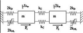

  

  Equivalent lumped-parameter model of the designed gyroscope while moving along drive direction

  Since the actuation forces are in counterphase, only one vibration mode is excited. Therefore, using the modal superposition approach, it is possible to further simplify the two-degrees-of-freedom lumped-parameter model to a one-degree-of-freedom modal system having the following mass and stiffness parameter values:

  $$ m^{*} = 2m,\,\,\,\,\,\,k^{*} = 4k_{d} + 4k_{c} + 4k_{1} ,\,\,\,\,\,\,k_{NL}^{*} = 4k_{3} ,\,\,\,\,\,\,F^{*} = F_{1} - F_{2} . $$

  This property is useful to easily synchronize sense and drive resonances, thus increasing the sensibility of the MEMS gyroscope.

• 3.26 The equation of motion is given by

  $$ \begin{aligned} & M\ddot{x} + kx\left( {1 + g\text{sgn} (x\dot{x})} \right) = 0, \\ & x(0) = a,\,\,\,\,\dot{x}(0) = 0, \\ \end{aligned} $$

  where $k$ is the spring constant and $g$ is the “nonlinearity parameter.” The “signum” function is defined as

  $$ \text{sgn} (\theta ) = \left\{ {\begin{array}{*{20}c} { + 1} & \text{for} & {\theta \;>\; 0} \\ 0 & {} & {\theta \;=\; 0} \\ { - 1} & \text{for} & {\theta \;<\; 0} \\ \end{array} } \right.. $$

• 3.27 We consider the system depicted in Fig. 3.14, composed of a chain of 10 strongly coupled linear oscillators (designated as the “primary system”) with a strongly nonlinear (nonlinearizable) end attachment [designated as the nonlinear energy sink (NES)]. The system possesses weak viscous damping, and the mass of the NES is assumed to be small, as compared with the overall mass of the chain. The governing equations of motion of the system are given by:

  $$ \begin{aligned} & \varepsilon \ddot{v} + \varepsilon \lambda (\dot{v} - \dot{y}_{0} ) + C(v - y_{0} )^{3} = 0, \\ & \ddot{y}_{0} + \varepsilon \lambda \dot{y}_{0} + \omega_{0}^{2} y_{0} - \varepsilon \lambda (\dot{v} - \dot{y}_{0} ) - C(v - y_{0} )^{3} + {\text{d}}(y_{0} - y_{1} ) = 0, \\ & \ddot{y}_{j} + \varepsilon \lambda \dot{y}_{j} + \omega_{0}^{2} y_{j} + {\text{d}}(2y_{j} - y_{j - 1} - y_{j + 1} ) = 0,\,\,\,\,\,j = 1, \ldots 8, \\ & \ddot{y}_{9} + \varepsilon \lambda \dot{y}_{9} + \omega_{0}^{2} y_{9} + {\text{d}}(y_{9} - y_{8} ) = 0, \\ \end{aligned} $$

  Fig. 3.14

  

  The chain of linear coupled oscillations (the primary system) with strongly nonlinear end attachment (the NES)

  where we introduce the small parameter $\varepsilon ,\,0\; <\; \varepsilon \;< <\; 1$ and all other parameters are assumed to be quantities of $O(1)$. In addition, we assume that the system is initially at rest and that an impulse of magnitude $F$ is applied at $t = 0$ at the left boundary of the linear chain, corresponding to the following initial conditions for the system:

  $$ \begin{aligned} & v(0) = \dot{v}(0) = 0,\,\,\,\,\,y_{p} (0) = 0,\,\,\,\,\,p = 0, \ldots ,9, \\ & \dot{y}_{k} (0) = 0,\,\,\,\,\,k = 0, \ldots ,8,\,\,\,\,\dot{y}_{9} (0 + ) = F. \\ \end{aligned} $$

• 3.28 We consider a nonlinear damping term with a fractional exponent covering the gap between viscous, dry friction, and turbulent damping phenomena.

  The equation of motion has the form

  $$ \ddot{x} \;+\; \alpha \dot{x}\left| {\dot{x}} \right|^{p - 1} \;+\; \delta x \;+\; \gamma \text{sgn} (x)\left| x \right|^{q - 1} = \mu \cos \omega t, $$

  where $x$ is displacement and $\mathop x\limits^{.}$ velocity, respectively, while the external force is

  $$ F_{x} = - \delta x - \gamma \text{sgn} (x)\left| x \right|^{q - 1} , $$

• 3.29 We consider the stochastic dynamical system

  $$ \ddot{x} + \left( {r + \alpha x^{2} - \xi (t)} \right)\dot{x} + \alpha x = - bx^{3} , $$

  where $\xi (t)$ is a white noise with intensity $D$ and the parameters $a$ and $b$ are taken to be positive in order to have a stabilizing effect.

• 3.30 The quadratically-damped Mathieu equation is

  $$ \ddot{x} + \left( {\delta + \varepsilon \cos t} \right)x + \mu \dot{x}\left| {\dot{x}} \right| = 0, $$

  where the parameter $\mu$ is assumed to be small.

  Guidance: We further expand $\delta$ and $x$ as follows:

  $$ \begin{aligned} x & = x_{0} + \mu x_{1} + \mu^{2} x_{2} + \mu^{3} x_{3} + \mu^{4} x_{4} + \mu^{5} x_{5} + \cdots \\ \delta & = \delta_{0} + \mu \delta_{1} + \mu^{2} \delta_{2} + \mu^{3} \delta_{3} + \mu^{4} \delta_{4} + \mu^{5} \delta_{5} + \cdots \\ \end{aligned} $$

  And we further introduce the parameter $\varepsilon_{1}$ defined by

  $$ \varepsilon = \varepsilon_{0} + \mu \varepsilon_{1} . $$

• 3.31 The response of a nonlinear system to harmonic excitation is governed by the equation

  $$ \ddot{x} + 2\varsigma \dot{x}\left| {\dot{x}} \right| + x + \beta \varepsilon x^{3} = \cos \frac{\Upomega }{{\omega_{0} }}t, $$

  where ${\Upomega \mathord{\left/ {\vphantom {\Upomega {\omega_{0} }}} \right. \kern-0pt} {\omega_{0} }} \approx 1$. Assume light damping $(\varsigma \ll 1)$ and weak nonlinearity $(0 < \; \varepsilon \; \ll 1)$ with

  $$ \beta = O(1). $$

• 3.32 The system considered in the present problem consists of a harmonically excited 2d system of linear coupled oscillators (with identical masses) and NES attached to it. By the term NES, we mean a small mass (relative to the linear oscillator mass) attached via essentially a nonlinear spring (pure cubic nonlinearity) and linear viscous damper to the linear subsystem, as illustrated in Fig. 3.15.

  Fig. 3.15

  

  Mechanical model of the system

  As was mentioned above, masses of linear oscillators are identical and, therefore, may be taken as unity without loss of generality $(M = 1)$. The system is described by the following equations:

  $$ \begin{aligned} & \ddot{y}_{2} + k_{2} y_{2} + k_{1} (y_{2} - y_{1} ) = \varepsilon F_{2} \cos (\omega t), \\ & \ddot{y}_{1} + k_{2} y_{1} + k_{1} (y_{1} - y_{2} ) + \varepsilon k_{v} (y_{1} - v)^{3} + \varepsilon \lambda (\dot{y}_{1} - \dot{v}) = \varepsilon F_{1} \cos (\omega t), \\ & \varepsilon \ddot{v} + \varepsilon k_{v} (v - y_{1} )^{3} + \varepsilon \lambda (\dot{v} - \dot{y}_{1} ) = 0, \\ \end{aligned} $$

  where $y_{1} ,y_{2} ,v$ are the displacements of the linear oscillators and NES, respectively, $\varepsilon \lambda$ is the damping coefficient, and $\varepsilon F_{i} (i = 1,2)$ are the amplitudes of excitation of each linear oscillator.

• 3.33 To show the response of a nonlinear oscillator under a harmonic excitation, we consider the weakly nonlinear system

  $$ \ddot{u} + \mu \dot{u} + \omega^{2} u + \mu_{3} \dot{u}\,^{3} + \alpha_{2} u^{2} + \alpha_{3} u^{3} + \alpha_{4} u^{4} + \alpha_{5} u^{5} = F\cos (\Upomega t + \gamma ), $$

  where $\dot{u} = {{{\text{d}}u} \mathord{\left/ {\vphantom {{{\text{d}}u} {{\text{d}}t}}} \right. \kern-0pt} {{\text{d}}t}}$, $t$ is the time, $\alpha_{i}$ are constants, $\mu$ and $\mu_{3}$ are damping coefficients, $F$ is the excitation amplitude, $\omega$ is the linear natural frequency, $\Upomega ( \approx \omega )$ is the excitation frequency, and $\gamma$ is the phase angle of the excitation w.r.t. the response.

• 3.34 Consider a nonlinear oscillator in the form

  $$ u^{\prime \prime } + \omega_{n}^{2} u + \mu u^{3} = F_{0} \cos (\omega t) $$

  with the initial condition

  $$ u(0) = A,\;u^{\prime} (0) = 0 $$

• 3.35 Consider the nonlinear cubic-quintic Duffing equation, which reads

  $$ u^{\prime \prime } + f(u) = 0 \, , \, f(u) = \alpha u + \beta u^{3} + \gamma u^{5} $$

  with the initial conditions

  $$ u(0) = A{ , }\;\frac{{{\text{d}}u}}{{{\text{d}}t}}(0) = 0. $$

• 3.36 We assume that the anchor spring is nonlinear with a force–displacement relation (see Fig. 3.16):

  $$ f = \delta + \delta^{3} . $$

  Fig. 3.16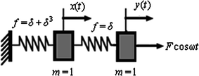

  

  Forced mass–spring system with nonlinear spring

  The second spring is assumed to be linear with characteristics $f = \delta$. The equations of motion are given by

  $$ \frac{{{\text{d}}^{2} x}}{{{\text{d}}t^{2} }} + 2x - y + x^{3} = 0,\,\,\,\,\,\frac{{{\text{d}}^{2} y}}{{{\text{d}}t^{2} }} + y - x = F\cos \omega t $$

• 3.37 Consider the nonlinear oscillator in Fig. 3.17.

  Fig. 3.17

  

  Geometry of the problem

  This oscillator is very applicable in automobile design where a horizontal motion is converted into a vertical once or vice versa.

  The equation of motion and appropriate initial conditions for this case can be given as

  $$ \begin{aligned} & (1 + Ru(t)^{2} )\,\left( {\frac{{{\text{d}}^{2} }}{{{\text{d}}t^{2} }}u(t)} \right) + Ru(t)\,\left( {\frac{\text{d}}{{{\text{d}}t}}u(t)} \right)^{2} + \omega_{0}^{2} u(t) + \frac{1}{2}\frac{{Rgu(t)^{3} }}{l} = 0 \\ & u(0) = A,\frac{{{\text{d}}u}}{{{\text{d}}t}}\,\,(0) = 0, \\ \end{aligned} $$

  where

  $$ \omega_{0}^{2} = \frac{k}{{m_{1} }} + \frac{Rg}{l},\,\,\,R = \frac{{m_{2} }}{{m_{1} }}. $$

• 3.38 We consider the motion of a ring of mass $m$ sliding freely on the wire described by the parabola $y = qu^{2}$, which rotates with a constant angular velocity $\lambda$ about the y-axis. The equation describing the motion of the ring is

  $$ \ddot{u} + \omega^{2} u = - 4qu(u\ddot{u} + \dot{u}\,^{2} ), $$

  where $\omega^{2} = 2gq - \lambda^{2}$ and the initial conditions are $u(0) = A,\,\,\,\dot{u}(0) = 0$.

• 3.39 The generalized Huxley equation

  $$ u_{t} - u_{xx} = \beta \,u(1 - u^{\delta } )(u^{\delta } - \gamma ),\,\,\,\,\,0 \le x \le 1,\,\,\,\,\,t \ge 0 $$

  with the initial condition

  $$ u(x,0) = \left[ {\frac{\gamma }{2} + \frac{\gamma }{2}\tanh (\sigma \,\gamma x)} \right]^{{\frac{1}{\delta }}} $$

  .

• 3.40 This problem considers a nonlinear oscillator with discontinuity,

  $$ \frac{{{\text{d}}^{2} x}}{{{\text{d}}t^{2} }} + \text{sgn} (x) = 0 $$

  with initial conditions

  $$ x(0) = A\,\,\,\,\,\text{and}\,\,\,\,\,\frac{{{\text{d}}x}}{{{\text{d}}t}}(0) = 0 $$

  and $\text{sgn} (x)$ defined by

  $$ \text{sgn} (x) = \left\{ \begin{gathered} - 1,\,\,\,\,\,x < 0, \hfill \\ + 1,\,\,\,\,\,x \ge 0. \hfill \\ \end{gathered} \right. $$

• 3.41 Here, a system consisting of a block of mass m that hangs from a viscous damper with coefficient c and a nonlinear spring of stiffness $k_{1}$ and $k_{3}$ is considered. The equation of motion is given by the nonlinear differential equation

  $$ \frac{{{\text{d}}^{2} x(t)}}{{{\text{d}}t^{2} }} + \frac{{k_{1} }}{m}\,x(t) + \frac{{k_{3} }}{m}\,x^{3} (t) + \frac{c}{m}\frac{{{\text{d}}x(t)}}{{{\text{d}}t}}\, = 0, $$

  with the initial conditions

  $$ x_{0} (0) = A,\,\,\,\,\,\frac{{{\text{d}}x_{0} }}{{{\text{d}}t}}(0) = 0. $$

• 3.42 In this problem, we shall consider a system consisting of a (1+1)-dimensional long-wave equation:

  $$ \begin{aligned} & u_{t} + uu_{x} + v_{x} = 0, \\ & v_{t} + (vu)_{x} + \frac{1}{3}u_{xxx} = 0 \\ \end{aligned} $$

  with the initial conditions of $u(x,0) = f(x)$ and $v(x,0) = g(x)$, where $v$ is the elevation of the water wave and $u$ is the surface velocity of water along the $x$-direction.

References

Abdel-Halim Hassan, I.H.: Different applications for differential transformation in the differential equations. J. Appl. Math. Comput. 129, 183–201 (2002)
Adomian, G.: New approach to nonlinear partial differential equations. J. Math. Anal. Appl. 102, 420–434 (1984)
Adomian, G.: A review of the decomposition method and some recent results for nonlinear equations. Math. Comput. Model. 13(7), 17–43 (1992)
Adomian, G.: Solving Frontier Problems of Physics: The Decomposition Method. Kluwer Academic Publishers, Boston (1994a)
Adomian, G.: Solution of physical problems by decomposition. Comput. Math. Appl. 27, 145–154 (1994b)
Ayaz, F.: Solutions of the system of differential equations by differential transform method. Appl. Math. Comput. 147, 547–567 (2004)
Baker, G.A. Jr.: Essentials of Padé Approximants in Theoretical Physics, pp. 27–38. Academic Press, New York (1975)
Fereidoon, A., Kordani, N., Rostamiyan, Y., Ganji, D.D.: Analytical solution to determine displacement of nonlinear oscillations with parametric excitation by differential transformation method. Math. Comput. Appl. 15(5), 810–815 (2010)
Ganji, D.D.: Approximate analytical solutions to nonlinear oscillators using He’s amplitude-frequency formulation. Int. J. Math. Anal. 4(32), 1591–1597 (2010)
Ganji, D.D., Esmaeilpour, M.: Soheil Soleimani: approximate solutions to Van der Pol damped nonlinear oscillators by means of He’s energy balance method. Int. J. Comput. Math. 87(9), 2014–2023 (2010)
Ganji, D.D., Kachapi, S.H.H.: Analysis of Nonlinear Equations in Fluids, Progress in Nonlinear Science, vol. 3, pp. 1–293. Asian Academic Publisher Limited, Hong Kong (2011a)
Ganji, D.D., Kachapi, S.H.H.: Analytical and Numerical Methods in Engineering and Applied Sciences, Progress in Nonlinear Science, vol. 3, pp. 1–579. Asian Academic Publisher Limited, Hong Kong (2011b)
Ganji, D.D., Kachapi, S.H.H.: Nonlinear Analysis in Science and Engineering. Cambridge International Science Publisher, Cambridge (in press, 2013a)
Ganji, D.D., Kachapi, S.H.H.: Nonlinear Differential Equations: Analytical Methods and Application. Cambridge International Science Publisher associated with Springer (in press, 2013b)
Ganji, D.D., Nourollahi, M., Rostamian, M.: A comparison of variational iteration method with Adomian’s decomposition method in some highly nonlinear equations. Int. J. Sci. Technol. 2(2), 179–188 (2007)
Ganji, S.S., Sfahani, M.G., Modares Tonekaboni, S.M., Moosavi, A.K., Ganji, D.D.: Higher-order solutions of coupled systems using the parameter expansion method. Math. Probl. Eng. 2009, Article ID 327462, 1–20 (2009a)
Ganji, S.S., Ganji, D.D., Ganji, Z.Z., Karimpour, S.: Periodic solution for strongly nonlinear vibration systems by He’s energy balance method. Acta Applicandae Mathematicae 106(1), 79–92 (2009b). doi:10.1007/s10440-008-9283-6
Ganji, S.S., Ganji, D.D., Babazadeh, H., Sadoughi, N.: Application of amplitude- frequency formulation to nonlinear oscillation system of the motion of a rigid rod rocking back. Math. Methods Appl. Sci. 33(2), 157–166 (2010a)
Ganji, D.D., Alipour, M.M., Fereidoon, A.H., Rostamiyan, Y.: Analytic approach to investigation of fluctuation and frequency of the oscillators with odd and even nonlinearities. IJE Trans. A: Basics 23, 41–56 (2010b)
Gupta, V.H., Munjal, M.L.: On numerical prediction of the acoustic source characteristics of an engine exhaust system. J. Acoust. Soc. Am. 92(5), 2716–2725 (1992)
Hassan, I.H.A.H.: On solving some eigenvalue-problems by using a differential transformation. Appl. Math. Comput. 127(1), 1–22 (2002)
Hassan, I.H.A.H.: Differential transformation technique for solving higher-order initial value problems. Appl. Math. Comput. 154(2), 299–311 (2004)
He, J.H.: Bookkeeping parameter in perturbation methods. Int. J. Non-linear Sci. Numer. Simul. 2, 257–264 (2001a)
He, J.H.: Modified Lindstedt–Poincare methods for some non-linear oscillations. Part III: double series expansion. Int. J. Non-linear Sci. Numer. Simul. 2, 317–320 (2001b)
He, J.H.: Modified Lindstedt–Poincare methods for some strongly non-linear oscillations. Part II: a new transformation. Int. J. Non-linear Mech. 37(2), 309–314 (2002)
He, J.-H.: Solution of nonlinear equations by an ancient Chinese algorithm. Appl. Math. Comput. 151(1), 293–297 (2004)
Kimiaeifar, A., Saidi, A.R., Bagheri, G.H., Rahimpour, M., Domairry, D.G.: Analytical solution for Van der Pol–Duffing oscillators. Chaos, Solitons & Fractals 42(5), 2660–2666 (2009a)
Kimiaeifar, A., Saidi, A.R., Sohouli, A.R., Ganji, D.D.: Analysis of modified Van der Pol’s oscillator using He’s parameter-expanding methods. Curr. Appl. Phys 10 (2010)
Liu, L., Dowell, E.H.: Harmonic balance approach for an airfoil with a freeplay control surface. AIAA J. 43(4), 802 (2005)
Liu, H., Song, Y.: Differential transform method applied to high index differential-algebraic equations. Appl. Math. Comput. 184, 748–753 (2007)
Liu, L., Thomas, J.P., Dowell, E.H., Attar, P., Hall, K.C.: A comparison of classical and high dimensional harmonic balance approaches for a Duffing oscillator. J. Comput. Phys. 215(1), 298–320 (2006)
Luo, X.-G.: A two-step Adomian decomposition method. Appl. Math. Comput. 170(1), 570–583 (2005)
Momani, S., Ertürk, V.S.: Solutions of non-linear oscillators by the modified differential transform method. Comput. Math. Appl. 55(4), 833–842 (2008)
Momeni, M., Jamshidi, N., Barari, A., Ganji, D.D.: Application of He’s energy balance method to Duffing-harmonic oscillators. Int. J. Comput. Math. 88(1), 135–144 (2011a)
Momeni, M., Jamshidi, N., Barari, A., Ganji, D.D.: Application of He’s energy balance method to Duffing-harmonic oscillators. Int. J. Comput. Math. 88(1), 135–144 (2011b)
Nayfeh, A.H.: Perturbation Methods. Wiley, New York (2000)
Ragulskis, M., Fedaravicius, A., Ragulskis, K.: Harmonic balance method for FEM analysis of fluid flow in a vibrating pipe. Commun. Numer. Methods Eng. 22(5), 347–356 (2006)
Sadighi, A., Ganji, D.D.: Exact solutions of Laplace equation by homotopy-perturbation and Adomian decomposition methods. Phys. Lett. A 367(1–2), 83–87 (2007)
Sadighi, A., Ganji, D.D.: Analytic treatment of linear and nonlinear Schrödinger equations: a study with homotopy-perturbation and Adomian decomposition methods. Phys. Lett. A 372(4), 465–469 (2008a)
Sadighi, A., Ganji, D.D.: A study on one dimensional nonlinear thermoelasticity by Adomian decomposition method. World J. Model. Simul. 4(1), 19–25 (2008b)
Sadighi, A., Ganji, D.D., Sabzehmeidani, Y.: A decomposition method for volume flux and average velocity of thin film flow of a third grade fluid down an inclined plane. Adv. Theor. Appl. Mech. 1(1), 45–59 (2008)
Safari, M., Ganji, D.D., Moslemi, M.: Application of He’s variational iteration method and Adomian’s decomposition method to the fractional KdV-Burgers-Kuramoto equation. Comput. Math. Appl. 58(11–12), 2091–2097 (2009)
Telli, S., Kopmaz, O.: Free vibrations of a mass grounded by linear and non-linear springs in series. J. Sound Vib. 289, 689–710 (2006)
Wang, S.-Q., He, J.-H.: Nonlinear oscillator with discontinuity by parameter-expansion method. Chaos, Solitons Fractals 35, 688–691 (2008)
Wazwaz, A.M.: The modified decomposition method and the Pade approximants for solving Thomas–Fermi equation. Appl. Math. Comput. 105, 11–19 (1999a)
Wazwaz, A.M.: A reliable modification of Adomian decomposition method. Appl. Math. Comput. 102, 77–86 (1999b)
Wazwaz, A.M.: Construction of solitary wave solutions and rational solutions for the KdV equation by Adomian decomposition method. Chaos, Solitons Fractals 12, 2283–2293 (2001)
Wu, D.M., Wang, Z.: A Mathematica program for the approximate analytical solution to a nonlinear undamped Duffing equation by a new approximate approach. Comput. Phys. Commun. 174(6), 447–463 (2006)
Zhang, B.-Q., Luo, X.-G., Wu, Q.-B.: The restrictions and improvement of the Adomian decomposition method. Appl. Math. Comput. 171(1), 99–104 (2006)
Zhou, J.K.: Differential Transformation and its Applications for Electrical Circuits. Huazhong University Press, Wuhan (1986). (in Chinese)
Author information
Authors and Affiliations
Corresponding author
Rights and permissions
Copyright information
© 2014 Springer Science+Business Media B.V.
About this chapter
Cite this chapter
Hashemi, S.H., Domairry, D. (2014). Considerable Analytical Methods. In: Dynamics and Vibrations. Solid Mechanics and Its Applications, vol 202. Springer, Dordrecht. https://doi.org/10.1007/978-94-007-6775-1_3
Download citation
DOI: https://doi.org/10.1007/978-94-007-6775-1_3
Published:
Publisher Name: Springer, Dordrecht
Print ISBN: 978-94-007-6774-4
Online ISBN: 978-94-007-6775-1
eBook Packages: EngineeringEngineering (R0)