Computation of the Szeged Index of Some Nanotubes and Dendrimers

Abstract

Let e be an edge of a G connecting the vertices u and v. Define two sets ${N_1}\left( {\left. e \right|G} \right)$ and ${N_2}\left( {\left. e \right|G} \right)$ as ${N_1}\left( {\left. e \right|G} \right)=\left\{ {\left. {x\in V(G)} \right|\mathrm{d}\left( {x,u} \right)<\mathrm{d}\left( {x,v} \right)} \right\}$ and ${N_2}\left( {\left. e \right|G} \right)=\left\{ {\left. {x\in V(G)} \right|\mathrm{d}\left( {x,v} \right)<\mathrm{d}\left( {x,u} \right)} \right\}$. The number of elements of ${N_1}\left( {\left. e \right|G} \right)$ and ${N_2}\left( {\left. e \right|G} \right)$ are denoted by ${n_1}\left( {\left. e \right|G} \right)$ and ${n_2}\left( {\left. e \right|G} \right)$, respectively. The Szeged index of the graph G is defined as $\mathrm{Sz}(G)=\sum\nolimits_{{e\in E(G)}} {{n_1}\left( {\left. e \right|G} \right){n_2}\left( {\left. e \right|G} \right)}$.

In this chapter, we compute the Szeged index of some types of dendrimers, for example, dendrimer nanostars, Styrylbenzene dendrimer, Triarylamine Dendrimer of Generation 1–3, and then we compute the Szeged index of some nanotubes, for example, TUC₄C₈(R) and TUC₄C₈(S) nanotubes, Armchair Polyhex nanotube, and HAC₅C₆C₇[k; p], V C₅C₇[p; q], and HC₅C₇[p; q] nanotubes.

These keywords were added by machine and not by the authors. This process is experimental and the keywords may be updated as the learning algorithm improves.

12.1 Introduction

Dendrimers are large and complex molecules with very well-defined chemical structures. From a polymer chemistry point of view, dendrimers are nearly perfect monodisperse (basically meaning of a consistent size and form) macromolecules with a regular and highly branched three-dimensional architecture. They consist of three major architectural components: core, branches, and end groups. Dendrimers are produced in an iterative sequence of reaction steps (Holister and Harper 2003). In 1985, the interest in this research field started to grow exponentially:

More than 1,000 articles have been published in 2002 concerning the various aspects of dendrimer chemistry. We can consider the figure of dendrimers as the shape of a molecular graph.

A graph $G$ consists of a set of vertices $V(G)$ and a set of edges $E(G)$. In chemical graphs, each vertex represented an atom of the molecule, and covalent bonds between atoms are represented by edges between the corresponding vertices. This shape derived from a chemical compound is often called its molecular graph, and can be a path, a tree, or in general a graph.

A topological index is a single number, derived following a certain rule, which can be used to characterize the molecule. Usage of topological indices in biology and chemistry began in 1947 when chemist Harold Wiener (1947) introduced Wiener index to demonstrate correlations between physicochemical properties of organic compounds and the index of their molecular graphs. Wiener originally defined his index ($W$) on trees and studied its use for correlation of physicochemical properties of alkenes, alcohols, amines, and their analogous compounds. A number of successful QSAR studies have been made based in the Wiener index and its decomposition forms (Agrawal et al. 2000).

Another topological index was introduced by Gutman and called the Szeged index, abbreviated as Sz (Gutman 1994).

Let $e$ be an edge of a graph $G$ connecting the vertices $u$ and $v$. Define two sets ${N_1}\left( {e\left| G \right.} \right)$ and ${N_2}\left( {e\left| G \right.} \right)$ as ${N_1}\left( {e\left| G \right.} \right)=\{\left. {x\in V(G)} \right|\mathrm{d}(u,x)<\mathrm{d}(v,x)\}$ and ${N_2}\left( {e\left| G \right.} \right)=\{\left. {x\in V(G)} \right|\mathrm{d}(x,v)<\mathrm{d}(x,u)\}$. The number of elements of ${N_1}(e\left| G \right.)$ and ${N_2}(e\left| G \right.)$ are denoted by ${n_1}(e\left| G \right.)$ and ${n_2}(e\left| G \right.)$, respectively. The Szeged index of the graph $G$ is defined as $\mathrm{Sz}(G)=\mathrm{Sz}=\sum\nolimits_{{e\in E(G)}} {{n_1}\left( {e\left| G \right.} \right){n_2}\left( {e\left| G \right.} \right)}$. The Szeged index is a modification of Wiener index to cyclic molecules. The Szeged index was conceived by Gutman at the Attila Jozsef University in Szeged. This index received considerable attention. It has attractive mathematical characteristics (Diudea et al. 2004).

In this chapter, in Sect. 12.2, we compute the Szeged index of some types of dendrimers, for example, Naphthalene dendrimer, Styrylbenzene dendrimer, dendrimer nanostars, and then in Sect. 12.3, we compute the Szeged index of some nanotubes, for example, TUC₄C₈(R) and TUC₄C₈(S) nanotubes, Armchair Polyhex nanotube, and HAC₅C₆C₇[k; p], VC₅C₇[p; q], and HC₅C₇[p; q] nanotubes.

12.2 Computation of Szeged Index of Some Type of Dendrimers

In this section, at first we compute the Szeged index of the first, second, third, and fourth type of dendrimer nanostars. All of the results in the first part of this section have been published in Iranmanesh and Gholami (2007, 2008).

In the second part, we compute the Szeged index of the Styrylbenzene dendrimers, Triarylamine Dendrimer of Generation 1–3, and a Naphthalene dendrimer. All of the results in the second part of this section have been published in Iranmanesh and Gholami (2009) and Iranmanesh et al. (2010).

12.2.1 Computing the Szeged Index of First-Type Nanostar

Figure 12.1 shows a first-type nanostar which has grown n stages.

Fig. 12.1

First-type nanostar

In Fig. 12.1, we show the graph of this nanostar. In this figure we have 1 nucleus and a central hexagon denoted by $h_0^0$. In stages 1 and 2, we denoted the hexagons and edges by $h_i^j$, where $1\leq i\leq 2,\,\,1\leq j\leq 3$, and in the other stages, we denoted the hexagons and edges by ${h_j}$ and ${e_j}$. The growth of this nanostar from stage 3 is the same, and we have only two hexagons in each stage. Now, we start the computing of the Szeged index of this nanostar from stage n. Suppose that e is an edge of the hexagon ${h_n}$; for all of the edges of ${h_n}$, we have ${n_1}\left( {e|G} \right)=3$; also the number of these hexagons is ${2^n}$. Suppose further that e is an edge of ${h_{n-1 }}$; for 4 of these edges we have ${n_1}\left( {e|G} \right)=1\times 6+3$, and for the other 2 edges we have ${n_1}\left( {e|G} \right)=2\times 6+3$; also the number of these hexagons is ${2^{n-1 }}$. Now assume that e is an edge of ${h_k}$ so that $3\leq k\leq n$; in this case, for 4 of the edges we have ${n_1}\left( {e|G} \right)=\left( {{2^{n-k }}-1} \right)\times 6+3$, and for the other 2 edges we have ${n_1}\left( {e|G} \right)=2\times \left( {{2^{n-k }}-1} \right)\times 6+3$; the number of these hexagons is ${2^k}$. If e is an edge of $h_2^2$, for 4 of the edges we have ${n_1}\left( {e|G} \right)=\left( {{2^{n-2 }}-1} \right)\times 6+3$, and for the other 2 edges we have ${n_1}\left( {e|G} \right)=2\times \left( {{2^{n-2 }}-1} \right)\times 6+3$; the number of these hexagons is ${2^2}$. If e is an edge of $h_2^1$, for all 6 edges, ${n_1}\left( {e|G} \right)=\left( {{2^{n-1 }}-1} \right)\times 6+3$; the number of these hexagons is ${2^2}$. If e is an edge of $h_1^3$, for 4 of the edges we have ${n_1}\left( {e|G} \right)={2^{n-1 }}\times 6+3$, and for the other 2 edges we have ${n_1}\left( {e|G} \right)={2^n}\times 6+3$; the number of these hexagons is 2. If e is an edge of $h_1^2$, for all 6 edges, ${n_1}\left( {e|G} \right)=\left( {{2^n}+1} \right)\times 6+3$; the number of these hexagons is 2. If e is an edge of $h_1^1$, for all 6 edges, ${n_1}\left( {e|G} \right)=\left( {{2^n}+2} \right)\times 6+3$; the number of these hexagons is 2. If e is an edge of $h_0^0$, for 4 of the edges we have ${n_1}\left( {e|G} \right)=\left( {{2^n}+3} \right)\times 6+3$, and for the other 2 edges we have ${n_1}\left( {e|G} \right)=2\times \left( {{2^n}+3} \right)\times 6+3$. Now assuming that e is the edge ${e_n}$, we have ${n_1}\left( {{e_n}|G} \right)=6$, and the number of these edges is ${2^n}$. For the edge ${e_{n-1 }}$, we have ${n_1}\left( {{e_{n-1 }}|G} \right)=\left( {2+1} \right)\times 6$, and the number of these edges is ${2^{n-1 }}$. For the edge ${e_k}$, in a way that $3\leq k\leq n$, we have ${n_1}\left( {{e_k}|G} \right)=\left( {{2^{n-k+1 }}-1} \right)\times 6$; the number of these edges is ${2^k}$. For the edge $e_2^2$, we have ${n_1}\left( {e_2^2|G} \right)=\left( {{2^{n-1 }}-1} \right)\times 6$. For the edge $e_2^1$, we have ${n_1}\left( {e_2^1|G} \right)={2^{n-1 }}\times 6$; the number of these edges is ${2^2}$. For the edge $e_1^3$, we have ${n_1}\left( {e_1^3|G} \right)=\left( {{2^n}+1} \right)\times 6$. For the edge $e_1^2$, we have ${n_1}\left( {e_1^2|G} \right)=\left( {{2^n}+2} \right)\times 6$. For the edge $e_1^1$, we have ${n_1}\left( {e_1^1|G} \right)=\left( {{2^n}+3} \right)\times 6$; the number of these edges in stage one is 2. For the edge between the nucleus and central hexagon ($h_0^0$), we have ${n_1}\left( {e|G} \right)=\left( {{2^{n+1 }}+7} \right)\times 6$.

Now we obtain ${n_1}\left( {e|G} \right)$ for the edges of the nucleus.

According to Fig. 12.2, we have ${n_1}\left( {{e_i}|G} \right)=10$ for $i=1,2,3,4,5,6,7,8,9,10$; for $i=11,12,13,14,15,16$, we have ${n_1}\left( {{e_i}|G} \right)=3$, for $i=17,18,19,{n_1}\left( {{e_i}|G} \right)=5$, for $i=20,21,22,{n_1}\left( {{e_i}|G} \right)=15$, and for $i=23,24,{n_1}\left( {{e_i}|G} \right)=17$.

Fig. 12.2

Nucleus

The number of the vertices of this nanostar is equal to $r=\left( {{2^{n+1 }}+7} \right)\times 6+20$. But we know that ${n_2}\left( {e|G} \right)=r-{n_1}\left( {e|G} \right)$ for any of edge e. Now the Szeged index of the above nanostar is obtained in the following way:

$$ \begin{array}{llll} \mathrm{Sz}\left( {{G_n}} \right)= & \sum\limits_{k=3}^n {\left[ {{2^k}\left( \begin{gathered} 4\times \left( {\left( {{2^{n-k }}-1} \right)\times 6+3} \right)\left( {r-\left( {{2^{n-k }}-1} \right)\times 6-3} \right) \hfill \\ +2\times \left( {2\left( {{2^{n-k }}-1} \right)\times 6+3} \right)\left( {r-2\left( {{2^{n-k }}-1} \right)\times 6-3} \right) \hfill \\ \end{gathered} \right)} \right]} \\ & +{2^2}\left[ \begin{gathered} 4\times \left( {\left( {{2^{n-2 }}-1} \right)\times 6+3} \right)\left( {r-\left( {{2^{n-2 }}-1} \right)\times 6-3} \right) \hfill \\ +2\left( {2\left( {{2^{n-2 }}-1} \right)\times 6+3} \right)\left( {r-2\left( {{2^{n-2 }}-1} \right)\times 6-3} \right) \hfill \\ \end{gathered} \right] \\ & {2^2}\left[ {6\left( {\left( {{2^{n-1 }}-1} \right)\times 6+3} \right)\left( {r-\left( {{2^{n-1 }}-1} \right)\times 6-3} \right)} \right] \\ & +2\left[ \begin{gathered} 4\left( {{2^{n-1 }}\times 6+3} \right)\left( {r-{2^{n-1 }}\times 6-3} \right) \hfill \\ +2\left( {{2^n}\times 6+3} \right)\left( {r-{2^n}\times 6-3} \right) \hfill \\ \end{gathered} \right]+2\left[ {6\left( {\left( {{2^n}+1} \right)\times 6+3} \right)\left( {r-\left( {{2^n}+1} \right)\times 6-3} \right)} \right] \\ & +2\left[ {6\left( {\left( {{2^n}+2} \right)\times 6+3} \right)\left( {r-\left( {{2^n}+2} \right)\times 6-3} \right)} \right]+4\left( {\left( {{2^n}+3} \right)\times 6+3} \right)\left( {r-\left( {{2^n}+3} \right)\times 6-3} \right) \\ & +2\left( {\left( {2\left( {{2^n}+3} \right)\times 6+3} \right)} \right)\left( {r-2\left( {{2^n}+3} \right)\times 6-3} \right) \\ & +\sum\limits_{k=3}^n {\left[ {{2^k}\left( {\left( {{2^{n-k+1 }}-1} \right)\times 6\left( {r-\left( {{2^{n-k+1 }}-1} \right)\times 6} \right)} \right)} \right]} \\ & +{2^2}\left[ {\left( {{2^{n-1 }}-1} \right)\times 6\left( {r-\left( {{2^{n-1 }}-1} \right)\times 6} \right)} \right]+{2^2}\left[ {{2^{n-1 }}\times 6\left( {r-{2^{n-1 }}\times 6} \right)} \right] \\ & +2\left[ {\left( {{2^n}+1} \right)\times 6\left( {r-\left( {{2^n}+1} \right)\times 6} \right)} \right]+2\left[ {\left( {{2^n}+2} \right)\times 6\left( {r-\left( {{2^n}+2} \right)\times 6} \right)} \right] \\ & +2\left[ {\left( {{2^n}+3} \right)\times 6\left( {r-\left( {{2^n}+3} \right)\times 6} \right)} \right]+\left( {{2^{n+1 }}+7} \right)\times 6\left( {r-\left( {{2^{n+1 }}+7} \right)\times 6} \right) \\ & 10\times 10\times \left( {r-10} \right)+6\times 3\times \left( {r-3} \right)+3\times 5\times \left( {r-5} \right)+3\times 15\times \left( {r-15} \right)+2\times 17\times \left( {r-17} \right) \\ = & 41788+16812\times {2^n}+4440\times {2^n}\times n+468\times {4^n}+720\times n\times {4^n} \\ \end{array} $$

12.2.2 Computing the Szeged Index of Second-Type Nanostar

The following figure shows a second-type nanostar which has grown n stages (Fig. 12.3).

Fig. 12.3

Second-type nanostar

Let $h_i^i$ be the hexagon between hexagons ${h_i}$ and ${h_{i-1 }}$. Let $e_i^j$ be the jth edge between two hexagons in the stage i, $1\leq i\leq n,\,\,1\leq j\leq 2$. In the first step we compute ${n_1}\left( {e|G} \right)$ for ${h_i}$’s. For ${h_n}$, we have ${n_1}\left( {e|G} \right)=3$, which is the same for all of its six edges; the number of these hexagons is ${2^n}$. If e is an edge of ${h_{n-1 }}$, for 2 of the edges of the hexagon, we have ${n_1}\left( {e|G} \right)=2\times 2\times 6+3$, and for the other 4 edges, we have ${n_1}\left( {e|G} \right)=2\times 6+3$; the number of these hexagons is ${2^{n-1 }}$. Now assume that e is an edge of ${h_{k-1 }},\,1\leq k\leq n$; for 2 of the edges we have ${n_1}\left( {e|G} \right)=2\times \left( {{2^{{n-\left( {k-1} \right)}}}+{2^{n-k }}+\cdots +2} \right)\times 6+3=2\times \left( {{2^{n-k+2 }}-2} \right)\times 6+3$ and for the other 4, ${n_1}\left( {e|G} \right)=\left( {{2^{{n-\left( {k-1} \right)}}}+{2^{n-k }}+\cdots +2} \right)\times 6+3=\left( {{2^{n-k+2 }}-2} \right)\times 6+3$; the number of these hexagons is ${2^{{\left( {k-1} \right)}}}$. Now we compute ${n_1}\left( {e|G} \right)$ for $h_i^i$’s. For all of six edges of $h_n^n$, we have ${n_1}\left( {e|G} \right)=9$; the number of these hexagons is ${2^n}$. If e is an edge of $h_{n-1}^{n-1 }$, for all six edges, ${n_1}\left( {e|G} \right)=\left( {{2^2}+1} \right)\times 6+3$, the number of this hexagon is ${2^{n-1 }}$. If e is an edge of $h_k^k$, $1\leq k\leq n-1$, for all of the six edges, ${n_1}\left( {e|G} \right)=\left( {{2^{n-k+1 }}+{2^{n-k }}+\cdots +{2^2}+1} \right)\times 6+3=\left( {{2^{n-k+2 }}-3} \right)\times 6+3$, the number of these hexagons is ${2^k}$. Now ${n_1}\left( {e|G} \right)$ is computed for $e_i^j$. For the edge $e_n^2$, ${n_1}\left( {e_n^2|G} \right)=1\times 6$. For the edge $e_n^1$, ${n_1}\left( {e_n^1|G} \right)=2\times 6$; the number of these edges is ${2^n}$. For the edge $e_{n-1}^2$, ${n_1}\left( {e_{n-1}^2|G} \right)=\left( {{2^2}+1} \right)\times 6$. For the edge $e_{n-1}^1$, ${n_1}\left( {e_{n-1}^1|G} \right)=\left( {{2^2}+2} \right)\times 6$; the number of these edges is ${2^{n-1 }}$. For the edge $e_k^2$, we have ${n_1}\left( {e_k^2|G} \right)=\left( {{2^{n-k+2 }}-3} \right)\times 6$, and ${n_1}\left( {e|G} \right)$ for the edges $e_i^1$ is as follows: for the edge $e_k^1$, we have ${n_1}\left( {e_k^1|G} \right)=\left( {{2^{n-k+2 }}-2} \right)\times 6$; the number of these edges is ${2^k}$. Therefore, we have computed ${n_1}\left( {e|G} \right)$ for all of the edges of this nanostar. The number of the vertices of this nanostar is equal to $r=\left( {{2^{n+2 }}-3} \right)\times 6$. But we know that ${n_2}\left( {e|G} \right)=r-{n_1}\left( {e|G} \right)$ for any of edge e. Now its Szeged index is obtained easily.

$$ \begin{array}{llll} \mathrm{Sz}\left( {{G_n}} \right)= & \sum\limits_{k=1}^n {\left[ {{2^{k-1 }}\times \left( \begin{gathered} 2\times \left( {2\times \left( {{2^{n-k+2 }}-2} \right)\times 6+3} \right)\left( {r-2\times \left( {{2^{n-k+2 }}-2} \right)\times 6-3} \right) \hfill \\ +4\times \left( {\left( {{2^{n-k+2 }}-2} \right)\times 6+3} \right)\left( {r-\left( {{2^{n-k+2 }}-2} \right)\times 6-3} \right) \hfill \\ \end{gathered} \right)} \right]} \\ & +\sum\limits_{k=1}^{n-1 } {\left[ {{2^k}\left( {6\times \left( {\left( {{2^{n-k+2 }}-3} \right)\times 6+3} \right)} \right)\left( {r-\left( {{2^{n-k+2 }}-3} \right)\times 6-3} \right)} \right]} \\ & +{2^n}\left( {6\times \left( {9\left( {r-9} \right)+3\left( {r-3} \right)} \right)} \right) \\ & +\sum\limits_{k=1}^n {\left[ {{2^k}\left( {\left( {{2^{n-k+2 }}-3} \right)\times 6} \right)\left( {r-\left( {{2^{n-k+2 }}-3} \right)\times 6} \right)} \right]} \\ & +\sum\limits_{k=1}^n {\left[ {{2^k}\left( {\left( {{2^{n-k+2 }}-2} \right)\times 6} \right)\left( {r-\left( {{2^{n-k+2 }}-2} \right)\times 6} \right)} \right]} \\ = & -882+6912\times {4^n}\times n-15264\times {4^n}+3456\times {2^n}\times n+16200\times {2^n} \\ \end{array} $$

12.2.3 Computing the Szeged Index of Three-Type Nanostar

Figure 12.4 shows a three-type nanostar which has grown n stages.

Fig. 12.4

Three-type nanostar

In Fig. 12.4, we show that the shape of this nanostar. In this figure we have 1 nucleus and a central hexagon denoted by ${h_0}$. We denoted the hexagons and edges by ${h_i}$ and ${e_i}$. Now, we start the computing of the Szeged index of this nanostar from stage n. Suppose that e is an edge of the hexagon ${h_n}$; for all of edges of ${h_n}$, we have ${n_1}\left( {e|G} \right)=3$; also the number of these hexagons is ${2^n}$. Suppose further that e is an edge of ${h_{n-1 }}$; for 4 of these edges we have ${n_1}\left( {e|G} \right)=1\times 6+3=9$, and for the other 2 edges we have ${n_1}\left( {e|G} \right)=2\times 6+3=15$; also the number of these hexagons is ${2^{n-1 }}$. Suppose that e is an edge of ${h_k}$; for 4 of the edges we have ${n_1}\left( {e|G} \right)=\left( {{2^{n-k }}-1} \right)\times 6+3$, and for the other 2 edges we have ${n_1}\left( {e|G} \right)=2\times \left( {{2^{n-k }}-1} \right)\times 6+3$; the number of these hexagons is ${2^k}$.

Now ${n_1}\left( {e|G} \right)$ is computed for ${e_i}$. Suppose e is the edge ${e_n}$, we have ${n_1}\left( {{e_n}|G} \right)=1\times 6=6$; the number of these edges is ${2^n}$. For the edge ${e_{n-1 }}$, we have ${n_1}\left( {{e_{n-1 }}|G} \right)=\left( {2+1} \right)\times 6=18$; the number of these edges is ${2^{n-1 }}$. For the edge ${e_k},\,\,1\leq k\leq n$, we have ${n_1}\left( {{e_k}|G} \right)=\left( {{2^{n-k+1 }}-1} \right)\times 6$; the number of these edges is ${2^k}$. For the edge between the nucleus and central hexagon (${h_0}$), we have ${n_1}\left( {e|G} \right)=\left( {{2^{n+1 }}-1} \right)\times 6$.

Now we obtain ${n_1}\left( {e|G} \right)$ for the edges of the nucleus.

According to Fig. 12.2, we have computed ${n_1}\left( {e|G} \right)$ for all of the edges of this nanostar. The number of the vertices of this nanostar is equal to $r=\left( {{2^{n+1 }}-1} \right)\times 6+20$. But we know that ${n_2}\left( {e|G} \right)=r-{n_1}\left( {e|G} \right)$ for any edge e. Now the Szeged index of the above nanostar is obtained in the following way:

$$ \begin{array}{llll} \mathrm{Sz}\left( {{G_n}} \right)= & \sum\limits_{k=0}^n {\left[ {{2^k}\left( \begin{gathered} 2\times \left( {\left( {2\times \left( {{2^{n-k }}-1} \right)\times 6+3} \right)\left( {r-2\times \left( {{2^{n-k }}-1} \right)\times 6-3} \right)} \right) \hfill \\ +4\times \left( {\left( {{2^{n-k }}-1} \right)\times 6+3} \right)\left( {r-\left( {{2^{n-k }}-1} \right)\times 6-3} \right) \hfill \\ \end{gathered} \right)} \right]} \\ & +\sum\limits_{k=0}^n {\left[ {{2^k}\left( {\left( {\left( {{2^{n-k+1 }}-1} \right)\times 6} \right)\left( {r-\left( {{2^{n-k+1 }}-1} \right)\times 6} \right)} \right)} \right]} \\ & +10\times 10\times \left( {r-10} \right)+6\times 3\times \left( {r-3} \right)+3\times 5\times \left( {r-5} \right)+3\times 15\times \left( {r-15} \right)+2\times 17\times \left( {r-17} \right) \\ = & 3636\times {2^n}+1324+720\times n\times {4^n}+1560\times n\times {2^n}-1296\times {4^n} \\ \end{array} $$

12.2.4 Computing the Szeged Index of Four-Type Nanostar

Figure 12.5 shows a four-type nanostar which has grown four stages.

Fig. 12.5

Four-type nanostar

In this figure, we have 1 nucleus and a central hexagon denoted by ${h_0}$. Let $h_i^j$ be the ith hexagon in stage j, $1\leq j\leq n,\,\,1\leq i\leq 3$, and let $e_i^j$ be the ith edge between two hexagons in stage j. Now, we start the computing of the Szeged index of this nanostar from stage n. Suppose that e is an edge of the hexagon $h_3^n$; for all of edges of $h_3^n$, we have ${n_1}\left( {e|G} \right)=3$; for all of edges of $h_2^n$, we have ${n_1}\left( {e|G} \right)=6+3=9$; for all of edges of $h_1^n$, we have ${n_1}\left( {e|G} \right)=2\times 6+3=15$; also the number of these hexagons is ${2^n}$. Suppose that e is an edge of the hexagon $h_3^{n-1 }$; for 4 of these edges we have ${n_1}\left( {e|G} \right)=3\times 6+3=21$, and for the other 2 edges we have ${n_1}\left( {e|G} \right)=2\times 3\times 6+3=39$; for all of edges of $h_2^{n-1 }$, we have ${n_1}\left( {e|G} \right)=2\times 3\times 6+6+3=45$; for all of edges of $h_1^{n-1 }$, we have ${n_1}\left( {e|G} \right)=2\times 3\times 6+2\times 6+3=51$; also the number of these hexagons is ${2^{n-1 }}$. We continue until to achieve stage 1. Suppose that e is an edge of the hexagon $h_3^1$; for 4 of these edges we have

$$ \begin{array}{llll} {n_1}\left( {e|G} \right)= & 3\times \left( {{2^{n-2 }}+{2^{n-3 }}+\cdots +2+1} \right)\times 6+3 \\ = & 3\times \left( {{2^{n-1 }}-1} \right)\times 6+3, \\ \end{array} $$

and for other 2 edges, we have

$$ \begin{array}{llll} {n_1}\left( {e|G} \right)= & 3\times \left( {{2^{n-1 }}+{2^{n-2 }}+\cdots +2} \right)\times 6+3 \\ = & 3\times \left( {{2^n}-2} \right)\times 6+3; \\ \end{array} $$

for all of edges of $h_2^1$, we have

$$ \begin{array}{llll} {n_1}\left( {e|G} \right)= & 3\times \left( {{2^{n-1 }}+{2^{n-2 }}+\cdots +2} \right)\times 6+6+3 \\ = & 3\times \left( {{2^n}-2} \right)\times 6+9; \\ \end{array} $$

for all of edges of $h_1^1$, we have

$$ \begin{array}{llll} {n_1}\left( {e|G} \right)= & 3\times \left( {{2^{n-1 }}+{2^{n-2 }}+\cdots +2} \right)\times 6+2\times 6+3 \\ = & 3\times \left( {{2^n}-2} \right)\times 6+15; \\ \end{array} $$

also the number of these hexagons is 2. Suppose that e is an edge of the hexagon ${h_0}$; for 4 of these edges we have

$$ \begin{array}{llll} {n_1}\left( {e|G} \right)= & 3\times \left( {{2^{n-1 }}+\cdots +2+1} \right)\times 6+3 \\ = & 3\times \left( {{2^n}-1} \right)\times 6+3, \\ \end{array} $$

and for the other 2 edges we have

$$ \begin{array}{llll} {n_1}\left( {e|G} \right)= & 3\times \left( {{2^n}+{2^{n-1 }}+\cdots +2} \right)\times 6+3 \\ = & 3\times \left( {{2^{n+1 }}-2} \right)\times 6+3. \\ \end{array} $$

Now ${n_1}\left( {e|G} \right)$ is computed for $e_j^i$. Suppose e is the edge $e_3^n$, we have ${n_1}\left( {e_3^n|G} \right)=6={a_1}$; for the edge $e_2^n$, we have ${n_1}\left( {e_2^n|G} \right)={a_1}+6$; for the edge $e_1^n$, we have ${n_1}\left( {e_1^n|G} \right)={a_1}+12$; the number of these edges is ${2^n}$. Suppose e is the edge $e_3^{n-1 }$, we have ${n_1}\left( {e_3^{n-1 }|G} \right)=3\times 2\times 6+6=42={a_2}$; for the edge $e_2^{n-1 }$, we have ${n_1}\left( {e_2^{n-1 }|G} \right)={a_2}+6$; for the edge $e_1^{n-1 }$, we have ${n_1}\left( {e_1^{n-1 }|G} \right)={a_2}+12$; the number of these edges is ${2^{n-1 }}$. We continue until to achieve stage 1. Suppose e is the edge $e_3^1$, we have

$$ \begin{array}{llll} {n_1}\left( {e_3^1|G} \right)= & 3\times \left( {{2^{n-1 }}+{2^{n-2 }}+\cdots +2} \right)\times 6+6 \\ = & 3\times \left( {{2^n}-2} \right)\times 6+6={a_n}; \\ \end{array} $$

for the edge $e_2^1$, we have ${n_1}\left( {e_2^1|G} \right)={a_n}+6$; for the edge $e_1^1$, we have ${n_1}\left( {e_1^1|G} \right)={a_n}+12$; the number of these edges is 2. Now assume that e is the edge between ${h_0}$ and nucleus; we have ${n_1}\left( {e|G} \right)=3\times \left( {{2^{n+1 }}-2} \right)\times 6+6$. In this equation, we computed ${n_1}\left( {e|G} \right)$ for edges of the nucleus.

Therefore, we have computed ${n_1}\left( {e|G} \right)$ for all of the edges of this nanostar. The number of the vertices of this nanostar is equal to $r = 18\times \left( {{2^{n+1 }}-2} \right)+26$. But we know that ${n_2}\left( {e|G} \right)=r-{n_1}\left( {e|G} \right)$ for any of edge e. Now its Szeged index is obtained easily.

$$ \begin{array}{llll} \mathrm{Sz}\left( {{G_n}} \right)= & \sum\limits_{i=1}^n {{2^i}\times \left[ \begin{gathered} 2\times \left( {3\times \left( {{2^{n+1-i }}-2} \right)\times 6+3} \right)\left( {r-\left( {3\times \left( {{2^{n+1-i }}-2} \right)\times 6+3} \right)} \right) \hfill \\ +4\left( {3\times \left( {{2^{n-i }}-1} \right)\times 6+3} \right)\left( {r-\left( {3\times \left( {{2^{n-i }}-1} \right)\times 6+3} \right)} \right) \hfill \\ +6\times \left( {3\times \left( {{2^{n+1-i }}-2} \right)\times 6+9} \right)\left( {r-\left( {3\times \left( {{2^{n+1-i }}-2} \right)\times 6+9} \right)} \right) \hfill \\ +6\times \left( {3\times \left( {{2^{n+1-i }}-2} \right)\times 6+15} \right)\left( {r-\left( {3\times \left( {{2^{n+1-i }}-2} \right)\times 6+15} \right)} \right) \hfill \\ \end{gathered} \right]} \\ & +2\times \left( {3\times \left( {{2^{n+1 }}-2} \right)\times 6+3} \right)\left( {r-\left( {3\times \left( {{2^{n+1 }}-2} \right)\times 6+3} \right)} \right) \\ & +4\times \left( {3\times \left( {{2^n}-1} \right)\times 6+3} \right)\left( {r-\left( {3\times \left( {{2^n}-1} \right)\times 6+3} \right)} \right) \\ & \sum\limits_{i=1}^n {{2^i}\times \left[ \begin{gathered} \left( {3\times \left( {{2^{n+1-i }}-2} \right)\times 6+6} \right)\left( {r-\left( {3\times \left( {{2^{n+1-i }}-2} \right)\times 6+6} \right)} \right) \hfill \\ +\left( {3\times \left( {{2^{n+1-i }}-2} \right)\times 6+12} \right)\left( {r-\left( {3\times \left( {{2^{n+1-i }}-2} \right)\times 6+12} \right)} \right) \hfill \\ +\left( {3\times \left( {{2^{n+1-i }}-2} \right)\times 6+18} \right)\left( {r-\left( {3\times \left( {{2^{n+1-i }}-2} \right)\times 6+18} \right)} \right) \hfill \\ \end{gathered} \right]} \\ & +\left( {3\times \left( {{2^{n+1 }}-2} \right)\times 6+6} \right)\left( {r-\left( {3\times \left( {{2^{n+1 }}-2} \right)\times 6+6} \right)} \right) \\ & +10\times 10\times \left( {r-10} \right)+6\times 3\times \left( {r-3} \right)+3\times 5\times \left( {r-5} \right)+3\times 15\times \left( {r-15} \right)+2\times 17\times \left( {r-17} \right) \\ = & 24,624\times n\times {4^n}+25,992\times n\times {2^n}-57,024\times {4^n}+53,532\times {2^n}+7,156 \\ \end{array} $$

12.2.5 Computing the Szeged Index of Styrylbenzene Dendrimer

In this part, we bring all details of the computation of Styrylbenzene dendrimer, which have been published in Iranmanesh and Taeri (2009). Figure 12.6 shows a Styrylbenzene dendrimer which has grown n stages.

Fig. 12.6

Styrylbenzene Dendrimer

Let ${h_i}$ be a hexagon which is in stage i. Since this dendrimer has grown in stage 1 in a different way from other stages, therefore ${h_0}$ is central hexagon and $h_0^1$ is the hexagon between ${h_0}$ and ${h_1}$. And $e_{i-1,j}^i$ be the jth edge between ${h_i}$ and ${h_{i-1 }}$ such that $1\leq j\leq 3,\,\,\,2\leq i\leq n$. Also, for the first stage the edges are denoted as shown in Fig. 12.6.

At first we compute ${n_1}\left( {e|G} \right)$ for hexagons. Now assume that e is an edge of ${h_n}$; for 4 of these edges we have ${n_1}\left( {e|G} \right)=3+4=7$, and for the other 2 edges we have ${n_1}\left( {e|G} \right)=3+8=11$; also the number of these hexagons is $3\times {2^{n-1 }}$. If e is an edge of ${h_{n-1 }}$, for 4 of these edges we have ${n_1}\left( {e|G} \right)=1\times 6+1\times 2+1\times 8+3=19$, and for the other 2 edges we have ${n_1}\left( {e|G} \right)=2\times 6+2\times 2+2\times 8+3=35$; also the number of these hexagons is $3\times {2^{n-2 }}$. We continue until to achieve stage 1. Suppose that e is an edge of ${h_1}$; for 4 of these edges we have

$$ \begin{array}{llll} {n_1}\left( {e|G} \right)= & \left( {{2^{n-2 }}+{2^{n-3 }}+\cdots +1} \right)\times 6 \\ + &\left({{2^{n-2 }}+{2^{n-3 }}+\cdots +1} \right)\times 2+{2^{n-2 }}\times 8+3 \\ = & \left( {{2^n}-1} \right)\times 6+\left( {{2^n}-1} \right)\times 2+{2^{n-2 }}\times 8+3, \\ \end{array} $$

and for the other 2 edges we have

$$ \begin{array}{llll} {n_1}\left( {e|G} \right)= & \left( {{2^{n-1 }}+{2^{n-2 }}+\cdots +2} \right)\times 6+\left( {{2^{n-1 }}+{2^{n-2 }}+\cdots +2} \right)\times 2+{2^{n-1 }}\times 8+3 \\ = & \left( {{2^n}-2} \right)\times 6+\left( {{2^n}-2} \right)\times 2+{2^{n-1 }}\times 8+3; \\ \end{array} $$

also the number of these hexagons is 3. If e is an edge of the hexagon $h_0^1$, for all of the edges of $h_0^1$, we have

$$ \begin{array}{llll} {n_1}\left( {e|G} \right)= & \left( {{2^{n-1 }}+{2^{n-2 }}+\cdots +2+1} \right)\times 6+\left( {{2^{n-1 }}+{2^{n-2 }}+\cdots +2+1} \right)\times 2+{2^{n-1 }}\times 8+3 \\ = & \left( {{2^n}-1} \right)\times 6+\left( {{2^n}-1} \right)\times 2+{2^{n-1 }}\times 8+3; \\ \end{array} $$

also the number of these hexagons is 3. If e is an edge of the hexagon ${h_0}$, for all of edges of ${h_0}$ we have

$$ \begin{array}{llll} {n_1}\left( {e|G} \right)= & \left( {{2^{n-1 }}+{2^{n-2 }}+\cdots +2+2} \right)\times 6+\left( {{2^{n-1 }}+{2^{n-2 }}+\cdots +2+2} \right)\times 2+{2^{n-1 }}\times 8+3 \\ = & {2^n}\times 6+{2^n}\times 2+{2^{n-1 }}\times 8+3; \\ \end{array} $$

also the number of these hexagons is 3.

Now ${n_1}\left( {e|G} \right)$ is computed for $e_{i-1,j}^i$. Suppose that e is the edge $e_{n-1,3}^n$, we have ${n_1}\left( {e|G} \right)=1\times 6+1\times 8=14$; for the edge $e_{n-1,2}^n$, we have ${n_1}\left( {e|G} \right)=15$; for the edge $e_{n-1,1}^n$, we have ${n_1}\left( {e|G} \right)=16$; the number of these edges is $3\times {2^{n-1 }}$. We continue until to achieve stage 1. Suppose that e is the edge $e_{0,3}^1$, we have

$$ \begin{array}{llll} {n_1}\left( {e|G} \right)= & \left( {{2^{n-1 }}+{2^{n-2 }}+\cdots +2+1} \right)\times 6+{2^{n-1 }}\times 8+\left( {{2^{n-1 }}+{2^{n-2 }}+\cdots +2} \right)\times 2 \\ = & \left( {{2^n}-1} \right)\times 6+{2^{n-1 }}\times 8+\left( {{2^n}-2} \right)\times 2. \\ \end{array} $$

Also

$$ \begin{array}{llll} {n_1}\left( {e|G} \right)= & \left( {{2^{n-1 }}+{2^{n-2 }}+\cdots +2+1} \right)\times 6+{2^{n-1 }}\times 8+\left( {{2^{n-1 }}+{2^{n-2 }}+\cdots +2} \right)\times 2+1 \\ = & \left( {{2^n}-1} \right)\times 6+{2^{n-1 }}\times 8+\left( {{2^n}-2} \right)\times 2+1 \\ \end{array} $$

and

$$ \begin{array}{llll} {n_1}\left( {e|G} \right)= & \left( {{2^{n-1 }}+{2^{n-2 }}+\cdots +2+1} \right)\times 6+{2^{n-1 }}\times 8+\left( {{2^{n-1 }}+{2^{n-2 }}+\cdots +2} \right)\times 2+2 \\ = & \left( {{2^n}-1} \right)\times 6+{2^{n-1 }}\times 8+\left( {{2^n}-2} \right)\times 2+2; \\ \end{array} $$

the number of these edges is 3. If e is the edge $e_3^1$, we have

$$ \begin{array}{llll} {n_1}\left( {e_3^1|G} \right)= & \left( {{2^{n-1 }}+{2^{n-2 }}+\cdots +2+2} \right)\times 6+{2^{n-1 }}\times 8+\left( {{2^{n-1 }}+{2^{n-2 }}+\cdots +2+1} \right)\times 2 \\ = & {2^n}\times 6+{2^{n-1 }}\times 8+\left( {{2^n}-1} \right)\times 2=a; \\ \end{array} $$

if e is the edge $e_2^1$, we have ${n_1}\left( {e_2^1|G} \right)=a+1$; if e is the edge $e_1^1$, we have ${n_1}\left( {e|G} \right)=a+2$; the number of these edges is 3. Suppose that e is the edge ${e_0}$, we have

$$ \begin{array}{llll} {n_1}\left( {{e_0}|G} \right)= & \left( {{2^{n-1 }}+{2^{n-2 }}+\cdots +2+3} \right)\times 6+{2^{n-1 }}\times 8+\left( {{2^{n-1 }}+{2^{n-2 }}+\cdots +2+2} \right)\times 2 \\ = & \left( {{2^n}+1} \right)\times 6+{2^{n-1 }}\times 8+{2^n}\times 2; \\ \end{array} $$

the number of these edges is 3.

Suppose that $e={e_1}$ in Fig. 12.6, then ${n_1}\left( {e|G} \right)=4$; the number of these edges is $3\times {2^n}$. Now, let e be one of ${e_2}$, ${e_3}$ or ${e_4}$, then ${n_1}\left( {{e_2}|G} \right)={n_1}\left( {{e_3}|G} \right)={n_1}\left( {{e_4}|G} \right)=1$; the number of these edges is $3\times {2^{n-1 }}\times 6$. Now the Szeged index of this dendrimer when it grows n stages is computed:

$$ \begin{array}{llll} \mathrm{Sz}\left( {{G_n}} \right)= & \sum\limits_{i=0}^{n-1 } {3\times {2^i}\times \left[ \begin{gathered} 2\times \underbrace{{\left( {\left( {{2^{n-i }}-2} \right)\times 6+\left( {{2^{n-i }}-2} \right)\times 2+{2^{n-1-i }}\times 8+3} \right)}}_{{{a_1}}}\times \left( {r-{a_1}} \right) \hfill \\ +4\times \underbrace{{\left( {\left( {{2^{n-1-i }}-1} \right)\times 6+\left( {{2^{n-1-i }}-1} \right)\times 2+{2^{n-2-i }}\times 8+3} \right)}}_{{{a_2}}}\times \left( {r-{a_2}} \right) \hfill \\ \end{gathered} \right]} \\ & +3\times 6\times \left[ {\underbrace{{\left( {\left( {{2^n}-1} \right)\times 6+\left( {{2^n}-1} \right)\times 2+{2^{n-1 }}\times 8+3} \right)}}_{{{a_3}}}\times \left( {r-{a_3}} \right)} \right] \\ & +3\times 6\times \left[ {\underbrace{{\left( {{2^n}\times 6+{2^n}\times 2+{2^{n-1 }}\times 8+3} \right)}}_{{{a_4}}}\times \left( {r-{a_4}} \right)} \right] \\ & +\sum\limits_{i=0}^{n-1 } {3\times {2^i}\times \left[ \begin{gathered} \underbrace{{\left( {\left( {{2^{n-i }}-1} \right)\times 6+{2^{n-1-i }}\times 8+\left( {{2^{n-i }}-2} \right)\times 2} \right)}}_{{{a_5}}}\times \left( {r-{a_5}} \right) \hfill \\ +\left( {{a_5}+1} \right)\times \left( {r-{a_5}-1} \right)+\left( {{a_5}+2} \right)\times \left( {r-{a_5}-2} \right) \hfill \\ \end{gathered} \right]} \\ & +3\times \left[ \begin{gathered} \underbrace{{\left( {{2^n}\times 6+{2^{n-1 }}\times 8+\left( {{2^n}-1} \right)\times 2} \right)}}_{{{a_6}}}\times \left( {r-{a_6}} \right) \hfill \\ +\left( {{a_6}+1} \right)\times \left( {r-{a_6}-1} \right)+\left( {{a_6}+2} \right)\times \left( {r-{a_6}-2} \right) \hfill \\ \end{gathered} \right] \\ & +3\times \left[ {\underbrace{{\left( {\left( {{2^n}+1} \right)\times 6+{2^{n-1 }}\times 8+{2^n}\times 2} \right)}}_{{{a_7}}}\times \left( {r-{a_7}} \right)} \right] \\ & +3\times {2^n}\times 4\times \left( {r-4} \right)+3\times {2^{n-1 }}\times 6\times \left( {r-1} \right) \\ \end{array} $$

Since $r=3\times \left( {\left( {{2^n}+1} \right)\times 6+{2^n}\times 2+{2^{n-1 }}\times 8} \right)+1=3\times \left( {12\times {2^n}+6} \right)+1$ is the number of vertices of this graph, we have

$$ \mathrm{Sz}\left( {{G_n}} \right)=17820\times {2^n}+1512\times {4^n}+9324\times n\times {2^n}+9072\times n\times {4^n}+4962 $$

12.2.6 Computing the Szeged Index of Triarylamine Dendrimer of Generation 1–3

In this part, we bring all details of the computation of Szeged index of Triarylamine Dendrimer, which have been published in Iranmanesh and Gholami (2009). Figure 12.7 shows a Triarylamine Dendrimer of Generation 1– 3 which has grown n stages.

Fig. 12.7

Triarylamine Dendrimer of Generation 1– 3

Let ${h_i}$ be a hexagon which is in stage i. Also, let $e_{i-1,j}^i$ be the jth edge between ${h_i}$ and ${h_{i-1 }}$ such that $1\leq j\leq 2,\,\,1\leq i\leq n$. At first we compute ${n_1}\left( {e|G} \right)$ for hexagons. Now assume that e is an edge of ${h_n}$ for all 6 edges ${n_1}\left( {e|G} \right)=3+1=4$; the number of these hexagons is $3\times {2^n}$. If e is an edge of ${h_{n-1 }}$, for all 6 edges ${n_1}\left( {e|G} \right)=2\times 6+3+1+2=18$; the number of these hexagons is $3\times {2^{n-1 }}$. We continue until to achieve stage 1. If e is an edge of the hexagon ${h_1}$, for all of the edges of ${h_1}$, we have

$$ \begin{array}{llll} {n_1}\left( {e|G} \right)= \left( {{2^{n-1 }}+{2^{n-2 }}+\cdots +2} \right)\times 6+3+1+2+\cdots +{2^{n-1 }} \\ = \left( {{2^n}-2} \right)\times 6+3+( {{2^n}-1}). \end{array} $$

Also, the number of these hexagons is $3\times 2$. If e is an edge of the hexagon ${h_0}$, for all of edges of ${h_0}$, we have

$$ \begin{array}{llll} {n_1}\left( {e|G} \right)= \left( {{2^n}+{2^{n-1 }}+\cdots +2} \right)\times 6+3+1+2+\cdots +{2^n} \\ = \left( {{2^{n+1 }}-2} \right)\times 6+3+\left( {{2^{n+1 }}-1} \right). \end{array} $$

Also, the number of these hexagons is 3. Suppose that e is the edge ${e_n}$, we have ${n_1}\left( {e|G} \right)=1$; the number of these edges is $3\times {2^n}$. Now ${n_1}\left( {e|G} \right)$ is computed for $e_{i-1,j}^i$. Suppose that e is the edge $e_{n-1,2}^n$, we have ${n_1}\left( {e|G} \right)=6+1=7$; the number of these edges is $3\times {2^n}$. If e is the edge $e_{n-1,1}^n$, we have ${n_1}\left( {e|G} \right)=2\times 6+1+2=15$; the number of these edges is $3\times {2^{n-1 }}$. We continue until to achieve stage 1. If e is the edge $e_{0,2}^1$, we have

$$ \begin{array}{llll} {n_1}\left( {e|G} \right)= \left( {{2^{n-1 }}+{2^{n-2 }}+\cdots +2+1} \right)\times 6+1+2+\cdots +{2^{n-1 }} \\ = \left( {{2^n}-1} \right)\times 6+\left( {{2^n}-1} \right). \end{array} $$

The number of these edges is $3\times 2$. If e is the edge $e_{0,1}^1$, we have

$$ \begin{array}{llll} {n_1}\left( {e|G} \right)= \left( {{2^n}+{2^{n-1 }}+\cdots +{2^2}+2} \right)\times 6+1+2+\cdots +{2^{n-1 }}+{2^n} \\ = \left( {{2^{n+1 }}-2} \right)\times 6+\left( {{2^{n+1 }}-1} \right); \end{array} $$

the number of these edges is 3. Suppose that e is the edge ${e_0}$, we have

$$ \begin{array}{llll} {n_1}\left( {e|G} \right)= \left( {{2^n}+{2^{n-1 }}+\cdots +{2^2}+2+1} \right)\times 6+1+2+\cdots +{2^{n-1 }}+{2^n} \\ = \left( {{2^{n+1 }}-1} \right)\times 6+\left( {{2^{n+1 }}-1} \right); \end{array} $$

the number of these edges is 3. Now the Szeged index of this dendrimer when it grows n stages is computed as follows:

$$ \begin{array}{llll} \mathrm{Sz}\left( {{G_n}} \right)= & \sum\limits_{i=0}^n {3\times {2^i}\times \left[ {6\times \underbrace{{\left( {\left( {{2^{n+1-i }}-2} \right)\times 6+3+\left( {{2^{n+1-i }}-1} \right)} \right)}}_{{{a_1}}}\times \left( {r-{a_1}} \right)} \right]} \\ & +\sum\limits_{i=0}^n {3\times {2^i}\times \left[ {\underbrace{{\left( {\left( {{2^{n+1-i }}-1} \right)\times 6+\left( {{2^{n+1-i }}-1} \right)} \right)}}_{{{a_2}}}\times \left( {r-{a_2}} \right)} \right]} \\ & +\sum\limits_{i=1}^n {3\times {2^{i-1 }}\times \left[ {\underbrace{{\left( {\left( {{2^{n+2-i }}-2} \right)\times 6+\left( {{2^{n+2-i }}-1} \right)} \right)}}_{{{a_3}}}\times \left( {r-{a_3}} \right)} \right]} . \\ \end{array} $$

Since $r=21\times \left( {{2^{n+1 }}-1} \right)+1$ is the number of vertices of this graph, we have

$$ \mathrm{Sz}\left( {{G_n}} \right)=14112\times n\times {4^n}-15456\times {4^n}+19476\times {2^n}-2346. $$

Also, in Iranmanesh and Gholami (2010) we computed the Szeged index of Naphthalene dendrimer.

12.3 Computation of Szeged Index of Some Nanotubes

In this section, at first we compute the Szeged index of $\mathrm{TU}{{\mathrm{C}}_4}{{\mathrm{C}}_8}(R)$ nanotube and

$\mathrm{TU}{{\mathrm{C}}_4}{{\mathrm{C}}_8}(S)$ nanotube. Then we compute the Szeged index of $\mathrm{HA}{{\mathrm{C}}_5}{{\mathrm{C}}_7}[r,p]$ nanotube, $\mathrm{HA}{{\mathrm{C}}_5}{{\mathrm{C}}_6}{{\mathrm{C}}_7}[r,\ p]$ nanotube, $\mathrm{H}{{\mathrm{C}}_5}{{\mathrm{C}}_7}[r,\ p]$ nanotube, and Armchair Polyhex nanotube.

In the last part, we give an algorithm in the base of GAP program, which is faster than the direct implementation and enables us to compute the Szeged index of any graph.

12.3.1 Computation of the Szeged Index of $\mathrm{TU}{{\mathrm{C}}_4}{{\mathrm{C}}_8}(R)$ Nanotube

In this part, we compute the Szeged index of $\mathrm{TU}{{\mathrm{C}}_4}{{\mathrm{C}}_8}(R)$ nanotube.

We bring all details of the computation of the Szeged index of this nanotube, which have been published in Iranmanesh et al. (2007).

We denote the number of rhombs on the level 1 by $p$ and the length of tube by $q$. Therefore, we have $2q$ rows of oblique edges and $q-1$ rows of vertical edges in $\mathrm{TU}{{\mathrm{C}}_4}{{\mathrm{C}}_8}(R)$ nanotube. Throughout this part, our notation is standard. They are appearing in the same way as in Mansoori (2005) and Cameron (1994).

Let $e$ be an arbitrary edge of nanotube.

For computing the Szeged index of $T=\mathrm{TU}{{\mathrm{C}}_4}{{\mathrm{C}}_8}(R)$, we assume two cases:

Case 1

$p$ is even.

At first, we begin with an example.

Example 12.3.1

Let $e$ be a horizontal edge between $u$ and $v$ (see Fig. 12.8). All vertices lying among lines ${l_1}$ and ${l_2}$ in region $R$ are closer to the vertex $u$ than to $v$.

Fig. 12.8

$\mathrm{TU}{{\mathrm{C}}_4}{{\mathrm{C}}_8}(R)$ nanotube for $p=8$ and $q=4$

Since ${n_1}\left( {\left. e \right|G} \right)=2pq$, we have ${n_1}\left( {\left. e \right|G} \right)\,\,{n_2}\left( {\left. e \right|G} \right)=2pq\left( {4pq-2pq} \right)=4{p^2}{q^2}$.

Lemma 12.3.2

If e is a horizontal edge of T, then ${n_1}\left( {\left. e \right|G} \right)\,\,{n_2}\left( {\left. e \right|G} \right)=4{p^2}{q^2}$.

Proof

Suppose that $e$ is a horizontal edge of T. $2pq$ vertices of T are closer to one vertex of $e$ than to the other. Thus, ${n_1}\left( {\left. e \right|G} \right)=2pq$ and ${n_2}\left( {\left. e \right|G} \right)=\left( {4pq-2pq} \right)=2pq$. So we have

$$ {n_1}\left( {\left. e \right|G} \right){n_2}\left( {\left. e \right|G} \right)=4{p^2}{q^2}. $$

(*)

A sample of horizontal edge is given in Example 12.3.1. By the symmetry of the $\mathrm{TU}{{\mathrm{C}}_4}{{\mathrm{C}}_8}(R)$ nanotube for every horizontal edge, the relation (*) is hold.▄

Lemma 12.3.3

If e is a vertical edge in the $k\mathrm{th}$ row of vertical edges, then we have ${n_1}\left( {\left. e \right|G} \right)\,\,{n_2}\left( {\left. e \right|G} \right)=16{p^2}\left[ {k\left( {q-k} \right)} \right]$.

Proof

Let us denote the vertices of $\mathrm{TU}{{\mathrm{C}}_4}{{\mathrm{C}}_8}(R)$ as described in Fig. 12.9.

Fig. 12.9

$\mathrm{TU}{{\mathrm{C}}_4}{{\mathrm{C}}_8}(R)$ nanotube with $3p$ columns and $3q$ rows of edges

If $e={U_{ij }}{U_{{i\left( {j+1} \right)}}}$ is a vertical edge, all vertices lying in rows of edges equal to or less than $i$ are closer to ${U_{ij }}$ than to ${U_{{i\left( {j+1} \right)}}}$, and all vertices lying in rows of edges equal to or greater than $i+1$ are closer to ${U_{{i\left( {j+1} \right)}}}$ than to ${U_{ij }}$. Thus, if $e$ is in the $k$th row of vertical edges, then ${n_1}\left( {\left. e \right|G} \right)\,\,{n_2}\left( {\left. e \right|G} \right)=4pk\left( {4pq-4pk} \right)=16{p^2}\left[ {k\left( {q-k} \right)} \right]$.▄

Before the proof of next lemma, we give some examples.

Example 12.3.4

Let ${e_i}$ be a vertical edge between ${u_i}$ and ${v_i}$, $1\leq i\leq 4$. All vertices lying among lines $l$ and ${l_1}$ are closer to vertex ${u_1}$ than to ${v_1}$ (Fig. 12.10). Thus,

Fig. 12.10

A nanotube with $p=8$ and $q=2$

$$ {n_1}\left( {\left. {{e_1}} \right|G} \right)\,\,{n_2}\left( {\left. {{e_1}} \right|G} \right)=\left( {\sum\limits_{i=1}^q {2p-4i+3} } \right)\left( {4pq-\sum\limits_{i=1}^q {2p-4i+3} } \right). $$

All vertices lying among lines $l$ and ${l_2}$ are closer to vertex ${u_2}$ than to ${v_2}$. Thus,

$$ {n_1}\left( {\left. {{e_2}} \right|G} \right)\,\,{n_2}\left( {\left. {{e_2}} \right|G} \right)=\left( {\sum\limits_{i=1}^q {2p-4i+5} } \right)\left( {4pq-\sum\limits_{i=1}^q {2p-4i+5} } \right). $$

If we continue this method, then for $e$ in the fourth row we have

$$ {n_1}\left( {\left. {{e_4}} \right|G} \right)\,\,{n_2}\left( {\left. {{e_4}} \right|G} \right)=\left( {\sum\limits_{i=1}^q {2p-4i+9} } \right)\left( {4pq-\sum\limits_{i=1}^q {2p-4i+9} } \right). $$

Example 12.3.5

Let ${e_i}$ be an edge between vertices ${u_i}$ and ${v_i}$, $1\leq i\leq 8$.

All vertices lying among lines ${l_1}$ and ${l_2}$ in region $R$ are closer to vertex ${u_1}$ than to ${v_1}$. Thus,

$$ {n_1}\left( {\left. {{e_1}} \right|G} \right)\,\,{n_2}\left( {\left. {{e_1}} \right|G} \right)=\left( {\sum\limits_{i=1}^{p/2 } {2p-4i+3} } \right)\left( {4pq-\sum\limits_{i=1}^{p/2 } {2p-4i+3} } \right). $$

All vertices lying among lines ${l_3}$ and ${l_4}$ in region $R$ are closer to vertex ${u_2}$ than to ${v_2}$. Thus,

$$ {n_1}\left( {\left. {{e_2}} \right|G} \right)\,\,{n_2}\left( {\left. {{e_2}} \right|G} \right)=\left( {\sum\limits_{i=1}^{p/2 } {(2p-4i+5)+1/2\times 2\left( {2-1} \right)} } \right)\\ \quad \left( {4pq-\sum\limits_{i=1}^{p/2 } {(2p-4i+5)-1/2\times 2\left( {2-1} \right)} } \right). $$

If we continue this method, then for ${e_8}$ in the eighth row we have

$$ {n_1}\left( {\left. {{e_8}} \right|G} \right)\,\,{n_2}\left( {\left. {{e_8}} \right|G} \right)=\left( {\sum\limits_{i=1}^{p/2 } {(2p-4i+17)+1/2\times 8\left( {8-1} \right)} } \right)\\ \quad \left( {4pq-\sum\limits_{i=1}^{p/2 } {(2p-4i+17)-1/2\times 8\left( {8-1} \right)} } \right). $$

Example 12.3.6

In Fig. 12.11, all vertices lying among lines ${{l^{\prime}}_1}$ and ${{l^{\prime}}_2}$ in region ${R}^{\prime}$ are closer to vertex ${v_9}$ than to ${u_9}$. Thus,

Fig. 12.11

A nanotube with $p=8$ and $q=9$

$$ {n_1}\left( {\left. {{e_9}} \right|G} \right)\,\,{n_2}\left( {\left. {{e_9}} \right|G} \right)=\left( {\sum\limits_{i=1}^p {(2p-4i+3)+4p\operatorname{int}\left( {(9-p)/2} \right)} } \right)\\ \quad \left( {4pq-\sum\limits_{i=1}^p {(2p-4i+3)-4p\operatorname{int}\left( {(9-p)/2} \right)} } \right), $$

where int is the greatest integer function.

All vertices lying among lines ${{l^{\prime}}_3}$ and in region ${R}^{\prime}$ are closer to vertex ${v_{10 }}$ than to ${u_{10 }}$. Thus,

$$ {n_1}\left( {\left. {{e_{10 }}} \right|G} \right)\,\,{n_2}\left( {\left. {{e_{10 }}} \right|G} \right)=\left( {\sum\limits_{i=1}^p {(2p-4i+1)+4p\operatorname{int}\left( {(10-p)/2} \right)} } \right)\\ \quad \left( {4pq-\sum\limits_{i=1}^p {(2p-4i+1)-4p\operatorname{int}\left( {(10-p)/2} \right)} } \right). $$

Lemma 12.3.7

If e is an oblique edge in the $k\mathrm{th}$ row of oblique edges in nanotube $T$, then we have the following implications.

• 1. If $2q\leq p$, then

  $$ {n_1}\left( {\left. e \right|G} \right)\,\,{n_2}\left( {\left. e \right|G} \right)=\left( {\sum\limits_{i=1}^p {(2p-4i+2k+1)} } \right)\\ \quad \left( {4pq-\sum\limits_{i=1}^p {(2p-4i+2k+1)} } \right). $$

• 2. If $2q>p$, then we have the following subcases:

  • (i) If $2p-1\leq 2q$, then

    $$ {n_1}\left( {\left. e \right|G} \right){n_2}\left( {\left. e \right|G} \right)=\left\{{\begin{array}{*{20}{c}} {A\left( {4pq-A} \right)} \hfill & {1\leq k\leq p} \hfill \\ {B\left( {4pq-B} \right)} \hfill & {p+1\leq k\leq 2q-p} \hfill \\ {C\left( {4pq-C} \right)} \hfill & {2q-p+1\leq k\leq 2q} \end{array}} \right., $$

    where

    $$ A=\sum\limits_{i=1}^{p/2 } {(2p-4i+2k+1)+1/2\times k\left( {k-1} \right)} $$
    $$ B=\sum\limits_{i=1}^p {\left( {4p-4i+2-{{{\left( {-1} \right)}}^k}} \right)} +4p\operatorname{int}\left( {(k-p)/2} \right)\quad \quad \mathrm{and} $$
    $$ C=\sum\limits_{i=1}^{p/2 } {\left( {4p-4i+2\left( {2q-k+1} \right)+1} \right)} +1/2\left( {2q-k+1} \right)\left( {2q-k} \right). $$

  • (ii) If $2p-1>2q$, then

    $$ {n_1}\left( {\left. e \right|G} \right){n_2}\left( {\left. e \right|G} \right)=\left\{ {\begin{array}{*{20}{c}} {D\left( {4pq-D} \right)} \hfill & {1\leq k\leq 2q-p+1} \hfill \\ {E\left( {4pq-E} \right)} \hfill & {2q-p+2\leq k\leq p-1} \hfill \\ {F\left( {4pq-F} \right)} \hfill & {p\leq k\leq 2q} \end{array}} \right., $$

    where

    $$ D=\sum\limits_{i=1}^{p/2 } {(2p-4i+2k+1)+1/2\times k\left( {k-1} \right)} $$
    $$ E=\sum\limits_{i=1}^{p/2 } {(2p-4i+2k+1)} \quad \quad \mathrm{and} $$
    $$ F=\sum\limits_{i=1}^{p/2 } {\left( {4p-4i+2\left( {2q-k+1} \right)+1} \right)} +1/2\left( {2q-k+1} \right)\left( {2q-k} \right). $$

Proof

Let $2q\leq p$. By the symmetry of $\mathrm{TU}{{\mathrm{C}}_4}{{\mathrm{C}}_8}(R)$ nanotube, it is sufficient that we compute ${n_1}\left( {\left. {{e_i}} \right|G} \right)\,\,{n_2}\left( {\left. {{e_i}} \right|G} \right)$, $1\leq i\leq q$. For this reason we use the method similar to Example 12.3.4. Therefore, the result holds.

Now suppose $2q>p$ and $2p-1\leq 2q$. Let $e$ be an oblique edge in the $k$th row, $1\leq k\leq p$. For finding ${n_1}\left( {\left. {{e_k}} \right|G} \right)\,\,{n_2}\left( {\left. {{e_k}} \right|G} \right)$, $1\leq k\leq p$, we use the method similar to Example 12.3.5. Thus, we have

$$ {n_1}\left( {\left. {{e_k}} \right|G} \right){n_2}\left( {\left. {{e_k}} \right|G} \right)=\left( {\sum\limits_{i=1}^{p/2 } {(2p-4i+2k+1)+1/2 \times \mathit{k} \left( {k-1} \right)} } \right)\\ \quad \times \left( {4pq-\sum\limits_{i=1}^{p/2 } {(2p-4i+2k+1)-1/2\times \ {k}\left( {k-1} \right)} } \right). $$

Now let $e$ be an oblique edge in the $k$th row, $p+1\leq k\leq 2q-p$. By using a method similar to Example 12.3.6, we can reach the result.

If $e$ is an oblique edge in the $k$th row, $2q-p+1\leq k\leq 2q$, then by symmetry of $\mathrm{TU}{{\mathrm{C}}_4}{{\mathrm{C}}_8}(R)$ nanotube, the result is hold.

Now suppose $2q>p$ and $2p-1>2q$; similar to the last case, we can obtain the desired result.▄

Theorem 12.3.8

If $p$ is even, then the Szeged index of $TU{C_4}{C_8}(R)$ is as follows:

$$ \mathrm{Sz}(G)=\left\{ {\begin{array}{*{20}{c}} {68/3\times {p^3}{q^3}-8/3\times {p^3}q-16/3\times p{q^5}+4/3\times p{q^3}} \hfill & {2q\leq p} \hfill \\ {52/3\times {p^3}{q^3}-4{p^3}q+{p^4}-13/15\times {p^6}+8/3\times {p^5}q-2/15\times {p^2}} \hfill & {2q>p} \end{array}} \right. $$

Proof

At first, suppose A, B, and C are the sets of all horizontal, vertical, and oblique edges of T, respectively. Then, we have

$$ \begin{array}{lllll}\mathrm{Sz}(G)=\sum\limits_{{e\in A}} {{n_1}\left( {\left. e \right|G} \right){n_2}\left( {\left. e \right|G} \right)} +\sum\limits_{{e\in B}} {{n_1}\left( {\left. e \right|G} \right){n_2}\left( {\left. e \right|G} \right)}\\ \quad +\sum\limits_{{e\in C}} {{n_1}\left( {\left. e \right|G} \right){n_2}\left( {\left. e \right|G} \right)}. \end{array}$$

(**)

The number of horizontal edges are $pq$. Thus, we have

$$ \sum\limits_{{e\in A}} {{n_1}\left( {\left. e \right|G} \right){n_2}\left( {\left. e \right|G} \right)} =4{p^2}{q^2}.pq=4{p^3}{q^3}. $$

(1)

The number of vertical edges are $p(q-1).$ So,

$$ \begin{array}{llll}\sum\limits_{{e\in B}} {{n_1}\left( {\left. e \right|G} \right){n_2}\left( {\left. e \right|G} \right)} =\sum\limits_{i=1}^{q-1 } {p.16{p^2}i\left( {i-1} \right)}\\ \quad \quad \quad \quad \quad \quad \quad \quad \quad \quad =16{p^3}\sum\limits_{i=1}^{q-1 } {i\left( {i-1} \right)} =8/3\times {p^3}q\left( {{q^2}-1} \right).\end{array} $$

(2)

Now for $2q\leq p$, we have

$$ \begin{array}{llll}[b] \sum\limits_{{e\in C}} &{{n_1}\left( {\left. e \right|G} \right){n_2}\left( {\left. e \right|G} \right)}\\ \quad = 2p\left[ {\sum\limits_{k=1}^{2q } {\left[ {\sum\limits_{i=1}^q {\left( {2p-4i+2k+1} \right)\left( {4pq-2p-4i+2k+1} \right)} } \right]} } \right] \\ = 16{p^3}{q^3}-16/3\times p{q^5}+4/3\times p{q^3}. \end{array} $$

(3)

And for $2q>p$, we assume two cases:

• 1. $2p-1\leq 2q$. In this case, we represent the set of all oblique edges in the range $1\leq k\leq p$ and $p+1\leq k\leq 2q-p$ with ${{\mathrm{C}}_1}$ and ${{\mathrm{C}}_2}$, respectively. Thus, we have the following conclusion:

  $$ \begin{array}{llll} {}& \sum\limits_{{e\in \mathrm{C}}} {{n_1}\left( {\left. e \right|G} \right){n_2}\left( {\left. e \right|G} \right)}\\ &\ \ = 2\sum\limits_{{e\in {{\mathrm{C}}_1}}} {{n_1}\left( {\left. e \right|G} \right){n_2}\left( {\left. e \right|G} \right)} +\sum\limits_{{e\in {{\mathrm{C}}_2}}} {{n_1}\left( {\left. e \right|G} \right){n_2}\left( {\left. e \right|G} \right)} \\ &\ \ = 32/3\times {p^3}{q^3}-4/3\times {p^3}q+{p^4}-13/15\times {p^6}+8/3\times {p^5}q-2/15\times {p^2}. \end{array} $$

  (4)

• 2. $2p-1>2q$. Similar to Case 1, we have

  $$\begin{array}{llll} \sum\limits_{{e\in \mathrm{C}}} {{n_1}\left( {\left. e \right|G} \right){n_2}\left( {\left. e \right|G} \right)} =32/3\times {p^3}{q^3}-4/3\times {p^3}q+{p^4}-13/15\times {p^6}\\ \quad +8/3\times {p^5}q-2/15\times {p^2}.\end{array} $$

  So if $p$ is even, then by using (1), (2), (3), or (4) in (**), we have

  $\mathrm{Sz}(G)=\left\{ {\begin{array}{*{20}{c}} {68/3\times {p^3}{q^3}-8/3\times {p^3}q-16/3\times p{q^5}+4/3\times p{q^3}} \hfill & {2q\leq p} \hfill \\ {52/3\times {p^3}{q^3}-4{p^3}q+{p^4}-13/15\times {p^6}+8/3\times {p^5}q-2/15\times {p^2}} \hfill & {2q>p} \end{array}} \right..$

▄

Case 2

$p$ is odd. At first, we begin with an example.

Example 12.3.9

In Fig. 12.12, all vertices lying among lines ${l_1}$ and ${l_2}$ in region ${R_1}$ are closer to the vertex $u$ than to $v$, and all vertices lying among lines ${l_1}$ and ${l_3}$ in region ${R_2}$ are closer to the vertex $v$ than to $u$.

Fig. 12.12

A nanotube with $p=7$ and $q=2$

So, ${n_1}\left( {\left. e \right|G} \right)\,\,{n_2}\left( {\left. e \right|G} \right)=q\left( {2p-1} \right)q\left( {2p-1} \right)=4{p^2}{q^2}-4p{q^2}+{q^2}$.

Lemma 12.3.10

If $e$ is a horizontal edge, then ${n_1}\left( {\left. e \right|G} \right)\,\,{n_2}\left( {\left. e \right|G} \right)=4{p^2}{q^2}-4p{q^2}+{q^2}$.

Proof

By using a method similar to Example 12.3.9, the result is hold.▄

Lemma 12.3.11

If $e$ is a vertical edge in the $k\mathrm{th}$ row of vertical edges, then we have ${n_1}\left( {\left. e \right|G} \right)\,\,{n_2}\left( {\left. e \right|G} \right)=16{p^2}\left[ {k\left( {q-k} \right)} \right]$.

Proof

The proof is similar to the proof of Lemma 12.3.3.▄

Lemma 12.3.12

If $e$ is an oblique edge in the $k\mathrm{th}$ row of oblique edges, then we have the following implications:

• 1. If $2q\leq p$, then

  $$ {} {n_1}\left( {\left. e \right|G} \right){n_2}\left( {\left. e \right|G} \right)\\ =\left\{{\begin{array}{*{20}{c}} {\left( {\sum\limits_{i=1}^q {2p-4i+2k+1} } \right)\left({4pq-q-\sum\limits_{i=1}^q {2p-4i+2k+1} }\right)} \hfill {k\;\mathrm{is}\;\mathrm{odd}} \hfill \\ {\left( {\sum\limits_{i=1}^q {\left( {2p-4i+2k+1} \right)-q} } \right)\left({4pq-\sum\limits_{i=1}^q {2p-4i+2k+1} }\right)} \hfill {k\;\mathrm{is}\;\mathrm{even}} \end{array}} \right.. $$

• 2. If $2q>p$, then we have the following cases:

  • (i) If $2p-1\leq 2q$, then

    $$ \begin{array}{llll} & {n_1}\left( {\left. e \right|G} \right){n_2}\left( {\left. e \right|G} \right)\\ & =\left\{{\begin{array}{*{20}{l}} {\left\{ {\begin{array}{*{20}{l}} {A\left( {4pq-\left( {\left( {p+1} \right)/2+\operatorname{int}\left( {k-1} \right)/2} \right)-A} \right)} \hfill & {k\;\mathrm{is}\;\mathrm{odd}} \hfill & {1\leq k\leq p} \hfill \\[3pt] {\left( {A-\left( {\left( {p+1} \right)/2+\operatorname{int}\left( {k-1} \right)/2} \right)} \right)\left( {4pq-A} \right)} \hfill & {k\;\mathrm{is}\;\mathrm{even}} \hfill & {1\leq k\leq p} \end{array}} \right.} \hfill \\[6pt] {\left\{ {\begin{array}{*{20}{c}} {B\left( {4pq-p-B} \right)} \hfill & {} \hfill & {} \hfill & {} \hfill & {} \hfill & {} \hfill & {} \hfill & {} \hfill & {} \hfill & {k\;\mathrm{is}\;\mathrm{even}} \hfill & {p+1\leq k\leq 2q-p} \hfill \\[3pt] {C\left( {4pq-p-C} \right)} \hfill & {} \hfill & {} \hfill & {} \hfill & {} \hfill & {} \hfill & {} \hfill & {} \hfill & {} \hfill & {k\;\mathrm{is}\;\mathrm{odd}} \hfill & {p+1\leq k\leq 2q-p} \end{array}} \right.} \hfill \\[4pt] {\left\{ {\begin{array}{*{20}{l}} {D\left( {4pq-\left( {\left( {p+1} \right)/2+\operatorname{int}\left( {2q-k+1} \right)/2} \right)-D} \right)} \hfill & {k\;\mathrm{is}\;\mathrm{even}} \hfill & {2q-p+1\leq k\leq 2q} \hfill \\ {\left( {D-\left( {\left( {p+1} \right)/2+\operatorname{int}\left( {2q-k+1} \right)/2} \right)} \right)\left( {4pq-D} \right)} \hfill & {k\;\mathrm{is}\;\mathrm{odd}} \hfill & {2q-p+1\leq k\leq 2q} \end{array}} \right.} \end{array}} \right.. \end{array}$$

  • (ii) If $2p-1\geq 2q$, then we have

    $$ \begin{array}{llll} {}& {n_1}\left( {\left. e \right|G} \right){n_2}\left( {\left. e \right|G} \right)\\& =\left\{{\begin{array}{*{20}{c}} {\left\{{\begin{array}{*{20}{l}} {A\left( {4pq-\left( {\left( {p+1} \right)/2+\operatorname{int}\left( {k-1} \right)/2} \right)-A} \right)} \hfill & {} \hfill & {k\;\mathrm{is}\;\mathrm{odd}} \hfill & {1\leq k\leq 2q-p+1} \hfill \\ {\left( {A-\left( {\left( {p+1} \right)/2+\operatorname{int}\left( {k-1} \right)/2} \right)} \right)\left( {4pq-A} \right)} \hfill & {} \hfill & {k\;\mathrm{is}\;\mathrm{even}} \hfill & {1\leq k\leq 2q-p+1} \end{array}} \right.} \hfill \\ {\left\{{\begin{array}{*{20}{c}} {E\left( {4pq-q-E} \right)} \hfill & {} \hfill & {} \hfill & {} \hfill & {} \hfill & {} \hfill & {} \hfill & {} \hfill & {} \hfill & {k\;\mathrm{is}\;\mathrm{even}} \hfill & {2q-p+2\leq k\leq p-1} \hfill \\ {\left( {E-q} \right)\left( {4pq-E} \right)} \hfill & {} \hfill & {} \hfill & {} \hfill & {} \hfill & {} \hfill & {} \hfill & {} \hfill & {} \hfill & {k\;\mathrm{is}\;\mathrm{odd}} \hfill & {2q-p+2\leq k\leq p-1} \end{array}} \right.} \hfill \\ {\left\{ {\begin{array}{*{20}{c}} {D\left( {4pq-\left( {\left( {p+1} \right)/2+\operatorname{int}\left( {2q-k+1} \right)/2} \right)-D} \right)} \hfill & {k\;\mathrm{is}\;\mathrm{even}} \hfill & {p\leq k\leq 2q} \hfill \\ {\left( {D-\left( {\left( {p+1} \right)/2+\operatorname{int}\left( {2q-k+1} \right)/2} \right)} \right)\left( {4pq-D} \right)} \hfill & {k\;\mathrm{is}\;\mathrm{odd}} \hfill & {p\leq k\leq 2q} \end{array}} \right.} \end{array}} \right. \end{array} $$

    where

    $$ A=\sum\limits_{i=1}^{{\left( {p+1} \right)/2}} {\left( {2p-4i+2k+1} \right)} +\left( {1/2\times {k^2}-3/2\times k+1} \right) $$
    $$ B=\sum\limits_{i=1}^p {\left( {4i-3} \right)} +4p\operatorname{int}\left( {\left( {2q-k-p+1} \right)/2} \right) $$
    $$ C=\sum\limits_{i=1}^p {\left( {4i-2} \right)} +4p\operatorname{int}\left( {\left( {2q-k-p+1} \right)/2} \right) $$
    $$ D=\sum\limits_{i=1}^{{\left( {p+1} \right)/2}} {\left( {2p-4i+2\left( {2q-k+1} \right)+1} \right)} +\left( {1/2\times {{{\left( {2q-k+1} \right)}}^2}-3/2\times \left( {2q-k+1} \right)+1} \right)\quad \quad \mathrm{and} $$
    $$ E=\sum\limits_{i=1}^q {\left( {2p-4i+2k+1} \right)} . $$

Proof

The proof is similar to the proof of Lemma 12.3.7.▄

Theorem 12.3.13

If p is odd, then we have

$$ \begin{array}{llll} \mathrm{Sz}(G)\\ \ \ =\left\{ {\begin{array}{*{20}{l}} \begin{gathered} 68/3\times {p^3}{q^3}-12{p^2}{q^3}-8/3\times {p^3}q+19/3\times p{q^3}-16/3\times p{q^5} \end{gathered} \hfill & {2q\leq p} \hfill \\ \begin{gathered} 52/3\times {p^3}{q^3}+8/3\times {p^5}q+{p^4}+2{p^4}q-2{p^2}q-1/30\times {p^6}-15/4{p^5} \hfill \\ \hfill \\ +199/24\times {p^4}+57/8{p^3}+809/120\times {p^2}-8{p^3}{q^2}+29/8\times p-4{p^2}{q^3}+p{q^3} \end{gathered} \hfill & {2q>p} \end{array}} \right.. \end{array}$$

Proof

The proof is similar to Theorem 12.3.8.▄

12.3.2 Computation of the Szeged Index of $\mathrm{TU}{{\mathrm{C}}_4}{{\mathrm{C}}_8}(S)$ Nanotube

In this part, we bring some details of the computation of the Szeged index of $\mathrm{TU}{{\mathrm{C}}_4}{{\mathrm{C}}_8}(S)$ nanotube, which have been published in Iranmanesh and Pakravesh (2008).

According to Fig. 12.13, we denote the number of squares in one row by $p$ and the number of levels by $k$. Throughout this part, our notation is standard. The notation $\left[ f \right]$ is the greatest integer function.

Fig. 12.13

Two-dimensional lattice of $TU{C_4}{C_8}(S)$ nanotube, $p=4,\,k=7$

For computing the Szeged index of $T=\mathrm{TU}{{\mathrm{C}}_4}{{\mathrm{C}}_8}(S)$, we assume two cases:

Case 1

$p$ is even.

In this case, we need to prove some lemmas which brings all of them without the detail of proof.

Lemma 12.3.14

If e is a horizontal edge of $T$, then

$$ {n_1}\left( {e\left| G \right.} \right){n_2}\left( {e\left| G \right.} \right)=4{p^2}{(k+1)^2}. $$

Lemma 12.3.15

If e is a vertical edge in level m, then we have

$$ {n_1}\left( {e\left| G \right.} \right){n_2}\left( {e\left| G \right.} \right)=16{p^2}m(k-m+1). $$

For simplicity, we define $a=\left[ {\frac{m-1 }{2}} \right]$, $b=\left[ {\frac{k-m+1 }{2}} \right]$, $c=\left[ {\frac{m}{2}} \right]$, $d=\left[ {\frac{k-m }{2}} \right]$, and $e=\left[ {\frac{k+1 }{2}} \right]$.

Lemma 12.3.16

Suppose $p$ is even. If $e$ is an oblique edge in level m, then we have

• (i) If $m\leq p$ and $k-m\leq p$, then

  $$ {n_1}\left( {e\left| G \right.} \right)=2p(k+1)+4m-2+(4m-6)a-4{a^2}+(4m-4k-2)b+4{b^2}. $$

  (I)

• (ii) If $m\leq p$ and $k-m>p$, then

  $$ {n_1}\left( {e\left| G \right.} \right)=2p(m+1/2)+4m+{p^2}-2+(4m-6)a-4{a^2}. $$

  (II)

• (iii) If $m>p$ and $k-m\leq p$, then

  $$ {n_1}\left( {e\left| G \right.} \right)=2p(k+m)-{p^2}-7p+(4m-4k-2)b+4{b^2}. $$

  (III)

• (iv) If $m>p$ and $k-m>p$, then

  $$ {n_1}\left( {e\left| G \right.} \right)=4p(m-2). $$

  (IV)

Theorem 12.3.17

If $p$ is even, then the Szeged index of $\mathrm{TU}{{\mathrm{C}}_4}{{\mathrm{C}}_8}(S)$ nanotube is given as follows:

• 1. $k$ is even.

  • (i) If $k\leq p$, then we have

    $$ \mathrm{Sz}(T)={p^3}\left( {64/3{k^3}+64{k^2}+176/3k+16} \right)-p\left( {4k+34/3{k^3}+6{k^2}+2/3{k^5}+2{k^4}} \right). $$

  • (ii) If $p<k\leq 2p$, then we have

    $$ \begin{array}{llll} \mathrm{Sz}(T)= & p\left( {2{k^2}+2{k^3}-2/15{k^5}-28/15k} \right)+{p^2}\left( {4/3{k^4}-32/3{k^3}+28{k^2}} \right. \\ & \left. {+8/3{p^2}k-32/15} \right)+{p^3}\left( {40/3{k^3}+120{k^2}-144k+16/3} \right)+ \\ & {p^4}\left( {32/3{k^2}-56k+508/3} \right)+{p^5}\left( {26/3-16/3k} \right)+4/5{p^6}. \\ \end{array} $$

  • (iii) If $k>2p$, then we have

    $$ \begin{array}{llll} \mathrm{Sz}(T)= & {p^3}\left( {56/3{k^3}+56{k^2}-88k+296/3} \right)+{p^4}\left( {556/3+72k} \right)+{p^5}\left( {16/3k-230/3} \right) \\ & -88/15{p^2}-52/15{p^6}. \\ \end{array} $$

• 2. $k$ is odd.

  • (i) If $k\leq p$, then we have

    $$ \mathrm{Sz}(T)={p^3}\left( {64/3{k^3}+64{k^2}+176/3k+16} \right)-p\left( {34/3{k^3}+10{k^2}+2{k^4}+2/3{k^5}-4-4k} \right). $$

  • (ii) If $p<k\leq 2p$, then we have

    $$ \begin{array}{llll} \mathrm{Sz}(T)= & p\left( {2{k^3}+2{k^2}-28/15k-2/15{k^5}-2} \right)+{p^2}\left( {8/3k+28{k^2}-32/3{k^3}} \right. \\ & \left. { + 4/3{k^4}-632/15} \right)+{p^3}\left( {16/3-144k+120{k^2}+40/3{k^3}} \right)+ \\ & {p^4}\left( {508/3-56k+32/3{k^2}} \right)+{p^5}\left( {26/3-16/3{k^3}} \right)+4/5{p^6}. \\ \end{array} $$

  • (iii) If $k>2p$, then we have

    $$ \begin{array}{llll} \mathrm{Sz}(T)= & {p^3}\left( {56/3{k^3}+56{k^2}-88k+296/3} \right)+{p^4}\left( {556/3+72k} \right)+ \\ & {p^5}\left( {16/3k-230/3} \right)-88/15{p^2}-52/15{p^6}. \\ \end{array} $$

Proof

At first, suppose A, B, and C are the sets of all horizontal, vertical, and oblique edges of $T$, respectively. Then, we have

$$ \mathrm{Sz}(T)=\sum\limits_{{e\in A}} {{n_1}(e|G){n_2}(e|G)} +\sum\limits_{{e\in B}} {{n_1}(e|G){n_2}(e|G)} +\sum\limits_{{e\in C}} {{n_1}(e|G){n_2}(e|G)} . $$

(*)

The number of horizontal edges are $2p(k+1)$. Thus, we have

$$ \sum\limits_{{e\in A}} {{n_1}(e|G){n_2}(e|G)} =4{p^2}{(k+1)^2}.2p(k+1)=8{p^3}{(k+1)^3}. $$

The number of vertical edges are $2pk$. So,

$$ \begin{array}{llll} \sum\limits_{{e\in B}} {{n_1}(e|G){n_2}(e|G)} = & \sum\limits_{m=1}^k {2p.16{p^2}m(k-m+1)} =32{p^3}\sum\limits_{m=1}^k {m(k-m+1)} \\ = & {p^3}\left( {16/3{k^3}+16{k^2}+32/3k} \right). \\ \end{array} $$

Let $k$ be even.

The number of oblique edges are $2p(k+1)$. Now for $k\leq p$, we have

$$ \begin{array}{llll} \sum\limits_{{e\in C}} {{n_1}(e|G){n_2}(e|G)} = & 2p.\left\{ {\sum\limits_{m=1}^k {\left\{ {(\mathrm{I})\left( {4p(k+1)-(\mathrm{I})} \right)} \right\}} +\left( {2p(k+1)-} \right.} \right. \\ & \left. {\left. {(4k+2)e+4{e^2}} \right)\left( {4p(k+1)-\left( {2p(k+1)-(4k+2)e+4{e^2}} \right)} \right)} \right\} \\ = & 2p.\left( {{p^2}\left( {8k+16{k^2}+8{k^3}} \right)+{p^3}\left( {8{k^2}+16k+8} \right)-p\left( {2{k^4}+4{k^3}+2{k^2}} \right)-} \right. \\ & \left. {22/3{k^3}-4{k^2}-2/3{k^5}-4k} \right). \\ \end{array} $$

When $p<k\leq 2p$, we have

$$ \begin{array}{llll} \sum\limits_{{e\in C}} {{n_1}(e|G){n_2}(e|G)} = & 2p.\left\{ {\sum\limits_{m=1}^{k-p-1 } {\left\{ {(\mathrm{I}\mathrm{I})\left( {4p(k+1)-(\mathrm{I}\mathrm{I})} \right)+} \right.} } \right. \\ & \left. {\sum\limits_{m=k-p}^p {(\mathrm{I})(4p(k+1)-(\mathrm{I}))+} \sum\limits_{m=p+1}^k {(\mathrm{I}\mathrm{I}\mathrm{I})(4p(k+1)-(\mathrm{I}\mathrm{I}\mathrm{I}))} } \right\} \\ & \left. {+\left( {p+{p^2}} \right)\left( {4p(k+1)-\left( {p+{p^2}} \right)} \right)} \right\} \\ = & 2p.\left( {p\left( {4/3k+14{k^2}-16/3{k^3}} \right.} \right. \\ & \left. {+2/3{k^4}-16/15} \right)+{p^2}\left( {40{k^2}-268/3k-4/3} \right)+{p^3}\left( {16/3{k^2}-28k+254/3} \right)+ \\ & \left. {{p^4}\left( {13/3-8/3k} \right)+2/5{p^5}-14/15k-1/15{k^5}+{k^3}+{k^2}} \right). \\ \end{array} $$

And if $k>2p$, then we have

$$ \begin{array}{llll} \sum\limits_{{e\in C}} {{n_1}(e|G){n_2}(e|G)} = & 2p.\left\{ {\sum\limits_{m=1}^{k-p-1 } {\left\{ {(\mathrm{II})\left( {4p(k+1)-(\mathrm{II})} \right)+} \right.} } \right. \\ & \left. {\sum\limits_{m=k-p}^p {(\mathrm{IV})\left( {4p(k+1)-(\mathrm{IV})} \right)+} \sum\limits_{m=p+1}^k {(\mathrm{II}\mathrm{I})\left( {4p(k+1)-(\mathrm{II}\mathrm{I})} \right)} } \right\} \\ & \left. {+\left( {p+{p^2}} \right)\left( {4p(k+1)-\left( {p+{p^2}} \right)} \right)} \right\} \\ = & 2p.\left( {{p^2}\left( {136/3-184/3k+8{k^2}+8/3{k^3}} \right)} \right. \\ & +{p^3}(278/3+36k)+{p^4}(8/3k-115/3)-44/15p-26/15{p^5}. \\ \end{array} $$

Suppose $k$ is odd, in this case for $k\leq p$ we have

$$ \sum\limits_{{e\in C}} {{n_1}(e|G){n_2}(e|G)} =2p.\left( {{p^2}\left( {12k+12{k^2}+4{k^3}+4} \right)-17/3{k^3}-5{k^2}-1/3{k^5}+2+2k-{k^4}} \right) $$

When $p<k\leq 2p$, we have

$$ \begin{array}{llll} \sum\limits_{{e\in C}} {{n_1}(e|G){n_2}(e|G)} = & 2p.\left( {p\left( {4/3k+14{k^2}-16/3{k^3}+2/3{k^4}-16/15} \right)} \right. \\ & +{p^2}\left( {40{k^2}-268/3k-4/3} \right)+{p^3}\left( {254/3+16/3{k^2}-28k} \right)+{p^4}\left( {13/3-8/3k} \right)- \\ & \left. {14/15k+-1/15{k^5}+{k^3}+2/5{p^5}+{k^2}-1} \right). \\ \end{array} $$

And if $k>2p$, then we have

$$ \begin{array}{llll} \sum\limits_{{e\in C}} {{n_1}(e|G){n_2}(e|G)} = & 2p.\left( {{p^2}\left( {136/3-184/3k+8{k^2}+8/3{k^3}} \right)+{p^3}\left( {36k+278/3} \right)} \right. \\ & \left. {+{p^4}\left( {8/3k-115/3} \right)-44/15p-26/15{p^5}} \right). \\ \end{array} $$

So if $p$ is even, then by using the above relations in $(*)$, the result is hold. ▄

Case 2

$p$ is odd.

Lemma 12.3.18

If $e$ is an oblique edge in level $m\,(1\leq m\leq k)$, then we have

• (i) If $m\leq p$ and $k-m\leq p$, then

  $$ {n_1}(e\left| G \right.)=2p(k+1)+4m-2k+(4m-2)c-4{c^2}+(2-4k+4m)d+4{d^2}. $$

  (1)

• (ii) If $m\leq p$ and $k-m>p$, then

  $$ {n_1}(e\left| G \right.)=2p(m+1/2)+2m+{p^2}+(4m-2)c-4{c^2}. $$

  (2)

• (iii) If $m>p$ and $k-m\leq p$, then

  $$ {n_1}(e\left| G \right.)=2p(k+m)-{p^2}-7p+2m-2k+(4m-4k+2)d+4{d^2}. $$

  (3)

• (iv) If $m>p$ and $k-m>p$, then

  $$ {n_1}(e\left| G \right.)=4p(m-2). $$

  (4)

Theorem 12.3.19

If $p$ is odd, then the Szeged index of $\mathrm{TU}{{\mathrm{C}}_4}{{\mathrm{C}}_8}(S)$ nanotube is given as follows:

• 1. $k$ is even.

  • (i) If $k\leq p$, then we have

    $$ \mathrm{Sz}(T)={p^3}\left( {64/3{k^3}+64{k^2}+176/3k+16} \right)-p\left( {4/3k+2/3{k^5}+6{k^3}+10/3{k^4}+14/3{k^2}} \right). $$

  • (ii) If $p<k\leq 2p$, then we have

    $$ \begin{array}{llll} \mathrm{Sz}(T)= & p\left( {4/5k+2/3{k^2}-2/3{k^3}-2/3{k^4}-2/15{k^5}} \right)+{p^2}\left( {32/3k+4{k^2}-8{k^3}+4/3{k^4}-32/15} \right)+ \\ & {p^3}\left( {40/3{k^3}+120{k^2}-80k} \right)+{p^4}\left( {32/3{k^2}-176/3k+388/3} \right)+{p^5}\left( {8-16/3k} \right)+4/5{p^6}. \\ \end{array} $$

  • (iii) If $k>2p$, then we have

    $$ \mathrm{Sz}(T)={p^3}\left( {56/3{k^3}+56{k^2}-72k+24} \right)+{p^4}(124+80k)+{p^5}(16/3k-88)-8/15{p^2}-52/15{p^6}. $$

• 2. $k$ is odd.

  • (i) If $k \leq p$, then we have

    $$ \mathrm{Sz}(T)={p^3}\left( {64/3{k^3}+64{k^2}+176/3pk+16} \right)-p\left( {4/3k+2/3{k^5}+p{k^3}+10/3{k^4}+14/3{k^2}} \right). $$

  • (ii) If $p<k\leq 2p$, then we have

    $$ \begin{gathered} \mathrm{Sz}(T)=p\left( {4/5k+2/3{k^2}-2/3{k^3}-2/3{k^4}-2/15{k^5}} \right)+{p^2}\left( {32/3k+4{k^2}-8{k^3}+4/3{k^4}-32/15} \right)+ \\ {p^3}\left( {40/3{k^3}+120{k^2}-80k} \right)+{p^4}\left( {388/3-176/3k+32/3{k^2}} \right)+{p^5}\left( {8-16/3k} \right)+4/5{p^6}. \\ \end{gathered} $$

  • (iii) If $k>2p$, then we have

    $$ \mathrm{Sz}(T)={p^3}\left( {56/3{k^3}+56{k^2}-72k+24} \right)+{p^4}(80k+124)+{p^5}(16/3k-88)-8/15{p^2}-52/15{p^6}. $$

Proof

The proof is similar to the proof of Theorem 12.3.17. ▄

12.3.3 Computation of the Szeged Index of $\mathrm{HA}{{\mathrm{C}}_5}{{\mathrm{C}}_7}[r,p]$ Nanotubes

In this part, we compute the Szeged index of $\mathrm{HA}{{\mathrm{C}}_5}{{\mathrm{C}}_7}[r,p]$ nanotubes.

We bring all details of the computation of the Szeged index of this nanotube, which have been published in Iranmanesh and Khormali (2009) (Fig. 12.14).

Fig. 12.14

HAC₅C₇[8,4] nanotube

We denote the number of heptagons in one row by $p$ and the number of the periods by k, and each period consists of three rows as in Fig. 12.15, which shows the mth period, $1\leq m\leq k$.

Fig. 12.15

The mth period of HAC₅C₇[p,q] nanotube

Let e be an edge in Fig. 12.14. Denote:

• ${E_1}=\left\{ {e\in E(G)\left| {\,e} \right.\;\mathrm{is}\ \mathrm{an}\ \mathrm{oblique}\ \mathrm{edge}\ \mathrm{between}\ \mathrm{two}\ \mathrm{heptagons}} \right\}$

• ${E_2}=\left\{ {e\in E(G)\left| {\,e} \right.\;\mathrm{is}\ \mathrm{a}\ \mathrm{horizontal}\ \mathrm{edge}} \right\}$

• ${E_3}=\left\{ {e\in E(G)\left| {\,e} \right.\;\mathrm{is}\ \mathrm{a}\ \mathrm{vertical}\ \mathrm{edge}} \right\}$

• ${E_4}=\left\{ {e\in E(G)\left| {\,e} \right.\;\mathrm{is}\ \mathrm{an}\ \mathrm{oblique}\ \mathrm{edge}\ \mathrm{between}\ \mathrm{heptagon}\ \mathrm{an}\mathrm{d}\ \mathrm{pentagon}} \right\}$

• ${E_5}=\left\{ {e\in E(G)\left| {\,e} \right.\;\mathrm{is}\ \mathrm{an}\ \mathrm{oblique}\ \mathrm{edge}\ \mathrm{between}\ \mathrm{two}\ \mathrm{pentagons}} \right\}.$

Also, we can define some subsets of ${E_i}$s as follows:

• ${E_{{2^{\prime}}}}=\left\{ {e\in {E_2}\left| {\,e} \right.\;\mathrm{is}\ \mathrm{an}\ \mathrm{edge}\ \mathrm{in}\;(3m-1)-\mathrm{th}\;\mathrm{row}} \right\}$

• ${E_{{2^{\prime\prime}}}}=\left\{ {e\in {E_2}\left| {\,e} \right.\;\mathrm{is}\ \mathrm{an}\ \mathrm{edge}\ \mathrm{in}\;3m\hbox{-}\mathrm{th}\;\mathrm{row}} \right\}$ so that ${E_2}={E_{{2^{\prime}}}}\cup {E_{{2^{\prime\prime}}}}$.

• ${E_{{3^{\prime}}}}=\left\{ {e\in {E_3}\left| {\,e} \right.\;\mathrm{is}\ \mathrm{an}\ \mathrm{edge}\ \mathrm{between}\;(3m-1)\hbox{-}\mathrm{th}\;\mathrm{and}\;(3m-2)\hbox{-}\mathrm{th}\;\mathrm{rows}} \right\}$

• ${E_{3^{\prime \prime} }}=\left\{ {e\in {E_3}\left| {\,e} \right.\;\mathrm{is}\ \mathrm{an}\ \mathrm{edge}\ \mathrm{between}\;3m\hbox{-}\mathrm{th}\;\mathrm{and}\;(3(m+1)-2)\hbox{-}\mathrm{th}\;\mathrm{rows}} \right\}$ so that ${E_3}={E_{3^{\prime} }}\cup {E_{3^{\prime \prime} }}$.

• ${E_{{4^{\prime}}}}=\left\{ {e\in {E_2}\left| {\,e} \right.\;\mathrm{is}\ \mathrm{an}\ \mathrm{edge}\ \mathrm{in}\;(3m-1)\hbox{-}\mathrm{th}\;\mathrm{row}} \right\}$

• ${E_{4^{\prime \prime} }}=\left\{ {e\in {E_2}\left| {\,e} \right.\;\mathrm{is}\ \mathrm{an}\ \mathrm{edge}\ \mathrm{in}\;3m\hbox{-}\mathrm{th}\;\mathrm{row}} \right\}$ so that ${E_4}={E_{{4^{\prime}}}}\cup {E_{{4^{\prime\prime}}}}$.

And the number of vertices in each period of this nanotube is equal to $8p$.

For computing the Szeged index, we must discuss two cases:

Case 1

p is even.

If $p=2$, then

$$ \mathrm{Sz}=\frac{2560 }{3}{k^3}-720{k^2}+\frac{1118 }{3}k+2. $$

If $p=4$, then

$$ \mathrm{Sz}=\left\{ {\begin{array}{*{20}{l}} {\begin{array}{*{20}{l}} {\dfrac{9920 }{3}{k^3}+6556{k^2}+\dfrac{16240 }{3}k} \hfill & {} \hfill & {} \hfill & {} \hfill & {} \hfill \quad\qquad\qquad{k\leq 2} \end{array}} \hfill \\ {\begin{array}{*{20}{l}} {\dfrac{8192 }{3}{k^3}+9312{k^2}+\dfrac{113404 }{3}k-99912} \hfill & {2<k\leq 4} \end{array}} \hfill \\ {\begin{array}{*{20}{l}} {6272{k^3}-7040{k^2}+26276k-18,824} \hfill & {} \hfill & \qquad {k>4} \end{array}} \end{array}} \right.. $$

Now, let $p\geq 6$.

We can show all vertices in a period on a circle; let e be an arbitrary edge on this period.

This edge is connecting two points on the circle. Consider that a line perpendicular at the midpoint to this edge passed a vertex or an edge, say a, in the opposite side of the circle. A line through the point a and parallel to the height of nanotube is called a symmetry line of the nanotube.

For example, in Fig. 12.16, we show the symmetry line for $\mathrm{HA}{{\mathrm{C}}_5}{{\mathrm{C}}_7}[4,2]$:

Fig. 12.16

The symmetry line for $\mathrm{HA}{{\mathrm{C}}_5}{{\mathrm{C}}_7}[4,2]$

• (a) $e\in {E_1}$:

  According to Fig. 12.17, the region R has the vertices that belong to ${N_1}(e\left| G \right.)$, and the region R′ has vertices that belong to ${N_2}(e\left| G \right.)$. (The notations ${n_1}(e\left| G \right.)$ and ${n_2}(e\left| G \right.)$ are indicated with ${n_e}(u)$ and ${n_e}(v)$, respectively.) Then,

  Fig. 12.17

  

  The region R has the vertices that belong to ${N_1}(e\left| G \right.)$, and the region R′ has vertices that belong to ${N_2}(e\left| G \right.)$

  $$ {n_e}(u)=\left\{ {\begin{array}{*{20}{l@{\quad}ll}} {8km-4{k^2}-9k+4pk-1,} \hfill & {m\leq \frac{p}{2},} \hfill & {k-m\leq \frac{p}{2}-1} \hfill \\ {4pm-9m+4{m^2}+{p^2}-\frac{9}{2}p+4,} \hfill & {m\leq \frac{p}{2},} \hfill & {k-m>\frac{p}{2}-1} \hfill \\ {8km-\frac{9}{2}p-6-{p^2}+4pk+4pm+} & {m>\frac{p}{2},} \hfill & {k-m\leq \frac{p}{2}-1} \hfill \\ \quad {9m-4{k^2}-4{m^2}-9k,} \\ {8pm-9p-1,} \hfill & {m>\frac{p}{2},} \hfill & {k-m>\frac{p}{2}-1} \end{array}} \right. $$
  $$ {n_e}(v)=\left\{ {\begin{array}{*{20}{l@{\quad}ll}} {-8km-4{k^2}+4pk-1,} \hfill & {m\leq \frac{p}{2},} \hfill & {k-m\leq \frac{p}{2}-1} \hfill \\ {8pk-4pm+5m-4{m^2}-{p^2}+\frac{5}{2}p-2,} \hfill & {m\leq \frac{p}{2},} \hfill & {k-m>\frac{p}{2}-1} \hfill \\ {-8km+\frac{5}{2}p+{p^2}+4pm-5m+} \hfill & {m>\frac{p}{2},} \hfill & {k-m\leq \frac{p}{2}-1} \hfill \\ \quad {4{k^2}+4{m^2}+5k,} \\ {8pk-8pm+5p-1,} \hfill & {m>\frac{p}{2},} \hfill & {k-m>\frac{p}{2}-1} \end{array}} \right. $$

• (b) $e\in {E_2}$:

  According to Fig. 12.18, the region R has the vertices that belong to ${N_1}(e\left| G \right.)$, and in this sub-case, we have ${n_e}(u)=$ ${n_e}(v)$. Then,

  Fig. 12.18

  

  The region R has the vertices that belong to ${N_1}(e\left| G \right.)$

  • (I) $e\in {E_{{2^{\prime}}}}$:

    $$ {n_e}(u)=\left\{ {\begin{array}{*{20}{l@{\quad}ll}} {8km-4{k^2}-7k+4pk-4-8{m^2}+12m,} \hfill & {m\leq \frac{p}{2},} \hfill & {k-m\leq \frac{p}{2}-1} \hfill \\ {4pm+5m-4{m^2}+{p^2}-\frac{7}{2}p-1,} \hfill & {m\leq \frac{p}{2},} \hfill & {k-m>\frac{p}{2}-1} \hfill \\ {8km+\frac{5}{2}p-4+{p^2}+4pk-4pm+} \hfill & {m>\frac{p}{2},} \hfill & {k-m\leq \frac{p}{2}-1} \hfill \\ \quad {7m-4{k^2}-4{m^2}-7k,} \hfill & {m>\frac{p}{2},} \hfill & {k-m\leq \frac{p}{2}-1}\\ {2{p^2}-p-1,} \hfill & {m>\frac{p}{2},} \hfill & {k-m>\frac{p}{2}-1} \end{array}} \right.. $$

  • (II) $e\in {E_{2^{\prime \prime} }}$:

    $$ {n_e}(u)=\left\{ {\begin{array}{*{20}{l@{\quad}ll}} {8km-4{k^2}-k+4pk+1-8{m^2},} \hfill & {m\leq \frac{p}{2},} \hfill & {k-m\leq \frac{p}{2}-1} \hfill \\ {4pm-m-4{m^2}+{p^2}-\frac{1}{2}p-2,} \hfill & {m\leq \frac{p}{2},} \hfill & {k-m>\frac{p}{2}-1} \hfill \\ {8km-\frac{1}{2}p+1+{p^2}+4pk-4pm+} \hfill & {m>\frac{p}{2},} \hfill & {k-m\leq \frac{p}{2}-1} \hfill \\ \quad {m-4{k^2}-4{m^2}-k,} \\ {2{p^2}-p-2,} \hfill & {m>\frac{p}{2},} \hfill & {k-m>\frac{p}{2}-1} \end{array}} \right.. $$

• (c) $e\in {E_3}$:

  According to Fig. 12.19, the region R has the vertices that belong to ${N_1}(e\left| G \right.)$, and the region R′ has vertices that belong to ${N_2}(e\left| G \right.)$. Then,

  Fig. 12.19

  

  The region R has the vertices that belong to ${N_1}(e\left| G \right.)$ and the region R′ has vertices that belong to ${N_2}(e\left| G \right.)$

  • (I) $e\in {E_{3^{\prime} }}$:

    $$ {n_e}(u)=8pm-28 $$
    $$ {n_e}(v)=8p(k-m)+14 $$

  • (II) $e\in {E_{{3^{\prime\prime}}}}$ (in this sub-case, $m\ne k$):

    $$ {n_e}(u)=8pm-6p+14 $$
    $$ {n_e}(v)=8(k-m)+6p-2 $$

• (d) $e\in {E_4}$:

  According to Fig. 12.20, the region R has the vertices that belong to ${N_1}(e\left| G \right.)$, and the region of R′ has vertices that belong to ${N_2}(e\left| G \right.)$. Then,

  Fig. 12.20

  

  The region R has the vertices that belong to ${N_1}(e\left| G \right.)$ and the region R′ has vertices that belong to ${N_2}(e\left| G \right.)$

  • (I) $e\in {E_{4^{\prime} }}$:

    $$ {n_e}(u)=\left\{ {\begin{array}{*{20}{l@{\quad}ll}} {4pm-m-\frac{p}{2}-2+4{m^2},} \hfill & {m\leq \frac{p}{2},} \hfill & {k-m\leq \frac{p}{2}-1} \hfill \\[4pt] {4pm-m+4{m^2}-\frac{1}{2}p-2,} \hfill & {m\leq \frac{p}{2},} \hfill & {k-m>\frac{p}{2}-1} \hfill \\[4pt] {8pm+1-{p^2}+7p,} \hfill & {m>\frac{p}{2},} \hfill & {k-m\leq \frac{p}{2}-1} \hfill \\[4pt] {8pm-{p^2}+7p+1,} \hfill & {m>\frac{p}{2},} \hfill & {k-m>\frac{p}{2}-1} \end{array}} \right.. $$
    $$ {n_e}(v)=\left\{ {\begin{array}{*{20}{l@{\quad}ll}} {k+4{k^2}-8km+4pk-4pm-m+} \hfill & {m\leq \frac{p}{2},} \hfill & {k-m\leq \frac{p}{2}-1} \hfill \\ \quad {\frac{5p }{2}+1+4{m^2},} \\ {8pk-{p^2}+3p+4-8pm,} \hfill & {m\leq \frac{p}{2},} \hfill & {k-m>\frac{p}{2}-1} \hfill \\ {k+4{k^2}-8mk+4pk-4pm-m+} \hfill & {m>\frac{p}{2},} \hfill & {k-m\leq \frac{p}{2}-1} \hfill \\ \quad {\frac{5p }{2}+1+4{m^2},} \\ {8pm-{p^2}+3p+4-8pm,} \hfill & {m>\frac{p}{2},} \hfill & {k-m>\frac{p}{2}-1} \end{array}} \right.. $$

  • (II) $e\in {E_{{4^{\prime\prime}}}}$:

    $$ {n_e}(u)=\left\{ {\begin{array}{*{20}{l@{\quad}ll}} {4pm-13m-\frac{p}{2}+11+4{m^2},} \hfill & {m\leq \frac{p}{2},} \hfill & {k-m\leq \frac{p}{2}-1} \hfill \\ {4pm-13m+4{m^2}-\frac{1}{2}p+11,} \hfill & {m\leq \frac{p}{2},} \hfill & {k-m>\frac{p}{2}-1} \hfill \\ {8pm+2-{p^2}+p,} \hfill & {m>\frac{p}{2},} \hfill & {k-m\leq \frac{p}{2}-1} \hfill \\ {8pm-{p^2}+p+2,} \hfill & {m>\frac{p}{2},} \hfill & {k-m>\frac{p}{2}-1} \end{array}} \right.. $$
    $$ {n_e}(v)=\left\{ {\begin{array}{*{20}{l@{\quad}ll}} {9k+4p(k-m)-9m+\frac{p}{2}+4{(k-m)^2},} \hfill & {m\leq \frac{p}{2},} \hfill & {k-m\leq \frac{p}{2}-1} \hfill \\ {8pk-{p^2}+7p-6-8pm,} \hfill & {m\leq \frac{p}{2},} \hfill & {k-m>\frac{p}{2}-1} \hfill \\ {9k+4p(k-m)-9m+\frac{p}{2}+4{(k-m)^2},} \hfill & {m>\frac{p}{2},} \hfill & {k-m\leq \frac{p}{2}-1} \hfill \\ {8pm-{p^2}+7p-6-8pm,} \hfill & {m>\frac{p}{2},} \hfill & {k-m>\frac{p}{2}-1} \end{array}} \right.. $$

• (e) $e\in {E_5}$:

  According to Fig. 12.21, the region R has vertices that belong to ${N_1}(e\left| G \right.)$, and the region R′ has vertices that belong to ${N_2}(e\left| G \right.)$. Then,

  Fig. 12.21

  

  The region R has the vertices that belong to ${N_1}(e\left| G \right.)$ and the region R′ has vertices that belong to ${N_2}(e\left| G \right.)$

  $$ {n_e}(u)=8p(m-1)+5p-9 $$
  $$ {n_e}(v)=8p(k-m)+3p-9. $$

For simplicity, we define:

In sub-case a:

• ${a_1}=8km-4{k^2}-9k+4pk-1$

• ${b_1}=4pm-9m+4{m^2}+{p^2}-\frac{9}{2}p+4$

• ${c_1}=8km-\frac{9}{2}p-6-{p^2}+4pk+4pm+9m-4{k^2}-4{m^2}-9k$

• ${d_1}=8pm-9p-1$

• ${a_2}=-8km-4{k^2}+5k+4pk-1$

• ${b_2}=8pk-4pm+5m-4{m^2}-{p^2}+\frac{5}{2}p-2$

• ${c_2}=-8km+\frac{5}{2}p+{p^2}+4pk-4pm-5m+4{k^2}+4{m^2}+5k$

• ${d_2}=8pk-8pm+5p-1$

In sub-case b:

• ${a_3}=8km-4{k^2}-7k+4pk-4-8{m^2}+12m$

• ${b_3}=4pm+5m-4{m^2}+{p^2}-\frac{7}{2}p-1$

• ${c_3}=8km+\frac{5}{2}p-4+{p^2}+4pk-4pm+7m-4{k^2}-4{m^2}-7k$

• ${d_3}=2{p^2}-p-1$

• ${a_4}=8km-4{k^2}-k+4pk+1-8{m^2}$

• ${b_4}=4pm-m-4{m^2}+{p^2}-\frac{1}{2}p-2$

• ${c_4}=8km-\frac{1}{2}p+1+{p^2}+4pk-4pm+m-4{k^2}-4{m^2}-k$

• ${d_4}=2{p^2}-p-2$

In sub-case c:

• ${z_1}=8pm-28$

• ${t_1}=8p(k-m)+14$

• ${z_2}=8pm-6p+14$

• ${t_2}=8(k-m)+6p-2$

In sub-case d:

• ${a_5}=4pm-m-\frac{p}{2}-2+4{m^2}$

• ${b_5}={a_5}$

• ${c_5}=8pm+1-{p^2}+7p$

• ${d_5}={c_5}$

• ${a_6}=k+4{k^2}-8km+4pk-4pm-m+\frac{5p }{2}+1+4{m^2}$

• ${b_6}=8pk-{p^2}+3p+4-8pm$

• ${c_6}={a_6}$

• ${d_6}={b_6}$

• ${a_7}=4pm-13m-\frac{p}{2}+11+4{m^2}$

• ${b_7}={a_7}$

• ${c_7}=8pm+2-{p^2}+p$

• ${d_7}={c_7}$

• ${a_8}=9k+4p(k-m)-9m+\frac{p}{2}+4{(k-m)^2}$

• ${b_8}=8pk-{p^2}+7p-6-8pm$

• ${c_8}={a_8}$

• ${d_8}={b_8}$

In sub-case e:

• ${z_3}=8p(m-1)+5p-9$

• ${t_3}=8p(k-m)+3p-9$

Then:

• ${s_1}=2p{a_1}{a_2}+p{a_3}^2+p{a_4}^2+p{z_1}{t_1}+2p{a_5}{a_6}+2p{a_7}{a_8}+2p{z_3}{t_3}$

• ${s_2}=2p{b_1}{b_2}+p{b_3}^2+p{b_4}^2+p{z_1}{t_1}+2p{b_5}{b_6}+2p{b_7}{b_8}+2p{z_3}{t_3}$

• ${s_3}=2p{c_1}{c_2}+p{c_3}^2+p{c_4}^2+p{z_1}{t_1}+2p{c_5}{c_6}+2p{c_7}{c_8}+2p{z_3}{t_3}$

• ${s_4}=2p{d_1}{d_2}+p{d_3}^2+p{d_4}^2+p{z_1}{t_1}+2p{d_5}{d_6}+2p{d_7}{d_8}+2p{z_3}{t_3}$

Then, we have for $p\geq 6$,

$$ \mathrm{Sz}=\left\{ {\begin{array}{*{20}{l@{\quad}l}} {\sum\limits_{m=1}^k {{s_1}+} \sum\limits_{m=1}^{k-1 } {p{z_2}{t_2}} } \hfill & \qquad{k\leq \frac{p}{2}} \hfill \\[6pt] {\sum\limits_{m=1}^{{\frac{p}{2}}} {{s_2}+} \sum\limits_{{m=\frac{p}{2}+1}}^k {{s_3}+} \sum\limits_{m=1}^{{\frac{p}{2}}} {p{z_2}{t_2}} +\sum\limits_{{m=\frac{p}{2}+1}}^{k-1 } {p{z_2}{t_2}} } \hfill & {\frac{p}{2}<k\leq p} \hfill \\[6pt] {\sum\limits_{m=1}^{{\frac{p}{2}}} {{s_2}+} \sum\limits_{{m=\frac{p}{2}+1}}^{{k-\frac{p}{2}}} {{s_4}+} \sum\limits_{{m=k-\frac{p}{2}+1}}^k {{s_3}+} \sum\limits_{m=1}^{{\frac{p}{2}}} {p{z_2}{t_2}} + } \hfill & \qquad{k>p} \\[6pt] \quad \sum\limits_{{m=\frac{p}{2}+1}}^{{k-\frac{p}{2}}} {p{z_2}{t_2}} +\sum\limits_{{m=k-\frac{p}{2}+1}}^{k-1 } {p{z_2}{t_2}} \end{array}} \right. $$

Case 2

p is odd number.

If $p=1$, then

$$ \mathrm{Sz}=\frac{320 }{3}{k^3}-164{k^2}+\frac{342 }{3}k-42. $$

If $p=3$, then

$$ \mathrm{Sz}=2880{k^3}-2952{k^2}+3180k-822. $$

If $p=5$, then

$$ \mathrm{Sz}=\left\{ {\begin{array}{*{20}{l@{\quad}l}} {\dfrac{24310 }{3}{k^3}+13670{k^2}+\dfrac{40985 }{3}k+240} \hfill \quad \ \ \ {k\leq 2} \hfill \\[10pt] {\dfrac{20000 }{3}{k^3}+24400{k^2}+\dfrac{13739084983828481 }{206158430208 }k-190820} \hfill & {2<k\leq 4} \hfill \\[10pt] {\dfrac{44000 }{3}{k^3}-24600{k^2}+\dfrac{23552226261729281 }{206158430208 }k-109220} \hfill \quad \ \ \ {k>4} \end{array}} \right.. $$

For $p\geq 7$, we can compute $\mathrm{Sz}$ as the same case of even. There are only some differences between odd and even numbers. For example, we must use $\left[ {\frac{p}{2}} \right]$ instead of $\frac{p}{2}$.

• (a) $e\in {E_1}$:

  $$ {n_e}(u)=\left\{{\begin{array}{*{20}{l@{\quad}ll}} {8km-4{k^2}-9k+4pk-2+m,} \hfill & {m\leq \left[ {\frac{p}{2}} \right],} \hfill & {k-m\leq \left[ {\frac{p}{2}} \right]-1} \hfill \\[3pt] {4pm-8m+4{m^2}-4{{{\left[ {\frac{p}{2}} \right]}}^2}+4p\left[ {\frac{p}{2}} \right]}\\[3pt] \quad {-\left[ {\frac{p}{2}} \right]-4p+4,} \hfill & {m\leq \left[ {\frac{p}{2}} \right],} \hfill & {k-m>\left[ {\frac{p}{2}} \right]-1} \hfill \\[3pt] {8km-4p-6+4{{{\left[ {\frac{p}{2}} \right]}}^2}-4p\left[ {\frac{p}{2}} \right]}\\[3pt] \quad {+4pk+4pm+9m-4{k^2}-4{m^2}-9k,} \hfill & {m>\left[ {\frac{p}{2}} \right],} \hfill & {k-m\leq \left[ {\frac{p}{2}} \right]-1} \hfill \\[3pt] {8pm-8p-\left[ {\frac{p}{2}} \right],} \hfill & {m>\left[ {\frac{p}{2}} \right],} \hfill & {k-m>\left[ {\frac{p}{2}} \right]-1} \end{array}} \right. $$
  $$ {n_e}(v)=\left\{ {\begin{array}{*{20}{l@{\quad}ll}} {-8km+4{k^2}+6k+4pk-1,} \hfill & {m\leq \left[ {\frac{p}{2}} \right],} \hfill & {k-m\leq \left[ {\frac{p}{2}} \right]-1} \hfill \\[3pt] {8pk-4pm+6m-4{m^2}+4{{{\left[ {\frac{p}{2}} \right]}}^2}-4p\left[ {\frac{p}{2}} \right]-2}\\[3pt] \quad {\left[ {\frac{p}{2}} \right]+4p-4,} \hfill & {m\leq \left[ {\frac{p}{2}} \right],} \hfill & {k-m>\left[ {\frac{p}{2}} \right]-1} \hfill \\[3pt] {-3+4p\left[ {\frac{p}{2}} \right]-4{{{\left[ {\frac{p}{2}} \right]}}^2}-2\left[ {\frac{p}{2}} \right]+4p(k-m+1)}\\[3pt] \quad {-2k+2m+4{(k-m+1)^2},} \hfill & {m>\left[ {\frac{p}{2}} \right],} \hfill & {k-m\leq \left[ {\frac{p}{2}} \right]-1} \hfill \\[3pt] {8pk-8pm+8p-2-4\left[ {\frac{p}{2}} \right],} \hfill & {m>\left[ {\frac{p}{2}} \right],} \hfill & {k-m>\left[ {\frac{p}{2}} \right]-1} \end{array}} \right. $$

• (b) $e\in {E_2}$:

  In this sub-case ${n_e}(u)={n_e}(v)$,

  • (I) $e\in {E_{{2^{\prime}}}}$:

    $$ {n_e}(u)=\left\{ {\begin{array}{*{20}{l}} {8km-4{k^2}-7k+4pk-4}\\[3pt]\quad {+12m-8{m^2},} \hfill & {m\leq \left[ {\dfrac{p}{2}} \right],} \hfill & {k-m\leq \left[ {\dfrac{p}{2}} \right]-1} \hfill \\[3pt] {4pm+5m+4{m^2}-4{{{\left[ {\dfrac{p}{2}} \right]}}^2}}\\[3pt]\quad {+4p\left[ {\dfrac{p}{2}} \right]+\left[ {\dfrac{p}{2}} \right]-4p,} \hfill & {m\leq \left[ {\dfrac{p}{2}} \right],} \hfill & {k-m>\left[ {\dfrac{p}{2}} \right]-1} \hfill \\[3pt] {8km+1-4{{{\left[ {\dfrac{p}{2}} \right]}}^2}+4p\left[ {\dfrac{p}{2}} \right]+5\left[ {\dfrac{p}{2}} \right]+4pk}\\[3pt]\quad {-4pm+7m-4{k^2}-4{m^2}-7k,} \hfill & {m>\left[ {\dfrac{p}{2}} \right],} \hfill & {k-m\leq \left[ {\dfrac{p}{2}} \right]-1} \hfill \\[3pt] {8p\left[ {\dfrac{p}{2}} \right]-4p+6\left[ {\dfrac{p}{2}} \right]-8{{{\left[ {\dfrac{p}{2}} \right]}}^2}+5,} \hfill & {m>\left[ {\dfrac{p}{2}} \right],} \hfill & {k-m>\left[ {\dfrac{p}{2}} \right]-1} \end{array}} \right. $$

  • (II) $e\in {E_{{2^{\prime\prime}}}}$:

    $$ {n_e}(u)=\left\{ {\begin{array}{*{20}{ll}} {8km-4{k^2}-k+4pk+1-8{m^2},} \hfill & {m\leq \left[ {\dfrac{p}{2}} \right],} \hfill & {k-m\leq \left[ {\dfrac{p}{2}} \right]-1} \hfill \\[3pt] {4pm-m-4{m^2}-4{{{\left[ {\dfrac{p}{2}} \right]}}^2}+4p\left[ {\dfrac{p}{2}} \right]}\\[3pt]\quad {-\left[ {\dfrac{p}{2}} \right]+1,} \hfill & {m\leq \left[ {\dfrac{p}{2}} \right],} \hfill & {k-m>\left[ {\dfrac{p}{2}} \right]-1} \hfill \\[3pt] {8km+1-4{{{\left[ {\dfrac{p}{2}} \right]}}^2}+4p\left[ {\dfrac{p}{2}} \right]-\left[ {\dfrac{p}{2}} \right]}\\[3pt]\quad {+4pk-4pm+m-4{k^2}-4{m^2}-k,} \hfill & {m>\left[ {\dfrac{p}{2}} \right],} \hfill & {k-m\leq \left[ {\dfrac{p}{2}} \right]-1} \hfill \\[3pt] {8p\left[ {\dfrac{p}{2}} \right]-2\left[ {\dfrac{p}{2}} \right]-8{{{\left[ {\dfrac{p}{2}} \right]}}^2}+1,} \hfill & {m>\left[ {\dfrac{p}{2}} \right],} \hfill & {k-m>\left[ {\dfrac{p}{2}} \right]-1} \end{array}} \right. $$

• (c) $e\in {E_3}$:

  • (I) $e\in {E_{3^{\prime} }}$:

    $$ {n_e}(u)=8pm-28 $$
    $$ {n_e}(v)=8p(k-m)+14 $$

  • (II) $e\in {E_{3^{\prime \prime} }}$:

    $$ {n_e}(u)=8pm-6p+14 $$
    $$ {n_e}(v)=8(k-m)+6p-2 $$

• (d) $e\in {E_4}$:

  • (I) $e\in {E_{4^{\prime} }}$:

    $$ {n_e}(u)=\left\{ {\begin{array}{*{20}{l}} {pm-\left[ {\frac{p}{2}} \right]+6m\left[ {\frac{p}{2}} \right]+7-7m+4{m^2},} & {m\leq \left[ {\frac{p}{2}} \right],} & {k-m\leq \left[ {\frac{p}{2}} \right]-1} \\ [4pt] {pm-7m+4{m^2}+6m\left[ {\frac{p}{2}} \right]-\left[ {\frac{p}{2}} \right]+7,} & {m\leq \left[ {\frac{p}{2}} \right],} & {k-m>\left[ {\frac{p}{2}} \right]-1} \\[4pt] {8pm+10{{{\left[ {\frac{p}{2}} \right]}}^2}-7p\left[ {\frac{p}{2}} \right]+6\left[ {\frac{p}{2}} \right]+p+1,} & {m>\left[ {\frac{p}{2}} \right],} & {k-m\leq \left[ {\frac{p}{2}} \right]-1} \\[4pt] {8pm+p+6\left[ {\frac{p}{2}} \right]-7p\left[ {\frac{p}{2}} \right]+10\left[ {\frac{p}{2}} \right]+1,} & {m>\left[ {\frac{p}{2}} \right],} & {k-m>\left[ {\frac{p}{2}} \right]-1} \end{array}} \right. $$
    $$ {n_e}(v)=\left\{{\begin{array}{*{20}{l}} {-\left[ {\dfrac{p}{2}} \right]+6\left[ {\dfrac{p}{2}} \right](k-m+1)+p(k-m+1)} \\ \quad {+5m-5k-p+4{(k-m+1)^2},} \hfill & {m\leq \left[ {\dfrac{p}{2}} \right],} \hfill & {k-m\leq \left[ {\dfrac{p}{2}} \right]-1} \hfill \\ {8pk-8pm+10{{{\left[ {\dfrac{p}{2}} \right]}}^2}-7p\left[ {\dfrac{p}{2}} \right]-5\left[ {\dfrac{p}{2}} \right]} \\ \quad {+7p+9,} \hfill & {m\leq \left[ {\dfrac{p}{2}} \right],} \hfill & {k-m>\left[ {\dfrac{p}{2}} \right]-1} \hfill \\ {5m+6\left[ {\dfrac{p}{2}} \right](k-m+1)-\left[ {\dfrac{p}{2}} \right]} \\ \quad {+p(k-m+1)+4{(k-m+1)^2}-5k-p,} \hfill & {m>\left[ {\dfrac{p}{2}} \right],} \hfill & {k-m\leq \left[ {\dfrac{p}{2}} \right]-1} \hfill \\ {8pk-8pm+10{{{\left[ {\dfrac{p}{2}} \right]}}^2}-7p\left[ {\dfrac{p}{2}} \right]-5\left[ {\dfrac{p}{2}} \right]} \\ \quad {+7p+9,} \hfill & {m>\left[ {\dfrac{p}{2}} \right],} \hfill & {k-m>\left[ {\dfrac{p}{2}} \right]-1} \end{array}} \right. $$

  • (II) $e\in {E_{4^{\prime \prime} }}$:

    $$ {n_e}(u)=\left\{ {\begin{array}{*{20}{l}} {pm-\left[ {\dfrac{p}{2}} \right]+6m\left[ {\dfrac{p}{2}} \right]+15-14m+4{m^2},} \hfill & {m\leq \left[ {\dfrac{p}{2}} \right],} \hfill & {k-m\leq \left[ {\dfrac{p}{2}} \right]-1} \hfill \\[5pt] {pm-14m+4{m^2}+6m\left[ {\dfrac{p}{2}} \right]-\left[ {\dfrac{p}{2}} \right]+15,} \hfill & {m\leq \left[ {\dfrac{p}{2}} \right],} \hfill & {k-m>\left[ {\dfrac{p}{2}} \right]-1} \hfill \\[5pt] {8pm+10{{{\left[ {\dfrac{p}{2}} \right]}}^2}-7p\left[ {\dfrac{p}{2}} \right]-\left[ {\dfrac{p}{2}} \right]+p,} \hfill & {m>\left[ {\dfrac{p}{2}} \right],} \hfill & {k-m\leq \left[ {\dfrac{p}{2}} \right]-1} \hfill \\[5pt] {8pm+p-\left[ {\dfrac{p}{2}} \right]-7p\left[ {\dfrac{p}{2}} \right]+10\left[ {\dfrac{p}{2}} \right],} \hfill & {m>\left[ {\dfrac{p}{2}} \right],} \hfill & {k-m>\left[ {\dfrac{p}{2}} \right]-1} \end{array}} \right. $$
    $$ {n_e}(v)=\left\{ {\begin{array}{*{20}{l}} {-\left[ {\frac{p}{2}} \right]+6\left[ {\frac{p}{2}} \right](k-m+1)+p(k-m+1)}\\[3pt] \quad {-1+4{(k-m+1)^2}-p,} \hfill & {m\leq \left[ {\frac{p}{2}} \right],} \hfill & {k-m\leq \left[ {\frac{p}{2}} \right]-1} \hfill \\[3pt] {8pk-8pm+10{{{\left[ {\frac{p}{2}} \right]}}^2}-7p\left[ {\frac{p}{2}} \right]-\left[ {\frac{p}{2}} \right]+7p-4,} \hfill & {m\leq \left[ {\frac{p}{2}} \right],} \hfill & {k-m>\left[ {\frac{p}{2}} \right]-1} \hfill \\[3pt] {6\left[ {\frac{p}{2}} \right](k-m+1)-\left[ {\frac{p}{2}} \right]+p(k-m+1)}\\[3pt] \quad {+4{(k-m+1)^2}-p-1,} \hfill & {m>\left[ {\frac{p}{2}} \right],} \hfill & {k-m\leq \left[ {\frac{p}{2}} \right]-1} \hfill \\[3pt] {8pk-8pm+10{{{\left[ {\frac{p}{2}} \right]}}^2}-7p\left[ {\frac{p}{2}} \right]-\left[ {\frac{p}{2}} \right]+7p-4,} \hfill & {m>\left[ {\frac{p}{2}} \right],} \hfill & {k-m>\left[ {\frac{p}{2}} \right]-1} \end{array}} \right. $$

• (e) $e\in {E_5}$:

  $$ {n_e}(u)=8p(m-1)+5p-9 $$
  $$ {n_e}(v)=8p(k-m)+3p-9 $$

Therefore, we obtain the Szeged index for odd number as follows:

$$ \mathrm{Sz}=\left\{ {\begin{array}{*{20}{l}} {\sum\limits_{m=1}^k {{s_1}+} \sum\limits_{m=1}^{k-1 } {p{z_2}{t_2}} } \hfill & \qquad {k\leq \left[ {\frac{p}{2}} \right]} \hfill \\ {\sum\limits_{m=1}^{{\frac{p}{2}}} {{s_2}+} \sum\limits_{{m=\frac{p}{2}+1}}^k {{s_3}+} \sum\limits_{m=1}^{{\frac{p}{2}}} {p{z_2}{t_2}} +\sum\limits_{{m=\frac{p}{2}+1}}^{k-1 } {p{z_2}{t_2}} } \hfill & {\left[ {\frac{p}{2}} \right]<k\leq p} \hfill \\ {\sum\limits_{m=1}^{{\frac{p}{2}}} {{s_2}+} \sum\limits_{{m=\frac{p}{2}+1}}^{{k-\frac{p}{2}}} {{s_4}+} \sum\limits_{{m=k-\frac{p}{2}+1}}^k {{s_3}+} \sum\limits_{m=1}^{{\frac{p}{2}}} {p{z_2}{t_2}} +\sum\limits_{{m=\frac{p}{2}+1}}^{{k-\frac{p}{2}}} {p{z_2}{t_2}}}\\ \quad {+\sum\limits_{{m=k-\frac{p}{2}+1}}^{k-1 } {p{z_2}{t_2}} } \hfill & \qquad {k>p} \end{array}} \right. $$

12.3.4 Computation of the Szeged Index of $\mathrm{HA}{{\mathrm{C}}_5}{{\mathrm{C}}_6}{{\mathrm{C}}_7}[r,\ p]$ Nanotube

In this part, we compute the Szeged index of $\mathrm{HA}{{\mathrm{C}}_5}{{\mathrm{C}}_6}{{\mathrm{C}}_7}[r,\ p]$ nanotube.

We bring all details of the computation of the Szeged index of this nanotube, which have been published in Iranmanesh and Pakravesh (2007).

In Fig. 12.22, an $\mathrm{HA}{{\mathrm{C}}_5}{{\mathrm{C}}_6}{{\mathrm{C}}_7}[2,2]$ lattice is illustrated.

Fig. 12.22

$HA{C_5}{C_6}{C_7}[2,2]$ nanotube, $p=2,\,k=2$

We denote the number of pentagons in one row by $p$ and the number of the periods by $k$, and each period consists of three rows as in Fig. 12.23, which shows the mth period, $1\leq m\leq k$.

Fig. 12.23

The mth period of $\mathrm{HA}{{\mathrm{C}}_5}{{\mathrm{C}}_6}{{\mathrm{C}}_7}[\mathrm{r},\ \mathrm{p}]$ nanotube

Let $e$ be an edge in Fig. 12.22. Denote:

• ${E_1}=\left\{ {e\in E(G)\left| {\,e} \right.\;\mathrm{is}\ \mathrm{a}\ \mathrm{vertical}\ \mathrm{edge}\ \mathrm{between}\ \mathrm{hexagon}\ \mathrm{a}\mathrm{nd}\ \mathrm{pentagon}} \right\}$

• ${E_2}=\left\{ {e\in E(G)\left| {\,e} \right.\;\mathrm{is}\ \mathrm{an}\ \mathrm{oblique}\ \mathrm{edge}\ \mathrm{between}\ \mathrm{pentagon}\ \mathrm{an}\mathrm{d}\ \mathrm{hexagon}} \right\}$

• ${E_3}=\left\{ {e\in E(G)\left| {\,e} \right.\;\mathrm{is}\ \mathrm{an}\ \mathrm{oblique}\ \mathrm{edge}\ \mathrm{between}\ \mathrm{heptagon}\ \mathrm{an}\mathrm{d}\ \mathrm{hexagon}} \right\}$

• ${E_4}=\left\{ e\in E(G)\left| {\,e} \right.\;\mathrm{is}\ \mathrm{an}\ \mathrm{oblique}\ \mathrm{edge}\ \mathrm{between}\ \mathrm{heptagon}\ \mathrm{an}\mathrm{d}\ \mathrm{hexagon}\ \mathrm{adjacent} \right.$

• $\qquad \quad \left.\mathrm{with}\ \mathrm{pentagon} \right\}$

• ${E_5}=\left\{ {e\in E(G)\left| {\,e} \right.\;\mathrm{is}\ \mathrm{an}\ \mathrm{oblique}\ \mathrm{edge}\ \mathrm{between}\ \mathrm{two}\ \mathrm{heptagons}} \right\}$

• ${E_6}=\left\{ {e\in E(G)\left| {\,e} \right.\;\mathrm{is}\ \mathrm{a}\ \mathrm{horizontal}\ \mathrm{edge}} \right\}$

• ${E_7}=\left\{ {e\in E(G)\left| {\,e} \right.\;\mathrm{is}\ \mathrm{a}\ \mathrm{vertical}\ \mathrm{edge}\ \mathrm{between}\ \mathrm{two}\ \mathrm{hexagons}} \right\}$

• ${E_8}=\left\{ {e\in E(G)\left| {\,e} \right.\;\mathrm{is}\ \mathrm{an}\ \mathrm{oblique}\ \mathrm{edge}\ \mathrm{between}\ \mathrm{two}\ \mathrm{hexagons}} \right\}.$

And the number of vertices in each period of this nanotube is equal to $16p$. For computing the Szeged index, we must discuss two cases:

Case 1

$p$ is even.

Let $e=uv$ be an edge denoted in Fig. 12.24.

Fig. 12.24

$e=uv$ is an edge belonging to ${E_1}$ in $m=3\,\mathrm{rd}$ row

• (a) If $e\in {E_1}$, then,

  according to Fig. 12.24, the region $R$ has the vertices that belong to ${N_1}\left( {\left. e \right|G} \right)$, and the region ${R}^{\prime}$ has vertices that belong to ${N_2}\left( {\left. e \right|G} \right)$ Then,

  $$ {n_e}(v)=16p(k-m)+\frac{19 }{2}p-14. $$

  If $m\leq \left[ {\frac{5p-4 }{20 }} \right]+1$, then

  $$ {n_e}(u)=8pm-\frac{11 }{2}p+16{m^2}-19m+11. $$

  If $m>\left[ {\frac{5p-4 }{20 }} \right]+1$, then

  $$ \begin{array}{llll} {n_e}(u)= & p(16m-11)+25+\left( {7+\frac{5}{2}p} \right)\left[ {\frac{5p-4 }{20 }} \right]+5{{\left[ {\frac{5p-4 }{20 }} \right]}^2}+\left( {12-\frac{21 }{2}p} \right)\left[ {\frac{5p-14 }{20 }} \right]+5{{\left[ {\frac{5p-14 }{20 }} \right]}^2}+16\left[ {\frac{3p-10 }{12 }} \right] \\ & +6{{\left[ {\frac{3p-10 }{12 }} \right]}^2}. \\ \end{array} $$

• (b) If $e\in {E_2}$, then,

  according to Fig. 12.25, the region $R$ has the vertices that belong to ${N_1}\left( {\left. e \right|G} \right)$, and the region ${R}^{\prime}$ has vertices that belong to ${N_2}\left( {\left. e \right|G} \right)$. Then,

  Fig. 12.25

  

  $e=uv$ is an edge belonging to ${E_2}$ in $m=3\,\mathrm{rd}$ row

  • (i) If $m\leq \left[ {\frac{5p-2 }{20 }} \right]+1$ and $k-m\leq p$, then

    $$ {n_e}(v)=k(8p+5)+m(18-16m)-9\\ \quad +(16(k-m)-10)\left[ {\frac{k-m }{2}} \right]-16{{\left[ {\frac{k-m }{2}} \right]}^2}. $$

  • (ii) If $m>\left[ {\frac{5p-2 }{20 }} \right]+1$ and $k-m\leq p$, then

    $$ \begin{array}{llll} {n_e}(v)= & (8p+5)(k-m)+\frac{27 }{2}p-16+\left( {\frac{5}{2}p-6} \right)\left[ {\frac{5p-2 }{20 }} \right]-5{{\left[ {\frac{5p-2 }{20 }} \right]}^2}+\left( {\frac{5}{2}p-11} \right)\left[ {\frac{5p-12 }{20 }} \right]-5{{\left[ {\frac{5p-12 }{20 }} \right]}^2} \\ & +(3p-14)\left[ {\frac{3p-8 }{12 }} \right]-6{{\left[ {\frac{3p-8 }{12 }} \right]}^2}+(16(k-m)-10)\left[ {\frac{k-m }{2}} \right]-16{{\left[ {\frac{k-m }{2}} \right]}^2}. \\ \end{array} $$

  • (iii) If $m\leq \left[ {\frac{5p-2 }{20 }} \right]+1$ and $k-m>p$, then

    $$ {n_e}(v)=8p\left( {2k-m-\frac{1}{2}p} \right)-16{m^2}+23m-9. $$

  • (iv) If $m>\left[ {\frac{5p-2 }{20 }} \right]+1$ and $k-m>p$, then

    $$ \begin{array}{llll} {n_e}(v)= & 16p(k-m)-4{p^2}+\frac{27 }{2}p-16+\left( {\frac{5}{2}p-6} \right)\left[ {\frac{5p-2 }{20 }} \right]-5{{\left[ {\frac{5p-2 }{20 }} \right]}^2}+\left( {\frac{5}{2}p-11} \right)\left[ {\frac{5p-12 }{20 }} \right]-5{{\left[ {\frac{5p-12 }{20 }} \right]}^2} \\ & +(3p-14)\left[ {\frac{3p-8 }{12 }} \right]-6{{\left[ {\frac{3p-8 }{12 }} \right]}^2}. \\ \end{array} $$

  And for ${n_e}(u)$, we have

  • (i) If $m\leq p$, then

    $$ {n_e}(u)=4p(2m-1)+9m-3+(16m-22)\left[ {\frac{m-1 }{2}} \right]-16{{\left[ {\frac{m-1 }{2}} \right]}^2}. $$

  • (ii) If $m>p$, then

    $$ {n_e}(u)=4p(2m+p-1)-2m+3. $$

• (c) If $e\in {E_3}$, then,

  according to Fig. 12.26, the region $R$ has the vertices that belong to ${N_1}\left( {\left. e \right|G} \right)$, and the region ${R}^{\prime}$ has vertices that belong to ${N_2}\left( {\left. e \right|G} \right)$.

  Fig. 12.26

  

  $e=uv$ is an edge belonging to ${E_3}$ in $m=3\,\mathrm{rd}$ row

  In Figs. 12.26, 12.27, and 12.28, the symbol $\circ$ means that the vertex assigned with this symbol has the same distance from $u$ and $v$. Then,

  • (i) If $m\leq p$ and $k-m\leq p$, then

    $$ {n_e}(v) =8pk+3k-16m+9+(16(k-m)-6)\left[ {\frac{k-m }{2}} \right]\\ \quad -16{{\left[ {\frac{k-m }{2}} \right]}^2}+(26-16m)\left[ {\frac{m-1 }{2}} \right]+16{{\left[ {\frac{m-1 }{2}} \right]}^2}. $$

  • (ii) If $m>p$ and $k-m\leq p$, then

    $$ {n_e}(v) =(8p+3)(k-m)+4{p^2}-1\\ \quad +(16(k-m)-6)\left[ {\frac{k-m }{2}} \right]-16{{\left[ {\frac{k-m }{2}} \right]}^2}. $$

  • (iii) If $m\leq p$ and $k-m>p$, then

    $$ {n_e}(v) =8p(2k-m)-4{p^2}+9-13m\\ \quad +(26-16m)\left[ {\frac{m-1 }{2}} \right]+16{{\left[ {\frac{m-1 }{2}} \right]}^2}. $$

  • (iv) If $m>p$ and $k-m>p$, then ${n_e}(v)=16p(k-m)-1.$ And for ${n_e}(u)$, we have

    • (i) If $m\leq p$ and $k-m\leq p$, then

      $$ {n_e}(u)=8pk-6k+18m-11+(6-16(k-m))\left[ {\frac{k-m }{2}} \right]+16{{\left[ {\frac{k-m }{2}} \right]}^2}-4\left[ {\frac{k-m+1 }{2}} \right]+(16m-30)\left[ {\frac{m-1 }{2}} \right]-16{{\left[ {\frac{m-1 }{2}} \right]}^2}. $$

    • (ii) If $m>p$ and $k-m\leq p$, then

      $$ {n_e}(u)=8p(k+m)+6(m-k)-4{p^2}-3p+3\\ \quad +(6-16(k-m))\left[ {\frac{k-m }{2}} \right]\\ \quad -4\left[ {\frac{k-m+1 }{2}} \right]+16{{\left[ {\frac{k-m }{2}} \right]}^2}. $$

    • (iii) If $m\leq p$ and $k-m>p$, then

      $$ {n_e}(u)=8pm+4{p^2}-5p-11+12m\\ \quad +(16m-30)\left[ {\frac{m-1 }{2}} \right]-16{{\left[ {\frac{m-1 }{2}} \right]}^2}. $$

    • (iv) If $m>p$ and $k-m>p$, then

      $$ {n_e}(u)=16pm-8p+3. $$

  Fig. 12.27

  

  $e=uv$ is an edge belonging to ${E_4}$ in $m=3\,\mathrm{rd}$ row

• (d) If $e\in {E_4}$, then,

  according to Fig. 12.27, the region $R$ has vertices that belong to ${N_1}\left( {\left. e \right|G} \right)$, and the region ${R}^{\prime}$ has vertices that belong to ${N_2}\left( {\left. e \right|G} \right)$. Then,

  • (i) If $m\leq \left[ {\frac{5p-10 }{20 }} \right]+1$ and $k-m\leq p$, then

    $$ {n_e}(v) =8k(p+1)-16{m^2}+m-1\\ \quad +(16(k-m)-6)\left[ {\frac{k-m }{2}} \right]-16{{\left[ {\frac{k-m }{2}} \right]}^2}. $$

  • (ii) If $m\leq \left[ {\frac{5p-10 }{20 }} \right]+1$ and $k-m>p$, then

    $$ {n_e}(v)=8p(2k-m)-4{p^2}+5p+9m-16{m^2}+7. $$

  • (iii) If $m>\left[ {\frac{5p-10 }{20 }} \right]+1$ and $k-m\leq p$, then

    $$ \begin{array}{llll} {n_e}(v)= (8p+8)(k-m)+8p-8+(16(k-m)-6)\left[ {\frac{k-m }{2}} \right]\\ \quad -16{{\left[ {\frac{k-m }{2}} \right]}^2}+\left( {\frac{5}{2}p-11} \right)\left[ {\frac{5p-10 }{20 }} \right]-5{{\left[ {\frac{5p-10 }{20 }} \right]}^2} \\ \quad +\left( {\frac{5}{2}p-5} \right)\left[ {\frac{5p }{20 }} \right]-5{{\left[ {\frac{5p }{20 }} \right]}^2}\\ \quad +(3p-7)\left[ {\frac{3p-1 }{12 }} \right]-6{{\left[ {\frac{3p-1 }{12 }} \right]}^2}. \end{array} $$

  • (iv) If $m>\left[ {\frac{5p-10 }{20 }} \right]+1$ and $k-m>p$, then

    $$ \begin{array}{llll} {n_e}(v) = 16p(k-m)+5p-4{p^2}+\left( {\frac{5}{2}p-11} \right)\left[ {\frac{5p-10 }{20 }} \right]\\ \quad -5{{\left[ {\frac{5p-10 }{20 }} \right]}^2}+\left( {\frac{5}{2}p-5} \right)\left[ {\frac{5p }{20 }} \right]-5{{\left[ {\frac{5p }{20 }} \right]}^2} \\ \quad + (3p-7)\left[ {\frac{3p-1 }{12 }} \right]-6{{\left[ {\frac{3p-1 }{12 }} \right]}^2}. \end{array} $$

  For ${n_e}(u)$, we have

  • (i) If $k-m\leq \left[ {\frac{5p }{20 }} \right]$ and $m\leq p$, then

    $$ {n_e}(u) =8k(p+4m-2k)-16{m^2}+14m-6k-7\\ \quad +(16m-22)\left[ {\frac{m-1 }{2}} \right]-16{{\left[ {\frac{m-1 }{2}} \right]}^2}. $$

  • (ii) If $m\leq p$ and $k-m>\left[ {\frac{5p }{20 }} \right]$, then

    $$ \begin{array}{llll} {n_e}(u) = 8pm+8m-7+(16m-22)\left[ {\frac{m-1 }{2}} \right]-16{{\left[ {\frac{m-1 }{2}} \right]}^2}\\ \quad +\left( {\frac{5}{2}p} \right)\left[ {\frac{5p+10 }{20 }} \right]-5{{\left[ {\frac{5p+10 }{20 }} \right]}^2}+\left( {\frac{5}{2}p-5} \right)\left[ {\frac{5p }{20 }} \right] \\ \quad -5{{\left[ {\frac{5p }{20 }} \right]}^2}+(3p-1)\left[ {\frac{3p+5 }{12 }} \right]-6{{\left[ {\frac{3p+5 }{12 }} \right]}^2}. \end{array} $$

  • (iii) If $m>p$ and $k-m\leq \left[ {\frac{5p }{20 }} \right]$, then

    $$ {n_e}(u)=8p(k+m){-}4{p^2}{-}3p+6(m-k)-16\left( {{m^2}+{k^2}} \right)+32km-7. $$

  • (iv) If $m>p$ and $k-m>\left[ {\frac{5p }{20 }} \right]$, then

    $$ \begin{array}{llll} {n_e}(u) = 16pm-3p-4{p^2}-1+\left( {\frac{5}{2}p} \right)\left[ {\frac{5p+10 }{20 }} \right]-5{{\left[ {\frac{5p+10 }{20 }} \right]}^2}\\ \quad +\left( {\frac{5}{2}p-5} \right)\left[ {\frac{5p }{20 }} \right]-5{{\left[ {\frac{5p }{20 }} \right]}^2}+\left( {3p-1} \right)\left[ {\frac{3p+5 }{12 }} \right] \\ \quad -6{{\left[ {\frac{3p+5 }{12 }} \right]}^2}. \end{array} $$

  Fig. 12.28

  

  $e=uv$ is an edge belonging to ${E_5}$ in $m=3\,\mathrm{rd}$ row

• (e) If $e\in {E_5}$, then,

  according to Fig. 12.28, the region $R$ has vertices that belong to ${N_1}\left( {\left. e \right|G} \right)$, and the region ${R}^{\prime}$ has vertices that belong to ${N_2}\left( {\left. e \right|G} \right)$. Then, ${n_e}(v)=16\ p(k-m)-1.$

  And for ${n_e}(u)$, we have

  • (i) If $m\leq \left[ {\frac{5p+4 }{20 }} \right]$, then

    $$ {n_e}(u)=m(8p+16m-2). $$

  • (ii) If $m>\left[ {\frac{5p+4 }{20 }} \right]$, then

    $$ {n_e}(u) =24pm-11p+6+(3-5p)\left[ {\frac{5p+4 }{20 }} \right]+5{{\left[ {\frac{5p+4 }{20 }} \right]}^2}\\ \quad +(7-11p)\left[ {\frac{5p-4 }{20 }} \right]+5{{\left[ {\frac{5p-4 }{20 }} \right]}^2}\\ \quad +10\left[ {\frac{3p-4 }{12 }} \right]+6{{\left[ {\frac{3p-4 }{12 }} \right]}^2}. $$

  Fig. 12.29

  

  $e=uv$ is an edge belonging to ${E_6}$ in $m=3\,\mathrm{rd}$ row

• (f) If $e\in {E_6}$, then,

  according to Fig. 12.29, the region $R$ has vertices that belong to ${N_1}\left( {\left. e \right|G} \right)$, and the region ${R}^{\prime}$ has vertices that belong to ${N_2}\left( {\left. e \right|G} \right)$. Then,

  • (i) If $m\leq p$ and $k-m\leq p$, then

    $$ {n_e}(v)=8pk-5k-8m+9+(10+16(m-k))\left[ {\frac{k-m }{2}} \right]\\ \quad +16{{\left[ {\frac{k-m }{2}} \right]}^2}+(26-16m)\left[ {\frac{m-1 }{2}} \right]+16{{\left[ {\frac{m-1 }{2}} \right]}^2}. $$

  • (ii) If $m>p$ and $k-m\leq p$, then

    $$ {n_e}(v) =(8p-5)(k-m)+4{p^2}-1\\ \quad +(10+16(m-k))\left[ {\frac{k-m }{2}} \right]+16{{\left[ {\frac{k-m }{2}} \right]}^2}. $$

  • (iii) If $m\leq p$ and $k-m>p$, then

    $$ {n_e}(v)=8pm+4{p^2}+9-13m+(26-16m)\left[{\frac{m-1 }{2}}\right]+16{{\left[{\frac{m-1 }{2}}\right]}^2}. $$

  • (iv) If $m>p$ and $k-m>p$, then

    $$ {n_e}(v)=8{p^2}-1. $$

  And ${n_e}(u)={n_e}(v)$.

  Fig. 12.30

  

  $e=uv$ is an edge belonging to ${E_7}$ in $m=3\,\mathrm{rd}$ row

• (g) If $e\in {E_7}$, then,

  according to Fig. 12.30, the region $R$ has vertices that belong to ${N_1}\left( {\left. e \right|G} \right)$, and the region ${R}^{\prime}$ has vertices that belong to ${N_2}\left( {\left. e \right|G} \right)$. Then,

  If $p<3$, then

  $$ {n_e}(v)=16p(k-m)+5p-1. $$

  And if $p\geq 3$, then

  $$ {n_e}(v)=16p(k-m)+11p-20. $$

  For ${n_e}(u)$, we have

  • (i) If $m\leq \left[ {\frac{5p-8 }{20 }} \right]+1$, then

    $$ {n_e}(u)=32{m^2}-28m+10. $$

  • (ii) If $m>\left[ {\frac{5p-8 }{20 }} \right]+1$, then

    $$ \begin{array}{lllll} {n_e}(u) = 16p(m-1)+(18-5p)\left[{\frac{5p-8 }{20 }} \right]+10{{\left[ {\frac{5p-8 }{20 }}\right]}^2}\\ \quad +(7-11p)\left[ {\frac{5p+4 }{20 }}\right]+10{{\left[ {\frac{5p+4 }{20 }} \right]}^2}+11\left[{\frac{3p+1 }{12 }} \right] \\ \quad +12{{\left[ {\frac{3p+1 }{12 }}\right]}^2}. \end{array} $$

  Fig. 12.31

  

  $e=uv$ is an edge belonging to ${E_8}$ in $m=3\,\mathrm{rd}$ row

• (h) If $e\in {E_8}$, then,

  according to Fig. 12.31, the region $R$ has vertices that belong to ${N_1}\left( {\left. e \right|G} \right)$, and the region ${R}^{\prime}$ has vertices that belong to ${N_2}\left( {\left. e \right|G} \right)$. Then,

  For ${n_e}(v)$, we have

  • (i) If $m\leq p$ and $k-m\leq p$, then

    $$ {n_e}(v) =8pk+6k-18m+11+(16(k-m)-6)\left[ {\frac{k-m }{2}} \right]\\ \quad -16{{\left[ {\frac{k-m }{2}} \right]}^2}+(26-16m)\left[ {\frac{m-1 }{2}} \right]+16{{\left[ {\frac{m-1 }{2}} \right]}^2}. $$

  • (ii) If $m>p$ and $k-m\leq p$, then

    $$ {n_e}(v) =(8p+6)(k-m)+4{p^2}+p+1\\ \quad +(16(k-m)-6)\left[ {\frac{k-m }{2}} \right]-16{{\left[ {\frac{k-m }{2}} \right]}^2}. $$

  • (iii) If $m\leq p$ and $k-m>p$, then

    $$ {n_e}(v) =8p(2k-m)-4{p^2}+3p+11-12m\\ \quad +(26-16m)\left[ {\frac{m-1 }{2}} \right]+16{{\left[ {\frac{m-1 }{2}} \right]}^2}. $$

  • (iv) If $m>p$ and $k-m>p$, then

    $$ {n_e}(v)=16p(k-m)+4p+1. $$

  And for ${n_e}(u)$, we have

  • (i) If $m\leq p$ and $k-m\leq p$, then

    $$ {n_e}(u) =8pk-6k+18m-13+\left( {4-16\left( {k-m} \right)} \right)\left[ {\frac{k-m }{2}} \right]\\ \quad +16{{\left[ {\frac{k-m }{2}} \right]}^2}-6\left[ {\frac{k-m+1 }{2}} \right]\\ \quad +\left( {16m-32} \right)\left[ {\frac{m-1 }{2}} \right]-16{{\left[ {\frac{m-1 }{2}} \right]}^2}. $$

  • (ii) If $m>p$ and $k-m\leq p$, then

    $$ {n_e}(u) =8p(k+m)-4{p^2}-4p+3+6(m-k)\\ \quad +(4-16(k-m))\left[ {\frac{k-m }{2}} \right]+16{{\left[ {\frac{k-m }{2}} \right]}^2}-6\left[ {\frac{k-m+1 }{2}} \right]. $$

  • (iii) If $m\leq p$ and $k-m>p$, then

    $$ {n_e}(u) =8pm+4{p^2}-7p-13+12m\\ \quad +(16m-32)\left[ {\frac{m-1 }{2}} \right]-16{{\left[ {\frac{m-1 }{2}} \right]}^2}. $$

  • (iv) If $m>p$ and $k-m>p$, then

    $$ {n_e}(u)=16pm-11p+3. $$

For simplicity, we define in sub-case a:

• ${a_1}=16p(k-m)+\frac{19 }{2}p-14.$

• ${a_2}=8pm-\frac{11 }{2}p+16{m^2}-19m+11.$

• $\begin{array}{llll} {a_3} = p(16m-11)+25+\left( {7+\frac{5}{2}p} \right)\left[ {\frac{5p-4 }{20 }} \right]+5{{\left[ {\frac{5p-4 }{20 }} \right]}^2}\\ \quad +\left( {12-\frac{21 }{2}p} \right)\left[{\frac{5p-14 }{20 }}\right]+5{{\left[{\frac{5p-14 }{20 }}\right]}^2}+16\left[{\frac{3p-10 }{12 }}\right] +6{{\left[{\frac{3p-10 }{12 }}\right]}^2}. \end{array}$

In sub-case b:

• $\begin{array}{llll} {b_0}=\left( {\frac{5}{2}p-6} \right)\left[ {\frac{5p-2 }{20 }} \right]-5{{\left[ {\frac{5p-2 }{20 }} \right]}^2}+\left( {\frac{5}{2}p-11} \right)\left[ {\frac{5p-12 }{20 }} \right]\\ \quad -5{{\left[ {\frac{5p-12 }{20 }} \right]}^2}+(3p-14)\left[ {\frac{3p-8 }{12 }} \right]-6{{\left[ {\frac{3p-8 }{12 }} \right]}^2}. \end{array}$

• ${{b^{\prime}}_0}=(16(k-m)-10)\left[ {\dfrac{k-m }{2}} \right]-16{{\left[ {\dfrac{k-m }{2}} \right]}^2}.$

• ${b_1}=k(8p+5)+m(18-16m)-9+{{b^{\prime}}_0}.$

• ${b_2}=(8p+5)(k-m)+\dfrac{27 }{2}p-16+{b_0}+{{b^{\prime}}_0}.$

• ${b_3}=8p(2k-m-\frac{1}{2}p)-16{m^2}+23m-9.$

• ${b_4}=16p(k-m)-4{p^2}+\dfrac{27 }{2}p-16+{b_0}.$

• ${b_5}=4p(2m-1)+9m-3+(16m-22)\left[ {\dfrac{m-1 }{2}} \right]-16{{\left[ {\dfrac{m-1 }{2}} \right]}^2}.$

• ${b_6}=4p(2m+p-1)-2m+3.$

In sub-case c:

• ${c_0}=(16(k-m)-6)\left[ {\dfrac{k-m }{2}} \right]-16{{\left[ {\dfrac{k-m }{2}} \right]}^2}.$

• ${{c^{\prime}}_0}=(26-16m)\left[ {\dfrac{m-1 }{2}} \right]+16{{\left[ {\dfrac{m-1 }{2}} \right]}^2}.$

• ${c_1}=8pk+3k-16m+9+{c_0}+{{c^{\prime}}_0}.$

• ${c_2}=(8p+3)(k-m)+4{p^2}-1+{c_0}.$

• ${c_3}=8p(2k-m)-4{p^2}+9-13m+{{c^{\prime}}_0}.$

• ${c_4}=16p(k-m)-1.$

• $\begin{array}{llll} {c_5}=8pk-6k+18m-11-{c_0}-4\left[ {\frac{k-m+1 }{2}} \right]+(16m-30)\left[ {\frac{m-1 }{2}} \right]\\ \quad -16{{\left[ {\frac{m-1 }{2}} \right]}^2}. \end{array}$

• ${c_6}=8p(k+m)+6(m-k)-4{p^2}-3p+3-{c_0}-4\left[ {\dfrac{k-m+1 }{2}} \right].$

• ${c_7}=8pm+4{p^2}-5p-11+12m+(16m-30)\left[ {\dfrac{m-1 }{2}} \right]-16{{\left[ {\dfrac{m-1 }{2}} \right]}^2}.$

• ${c_8}=16pm-8p+3.$

In sub-case d:

• $\begin{array}{llll} {d_0}=\left( {\frac{5}{2}p-11} \right)\left[ {\frac{5p-10 }{20 }} \right]-5{{\left[ {\frac{5p-10 }{20 }} \right]}^2}+\left( {\frac{5}{2}p-5} \right)\left[ {\frac{5p }{20 }} \right]-5{{\left[ {\frac{5p }{20 }} \right]}^2}\\ \quad +(3p-7)\left[ {\frac{3p-1 }{12 }} \right]-6{{\left[ {\frac{3p-1 }{12 }} \right]}^2}. \end{array}$

• $\begin{array}{llll} {{d^{\prime}}_0}=\left( {\frac{5}{2}p} \right)\left[ {\frac{5p+10 }{20 }} \right]-5{{\left[ {\frac{5p+10 }{20 }} \right]}^2}+\left( {\frac{5}{2}p-5} \right)\left[ {\frac{5p }{20 }} \right]-5{{\left[ {\frac{5p }{20 }} \right]}^2}\\ \quad +(3p-1)\left[ {\frac{3p+5 }{12 }} \right]-6{{\left[ {\frac{3p+5 }{12 }} \right]}^2}. \end{array}$

• ${d_1}=8k(p+1)-16{m^2}+m-1+{c_0}.$

• ${d_2}=8p(2k-m)-4{p^2}+5p+9m-16{m^2}+7.$

• ${d_3}=(8p+8)(k-m)+8p-8+{c_0}+{d_0}.$

• ${d_4}=16p(k-m)+5p-4{p^2}+{d_0}.$

• $\begin{array}{llll} {d_5}=8k(p+4m-2k)-16{m^2}+14m-6k-7+(16m-22)\left[ {\frac{m-1 }{2}} \right]\\ \quad -16{{\left[ {\frac{m-1 }{2}} \right]}^2}. \end{array}$

• ${d_6}=8pm+8m-7+(16m-22)\left[ {\dfrac{m-1 }{2}} \right]-16{{\left[ {\dfrac{m-1 }{2}} \right]}^2}+{{d^{\prime}}_0}.$

• ${d_7}=8p(k+m)-4{p^2}-3p+6(m-k)-16({m^2}+{k^2})+32km-7.$

• ${d_8}=16pm-3p-4{p^2}-1+{{d^{\prime}}_0}.$

In sub-case e:

• $\begin{array}{llll} {e_0}=(3-5p)\left[ {\frac{5p+4 }{20 }} \right]+5{{\left[ {\frac{5p+4 }{20 }} \right]}^2}+(7-11p)\left[ {\frac{5p-4 }{20 }} \right]+5{{\left[ {\frac{5p-4 }{20 }} \right]}^2}\\ \quad +10\left[ {\frac{3p-4 }{12 }} \right]+6{{\left[ {\frac{3p-4 }{12 }} \right]}^2}. \end{array}$

• ${e_1}=16p(k-m)-1.$

• ${e_2}=m(8p+16m-2).$

• ${e_3}=24pm-11p+6+{e_0}.$

In sub-case f:

• ${f_0}=(10+16(m-k))\left[ {\dfrac{k-m }{2}} \right]+16{{\left[ {\dfrac{k-m }{2}} \right]}^2}.$

• ${f_1}=8pk-5k-8m+9+{f_0}+{{c^{\prime}}_0}.$

• ${f_2}=(8p-5)(k-m)+4{p^2}-1+{f_0}.$

• ${f_3}=8pm+4{p^2}+9-13m+{{c^{\prime}}_0}.$

• ${f_4}=8{p^2}-1.$

In sub-case g:

• $\begin{array}{llll} {g_0}=(18-5p)\left[ {\frac{5p-8 }{20 }} \right]+10{{\left[ {\frac{5p-8 }{20 }} \right]}^2}+(7-11p)\left[ {\frac{5p+4 }{20 }} \right]\\ \quad +10{{\left[ {\frac{5p+4 }{20 }} \right]}^2}+11\left[ {\frac{3p+1 }{12 }} \right]+12{{\left[ {\frac{3p+1 }{12 }} \right]}^2}. \end{array}$

• ${g_1}=16p(k-m)+11p-20.$

• ${g_2}=32{m^2}-28m+10.$

• ${g_3}=16p(m-1)+{g_0}.$

In sub-case h:

• ${h_0}=(4-16(k-m))\left[ {\dfrac{k-m }{2}} \right]+16{{\left[ {\dfrac{k-m }{2}} \right]}^2}-6\left[ {\dfrac{k-m+1 }{2}} \right].$

• ${{h^{\prime}}_0}=(16m-32)\left[ {\dfrac{m-1 }{2}} \right]-16{{\left[ {\dfrac{m-1 }{2}} \right]}^2}.$

• ${h_1}=8pk+6k-18m+11+{c_0}+{{c^{\prime}}_0}.$

• ${h_2}=(8p+6)(k-m)+4{p^2}+p+1+{c_0}.$

• ${h_3}=8p(2k-m)-4{p^2}+3p+11-12m+{{c^{\prime}}_0}.$

• ${h_4}=16p(k-m)+4p+1.$

• ${h_5}=8pk-6k+18m-13+{h_0}+{{h^{\prime}}_0}.$

• ${h_6}=8p(k+m)-4{p^2}-4p+3+6(m-k)+{h_0}.$

• ${h_7}=8pm+4{p^2}-7p-13+12m+{{h^{\prime}}_0}.$

• ${h_8}=16pm-11p+3.$

• ${S_1}=4p\left( {{a_1}{a_2}+{b_1}{b_5}+{c_1}{c_5}+{d_1}{d_5}} \right)+2p\left( {{f_1}^2+{g_1}{g_2}} \right).$

• ${S_2}=2p\left\{ {\sum\limits_{m=1}^{{\left[ {\frac{5p+4 }{20 }} \right]}} {\left( {{e_1}{e_2}} \right)} +\sum\limits_{{m=\left[ {\frac{5p+4 }{20 }} \right]+1}}^{k-1 } {\left( {{e_1}{e_3}} \right)} } \right\}.$

• ${S_3}=4p\left( {{b_1}{b_5}+{c_1}{c_5}} \right)+2p\left( {{h_1}{h_5}+{f_1}^2+{g_1}{g_2}} \right).$

• ${S_4}=4p\left( {{b_2}{b_5}+{c_1}{c_5}+{d_3}{d_5}} \right)+2p\left( {{h_1}{h_5}+{f_1}^2+{g_1}{g_3}} \right).$

• ${S_5}=4p\left( {{b_3}{b_5}+{c_3}{c_7}+{d_2}{d_6}} \right)+2p\left( {{h_3}{h_7}+{f_3}^2} \right).$

• ${S_6}=4p\left( {{b_2}{b_6}+{c_2}{c_6}+{d_3}{d_7}} \right)+2p\left( {{h_2}{h_6}+{f_2}^2} \right).$

• ${S_7}=4p\left( {{b_2}{b_6}+{c_2}{c_6}+{d_3}{d_8}} \right).$

• ${S_8}=2p\left\{ {\sum\limits_{m=1}^{{\left[ {\frac{5p-8 }{20 }} \right]+1}} {\left( {{g_1}{g_2}} \right)} +\sum\limits_{{m=\left[ {\frac{5p-8 }{20 }} \right]+2}}^k {\left( {{g_1}{g_3}} \right)} } \right\}.$

• ${S_9}=4p{c_3}{c_7}+2p\left( {{h_3}{h_7}+{f_3}^2} \right).$

• ${S_{10 }}=4p{c_2}{c_6}+2p\left( {{h_2}{h_6}+{f_2}^2} \right).$

• ${S_{11 }}=4p{c_1}{c_5}+2p\left( {{h_1}{h_5}+{f_1}^2} \right).$

• ${S_{12 }}=4p{c_4}{c_8}+2p\left( {{h_4}{h_8}+{f_4}^2} \right).$

• ${S_{13 }}=4p\left\{ {\sum\limits_{{m=\left[ {\frac{5p-2 }{20 }} \right]+2}}^{k-p-1 } {\left( {{d_4}{d_6}} \right)} +\sum\limits_{m=1}^{{\left[ {\frac{5p-2 }{20 }} \right]+1}} {\left( {{d_2}{d_6}} \right)} +\sum\limits_{m=p+1}^{{k-\left[ {\frac{5p-2 }{20 }} \right]-1}} {\left( {{d_3}{d_8}} \right)} +\sum\limits_{{m=k-\left[ {\frac{5p-2 }{20 }} \right]}}^k {\left( {{d_3}{d_7}} \right)} } \right\}.$

• ${S_{14 }}=4p\left\{ {\sum\limits_{{m=\left[ {\frac{5p-2 }{20 }} \right]+2}}^p {\left( {{b_2}{b_5}} \right)} +\sum\limits_{m=k-p}^{{\left[ {\frac{5p-2 }{20 }} \right]+1}} {\left( {{d_1}{d_6}+{b_1}{b_5}} \right)} +\sum\limits_{{m=\left[ {\frac{5p-2 }{20 }} \right]+2}}^{{k-\left[ {\frac{5p-2 }{20 }} \right]-1}} {\left( {{d_3}{d_6}} \right)} +\sum\limits_{{m=k-\left[ {\frac{5p-2 }{20 }} \right]}}^p {\left( {{d_3}{d_5}} \right)} } \right\}.$

• ${S_{15 }}=4p\left\{ {\sum\limits_{{m=\left[ {\frac{5p-2 }{20 }} \right]+2}}^{{k-\left[ {\frac{5p-2 }{20 }} \right]-1}} {\left( {{d_3}{d_8}} \right)} +\sum\limits_{{m=k-\left[ {\frac{5p-2 }{20 }} \right]}}^k {\left( {{d_3}{d_7}} \right)} } \right\}.$

If $p=2$ and $k>4$, then the Szeged index of $\mathrm{HA}{{\mathrm{C}}_5}{{\mathrm{C}}_6}{{\mathrm{C}}_7}[r,\ p]$ nanotube is

$$ \mathrm{Sz}=2048{k^3}+45080{k^2}-46136k-57776. $$

The Szeged index of $\mathrm{HA}{{\mathrm{C}}_5}{{\mathrm{C}}_6}{{\mathrm{C}}_7}[r,\ p]$ nanotube for $p\geq 4$ is given as follows:

• If $k\leq \left[ {\frac{5p+4 }{20 }} \right]$, then

  $$ \mathrm{SZ}=\sum\limits_{m=1}^k {{S_1}} +\sum\limits_{m=1}^{k-1 } {2p{e_1}{e_2}}. $$

• If $\left[ {\frac{5p+4 }{20 }} \right]<k\leq \left[ {\frac{5p-2 }{20 }} \right]+1$, then

  $$ \mathrm{SZ}=\sum\limits_{m=1}^k {({S_1}} )+{S_2}. $$

• If $\left[ {\frac{5p-2 }{20 }} \right]+1<k\leq 2\left( {\left[ {\frac{5p-2 }{20 }} \right]+1} \right)$, then

  $$ \mathrm{SZ}=\sum\limits_{m=1}^{{\left[ {\frac{5p-2 }{20 }} \right]+1}} {{S_3}} +\sum\limits_{{m=\left[ {\frac{5p-2 }{20 }} \right]+2}}^k {{S_4}} +4p\left\{ {\sum\limits_{m=1}^{{k-\left[ {\frac{5p-2 }{20 }} \right]-1}} {\left( {{d_1}{d_6}} \right)} +\sum\limits_{{m=k-\left[ {\frac{5p-2 }{20 }} \right]}}^{{\left[ {\frac{5p-2 }{20 }} \right]+1}} {\left( {{d_1}{d_5}} \right)} } \right\}+{S_2}. $$

• If $2\left( {\left[ {\frac{5p-2 }{20 }} \right]+1} \right)<k\leq p$, then

  $$ \mathrm{SZ}=\sum\limits_{m=1}^{{\left[ {\frac{5p-2 }{20 }} \right]+1}} {\left( {{S_3}+4p{d_1}{d_6}} \right)} +\sum\limits_{{m=\left[ {\frac{5p-2 }{20 }} \right]+2}}^k {\left( {{S_4}-4p{d_3}{d_5}} \right)} +{S_{15 }}+{S_2}. $$

• If $k=p+1$, then

  $$ \mathrm{SZ} =\sum\limits_{m=1}^{{\left[ {\frac{5p-2 }{20 }} \right]+1}} {\left( {{S_3}+4p{d_1}{d_6}} \right)} +\sum\limits_{{m=\left[ {\frac{5p-2 }{20 }} \right]+2}}^p {\left( {{S_4}-4p{d_3}{d_5}-2p{g_1}{g_3}} \right)}\\ \quad +\sum\limits_{{m=\left[ {\frac{5p-2 }{20 }} \right]+2}}^{p+1 } {\left( {2p{g_1}{g_3}} \right)} +{S_{15 }}+{S_2}+{S_7}. $$

• If $p+1<k\leq p+\left[ {\frac{5p-2 }{20 }} \right]+1$, then

  $$ \mathrm{SZ}=\sum\limits_{m=1}^{k-p-1 } {{S_5}} +\sum\limits_{m=p+1}^k {{S_6}} +\sum\limits_{m=k-p}^p {{S_{11 }}} +{S_{14 }}+{S_2}+{S_8}. $$

• If $p+\left[ {\frac{5p-2 }{20 }} \right]+1<k\leq 2p$, then

  $$ \mathrm{SZ}=\sum\limits_{m=1}^{k-p-1 } {{S_9}} +\sum\limits_{m=p+1}^k {{S_{10 }}} +\sum\limits_{m=k-p}^p {\left( {{S_{11 }}+{d_3}{d_6}} \right)} +{S_{13 }}+{S_2}+{S_8}. $$

• If $k>2p$, then

  $$ \mathrm{SZ} =\sum\limits_{m=1}^p {{S_9}} +\sum\limits_{m=p+1}^{k-p-1 } {{S_{12 }}} +\sum\limits_{m=k-p}^k {\left( {{S_{10 }}-2p{f_2}^2} \right)}\\ \quad +\sum\limits_{m=k-p}^p {\left( {4p{d_3}{d_6}+2p{f_2}^2} \right)} +{S_2}+{S_{13 }}+{S_8}. $$

Case 2

$p$ is odd.

• (a) If $e\in {E_1}$, then

  $$ {n_e}(v)=16p(k-m)+\frac{19 }{2}p-\frac{25 }{2}. $$

  If $m\leq \left[ {\frac{5p-4 }{20 }} \right]+1$, then

  $$ {n_e}(u)=8pm-\frac{11 }{2}p+16{m^2}-19m+\frac{23 }{2}. $$

  If $m>\left[ {\frac{5p-4 }{20 }} \right]+1$, then

  $$ \begin{array}{llll} {n_e}(u) = p\left( {8m-\frac{11 }{2}} \right)+\frac{17 }{2}+\left( {\frac{15 }{2}-\frac{5}{2}p} \right)\left[ {\frac{5p-5 }{20 }} \right]+5{{\left[ {\frac{5p-5 }{20 }} \right]}^2}\\ \quad +\left( {\frac{5}{2}-\frac{11 }{2}p} \right)\left[ {\frac{5p+5 }{20 }} \right]+5{{\left[ {\frac{5p+5 }{20 }} \right]}^2} \\ \quad + 4\left[ {\frac{3p+2 }{12 }} \right]+6{{\left[ {\frac{3p+2 }{12 }} \right]}^2}. \end{array} $$

• (b) If $e\in {E_2}$, then

  • (i) If $m\leq \left[ {\frac{5p-3 }{20 }} \right]+1$ and $k-m\leq p$, then

    $$ {n_e}(v)=k(8p+5)+m(18-16m)-9\\ \quad +(16(k-m)-10)\left[ {\frac{k-m }{2}} \right]-16{{\left[ {\frac{k-m }{2}} \right]}^2}. $$

  • (ii) If $m>\left[ {\frac{5p-3 }{20 }} \right]+1$ and $k-m\leq p$, then

    $$ \begin{array}{llll} {n_e}(v) = (8p+5)(k-m)+8p-2+\left( {\frac{5}{2}p-\frac{13 }{2}} \right)\left[ {\frac{5p-3 }{20 }} \right]\\ \quad -5{{\left[ {\frac{5p-3 }{20 }} \right]}^2}+\left( {\frac{5}{2}p-\frac{1}{2}} \right)\left[ {\frac{5p+9 }{20 }} \right]-5{{\left[ {\frac{5p+9 }{20 }} \right]}^2} \\ \quad +(3p-2)\left[ {\frac{3p+4 }{12 }} \right]-6{{\left[ {\frac{3p+ }{12 }} \right]}^2}\\ \quad +(16(k-m)-10)\left[ {\frac{k-m }{2}} \right]-16{{\left[ {\frac{k-m }{2}} \right]}^2}. \end{array} $$

  • (iii) If $m\leq \left[ {\frac{5p-2 }{20 }} \right]+1$ and $k-m>p$, then

    $$ {n_e}(v)=8p(2k-m-p+1)-16{m^2}+23m-12. $$

  • (iv) If $m>\left[ {\frac{5p-2 }{20 }} \right]+1$ and $k-m>p$, then

    $$ \begin{array}{llll} {n_e}(v)= 16p(k-m)-4{p^2}+8p-1+\left( {\frac{5}{2}p-\frac{13 }{2}} \right)\left[ {\frac{5p-3 }{20 }} \right]\\ \quad -5{{\left[ {\frac{5p-3 }{20 }} \right]}^2}+\left( {\frac{5}{2}p-\frac{1}{2}} \right)\left[ {\frac{5p+9 }{20 }} \right] \\ \quad -5{{\left[ {\frac{5p+9 }{20 }} \right]}^2}+(3p-2)\left[ {\frac{3p+4 }{12 }} \right]-6{{\left[ {\frac{3p+4 }{12 }} \right]}^2}. \end{array} $$

  And for ${n_e}(u)$, we have

  • (i) If $m\leq p$, then

    $$ {n_e}(u)=4p(2m-1)+11m-4+(16m-22)\left[ {\frac{m-1 }{2}} \right]-16{{\left[ {\frac{m-1 }{2}} \right]}^2}. $$

  • (ii) If $m>p$, then

    $$ {n_e}(u)=4p(2m+p-1)+3. $$

• (c) If $e\in {E_3}$, then

  • (i) If $m\leq p$ and $k-m\leq p$, then

    $$ {n_e}(v)=8pk+3k-16m+9+(16(k-m)-6)\left[ {\frac{k-m }{2}} \right]\\ \quad -16{{\left[ {\frac{k-m }{2}} \right]}^2}+(26-16m)\left[ {\frac{m-1 }{2}} \right]+16{{\left[ {\frac{m-1 }{2}} \right]}^2}. $$

  • (ii) If $m>p$ and $k-m\leq p$, then

    $$ {n_e}(v)=(8p+3)(k-m)+4{p^2}-1\\ \quad +(16(k-m)-6)\left[ {\frac{k-m }{2}} \right]-16{{\left[ {\frac{k-m }{2}} \right]}^2}. $$

  • (iii) If $m\leq p$ and $k-m>p$, then

    $$ {n_e}(v)=8p(2k-m)-4{p^2}+2-13m\\ \quad +(26-16m)\left[ {\frac{m-1 }{2}} \right]+16{{\left[ {\frac{m-1 }{2}} \right]}^2}. $$

  • (iv) If $m>p$ and $k-m>p$, then

    $$ {n_e}(v)=16p(k-m)-1. $$

  And for ${n_e}(u)$, we have

  • (i) If $m\leq p$ and $k-m\leq p$, then

    $$ {n_e}(u)=8pk-3k+16m-11+(6-16(k-m))\left[ {\frac{k-m }{2}} \right]\\ \quad +16{{\left[ {\frac{k-m }{2}} \right]}^2}-4\left[ {\frac{k-m+1 }{2}} \right]+(16m-30)\left[ {\frac{m-1 }{2}} \right]\\ \quad -16{{\left[ {\frac{m-1 }{2}} \right]}^2}. $$

  • (ii) If $m>p$ and $k-m\leq p$, then

    $$ {n_e}(u)=8p(k+m)+3(m-k)-4{p^2}-2p+1\\ \quad +(6-16(k-m))\left[ {\frac{k-m }{2}} \right]-4\left[ {\frac{k-m+1 }{2}} \right]+16{{\left[ {\frac{k-m }{2}} \right]}^2}. $$

  • (iii) If $m\leq p$ and $k-m>p$, then

    $$ {n_e}(u)=8pm+4{p^2}-3p-5+13m\\ \quad +(16m-30)\left[ {\frac{m-1 }{2}} \right]-16{{\left[ {\frac{m-1 }{2}} \right]}^2}. $$

  • (iv) If $m>p$ and $k-m>p$, then

    $$ {n_e}(u)=16pm-5p. $$

• (d) If $e\in {E_4}$, then

  • (i) If $m\leq \left[ {\frac{5p-11 }{20 }} \right]+1$ and $k-m\leq p$, then

    $$ {n_e}(v)=8k(p+1)-16{m^2}+2m-1+(16(k-m)-6)\left[ {\frac{k-m }{2}} \right]\\ \quad -16{{\left[ {\frac{k-m }{2}} \right]}^2}. $$

  • (ii) If $m\leq \left[ {\frac{5p-11 }{20 }} \right]+1$ and $k-m>p$, then

    $$ {n_e}(v)=8p(2k-m)-4{p^2}+5p+10m-16{m^2}+6. $$

  • (iii) If $m>\left[ {\frac{5p-11 }{20 }} \right]+1$ and $k-m\leq p$, then

    $$ \begin{array}{llll} {n_e}(v) = (8p+8)(k-m)+8p-7+(16(k-m)-6)\left[ {\frac{k-m }{2}} \right]\\ \quad -16{{\left[ {\frac{k-m }{2}} \right]}^2}+\left( {\frac{5}{2}p-\frac{21 }{2}} \right)\left[ {\frac{5p-11 }{20 }} \right]-5{{\left[ {\frac{5p-11 }{20 }} \right]}^2} \\ \quad +\left( {\frac{5}{2}p-\frac{9}{2}} \right)\left[ {\frac{5p+1 }{20 }} \right]-5{{\left[ {\frac{5p+1 }{20 }} \right]}^2}\\ \quad +(3p-7)\left[ {\frac{3p-1 }{12 }} \right]-6{{\left[ {\frac{3p-1 }{12 }} \right]}^2}. \end{array} $$

  • (iv) If $m>\left[ {\frac{5p-10 }{20 }} \right]+1$ and $k-m>p$, then

    $$ \begin{array}{llll} {n_e}(v)= 8p(k-m)+13p-4{p^2}-8+\left( {\frac{5}{2}p-\frac{21 }{2}} \right)\left[ {\frac{5p-11 }{20 }} \right]\\ \quad -5{{\left[ {\frac{5p-11 }{20 }} \right]}^2}+\left( {\frac{5}{2}p-\frac{9}{2}} \right)\left[ {\frac{5p+1 }{20 }} \right]-5{{\left[ {\frac{5p+1 }{20 }} \right]}^2} \\ \quad +(3p-7)\left[ {\frac{3p-1 }{12 }} \right]-6{{\left[ {\frac{3p-1 }{12 }} \right]}^2}. \end{array} $$

  For ${n_e}(u)$, we have

  • (i) If $k-m\leq \left[ {\frac{5p-1 }{20 }} \right]$ and $m\leq p$, then

    $$ {n_e}(u)=8k(p+4m-2k)-16{m^2}+14m-6k-7\\ \quad +(16m-22)\left[ {\frac{m-1 }{2}} \right]-16{{\left[ {\frac{m-1 }{2}} \right]}^2}. $$

  • (ii) If $m\leq p$ and $k-m>\left[ {\frac{5p-1 }{20 }} \right]$, then

    $$ \begin{array}{llll} {n_e}(u)= 8pm+8m-7+(16m-22)\left[ {\frac{m-1 }{2}} \right]-16{{\left[ {\frac{m-1 }{2}} \right]}^2}\\ \quad +\left( {\frac{5}{2}p-\frac{11 }{2}} \right)\left[ {\frac{5p-1 }{20 }} \right]-5{{\left[ {\frac{5p-1 }{20 }} \right]}^2}\end{array} $$
    $$ \begin{array}{llll} \quad +\left( {\frac{5}{2}p+\frac{1}{2}} \right)\left[ {\frac{5p+11 }{20 }} \right] \\ \quad -5{{\left[ {\frac{5p+11 }{20 }} \right]}^2}+(3p-1)\left[ {\frac{3p+5 }{12 }} \right]-6{{\left[ {\frac{3p+5 }{12 }} \right]}^2}. \end{array} $$

  • (iii) If $m>p$ and $k-m\leq \left[ {\frac{5p-1 }{20 }} \right]$, then

    $$ {n_e}(u)=8p(k+m)-4{p^2}-3p+6(m-k)-16\left( {{m^2}+{k^2}} \right)+32km. $$

  • (iv) If $m>p$ and $k-m>\left[ {\frac{5p-1 }{20 }} \right]$, then

    $$ \begin{array}{llll} {n_e}(u)= 16pm-3p-4{p^2}-1+\left( {\frac{5}{2}p-\frac{11 }{2}} \right)\left[ {\frac{5p-1 }{20 }} \right]-5{{\left[ {\frac{5p-1 }{20 }} \right]}^2}\\ \quad +\left( {\frac{5}{2}p+\frac{1}{2}} \right)\left[ {\frac{5p+11 }{20 }} \right]-5{{\left[ {\frac{5p+11 }{20 }} \right]}^2} \\ \quad +(3p-1)\left[ {\frac{3p+5 }{12 }} \right]-6{{\left[ {\frac{3p+5 }{12 }} \right]}^2}. \end{array} $$

• (e) If $e\in {E_5}$, then ${n_e}(v)=16p(k-m).$ And for ${n_e}(u)$, we have

  • (i) If $m\leq \left[ {\frac{5p+5 }{20 }} \right]$, then

    $$ {n_e}(u)=m(8p+16m-2). $$

  • (ii) If $m>\left[ {\frac{5p+5 }{20 }} \right]$, then

    $$ \begin{array}{llll} {n_e}(u) = 24pm-11p+6+\left( {3-5p} \right)\left[ {\frac{5p+5 }{20 }} \right]+5{{\left[ {\frac{5p+5 }{20 }} \right]}^2}\\ \quad +\left( {7-11p} \right)\left[ {\frac{5p-5 }{20 }} \right]+5{{\left[ {\frac{5p-5 }{20 }} \right]}^2}\\ \quad + 10\left[ {\frac{3p-4 }{12 }} \right] +6{{\left[ {\frac{3p-4 }{12 }} \right]}^2}. \end{array} $$

• (f) If $e\in {E_6}$, then

  • (i) If $m\leq p$ and $k-m\leq p$, then

    $$ {n_e}(v)=8pk-5k-8m+9+(10+16(m-k))\left[ {\frac{k-m }{2}} \right]\\ \quad +16{{\left[ {\frac{k-m }{2}} \right]}^2}+(26-16m)\left[ {\frac{m-1 }{2}} \right]+16{{\left[ {\frac{m-1 }{2}} \right]}^2}. $$

  • (ii) If $m>p$ and $k-m\leq p$, then

    $$ {n_e}(v)=(8p-5)(k-m)+4{p^2}\\ \quad +(10+16(m-k))\left[ {\frac{k-m }{2}} \right]+16{{\left[ {\frac{k-m }{2}} \right]}^2}. $$

  • (iii) If $m\leq p$ and $k-m>p$, then

    $$ {n_e}(v)=8pm+4{p^2}+8p-13m+(26-16m)\left[{\frac{m-1 }{2}}\right]+16{{\left[{\frac{m-1 }{2}}\right]}^2}. $$

  • (iv) If $m>p$ and $k-m>p$, then

    $$ {n_e}(v)=8{p^2}-1. $$

  And ${n_e}(u)={n_e}(v)$.

• (g) If $e\in {E_7}$, then

  $$ {n_e}(v)=16p(k-m)+11p-20. $$

  For ${n_e}(u)$, we have

  • (i) If $m\leq \left[ {\frac{5p-7 }{20 }} \right]+1$, then

    $$ {n_e}(u)=32{m^2}-28m+10. $$

    • (ii) If $m>\left[ {\frac{5p-7 }{20 }} \right]+1$, then

      $$ \begin{array}{llll} {n_e}(u)= 16p\left( {m-1} \right)+14+\left( {18-5p} \right)\left[ {\frac{5p-7 }{20 }} \right]+10{{\left[ {\frac{5p-7 }{20 }} \right]}^2}\\ \quad +\left( {7-11p} \right)\left[ {\frac{5p+5 }{20 }} \right]+10{{\left[ {\frac{5p+5 }{20 }} \right]}^2}+11\left[ {\frac{3p+1 }{12 }} \right] \\ \quad +12{{\left[ {\frac{3p+1 }{12 }} \right]}^2}. \end{array} $$

• (h) If $e\in {E_8}$, then:

  for ${n_e}(v)$, we have

  • (i) If $m\leq p$ and $k-m\leq p$, then

    $$ {n_e}(v)=8pk+5k-15m+9+(16(k-m)-4)\left[ {\frac{k-m }{2}} \right]\\ \quad-16{{\left[ {\frac{k-m }{2}} \right]}^2}+(26-16m)\left[ {\frac{m-1 }{2}} \right]+16{{\left[ {\frac{m-1 }{2}} \right]}^2}. $$

  • (ii) If $m>p$ and $k-m\leq p$, then

    $$ {n_e}(v)=(8p+5)(k-m)+4{p^2}+3p+1\\ \quad+(16(k-m)-4)\left[ {\frac{k-m }{2}} \right]-16{{\left[ {\frac{k-m }{2}} \right]}^2}. $$

  • (iii) If $m\leq p$ and $k-m>p$, then

    $$ {n_e}(v)=8p(2k-m)-4{p^2}+3p+8-10m\\ \quad+(26-16m)\left[ {\frac{m-1 }{2}} \right]+16{{\left[ {\frac{m-1 }{2}} \right]}^2}. $$

  • (iv) If $m>p$ and $k-m>p$, then

    $$ {n_e}(v)=16p(k-m)+6p-1. $$

  and for ${n_e}(u)$, we have

  • (i) If $m\leq p$ and $k-m\leq p$, then

    $$ {n_e}(u)=8pk-5k+13m-11+(4-16(k-m))\left[ {\frac{k-m }{2}} \right]\\ \quad+16{{\left[ {\frac{k-m }{2}} \right]}^2}-4\left[ {\frac{k-m+1 }{2}} \right]\\ \quad+\left( {16m-30} \right)\left[ {\frac{m-1 }{2}} \right]-16{{\left[ {\frac{m-1 }{2}} \right]}^2}. $$

  • (ii) If $m>p$ and $k-m\leq p$, then

    $$ {n_e}(u)=8p(k+m)-4{p^2}-7p-1+5(m-k)\\ \quad+(4-16(k-m))\left[ {\frac{k-m }{2}} \right]+16{{\left[ {\frac{k-m }{2}} \right]}^2}-4\left[ {\frac{k-m+1 }{2}} \right]. $$

  • (iii) If $m\leq p$ and $k-m>p$, then

    $$ \begin{array}{llll}{n_e}(u)=8pm+4{p^2}-5p-12+8m\\ & \quad+(16m-30)\left[ {\frac{m-1 }{2}} \right]-16{{\left[ {\frac{m-1}{2}} \right]}^2}.\end{array}$$

  • (iv) If $m>p$ and $k-m>p$, then

    $$ {n_e}(u)=16pm-12p-1. $$

For simplicity, we define in sub-case a:

• ${{a^{\prime}}_1}=16p(k-m)+\frac{19 }{2}p-\frac{25 }{2}.$

• ${{a^{\prime}}_2}=8pm-\frac{11 }{2}p+16{m^2}-19m+\frac{23 }{2}.$

• $\begin{array}{llll} {{{a^{\prime}}}_3}= p\left( {8m-\frac{11 }{2}} \right)+\frac{17 }{2}+\left( {\frac{15 }{2}-\frac{5}{2}p} \right)\left[ {\frac{5p-5 }{20 }} \right]+5{{\left[ {\frac{5p-5 }{20 }} \right]}^2}\\ \quad+\left( {\frac{5}{2}-\frac{11 }{2}p} \right)\left[ {\frac{5p+5 }{20 }} \right]+5{{\left[ {\frac{5p+5 }{20 }} \right]}^2}+4\left[ {\frac{3p+2 }{12 }} \right] +6{{\left[ {\frac{3p+2 }{12 }} \right]}^2}. \end{array}$

In sub-case b:

• $\begin{array}{llll} {{b^{\prime\prime}}_0}=\left( {\frac{5}{2}p-\frac{13 }{2}} \right)\left[ {\frac{5p-3 }{20 }} \right]-5{{\left[ {\frac{5p-3 }{20 }} \right]}^2}+\left( {\frac{5}{2}p-\frac{1}{2}} \right)\left[ {\frac{5p+9 }{20 }} \right]\\ \quad -5{{\left[ {\frac{5p+9 }{20 }} \right]}^2}+(3p-2)\left[ {\frac{3p+4 }{12 }} \right]-6{{\left[ {\frac{3p+4 }{12 }} \right]}^2}. \end{array}$

• ${{b^{\prime}}_1}=k(8p+5)+m(18-16m)-9+{{b^{\prime}}_0}.$

• ${{b^{\prime}}_2}=(8p+5)(k-m)+8p-2+{{b^{\prime\prime}}_0}+{{b^{\prime}}_0}.$

• ${{b^{\prime}}_3}=8p(2k-m-p+1)-16{m^2}+23m-12.$

• ${{b^{\prime}}_4}=16p(k-m)-4{p^2}+8p-1+{{b^{\prime\prime}}_0}.$

• ${{b^{\prime}}_5}=4p(2m-1)+11m-4+(16m-22)\left[ {\dfrac{m-1 }{2}} \right]-16{{\left[ {\dfrac{m-1 }{2}} \right]}^2}.$

• ${{b^{\prime}}_6}=4p(2m+p-1)+3.$

In sub-case c:

• ${{c^{\prime}}_1}=8pk+3k-16m+9+{c_0}+{{c^{\prime}}_0}.$

• ${{c^{\prime}}_2}=(8p+3)(k-m)+4{p^2}-1+{c_0}.$

• ${{c^{\prime}}_3}=8p(2k-m)-4{p^2}+2-13m+{{c^{\prime}}_0}.$

• ${{c^{\prime}}_4}=16p(k-m)-1.$

• $\begin{array}{llll} {{c^{\prime}}_5}=8pk-3k+16m-11-{c_0}-4\left[ {\frac{k-m+1 }{2}} \right]+(16m-30)\left[ {\frac{m-1 }{2}} \right]\\ \quad -16{{\left[ {\frac{m-1 }{2}} \right]}^2}. \end{array}$

• ${{c^{\prime}}_6}=8p(k+m)+3(m-k)-4{p^2}-2p+1-{c_0}-4\left[ {\dfrac{k-m+1 }{2}} \right].$

• ${{c^{\prime}}_7}=8pm+4{p^2}-3p-5+13m+(16m-30)\left[ {\dfrac{m-1 }{2}} \right]-16{{\left[ {\dfrac{m-1 }{2}} \right]}^2}.$

• ${{c^{\prime}}_8}=16pm-5p.$

In sub-case d:

• $\begin{array}{llll} {{d^{\prime\prime}}_0}=\left( {\frac{5}{2}p-\frac{21 }{2}} \right)\left[ {\frac{5p-11 }{20 }} \right]-5{{\left[ {\frac{5p-11 }{20 }} \right]}^2}+\left( {\frac{5}{2}p-\frac{9}{2}} \right)\left[ {\frac{5p+1 }{20 }} \right]\\ \quad -5{{\left[ {\frac{5p+1 }{20 }} \right]}^2}+(3p-7)\left[ {\frac{3p-1 }{12 }} \right]-6{{\left[ {\frac{3p-1 }{12 }} \right]}^2}. \end{array}$

• $\begin{array}{llll} {{d^{\prime\prime\prime}}_0}=\left( {\frac{5}{2}p-\frac{11 }{2}} \right)\left[ {\frac{5p-1 }{20 }} \right]-5{{\left[ {\frac{5p-1 }{20 }} \right]}^2}+\left( {\frac{5}{2}p+\frac{1}{2}} \right)\left[ {\frac{5p+11 }{20 }} \right]\\ \quad -5{{\left[ {\frac{5p+11 }{20 }} \right]}^2}+(3p-1)\left[ {\frac{3p+5 }{12 }} \right]-6{{\left[ {\frac{3p+5 }{12 }} \right]}^2}. \end{array}$

• ${{d^{\prime}}_1}=8k(p+1)-16{m^2}+2m-1+{c_0}.$

• ${{d^{\prime}}_2}=8p(2k-m)-4{p^2}+5p+10m-16{m^2}+6.$

• ${{d^{\prime}}_3}=(8p+8)(k-m)+8p-7+{c_0}+{{d^{\prime\prime}}_0}.$

• ${{d^{\prime}}_4}=8p(k-m)+13p-4{p^2}-8+{{d^{\prime\prime}}_0}.$

• $\begin{array}{llll} {{d^{\prime}}_5}=8k(p+4m-2k)-16{m^2}+14m-6k-7+(16m-22)\left[ {\frac{m-1 }{2}} \right]\\ \quad -16{{\left[ {\frac{m-1 }{2}} \right]}^2}. \end{array}$

• ${{d^{\prime}}_6}=8pm+8m-7+(16m-22)\left[ {\dfrac{m-1 }{2}} \right]-16{{\left[ {\dfrac{m-1 }{2}} \right]}^2}+{{d^{\prime\prime\prime}}_0}.$

• ${{d^{\prime}}_7}=8p(k+m)-4{p^2}-3p+6(m-k)-16({m^2}+{k^2})+32km.$

• ${{d^{\prime}}_8}=16pm-3p-4{p^2}-1+{{d^{\prime\prime\prime}}_0}.$

In sub-case e:

• ${{e^{\prime}}_1}=16p(k-m).$

• ${{e^{\prime}}_2}=m(8p+16m-2).$

• $\begin{array}{llll} {{e^{\prime}}_3}=24pm-11p+6+(3-5p)\left[ {\frac{5p+5 }{20 }} \right]+5{{\left[ {\frac{5p+5 }{20 }} \right]}^2}\\ \quad +(7-11p)\left[ {\frac{5p-5 }{20 }} \right]+5{{\left[ {\frac{5p-5 }{20 }} \right]}^2}+10\left[ {\frac{3p-4 }{12 }} \right]+6{{\left[ {\frac{3p-4 }{12 }} \right]}^2}. \end{array}$

In sub-case f:

• ${{f^{\prime}}_1}=8pk-5k-8m+9+{f_0}+{{c^{\prime}}_0}.$

• ${{f^{\prime}}_2}=(8p-5)(k-m)+4{p^2}+{f_0}.$

• ${{f^{\prime}}_3}=8pm+4{p^2}+8p-13m+{{c^{\prime}}_0}.$

• ${{f^{\prime}}_4}=8{p^2}-1.$

In sub-case g:

• ${{g^{\prime}}_1}=16p(k-m)+11p-20.$

• ${{g^{\prime}}_2}=32{m^2}-28m+10.$

• $\begin{array}{llll} {{g^{\prime}}_3}=16p(m-1)+14+(18-5p)\left[ {\frac{5p-7 }{20 }} \right]+10{{\left[ {\frac{5p-7 }{20 }} \right]}^2}\\ \quad +(7-11p)\left[ {\frac{5p+5 }{20 }} \right]+10{{\left[ {\frac{5p+5 }{20 }} \right]}^2}+11\left[ {\frac{3p+1 }{12 }} \right]+12{{\left[ {\frac{3p+1 }{12 }} \right]}^2}. \end{array}$

In sub-case h:

• ${{h^{\prime\prime}}_0}=(16(k-m)-4)\left[ {\dfrac{k-m }{2}} \right]-16{{\left[ {\dfrac{k-m }{2}} \right]}^2}.$

• ${{h^{\prime\prime\prime}}_0}=(16m-30)\left[ {\dfrac{m-1 }{2}} \right]-16{{\left[ {\dfrac{m-1 }{2}} \right]}^2}.$

• ${{h^{\prime}}_1}=8pk+5k-15m+9+{{h^{\prime\prime}}_0}+{{c^{\prime}}_0}.$

• ${{h^{\prime}}_2}=(8p+5)(k-m)+4{p^2}+3p+1+{{h^{\prime\prime}}_0}.$

• ${{h^{\prime}}_3}=8p(2k-m)-4{p^2}+3p+8-10m+{{c^{\prime}}_0}.$

• ${{h^{\prime}}_4}=16p(k-m)+6p-1.$

• ${{h^{\prime}}_5}=8pk-5k+13m-11+{h_0}+{{h^{\prime\prime\prime}}_0}.$

• ${{h^{\prime}}_6}=8p(k+m)-4{p^2}-7p-1+5(m-k)+{h_0}.$

• ${{h^{\prime}}_7}=8pm+4{p^2}-5p-12+8m+{{h^{\prime\prime\prime}}_0}.$

• ${{h^{\prime}}_8}=16pm-12p-1.$

• ${{S^{\prime}}_1}=4p\left( {{{{a^{\prime}}}_1}{{{a^{\prime}}}_2}+{{{b^{\prime}}}_1}{{{b^{\prime}}}_5}+{{{c^{\prime}}}_1}{{{c^{\prime}}}_5}+{{{d^{\prime}}}_1}{{{d^{\prime}}}_5}} \right)+2p\left( {{f_1}{{{^{\prime}}}^2}+{{{g^{\prime}}}_1}{{{g^{\prime}}}_2}} \right).$

• ${{S^{\prime}}_2}=2p\left\{ {\sum\limits_{m=1}^{{\left[ {\frac{5p+5 }{20 }} \right]}} {\left( {{{{e^{\prime}}}_1}{{{e^{\prime}}}_2}} \right)} +\sum\limits_{{m=\left[ {\frac{5p+5 }{20 }} \right]+1}}^k {\left( {{{{e^{\prime}}}_1}{{{e^{\prime}}}_3}} \right)} } \right\}.$

• ${{S^{\prime}}_3}=4p\left( {{{{b^{\prime}}}_1}{{{b^{\prime}}}_5}+{{{c^{\prime}}}_1}{{{c^{\prime}}}_5}} \right)+2p\left( {{{{h^{\prime}}}_1}{{{h^{\prime}}}_5}+{f_1}{{{^{\prime}}}^2}+{{{g^{\prime}}}_1}{{{g^{\prime}}}_2}} \right).$

• ${{S^{\prime}}_4}=4p\left( {{{{b^{\prime}}}_2}{{{b^{\prime}}}_5}+{{{c^{\prime}}}_1}{{{c^{\prime}}}_5}+{{{d^{\prime}}}_3}{{{d^{\prime}}}_5}} \right)+2p\left( {{{{h^{\prime}}}_1}{{{h^{\prime}}}_5}+{f_1}{{{^{\prime}}}^2}+{{{g^{\prime}}}_1}{{{g^{\prime}}}_3}} \right).$

• ${{S^{\prime}}_5}=4p\left( {{{{b^{\prime}}}_3}{{{b^{\prime}}}_5}+{{{c^{\prime}}}_3}{{{c^{\prime}}}_7}+{{{d^{\prime}}}_2}{{{d^{\prime}}}_6}} \right)+2p\left( {{{{h^{\prime}}}_3}{{{h^{\prime}}}_7}+{f_3}{{{^{\prime}}}^2}} \right).$

• ${{S^{\prime}}_6}=4p\left( {{{{b^{\prime}}}_2}{{{b^{\prime}}}_6}+{{{c^{\prime}}}_2}{{{c^{\prime}}}_6}+{{{d^{\prime}}}_3}{{{d^{\prime}}}_7}} \right)+2p\left( {{{{h^{\prime}}}_2}{{{h^{\prime}}}_6}+{f_2}{{{^{\prime}}}^2}} \right).$

• ${{S^{\prime}}_7}=4p\left( {{{{b^{\prime}}}_2}{{{b^{\prime}}}_6}+{{{c^{\prime}}}_2}{{{c^{\prime}}}_6}+{{{d^{\prime}}}_3}{{{d^{\prime}}}_8}} \right).$

• ${{S^{\prime}}_8}=2p\left\{ {\sum\limits_{m=1}^{{\left[ {\frac{5p-7 }{20 }} \right]+1}} {\left( {{{{g^{\prime}}}_1}{{{g^{\prime}}}_2}} \right)} +\sum\limits_{{m=\left[ {\frac{5p-7 }{20 }} \right]+2}}^k {\left( {{{{g^{\prime}}}_1}{{{g^{\prime}}}_3}} \right)} } \right\}.$

• ${{S^{\prime}}_9}=4p{{c^{\prime}}_3}{{c^{\prime}}_7}+2p\left( {{{{h^{\prime}}}_3}{{{h^{\prime}}}_7}+{f_3}{{{^{\prime}}}^2}} \right).$

• ${{S^{\prime}}_{10 }}=4p{{c^{\prime}}_2}{{c^{\prime}}_6}+2p\left( {{{{h^{\prime}}}_2}{{{h^{\prime}}}_6}+{f_2}{{{^{\prime}}}^2}} \right).$

• ${{S^{\prime}}_{11 }}=4p{{c^{\prime}}_1}{{c^{\prime}}_5}+2p\left( {{{{h^{\prime}}}_1}{{{h^{\prime}}}_5}+{f_1}{{{^{\prime}}}^2}} \right).$

• ${{S^{\prime}}_{12 }}=4p{{c^{\prime}}_4}{{c^{\prime}}_8}+2p\left( {{{{h^{\prime}}}_4}{{{h^{\prime}}}_8}+{f_4}{{{^{\prime}}}^2}} \right).$

• ${{S^{\prime}}_{13 }}=4p\left\{ {\sum\limits_{{m=\left[ {\frac{5p-1 }{20 }} \right]+2}}^{k-p-1 } {\left( {{{{d^{\prime}}}_4}{{{d^{\prime}}}_6}} \right)} +\sum\limits_{m=1}^{{\left[ {\frac{5p-1 }{20 }} \right]+1}} {\left( {{{{d^{\prime}}}_2}{{{d^{\prime}}}_6}} \right)} +\sum\limits_{m=p+1}^{{k-\left[ {\frac{5p-1 }{20 }} \right]-1}} {\left( {{{{d^{\prime}}}_3}{{{d^{\prime}}}_8}} \right)} +\sum\limits_{{m=k-\left[ {\frac{5p-1 }{20 }} \right]}}^k {\left( {{{{d^{\prime}}}_3}{{{d^{\prime}}}_7}} \right)} } \right\}.$

• $\begin{array}{llll} {{S^{\prime}}_{14 }}=4p\left\{\sum\limits_{{m=\left[ {\frac{5p-1 }{20 }} \right]+2}}^p {\left({{{{b^{\prime}}}_2}{{{b^{\prime}}}_5}}\right)}+\sum\limits_{m=k-p}^{{\left[ {\frac{5p-1 }{20 }}\right]+1}} {\left({{{{d^{\prime}}}_1}{{{d^{\prime}}}_6}+{{{b^{\prime}}}_1}{{{b^{\prime}}}_5}}\right)}+\sum\limits_{{m=\left[ {\frac{5p-2 }{20 }}\right]+2}}^{{k-\left[ {\frac{5p-1 }{20 }} \right]-1}} {\left({{{{d^{\prime}}}_3}{{{d^{\prime}}}_6}} \right)} \right.\\ \qquad\left. +\sum\limits_{{m=k-\left[ {\frac{5p-1 }{20 }} \right]}}^p{\left( {{{{d^{\prime}}}_3}{{{d^{\prime}}}_5}} \right)} \right\}.\end{array}$

• ${{S^{\prime}}_{15 }}=4p\left\{ {\sum\limits_{{m=\left[ {\frac{5p-1 }{20 }} \right]+2}}^{{k-\left[ {\frac{5p-1 }{20 }} \right]-1}} {\left( {{{{d^{\prime}}}_3}{{{d^{\prime}}}_8}} \right)} +\sum\limits_{{m=k-\left[ {\frac{5p-1 }{20 }} \right]}}^k {\left( {{{{d^{\prime}}}_3}{{{d^{\prime}}}_7}} \right)} } \right\}.$

The Szeged index of $\mathrm{HA}{{\mathrm{C}}_5}{{\mathrm{C}}_6}{{\mathrm{C}}_7}[r,\ p]$ nanotube is given as follows:

• If $k\leq \left[ {\frac{5p+5 }{20 }} \right]$, then

  $$ \mathrm{SZ}=\sum\limits_{m=1}^k {{{{S^{\prime}}}_1}} +\sum\limits_{m=1}^{k-1 } {{{{e^{\prime}}}_1}{{{e^{\prime}}}_2}}. $$

• If $\left[ {\frac{5p+5 }{20 }} \right]<k\leq \left[ {\frac{5p-1 }{20 }} \right]+1$, then

  $$ \mathrm{SZ}=\sum\limits_{m=1}^k {\left( {{{{S^{\prime}}}_1}} \right)} +{{S^{\prime}}_2}. $$

• If $\left[ {\frac{5p-1 }{20 }} \right]+1<k\leq 2\left( {\left[ {\frac{5p-1 }{20 }} \right]+1} \right)$, then

  $$ \begin{array}{llll} \mathrm{SZ}=\sum\limits_{m=1}^{{\left[ {\frac{5p-1 }{20 }} \right]+1}} {{{{S^{\prime}}}_3}} +\sum\limits_{{m=\left[ {\frac{5p-1 }{20 }} \right]+2}}^k \\ \quad \times {{{{S^{\prime}}}_4}} +4p\left\{ {\sum\limits_{m=1}^{{k-\left[ {\frac{5p-1 }{20 }} \right]-1}} {\left( {{{{d^{\prime}}}_1}{{{d^{\prime}}}_6}} \right)} +\sum\limits_{{m=k-\left[ {\frac{5p-1 }{20 }} \right]}}^{{\left[ {\frac{5p-1 }{20 }} \right]+1}} {\left( {{{{d^{\prime}}}_1}{{{d^{\prime}}}_5}} \right)} } \right\}+{{S^{\prime}}_2}. \end{array} $$

• If $2\left( {\left[ {\frac{5p-1 }{20 }} \right]+1} \right)<k\leq p$, then

  $$ \mathrm{SZ}=\sum\limits_{m=1}^{{\left[ {\frac{5p-1 }{20 }} \right]+1}} {\left( {{{{S^{\prime}}}_3}+4p{{{d^{\prime}}}_1}{{{d^{\prime}}}_6}} \right)} +\sum\limits_{{m=\left[ {\frac{5p-1 }{20 }} \right]+2}}^k {\left( {{{{S^{\prime}}}_4}-4p{{{d^{\prime}}}_3}{{{d^{\prime}}}_5}} \right)} +{{S^{\prime}}_{15 }}+{{S^{\prime}}_2}. $$

• If $k=p+1$, then

  $$ \begin{array}{llll} \mathrm{Sz}=\sum\limits_{m=1}^{{\left[ {\frac{5p-1 }{20 }} \right]+1}} {\left( {{{{S^{\prime}}}_3}+4p{{{d^{\prime}}}_1}{{{d^{\prime}}}_6}} \right)} +\sum\limits_{{m=\left[ {\frac{5p-1 }{20 }} \right]+2}}^p {\left( {{{{S^{\prime}}}_4}-4p{{{d^{\prime}}}_3}{{{d^{\prime}}}_5}-2p{{{g^{\prime}}}_1}{{{g^{\prime}}}_3}} \right)} \\ \quad +\sum\limits_{{m=\left[ {\frac{5p-1 }{20 }} \right]+2}}^{p+1 } {\left( {2p{{{g^{\prime}}}_1}{{{g^{\prime}}}_3}} \right)+{{{S^{\prime}}}_{15 }}+{{{S^{\prime}}}_2}+{{{S^{\prime}}}_7}}. \end{array} $$

• If $p+1<k\leq p+\left[ {\frac{5p-1 }{20 }} \right]+1$, then

  $$ \mathrm{SZ}=\sum\limits_{m=1}^{k-p-1 } {{{{S^{\prime}}}_5}} +\sum\limits_{m=p+1}^k {{{{S^{\prime}}}_6}} +\sum\limits_{m=k-p}^p {{{{S^{\prime}}}_{11 }}} +{{S^{\prime}}_{14 }}+{{S^{\prime}}_2}+{{S^{\prime}}_8}. $$

• If $p+\left[ {\frac{5p-1 }{20 }} \right]+1<k\leq 2p$, then

  $$ \mathrm{SZ}=\sum\limits_{m=1}^{k-p-1 } {{{{S^{\prime}}}_9}} +\sum\limits_{m=p+1}^k {{{{S^{\prime}}}_{10 }}} +\sum\limits_{m=k-p}^p {({{{S^{\prime}}}_{11 }}+{{{d^{\prime}}}_3}{{{d^{\prime}}}_6})} +{{S^{\prime}}_{13 }}+{{S^{\prime}}_2}+{{S^{\prime}}_8}. $$

• If $k>2p$, then

  $$ \begin{array}{llll} \mathrm{SZ}=\sum\limits_{m=1}^p {{{{S^{\prime}}}_9}} +\sum\limits_{m=p+1}^{k-p-1 } {{{{S^{\prime}}}_{12 }}} +\sum\limits_{m=k-p}^k {\left( {{{{S^{\prime}}}_{10 }}-2p{f_2}{{{^{\prime}}}^2}} \right)}\\ \quad +\sum\limits_{m=k-p}^p {\left( {4p{{{d^{\prime}}}_3}{{{d^{\prime}}}_6}+2p{f_2}{{{^{\prime}}}^2}} \right)} +{{S^{\prime}}_2}+{{S^{\prime}}_{13 }}+{{S^{\prime}}_8}. \end{array} $$

Therefore, the Szeged index of above nanotube is computed.

12.3.5 Computation of the Szeged Index of $\mathrm{H}{{\mathrm{C}}_5}{{\mathrm{C}}_7}[r,\ p]$ Nanotube

In this part, we compute the Szeged index of $\mathrm{H}{{\mathrm{C}}_5}{{\mathrm{C}}_7}[r,\ p]$ nanotube.

We bring all details of the computation of the Szeged index of this nanotube, which have been published in Iranmanesh et al. (2008b).

In $\mathrm{H}{{\mathrm{C}}_5}{{\mathrm{C}}_7}[r,\ p]$ nanotubes, we denote the number of pentagons in one row by $p$ and number of the rows by $k$. In Fig. 12.32, an $\mathrm{H}{{\mathrm{C}}_5}{{\mathrm{C}}_7}[4,\ 8]$ lattice is illustrated.

Fig. 12.32

$\mathrm{H}{{\mathrm{C}}_5}{{\mathrm{C}}_7}[4,\ 8]$ nanotube, $p=8,\,k=4$

Let $e$ be an edge in Fig. 12.32. Denote:

• $\begin{array}{llll}{E_1}=\left\{ \left. {e\in E(G)} \right|e\;\mathrm{is}\ \mathrm{a}\ \mathrm{oblique}\ \mathrm{edge}\ \mathrm{between}\ \mathrm{heptagon}\ \mathrm{a}\mathrm{nd}\ \mathrm{pentagon}\ \mathrm{a}\mathrm{djacent} \right.\\[-5.5pt] \quad \left.\mathrm{a}\ \mathrm{vertical}\ \mathrm{edge} \right\} \end{array}$

• $\begin{array}{llll} {E_2}=\left\{ \left. {e\in E(G)} \right|e\;\mathrm{a}\ \mathrm{oblique}\ \mathrm{edge}\ \mathrm{between}\ \mathrm{heptagon}\ \mathrm{a}\mathrm{nd}\ \mathrm{pentagon}\ \mathrm{a}\mathrm{djacent} \right.\\[-5.5pt] \quad \left. \mathrm{a}\ \mathrm{horizontal}\ \mathrm{edge} \right\} \end{array}$

• ${E_3}=\left\{ {\left. {e\in E(G)} \right|e\;\mathrm{is}\ \mathrm{an}\ \mathrm{oblique}\ \mathrm{edge}\ \mathrm{between}\ \mathrm{two}\ \mathrm{heptagons}} \right\}$

• ${E_4}=\left\{ {\left. {e\in E(G)} \right|e\;\mathrm{is}\ \mathrm{an}\ \mathrm{vertical}\ \mathrm{edge}\ \mathrm{between}\ \mathrm{two}\ \mathrm{pentagons}} \right\}$

• ${E_5}=\left\{ {\left. {e\in E(G)} \right|e\;\mathrm{is}\ \mathrm{a}\ \mathrm{horizontal}\ \mathrm{edge}} \right\}.$

And the number of vertices in each period of this nanotube is equal to $4p$. For computing the Szeged index of above nanotube, we have the following cases:

• (e) If $e\in {E_1}$, then,

  according to Fig. 12.33, the region $R$ has vertices that belong to ${N_1}\left( {\left. e \right|G} \right)$, and the region ${R}^{\prime}$ has vertices that belong to ${N_2}\left( {\left. e \right|G} \right)$. (The notations ${n_1}\left( {\left. e \right|G} \right)$ and ${n_2}\left( {\left. e \right|G} \right)$ are indicated with ${n_e}(u)$ and ${n_e}(v)$, respectively.)

  Fig. 12.33

  

  $e=uv$ is an edge belonging to ${E_1}$ in $m=4\,\mathrm{th}$ row

  In Fig. 12.33, the vertex assigned by symbol $*$ is closer to $v$, and the vertices assigned by symbol $\circ$ have the same distance from $u$ and $v$.

  In this paper, for simplicity we define $B=\left[ {\frac{m}{2}} \right]$, $C=\left[ {\frac{m-1 }{2}} \right]$, $D=\left[ {\frac{k-m }{2}} \right]$, $E=\left[ {\frac{k-m+1 }{2}} \right]$, $A(j)=\left[ {\frac{2p+j }{12 }} \right]$, $A(j,i)=\left[ {\frac{A(j)+i }{2}} \right]$, where $i,j=0,\pm 1,\pm 2,\ldots$.

  • (i) If $m\leq \frac{p}{2}$, then ${a_1}={n_e}(u)=2pk-2{m^2}+m-1-B-2C+2D.$

  • (ii) If $m>\frac{p}{2}$, then ${a_2}={n_e}(u)=2p(k-m)+\frac{1}{2}{p^2}-p+2D.$

  And for ${n_e}(v)$, we have

  • (i) If $k-m\leq \frac{p}{2}$, then ${a_3}={n_e}(v)=k(2p-2k+4m-1)-2{m^2}+m-1-B-2C.$

  • (ii) If $k-m>\frac{p}{2}$, then ${a_4}={n_e}(v)=2pm+\frac{1}{2}{p^2}+\frac{3}{2}p-1-B-2C.$

• (f) If $e\in {E_2}$, then,

  according to Fig. 12.34, the region $R$ has vertices that belong to ${N_1}\left( {\left. e \right|G} \right)$, and the region ${R}^{\prime}$ has vertices that belong to ${N_2}\left( {\left. e \right|G} \right)$.

  Fig. 12.34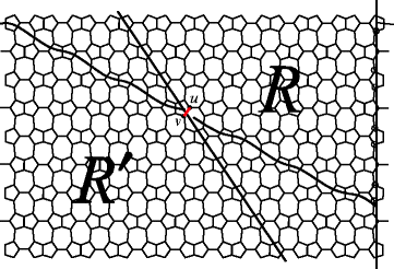

  

  $e=uv$ is an edge belonging to ${E_2}$ in $m=4\,\mathrm{th}$ row

  In Fig. 12.34, the vertices assigned by symbol $\circ$ have the same distance from $u$ and $v$. Then,

  • (i) If $m\leq A(-3)$ and $k-m\leq A(3)$, then

    $$ {b_1}={n_e}(u)=k\left( {2p+12m-6k-3} \right)-4{m^2}+2m-1-2C-2E. $$

  • (ii) If $A(-3)<m\leq \frac{p}{2}$ and $k-m\leq A(3)$, then

    $$ {b_2}={n_e}(u)=k(2p+12m-6k-3)-4{m^2}+2m-1-A(-3)-2E. $$

  • (iii) If $m>\frac{p}{2}$ and $k-m\leq A(3)$, then

    $$ \begin{array}{llll} {b_3}={n_e}(u)=k(2p+12m-6k-4)+m(4-6m+2p)\\ \quad -\frac{3}{2}{p^2}-\frac{1}{2}p-1-A(-3)-2E. \end{array} $$

  • (iv) If $m\leq A(-3)$ and $k-m>A(3)$, then

    $$ \begin{array}{llll} {b_4}={n_e}(u)=m(2p+2m-1)-1-2C+(2p-3)\times A(3)\\ \quad -6{(A(3))^2}-2A(3,1). \end{array} $$

  • (v) If $A(-3)<m\leq \frac{p}{2}$ and $k-m>A(3)$, then

    $$ \begin{array}{llll}{b_5}={n_e}(u)=m(2p+2m-1)-1+(2p-3)\times A(3)\\ \quad -6{(A(3))^2}-A(-3)-2A(3,1). \end{array} $$

  • (vi) If $m>\frac{p}{2}$ and $k-m>A(3)$, then

    $$ \begin{array}{llll} {b_6}={n_e}(u)=p\left( {2m+\frac{1}{2}p+1} \right)+(2p-3)\times A(3)\\ \quad -6{(A(3))^2}-A(-3)-2A(3,1). \end{array} $$

  And for ${n_e}(v)$, we have

  • (i) If $m\leq A(-3)$ and $k-m\leq \frac{p}{2}$, then

    $$ {b_7}={n_e}(v)=k(2p-4m+2k+1)-4{m^2}+2m-1. $$

  • (ii) If $m>A(-3)$ and $k-m\leq \frac{p}{2}$, then

    $$\begin{array}{llll} {b_8}={n_e}(v)=\left( {2p+1} \right)\left( {k-m} \right)+k\left( {2k-4m} \right)+2{m^2}+2p-4\\ \quad +\left( {2p-8} \right)\times A\left( {-3} \right)-6{{\left( {A\left( {-3} \right)} \right)}^2}-2A\left( {-3,0} \right). \end{array} $$

  • (iii) If $m\leq A(-3)$ and $k-m>\frac{p}{2}$, then

    $$ {b_9}={n_e}(v)=2p(2k-m)+3m-6{m^2}-\frac{1}{2}{p^2}+\frac{1}{2}p-1. $$

  • (iv) If $m>A(-3)$ and $k-m>\frac{p}{2}$, then

    $$ \begin{array}{llll}{b_{10 }}={n_e}(v)=4p(k-m)+\frac{5}{2}p-\frac{1}{2}{p^2}-4+(2p-8)\times A(-3)\\ \quad -6{(A(-3))^2}-2A(-3,0). \end{array} $$

• (g) If $e\in {E_3}$, then according to Fig. 12.35, the region $R$ has vertices that belong to ${N_1}\left( {\left. e \right|G} \right)$, and the region ${R}^{\prime}$ has vertices that belong to ${N_2}\left( {\left. e \right|G} \right)$.

  Fig. 12.35

  

  $e=uv$ is an edge belonging to ${E_3}$ in $m=4\,\mathrm{th}$ row

  In Fig. 12.35, the vertices assigned by symbol $*$ is closer to $u$, and the vertices assigned by symbol $\circ$ have the same distance from $u$ and $v$. Then,

  • (i) If $m\leq A(-5)$, then

    $$ {c_1}={n_e}(u)=m(2p+6m-1)-1+B. $$

  • (ii) If $m>A(-5)$, then

    $$ {c_2}={n_e}(u)=4pm-1+6{(A(-5))^2}-(2p+1)\times A(-5)+A(-5,0). $$

  And for ${n_e}(v)$, we have

  • (i) If $k-m\leq A(-5)$, then

    $$ {c_3}={n_e}(v)=k(2p-12m+6k-1)+m(6m-2p+1)-1-2E. $$

  • (ii) If $k-m>A(-5)$, then

    $$ {c_4}={n_e}(v)=4p(k-m)-1+6{(A(-5))^2}-(2p+1)\times A(-5)-2A(-5,0). $$

• (h) If $e\in {E_4}$, then,

  Fig. 12.36

  

  $e=uv$ is an edge belonging to ${E_4}$ in $m=4\,\mathrm{th}$ row

  according to Fig. 12.36, the region $R$ has vertices that belong to ${N_1}\left( {\left. e \right|G} \right)$, and the region ${R}^{\prime}$ has vertices that belong to ${N_2}\left( {\left. e \right|G} \right)$. Then,

  • (i) If $m\leq A(0)+1$, then

    $$ {d_1}={n_e}(u)=12m(m-1)+2-3C. $$

  • (ii) If $m>A(0)+1$, then

    $$ {d_2}={n_e}(u)=4pm-4p+2+12{(A(0))^2}+(12-4p)\times A(0)-3A(0,0). $$

  And for ${n_e}(v)$, we have

  • (i) If $k-m\leq A(0)$, then

    $$ {d_3}={n_e}(v)=12(k-m)(k-m+1)+2-3D. $$

  • (ii) If $k-m>A(0)+1$, then

    $$ {d_4}={n_e}(v)=4p(k-m)+2+12{(A(0))^2}+(12-4p)\times A(0)-3A(0,0). $$

• (i) If $e\in {E_5}$, then according to Fig. 12.37, the region $R$ has vertices that belong to ${N_1}\left( {\left. e \right|G} \right)$, and the region ${R}^{\prime}$ has vertices that belong to ${N_2}\left( {\left. e \right|G} \right)$. Then,

  $$ {e_0}={n_e}(u)={n_e}(v)=4pk-1-2(E+B). $$

Fig. 12.37

$e=uv$ is an edge belonging to ${E_5}$ in $m=4\,\mathrm{th}$ row

For simplicity, we define

• ${S_0}=\sum\limits_{m=1}^k {\left\{ {2p\left( {{a_1}{a_2}+{b_1}{b_7}} \right)+\frac{p}{2}\left( {{d_1}{d_3}+{e_0}^2} \right)} \right\}}.$

• ${S_1}=p\left\{ {\sum\limits_{m=1}^{k-A(-5)-1 } {{c_1}{c_4}} +\sum\limits_{m=k-A(-5)}^{A(-5) } {{c_1}{c_3}} +\sum\limits_{m=A(-5)+1}^{k-1 } {{c_2}{c_3}} } \right\}.$

• ${S_2}=p\left\{ {\sum\limits_{m=1}^{A(-5) } {{c_1}{c_4}} +\sum\limits_{m=A(-5)+1}^{k-A(-5)-1 } {{c_2}{c_4}} +\sum\limits_{m=k-A(-5)}^{k-1 } {{c_2}{c_3}} } \right\}.$

• ${S_3}=2p\left\{ {\sum\limits_{m=1}^{k-A(3)-1 } {{b_4}{b_7}} +\sum\limits_{m=k-A(3)}^{A(3) } {{b_1}{b_7}} +\sum\limits_{m=A(3)+1}^k {{b_2}{b_8}} } \right\}.$

• ${S_4}=2p\left\{ {\sum\limits_{m=1}^{A(-3) } {{b_4}{b_7}} +\sum\limits_{m=A(-3)+1}^{k-A(3)-1 } {{b_5}{b_8}} +\sum\limits_{m=k-A(3)}^k {{b_2}{b_8}} } \right\}.$

• $\begin{array}{llll} {S_5}=2p\left\{ \sum\limits_{i=1}^{{k-\frac{p}{2}-1}} {{b_4}{b_9}} +\sum\limits_{{m=k-\frac{p}{2}}}^{A(-3) } {{b_4}{b_7}} +\sum\limits_{m=A(-3)+1}^{k-A(3)-1 } {{b_5}{b_8}} +\sum\limits_{m=k-A(3)}^{{\frac{p}{2}}} {{b_2}{b_8}}\right. \\ \quad \left.+\sum\limits_{{m=\frac{p}{2}+1}}^k {{b_3}{b_8}} \right\}. \end{array}$

• $\begin{array}{llll} {S_6}=2p\left\{ \sum\limits_{m=1}^{A(-3) } {{b_4}{b_9}} +\sum\limits_{m=A(-3)+1}^{{k-\frac{p}{2}-1}} {{b_5}{b_{10 }}} +\sum\limits_{{m=k-\frac{p}{2}}}^{{\frac{p}{2}}} {{b_5}{b_8}} +\sum\limits_{{m=\frac{p}{2}+1}}^{k-A(3)-1 } {{b_6}{b_8}} \right.\\ \quad \left.+\sum\limits_{m=k-A(3)}^k {{b_3}{b_8}} \right\}. \end{array}$

• ${S_7}=\frac{p}{2}\left\{ {\sum\limits_{m=1}^{k-A(0)-1 } {{d_1}{d_4}} +\sum\limits_{m=k-A(0)}^{A(0) } {{d_1}{d_3}} +\sum\limits_{m=A(0)+1}^k {{d_2}{d_3}} } \right\}.$

• ${S_8}=\frac{p}{2}\left\{ {\sum\limits_{m=1}^{A(0) } {{d_1}{d_4}} +\sum\limits_{m=A(0)+1}^{k-A(0)-1 } {{d_2}{d_4}} +\sum\limits_{m=k-A(0)}^{k-1 } {{d_2}{d_3}} } \right\}.$

• ${S_9}=\sum\limits_{m=1}^k {\left( {2p{a_1}{a_3}+\frac{p}{2}{e_0}^2} \right)}.$

• ${S_{10 }}=2p\left\{ {\sum\limits_{m=1}^{{k-\frac{p}{2}-1}} {{a_1}{a_4}} +\sum\limits_{{m=k-\frac{p}{2}}}^k {{a_1}{a_3}} } \right\}.$

• ${S_{11 }}=2p\left( {\sum\limits_{m=1}^{{\frac{p}{2}}} {{a_1}{a_4}} +\sum\limits_{{m=\frac{p}{2}+1}}^{{k-\frac{p}{2}-1}} {{a_2}{a_4}} +\sum\limits_{{m=k-\frac{p}{2}}}^k {{a_2}{a_3}} } \right).$

The Szeged index of $\mathrm{H}{{\mathrm{C}}_5}{{\mathrm{C}}_7}[r,\ p]$ nanotube is given as follows:

• If $k\leq A(-5)$, then

  $$ \mathrm{SZ}={S_0}+\sum\limits_{m=1}^{k-1 } {p{c_1}{c_3}}. $$

• If $A(-5)<k\leq A(-3)$, then

  $$ \mathrm{SZ}={S_1}+{S_0}. $$

• If $A(-3)<k\leq A(0)+1$, then

  $$ \mathrm{SZ}={S_9}+{S_3}+{S_1}+\sum\limits_{m=1}^k {\frac{p}{2}{d_1}{d_3}}. $$

• If $A(0)+1<k\leq 2A(-5)$, then

  $$ \mathrm{SZ}={S_9}+{S_7}+{S_1}+{S_3}. $$

• If $2A(-5)<k\leq A(3)+A(-3)$, then

  $$ \mathrm{SZ}={S_9}+{S_7}+{S_2}+{S_3}. $$

• If $A(3)+A(-3)<k\leq 2A(0)+1$, then

  $$ \mathrm{SZ}={S_9}+{S_7}+{S_4}+{S_2}. $$

• If $2A(0)+1<k\leq \frac{p}{2}$, then

  $$ \mathrm{SZ}={S_9}+{S_8}+{S_2}+{S_4}. $$

• If $\frac{p}{2}<k\leq \frac{p}{2}+A(-3)$, then

  $$ \mathrm{SZ}={S_{10 }}+{S_8}+{S_2}+{S_5}+\sum\limits_{m=1}^k {{e_0}^2}. $$

• If $\frac{p}{2}+A(-3)<k\leq p$, then

  $$ \mathrm{SZ}={S_{10 }}+{S_8}+{S_2}+{S_6}+\sum\limits_{m=1}^k {{e_0}^2}. $$

• If $k>p$, then

  $$ \mathrm{SZ}={S_{11 }}+{S_8}+{S_2}+{S_6}+\sum\limits_{m=1}^k {{e_0}^2}. $$

Therefore, the Szeged index of above nanotube is computed.

12.3.6 Computation of the Szeged Index of Armchair Polyhex Nanotube

In this part, we compute the Szeged index of Armchair Polyhex nanotube. This nanotube is denoted by $\mathrm{TUA}{{\mathrm{C}}_6}[p,k]$. We bring all details of the computation of the Szeged index of this nanotube, which have been published in Mahmiani et al. (2008).

According to Fig. 12.38, we denote the number of horizontal lines in one row by $p$, and the number of levels by $k$.

Fig. 12.38

Two-dimensional lattice of $\mathrm{TUA}{{\mathrm{C}}_6}[4,14]$ nanotube, $p=4,\,k=14$

Let $e$ be an arbitrary edge of nanotube. For computing the Szeged index of $T$, we assume two cases:

Case 1

$p$ is even.

Lemma 12.3.20

If e is a horizontal edge of $T$, then ${n_1}(e\left| G \right.){n_2}(e\left| G \right.)={p^2}{k^2}.$

Proof

Suppose that $e$ is a horizontal edge of $T$, for example, $e=uv$ in Fig. 12.39. In this figure, the region $R$ has vertices that belong to ${N_1}\left( {\left. e \right|G} \right)$, and the region ${R}^{\prime}$ has vertices that belong to ${N_2}\left( {\left. e \right|G} \right)$. So we have ${n_1}(e\left| G \right.)={n_2}(e\left| G \right.)=pk$; therefore, ${n_1}(e\left| G \right.){n_2}(e\left| G \right.)={p^2}{k^2}.$ By the symmetry of $\mathrm{TUA}{{\mathrm{C}}_6}[p,k]$ nanotube for every horizontal edge, the above relation is hold. ▄

Fig. 12.39

$e=uv$ is a horizontal edge in level $m=6$

For simplicity, we define $a=\left[ {\frac{k-m-1 }{2}} \right]$ and $b=\left[ {\frac{m-1 }{2}} \right]$.

Lemma 12.3.21

Suppose $p$ is even. If $e$ is an oblique edge in level m, then we have

• (i) If $m\leq p$ and $k-m\leq p$, then

  $$ \begin{array}{llll}{n_1}\left( {e\left| G \right.}\right)=p(k+m-1)+2b(5-2m+3b-p)+2a(k-m-a-2)\\ \quad +2k-6m+2.\end{array} $$

  (I)

• (ii) If $m\leq p$ and $k-m>p$, then

  $$ {n_1}\left( {e\left| G \right.} \right)=p(2k-1/2p-1)+2b(5-p+3b-2m)-4m+4. $$

  (II)

• (iii) If $m>p$ and $k-m\leq p$, then

  $$ {n_1}\left( {e|G} \right)=p\left( {k-m+1/2p} \right)+2a\left( {k-a-m-2} \right)+2\left( {k-m-1} \right). $$

  (III)

• (iv) If m > p and k − m > p, then

  $$ {n_1}\left( {e|G} \right)=2p\left( {k-m} \right)+2. $$

  (IV)

Proof

Let e be an oblique edge of $T$, for example, $e=uv$ in Fig. 12.40. In this figure, the region R has vertices that belong to ${N_1}\left( {\left. e \right|G} \right)$, and the region ${R}^{\prime}$ has vertices that belong to ${N_2}\left( {\left. e \right|G} \right)$.

Fig. 12.40

$e=uv$ is an oblique edge in level $m=6$

Number of vertices that are closer to u than to v are as follows: If m ≤ p and k − m ≤ p, then

$$ \begin{array}{llll} {n_1}\left( {e|G} \right)= p(k-m+1)+\sum\limits_{i=1}^a {(4i)} \\ \quad + \sum\limits_{i=1}^b {(2p-4i)+(k-m-2a-1)(2a+2)} \\ \quad +(m-2b-1)(2p-4b-4)\\ = p(k+m-1)+2b(5-2m+3b-p)+2a(k-m-a-2)\\ \quad +2k-6m+2. \end{array} $$

If m ≤ p and k − m ≤ p, then

$$ \begin{array}{llll} {n_1}\left( {e|G} \right)= p(2k-2m-p+2)+\sum\limits_{i=1}^{{\frac{(p-2) }{2}}} {(4i)} +\sum\limits_{i=1}^b {(2p-4i)} \\ \quad + (m-2b-1)(2p-4b-4) \\ = p(2k-1/2p-1)+2b(5-p+3b-2m)-4m+4. \end{array} $$

If m > p and k − m ≤ p, then

$$ \begin{array}{llll} {n_1}\left( {e|G} \right)= p(k-m+1)+\sum\limits_{i=1}^a {(4i)} +\sum\limits_{i=1}^{{\frac{p-2 }{2}}} {(2p-4i)} +(k-m-2a-1)\\ \quad (2a+2)+2 \\ = p(k-m+1/2p)+2a(k-a-m-2)+2(k-m-1). \end{array} $$

And if m > p and k − m > p, then

$$ {n_1}(e|G)=p(2k-2m-p+2)+\sum\limits_{i=1}^{{\frac{(p-2) }{2}}} {(4i)} +\sum\limits_{i=1}^{{\frac{(p-2) }{2}}} {(2p-4i)} +2=2\mathrm{p}(\mathrm{k}\hbox{-}\mathrm{m})+2. $$

By the symmetry of $\mathrm{TUA}{{\mathrm{C}}_6}[p,k]$ nanotube for every oblique edge, this relation is hold.▄

Remark 12.3.22

According to Fig. 12.40, let e be an oblique edge in level m, then

$$ {n_2}(e|G)=2pk-{n_1}(e|G). $$

Theorem 12.3.23

If p is even, then the Szeged index of $\mathit{TUA}{C_6}[p,k]$ nanotube is given as follows:

• 1. k is even.

  • (i) If $k\leq p$, then we have

    $$ \begin{array}{llll} \mathrm{Sz}(T)={p^3}(2{k^3}-{k^2}-k+2)+{p^2}({k^2}-2k)+p(-1/6{k^5}+1/3p{k^4}\\ \quad +1/3{k^3}-1/3{k^2}-2/3k). \end{array} $$

  • (ii) If $p<k\leq 2p$, then we have

    $$ \begin{array}{llll} \mathrm{Sz}(T)= {p^5}(91/12-31/3k)+{p^4}\left( {14/3{k^2}-22/3k-10/3} \right)\\ \quad +{p^3}\left( {2{k^3}+1/2{k^2}+4/3k-4/3} \right) \\ \quad + {p^2}\left( {11/3{k^3}-4{k^2}-2/3{k^4}-4/3k+2/15} \right) \\ \quad +p(-1/30{k^5}-7/12{k^4}+7/3{k^3}-5/3{k^2}-4/5k)+31/5{p^6}. \end{array} $$

  • (iii) If $k>2p$, then we have

    $$ \begin{array}{llll} \mathrm{Sz}(T)= p\left( {1/4{k^4}-1/5{k^5}+2/3{k^3}-22/15k} \right)+{p^2}\left( +1/3{k^4}\right.\\ &\left.\quad +2/3{k^3}+2/3{k^2}-14/3k+22/15 \right) \\ \quad + {p^3}\left( {-2{k^3}+5/2{k^2}-8/3k+8/3} \right)+{p^4}\left( {10{k^2}-6k-2/3} \right)\\ \quad +{p^5}\left( {91/12-31/3k} \right)+31/5{p^6}. \end{array} $$

• 2. k is odd.

  • (i) If $k\leq p$, then we have

    $$ \begin{array}{llll} \mathrm{Sz}(T)=p\left( {-1/6{k^5}+1/3{k^4}-2/3{k^3}-4/3{k^2}+5/6k+1} \right)\\ \quad +{p^2}\left( {2{k^2}-2} \right)+{p^3}\left( {2{k^3}-{k^2}-k+1} \right). \end{array} $$

  • (ii) If $p<k\leq 2p$, then we have

    $$ \begin{array}{llll} \mathrm{Sz}(T)= {p^3}\left( {2{k^3}+1/2{k^2}+13/3k+13/6} \right)+{p^4}\left( +14/3{k^2}-22/3k\right.\\ \quad \left.-7/3 \right)+ p\left( {{-}1/30{k^5}{-}1/12{k^4}+1/3{k^3}+5/6{k^2}{-}3/10k-3/4} \right) \\ \quad +{p^2}\left( {{-}2/3{k^4}+5/3{k^3}{-}13/3k+17/15} \right)+91/12{p^5}{+}31/5{p^6}. \end{array} $$

  • (iii) If $k>2p$, then we have

    $$ \begin{array}{llll} \mathrm{Sz}(T)= {p^3}\left( {-2{k^3}+5/2{k^2}-11/3k+1/6} \right)+{p^4}\left( {+10{k^2}-6k+1/3} \right)\\ \quad +31/5{p^6}{+} p\left( {{-}1/5{k^5}{+}1/4{k^4}{-}1/3{k^3}{-}1/2{k^2}+8/15k+1/4} \right) \\ \quad +{p^2}\left( {1/3{k^4}+2/3{k^3}+5/3{k^2}-8/3k+22/15} \right)\\ \quad +{p^5}\left( {-31/3k+91/12} \right). \end{array} $$

Case 2

p is odd.

Lemma 12.3.24

If e is an oblique edge in level m, then we have

• (i) If $m\leq p$ and $k-m\leq p$, then ${n_1}(e|G)=p(k+m-1)+2b(5-2m+3b-p)+2a(k-m-a-2)+2k-6m+2$.

• (ii) If $m\leq p$ and $k-m>p$, then ${n_1}(e|G)=p(2k-1/2p-1)+2b(5-p+3b-2m)+-4m+7/2$.

• (iii) If $m>p$ and $k-m\leq p$, then ${n_1}(e|G)=p(k+m-1/2p)-3/2+2a(k-m-a-2)+2(k-m)$.

• (iv) If $m>p$ and $k-m>p$, then ${n_1}(e|G)=2p(k-m)$.

Theorem 12.3.25

If p is odd, then the Szeged index of $\mathrm{TUA}{{\mathrm{C}}_6}[p,k]$ nanotube is given as follows:

• 1. k is even.

  • (i) If $k\leq p$, then we have

    $$ \begin{array}{llll} \mathrm{Sz}(T)={p^3}\left( {2{k^3}-{k^2}-k+2} \right)+p\left( -1/6{k^5}+1/3{k^4}+1/3{k^3}-1/3{k^2}\right.\\ \quad \left.-2/3k \right)+{p^2}\left( {{k^2}-2k} \right). \end{array} $$

  • (ii) If $p<k\leq 2p$, then we have

    $$ \begin{array}{llll} \mathrm{Sz}(T)= {p^3}\left( {2{k^3}+1/2{k^2}-26/3k-41/6} \right)+p\left( -1/30{k^5}-7/12{k^4}\right.\\ \quad \left.+2/3{k^3}+11/6{k^2}-17/15k-7/4 \right) +{p^2}\left( -2/3{k^4}+11/3{k^3}\right.\\ \quad \left.+2{k^2}-10/3k-128/15 \right)+{p^4}\left( {14/3{k^2}-22/3k+4/3} \right) \\ \quad +{p^5}\left( {91/12-31/3k} \right)+31/5p_6. \end{array} $$

  • (iii) If $k>2p$, then we have

    $$ \begin{array}{llll} \mathrm{Sz}(T)= {p^3}\left( {-2{k^3}+5/2{k^2}-26/3k+7/6} \right)+p\left( -1/5{k^5}+1/4{k^4}\right.\\ \quad \left.+1/2{k^2}-4/5k+1/4 \right) +{p^2}\left( 1/3{k^4}+2/3{k^3}+8/3{k^2}\right.\\ \quad \left.-8/3k-6/5 \right)+{p^4}\left( {10{k^2}-6k+4} \right) \\ \quad +{p^5}\left( {91/12-31/3k} \right)+31/5{p^6}. \end{array} $$

• 2. k is odd.

  • (i) If $k\leq p$, then we have

    $$ \begin{array}{llll} \mathrm{Sz}(T)={p^3}\left( {2{k^3}-{k^2}-k+1} \right)+p\left( -1/6{k^5}+1/3{k^4}-2/3{k^3}-4/3{k^2} \right.\\ \quad \left.+5/6k+1 \right)+2{p^2}\left( {{k^2}-1} \right). \end{array} $$

  • (ii) If $p<k\leq 2p$, then we have

    $$ \begin{array}{llll} \mathrm{Sz}(T)= {p^3}\left( {-2{k^3}-17/3k+1/2{k^2}-10/3} \right)+p\left( -1/30{k^5}-1/12{k^4}\right.\\ \quad \left.-4/3{k^3}-2/3{k^2}+41/30k \right)+{p^2}\left( -2/3{k^4}+5/3{k^3}+3{k^2}\right.\\ \quad \left.+11/3k-8/15 \right)+{p^4}\left( {14/3{k^2}-22/3k+7/3} \right) \\ \quad +{p^5}\left( {91/12-31/3k} \right)+31/5{p^6}. \end{array} $$

  • (iii) If $k>2p$, then we have

    $$ \begin{array}{llll} \mathrm{Sz}(T)= {p^3}\left( {-2{k^3}+5/2{k^2}-29/3k-4/3} \right)+p\left( -1/5{k^5}+1/4{k^4}\right.\\ \quad \left.-{k^3}+1/5k \right)+ {p^2}\left( {1/3{k^4}+2/3{k^3}+11/3{k^2}-2/3k-1/5} \right)\\ \quad +{p^4}\left( {10{k^2}-6k+5} \right) +{p^5}\left( {91/12-31/3k} \right)+31/5{p^6}. \end{array} $$

12.3.7 Computation of the Szeged Index of Nanotubes by a Different Method

In the previous parts, we computed the Szeged index of some nanotubes by a theoretical method. It takes a long time for computing the Szeged index of a graph theoretically, especially when the graph has many vertices. In this part, we give an algorithm in the base of GAP, which is faster than the direct implementation. We bring all details of this program published in Taherkhani et al. (2009) and Iranmanesh et al. (2008a).

We give an algorithm that enables us to compute the Szeged index of any graph. For this purpose, the following algorithm is presented:

• 1. We assign to any vertex one number.

• 2. We determine all of the adjacent vertices set of the vertex i, i∈V (G), and this set is denoted by N(i). The set of vertices that their distance to vertex i is equal to t(t ≥ 0) is denoted by ${D_{i,t }}$ and consider ${D_{i,0 }}=\{i\}$. Let $e=ij$ be an edge connecting the vertices i and j; then we have the following result:

  • (a)
    $$ V=\bigcup\nolimits_{{f\geq 0}} {{D_{i.t }},i\in V(\mathrm{G}).} $$
  • (b)
    $$ \left( {{D_{i,t }}|{D_{j,t }}} \right)\subseteq \left( {{D_{j,t-1 }}\bigcup {{D_{j,t+1 }}} } \right),t\geq 1. $$
  • (c)
    $$ \left( {{D_{i,t }}\bigcap {{D_{j,t-1 }}} } \right)\subseteq {N_2}(e|G)\,\mathrm{and}\,{D_{i,t }}\bigcap {{D_{j,t+1 }}} \subseteq {N_1}(e|G)t\geq 1. $$
  • (d)
    $$ \begin{array}{llll} &{{{\left( {{D_{i,1 }}\bigcup {\{i\}} } \right)}} \left/ {{\left( {{D_{j,1 }}\bigcup {\{j\}} } \right)}} \right.}\subseteq {N_1}\left( {e|G} \right)\,\mathrm{and}\,{{\left( {{D_{j,1 }}\bigcup {\{j\}} } \right)}}\\ \quad \left/ {{\left( {{D_{i,1 }}\bigcup {\{i\}} } \right)}} \right.\subseteq {N_2}\left( {e|G} \right). \end{array} $$

  According to the above relations, by determining ${D_{i.t }},t\geq 1$, we can obtain ${N_1}(e|G)$ and ${N_2}(e|G)$ for each edge e, and, therefore, the Szeged index of the graph G is computed. By continuing we obtain the ${D_{i.t }},t\geq 1$ for each vertex i.

• 3. The distance between vertex i and its adjacent vertices is equal to 1; therefore, ${D_{i,1 }}=N(i)$. For each $j\in {D_{i.t }},t\geq 1$, the distance between each vertex of set ${N(j) \left/ {{\left( {{D_{i,t }}\bigcup {{D_{i,t-1 }}} } \right)}} \right.}$ and the vertex i is equal to $t+1$; thus, we have

  $$ {D_{i,t+1 }}=\bigcup {_{{j\in {D_{i,t }}}}} {(N(j) \left/ {{\left( {{D_{i,t }}\bigcup {{D_{i,t-1 }}} } \right)}} \right.},t\geq 1. $$

  According to the above equation, we can obtain ${D_{i.t }},t\geq 2$ for each $i\in V(\mathrm{G})$.

• 4. In the start of the program, we set SZ equal to zero and T equal to an empty set. In the end of program, the value of SZ is equal to the Szeged index of the graph G. For each vertex i, $1\leq i\leq n$, and each vertex j in N(i), we determine ${N_1}(e|G)$ and ${N_2}(e|G)$ for edge $e=ij$, then add the values of ${n_1}(e|G).{n_1}(e|G)$ to SZ. Since the edge ji is equal to ij, we add the vertex i to T and continue this step for the vertex i + 1 and for each vertex in ${N(i+1) \left/ {T} \right.}$.

GAP stands for Groups, Algorithms, and Programming (Schonert et al. 1992). The name was chosen to reflect the aim of the system, which is group theoretical software for solving computational problems in group theory. The last years have seen a rapid spread of interest in the understanding, design, and even implementation of group theoretical algorithms. GAP software was constructed by GAP’s team in Aachen. We encourage the reader to consult Dabirian and Iranmanesh (2005) and Trinajstic (1992) for background materials and computational techniques related to applications of GAP in solving some problems in chemistry and biology. According to the above algorithm, we prepare a GAP program to compute the Szeged index of dendrimers ${T_{k,d }}$.

Example 12.3.26

The Wiener index of tree dendrimers, ${T_{k,d }},k\geq 1,d\geq 3$, is computed in Entringer et al. (1994) and Gutman et al. (1994). Since the Wiener and Szeged indices coincide on trees (Gutman 1994 and Karmarkar et al. 1997), the Szeged index of ${T_{k,d }}$ is equal to its Wiener index (Fig. 12.41).

Fig. 12.41

Molecular graphs of dendrimers ${T_{k,d }}$

The following results are obtained in Entringer et al. (1994) and Gutman et al. (1994).

For every d ≥ 3, the tree ${T_{k,d }}$ has order

$$ n\left( {{T_{k,d }}} \right)=1+\frac{d}{d-2}\left[ {{(d-1)^k}-1} \right] $$

and its Szeged index is equal to the Wiener index, that is,

$$\begin{array}{llll} \mathrm{Sz}\left( {{T_{k,d }}} \right)=W\left( {{T_{k,d }}} \right)=\frac{1}{{{(d-2)^3}}}\left[ {(d-1)^{2k }}\left[ {k{d^3}-2(k+1){d^2}+d} \right]\right.\\ \quad \left.+2{d^2}{(d-1)^k}-d \right]. \end{array} $$

For computing of the Szeged index of ${T_{k,d }}$ by the above program, at first we assign to any vertex one number; according to this numbering, the set of adjacent vertices to each vertex, 1 ≤ i ≤ n, is obtained by the following program (part 1). In fact, part 1 of the program is the presentation of the graph. We use part 2 for computing the Szeged index of the graph.

The following program computes the Szeged index of the ${T_{k,d }}$ for arbitrary values of d and k.

d:=3; k:=3;#(For example)

n:=1+(d/(d-2) )*((d-1)^k - 1);

N:=[];

K1:=[2..d+1];

N[1]:=K1;

for i in K1 do

 if k=1 then N[i]:=[1];

  else

  N[i]:=[(d-1)*i+4-d..(d-1)*i+2];

 Add(N[i],1);fi;

od;

K2:=[d+2..1+(d/(d-2) )*((d-1)^(k-1) - 1)];

for i in K2 do

 N[i]:=[(d-1)*i+4-d..(d-1)*i+2];

 Add(N[i],Int((i-4+d)/(d-1)));

od;

K3:=[2+(d/(d-2) )*((d-1)^(k-1) - 1)..n];

for i in K3 do

 if k=1 then N[i]:=[1];

  else

 N[i]:=[Int((i-4+d)/(d-1))]; fi;

od;

# (Part2)

D:=[];

for i in [1..n] do

   D[i]:=[];

   u:=[i];

   D[i][1]:=N[i];

   u:=Union(u,D[i][1]);

   s:=1;

   t:=1;

   while s<>0 do

     D[i][t+1]:=[];

     for j in D[i][t] do

       for m in Difference(N[j],u) do

         AddSet(D[i][t+1],m);

       od;

     od;

   u:=Union(u,D[i][t+1]);

       if D[i][t+1]=[] then

      s:=0;

   fi;

   t:=t+1;

   od;

od;

T:=[];

sz:=0;

pi:=0;

for i in [1..n-1] do

N1:=[];

  for j in Difference(N[i],T) do

N2:=[];

    N1[j]:=Union(Difference(N[i],Union([j],N[j])),[i]);

    N2[i]:=Union(Difference(N[j],Union([i],N[i])),[j]);

      for t in [2..Size(D[i])-1] do

        for x in Difference(D[i][t],Union(D[j][t],[j])) do

          if not x in D[j][t-1] then

             AddSet(N1[j],x);

           elif x in D[j][t-1] then

            AddSet(N2[i],x);

         fi;

        od;

od;

   sz:=sz+Size(N1[j])*Size(N2[i]);

     od;

  Add(T,i);

od;

sz;# (The value of sz is equal to Szeged index of the graph)

Now, as an example, we compute the Szeged index of VC₅C₇[p,q] nanotube by GAP program.

A C₅C₇ net is a trivalent decoration made by alternating C₅ and C₇. It can cover either a cylinder or a torus nanotube (Fig. 12.42).

Fig. 12.42

VC₅C₇ [4, 2] nanotube

We denote the number of pentagons in the first row by p. In this nanotube, the first four rows of vertices and edges are repeated alternatively; we denote the number of this repetition by q. In each period, there are 16p vertices and 3p vertices which are joined to the end of the graph, and, hence, the number of vertices in this nanotube is equal to 16pq + 3p.

We partition the vertices of the graph to the following sets:

• K ₁: The vertices of the first row whose number is 6p.

• K ₂: The vertices of the first row in each period except the first one whose number is

  6p(q − 1).

• K ₃: The vertices of the second row in each period whose number is 2pq.

• K ₄: The vertices of the third row in each period whose number is 6pq.

• K ₅: The vertices of the fourth row in each period whose number is 2pq.

• K ₆: The last vertices of the graph whose number is 3p.

Figure 12.43 shows the rows of the mth period.

Fig. 12.43

The rows of mth period VC₅C₇[p,q] nanotube

We write a program to obtain the adjacent vertices set to each vertex in the sets K _i , i = 1…6. We can obtain the adjacent vertices set to each vertex by joining these programs. In this program, the value of x is the assigned number of vertex i in that row.

The following program computes the Szeged index of $\mathrm{V}{{\mathrm{C}}_5}{{\mathrm{C}}_7}\left[ {p,q} \right]$ nanotube for arbitrary p and q.

p:=4; q:=2; # (for example)

n:=16*p*q+3*p;

N:=[];

K1:=[1..6*p];

V1:=[2..6*p -1];

for i in V1 do

 if i mod 6=1 then N[i]:=[i-1,i+1,i+8*p];

  elif i mod 6 in [0,2,4] then N[i]:=[i-1,i+1];

   elif i mod 6=3 then N[i]:=[i-1,i+1,(1/3)*(i-3)+6*p+1];

    elif i mod 6=5 then N[i]:=[i-1,i+1,(1/3)*(i-5)+6*p +2];fi;

 N[1]:=[2,6*p,8*p+1];

 N[6*p]:=[6*p-1,1];

od;

K:=[6*p+1..16*p*q];

K2:=Filtered(K,i->i mod (16*p) in [1..6*p]);

for i in K2 do

 x:= i mod (16*p);

 if x mod 6=1 then N[i]:=[i-1,i+1,i+8*p];

  elif x mod 6=2 then N[i]:=[i-1,i+1,(1/3)*(x-2)+2+i-x-2*p];

   elif x mod 6=3 then N[i]:=[i-1,i+1,(1/3)*(x-3)+1+i-x+6*p];

    elif x mod 6=4 then N[i]:=[i-1,i+1,i-8*p];

     elif x mod 6=5 then N[i]:=[i-1,i+1,(1/3)*(x-5) +2+i-x+6*p];

      elif x mod 6=0 then N[i]:=[i-1,i+1,(1/3)*x +1+i-x-2*p];fi;

 if x=1 then N[i]:=[i+1,i-1+6*p,i+8*p];fi;

 if x=6*p then N[i]:=[i-1,i- 6*p+1,i- 8*p+1];fi;

od;

K3:=Filtered(K,i->i mod (16*p) in [6*p+1..8*p]);

for i in K3 do

 x:=(i-6*p) mod (16*p);

 if x mod 2=0 then N[i]:=[i-1,3*(x-2)+5+i-x- 6*p,3*(x-2)+5+i-x+2*p];

   else N[i]:=[i+1,2*x+i- 6*p,2*x+i+2*p];fi;

od;

K4:=Filtered(K,i->i mod (16*p) in [8*p+1..14*p]);

for i in K4 do

 x:=(i- 8*p) mod (16*p);

 if x mod 6=1 then N[i]:=[i-1,i+1,i- 8*p];

  elif x mod 6=2 then N[i]:=[i-1,i+1,(1/3)*(x-2)+2+i-x+6*p];

   elif x mod 6=3 then N[i]:=[i-1,i+1,(1/3)*(x-3)+1+i-x-2*p];

    elif x mod 6=4 then N[i]:=[i-1,i+1,i+8*p];

     elif x mod 6=5 then N[i]:=[i-1,i+1,(1/3)*(x-5)+2+i-x- 2*p];

      elif x mod 6=0 then N[i]:=[i-1,i+1,(1/3)*x+1+i-x+6*p];fi;

 if x=1 then N[i]:=[i-8*p,i+1,i+6*p-1];fi;

 if x=6*p then N[i]:=[i-1,i-6*p+1,i+1];fi;

od;

K5:=Filtered(K,i->i mod (16*p) in Union([14*p+1..16*p-1],[0]));

for i in K5 do

 x:=(i-14*p) mod (16*p);

 if x mod 2=1 then N[i]:=[i+1,3*(x-1)+i-x-6*p,3*(x-1)+i-x+2*p];

  else N[i]:=[i-1,3*(x-2)+2+i-x-6*p,3*(x-2)+2+i-x+2*p];fi;

 if x=1 then N[i]:=[i+1,i-1,i-1+8*p];fi;

 if x=2*p then N[i]:=[i-1,3*(x-2)+2+i-x-6*p,3*(x-2)+2+i-x+2*p];fi;

od;

K6:=[16*p*q+1..n];

for i in K6 do

 x:=i mod (16*p);

 if x mod 3=1 then y:= (2/3)*(x-1)+2+i-x- 2*p;

  elif x mod 3=2 then y:=i+x- 8*p;

   elif x mod 3=0 then y:=(2/3)*(x- 3)+3+i-x-2*p;fi;

if x=3*p then y:=i- 5*p+1;fi;

 N[i]:=[y];

 N[y][3]:=i;

od;

D:=[];

for i in [1..n] do

   D[i]:=[];

   u:=[i];

   D[i][1]:=N[i];

   u:=Union(u,D[i][1]);

   s:=1;

   t:=1;

   while s<>0 do

     D[i][t+1]:=[];

     for j in D[i][t] do

       for m in Difference(N[j],u) do

         AddSet(D[i][t+1],m);

       od;

     od;

   u:=Union(u,D[i][t+1]);

       if D[i][t+1]=[] then

      s:=0;

   fi;

   t:=t+1;

   od;

od;

T:=[];

sz:=0;

for i in [1..n-1] do

N1:=[];

  for j in Difference(N[i],T) do

N2:=[];

    N1[j]:=Union(Difference(N[i],Union([j],N[j])),[i]);

    N2[i]:=Union(Difference(N[j],Union([i],N[i])),[j]);

      for t in [2..Size(D[i])-1] do

        for x in Difference(D[i][t],Union(D[j][t],[j])) do

          if not x in D[j][t-1] then

             AddSet(N1[j],x);

           elif x in D[j][t-1] then

             AddSet(N2[i],x);

         fi;

        od;

     od;

   sz:=sz+ Size(N1[j])*Size(N2[i]);

  od;

  Add(T,i);

od;

sz; # (The value of sz is equal to Szeged index of the graph)

Also, as another example, we compute the Szeged index of $\mathrm{H}{{\mathrm{C}}_5}{{\mathrm{C}}_7}\left[ {p,q} \right]$ nanotube similar to the previous section. We computed the Szeged index of this nanotube in Sect. 12.3.5 by a theoretical method. A $\mathrm{H}{{\mathrm{C}}_5}{{\mathrm{C}}_7}\left[ {p,q} \right]$ nanotube consists of heptagon, pentagon nets as below (Fig. 12.44).

Fig. 12.44

HC₅C₇ [4,2] nanotube

We denote the number of heptagons in the first row by p. In this nanotube, the four first rows of vertices and edges are repeated alternatively; we denote the number of this repetition by q. In each period, 16p vertices and 2p vertices are joined to the end of the graph, and hence the number of vertices in this nanotube is equal to 16pq + 2p.

The following program is the same as the last program. In this program, value of x is the number of vertex i in a row.

p:=6;q:=7;# (for example)

n:=16*p*q+2*p;

N:=[];

for i in [1..5*p] do

 if i mod 5=1 then N[i]:=[i-1,i+1,(3/5)*(i-1)+1+5*p];

  elif i mod 5 in [0,2] then N[i]:=[i-1,i+1];

   elif i mod 5=3 then N[i]:=[i-1,i+1,(3/5)*(i-3)+2+5*p];

    elif i mod 5=4 then N[i]:=[i-1,i+1,(3/5)*(i-4)+3+5*p];fi;

 N[1]:=[2,5*p,5*p+1];

 N[5*p]:=[1,5*p-1];

od;

K:=[5*p+1..16*p*q];

K1:=Filtered(K,i->i mod (16*p) in [1..5*p]);

for i in K1 do

 x:=(i) mod (16*p);

 if x mod 5=1 then N[i]:=[i-1,i+1,(3/5)*(x-1)+1+i-x+5*p];

  elif x mod 5=2 then N[i]:=[i-1,i+1,(3/5)*(x-2)+1+i-x-3*p];

   elif x mod 5=3 then N[i]:=[i-1,i+1,(3/5)*(x-3)+2+i-x+5*p];

    elif x mod 5=4 then N[i]:=[i-1,i+1,(3/5)*(x-4)+3+i-x+5*p];

     elif x mod 5=0 then N[i]:=[i-1,i+1,(3/5)*x+i-x-3*p];fi;

 if x=1 then N[i]:=[i+1,i-1+5*p,i+(5*p)];fi;

 if x=5*p then N[i]:=[i-1,i-5*p,i+1-5*p];fi;

od;

K2:=Filtered(K,i->i mod (16*p) in[5*p+1..8*p]);

for i in K2 do

 x:=(i- 5*p) mod (16*p);

 if x mod 3 =1 then N[i]:=[i-1,i+1,(5/3)*(x-1)+1+i-x- 5*p];

  elif x mod 3 =2 then N[i]:=[i-1,(5/3)*(x-2)+3+i-x- 5*p,(5/3)*(x-2)+3+i-x+3*p];

   elif x mod 3 =0 then N[i]:=[i+1,(5/3)*x-1+i-x- 5*p,(5/3)*x +i-x+3*p];fi;

 if x=3*p then N[i]:=[i-3*p+1,(5/3)*x-1+i-x- 5*p,(5/3)*x +i-x+3*p];fi;

 if x=1 then N[i]:=[i-5*p,i+1,i-1+3*p];fi;

od;

K3:=Filtered(K,i->i mod (16*p) in [8*p+1..13*p]);

for i in K3 do

 x:=(i- 8*p) mod (16*p);

 if x mod 5=1 then N[i]:=[i-1,i+1,(3/5)*(x-1) +i-x+5*p] ;

   elif x mod 5=2 then N[i]:=[i-1,i+1,(3/5)*(x-2)+1+i-x+5*p];

    elif x mod 5=3 then N[i]:=[i-1,i+1,(3/5)*(x-3)+2+i-x-3*p];

     elif x mod 5=4 then N[i]:=[i-1,i+1,(3/5)*(x-4)+2+i-x+5*p];

      elif x mod 5=0 then N[i]:=[i-1,i+1,(3/5)*x +i-x-3*p];fi;

 if x=1 then N[i]:=[i+1,i-1+5*p,i-1+8*p];fi;

 if x=5*p then N[i]:=[i-1,i-5*p,i+1-5*p];fi;

od;

K4:=Filtered(K,i->i mod (16*p) in Union([13*p+1..16*p-1],[0]));

for i in K4 do

 x:=(i-13*p) mod (16*p);

 if x mod 3=1 then N[i]:=[i+1,(5/3)*(x-1)+2+i-x-5*p,(5/3)*(x-1)+2+i-x+3*p];

  elif x mod 3=2 then N[i]:=[i-1,i+1,(5/3)*(x-2)+4+i-x-5*p];

   elif x mod 3=0 then N[i]:=[i-1,(5/3)*x+1+i-x-5*p,(5/3)*x+i-x+3*p];fi;

 if x=3*p then N[i]:=[i-1,i+1-8*p,(5/3)*x+i-x+3*p]; fi;

od;

K5:=[16*p*q+1..n];

for i in K5 do

 x:=i mod(16*p);

 if x mod 2=0 then y:=(3/2)*x+i-x-3*p;

  else y:=(3/2)*(x-1)+1+i-x-3*p;fi;

 N[i]:=[y];

 N[y][3]:=i;

od;

D:=[];

for i in [1..n] do

   D[i]:=[];

   u:=[i];

   D[i][1]:=N[i];

   u:=Union(u,D[i][1]);

   s:=1;

   t:=1;

   while s<>0 do

     D[i][t+1]:=[];

     for j in D[i][t] do

       for m in Difference(N[j],u) do

         AddSet(D[i][t+1],m);

       od;

     od;

   u:=Union(u,D[i][t+1]);

       if D[i][t+1]=[] then

      s:=0;

   fi;

   t:=t+1;

   od;

od;

T:=[];

sz:=0;

for i in [1..n-1] do

N1:=[];

  for j in Difference(N[i],T) do

N2:=[];

    N1[j]:=Union(Difference(N[i],Union([j],N[j])),[i]);

    N2[i]:=Union(Difference(N[j],Union([i],N[i])),[j]);

      for t in [2..Size(D[i])-1] do

        for x in Difference(D[i][t],Union(D[j][t],[j])) do

          if not x in D[j][t-1] then

             AddSet(N1[j],x);

           elif x in D[j][t-1] then

            AddSet (N2[i],x);

         fi;

        od;

     od;

   sz:=sz+Size(N1[j])*Size(N2[i]);

  od;

  Add(T,i);

od;

sz;# (The value of sz is equal to Szeged index of the graph)

References

Agrawal VK, Bano S, Mathur KC, Khadikar PV (2000) Indian Acad Sci 112:137
Cameron P (1994) Combinatorics: topics, techniques, algorithms. Cambridge University Press, Cambridge
Dabirian M, Iranmanesh A (2005) MATCH Commun Math Comput Chem 54:75
Diudea MV, Stefu M, Parv B, John PE (2004) Croat Chem Acad 77:111
Entringer RC, Meir AJ, Moon W, Székely LA (1994) Australas J Combin 10:211
Gutman I (1994) Graph Theory Notes N Y 27:9
Gutman I, Yeh YN, Lee SL, Chen JC (1994) MATCH Commun Math Comput Chem 30:103
Holister CRV, Harper T (2003) Cientifica 6:1
Iranmanesh A, Gholami N (2007) Micro Nano Lett 4:107
Iranmanesh A, Gholami N (2008) Croat Chemica Acta 81:299
Iranmanesh A, Gholami N (2009) MATCH Commun Math Comput Chem 62:371
Iranmanesh A, Khormali O (2009) J Appl Sci 6:1670
Iranmanesh A, Pakravesh Y (2007) J Appl Sci 7:3606
Iranmanesh A, Pakravesh Y (2008) Utilitas Mathematica 75:89
Iranmanesh A, Soleimani B, Ahmadi A (2007) J Comput Thoer NanoSci 4:147
Iranmanesh A, Alizadeh Y, Taherkhani B (2008a) Int J Mol Sci 9:131
Iranmanesh A, Pakravesh Y, Mahmiani A (2008b) Ars Comb 87:193
Iranmanesh A, Gholami N, Ahmadi A (2010) Optoelectron Adv Mater Rapid Commun 4:2190
Karmarkar S, Joshi S, Das A, Khadikar PV (1997) J Serb Chem Soc 62:227
Mahmiani A, Iranmanesh A, Pakravesh Y (2008) Ars Comb 89:309
Mansoori GA (2005) Principles of nanotechnology: molecular-based study of condensed matter in small systems. World Scientific, Hackensack
Schonert M et al (1992) GAP, groups, algorithms and programming. Lehrstuhl De fu Mathematik, RWTH, Achen
Taherkhani B, Alizadeh Y, Iranmanesh A (2009) Asian J Chem 21:3683
Trinajstic N (1992) Chemical group theory. CRC Press, Boca Roton
Acknowledgments
This work was partially supported by Center of Excellence of Algebraic Hyperstructures and its Applications of Tarbiat Modares University (CEAHA).
Author information
Authors and Affiliations
Corresponding author
Editor information
Editors and Affiliations
Rights and permissions
Copyright information
© 2013 Springer Science+Business Media Dordrecht
About this chapter
Cite this chapter
Iranmanesh, A. (2013). Computation of the Szeged Index of Some Nanotubes and Dendrimers. In: Ashrafi, A., Cataldo, F., Iranmanesh, A., Ori, O. (eds) Topological Modelling of Nanostructures and Extended Systems. Carbon Materials: Chemistry and Physics, vol 7. Springer, Dordrecht. https://doi.org/10.1007/978-94-007-6413-2_12
Download citation
DOI: https://doi.org/10.1007/978-94-007-6413-2_12
Published:
Publisher Name: Springer, Dordrecht
Print ISBN: 978-94-007-6412-5
Online ISBN: 978-94-007-6413-2
eBook Packages: Chemistry and Materials ScienceChemistry and Material Science (R0)