Water Uptake and Water Supply

Abstract

The water uptake and the water supply do not directly affect the mineral absorption of plants. However, many connections exist between the management of minerals and water. The most evident of those connections are following

These keywords were added by machine and not by the authors. This process is experimental and the keywords may be updated as the learning algorithm improves.

6.1 Introduction

The water uptake and the water supply do not directly affect the mineral absorption of plants. However, many connections exist between the management of minerals and water. The most evident of those connections are the following.

• Water plays an important part with the transport of minerals in the root environment, thus, from surroundings to the root surface, and it is also important for the nutrient transport in the plant.

• The water management is also important with the vertical transport of salts in the root zone and with this for the leaching of residual salts and nutrients from the root zone to the deep ground water or surrounding surface water. Thus, it plays an important part in the operational efficiency of the management of minerals in greenhouse soils and substrates.

• The additions of nutrients in the greenhouse industry occur mainly with top dressings by fertigation, which means a combined addition of water and nutrients.

• Water often contain minerals, which partly can be estimated as residual salts, like Na and Cl, but for another part is appreciated as nutrients, like Ca, Mg, and SO₄, which directly affect the addition of nutrients in fertilization programmes. However, last group will be denoted as residuals when the concentrations in the irrigation water exceed those of the uptake concentrations.

• The ratio between the uptake of nutrients and water, denoted as uptake concentration, is used as a basis for nutrient supply. Despite, that the uptake concentration has no real physiological basis in the nutrition of plants, it offers valuable information. This because of the experience that the variations in the uptake concentrations are less than those of the absolute values of nutrient uptakes (Savvas and Lenz, 1995).

The factors mentioned are more than enough reasons to add a chapter about water supply to this book about plant nutrition. The water supply in the greenhouse industry is solely carried out by artificial irrigation and thus the control of it can easily be included in the management of the greenhouse. The water use and the water supply will not entirely be discussed in this chapter, but some guide lines in relation to the above mentioned factors will be presented.

6.2 Water Uptake by Plants

Water uptake by plants in greenhouses is entirely studied by Stanghellini (1987). In this study it was concluded that the transpiration rate is almost proportional to the leaf area and that in the greenhouse climate the radiation, the ambient temperature and the humidity play a prominent part. To a minor extent the temperature of the greenhouse cover and of the soil surface also play a part.

On basis of the factors affecting the water absorption of plants, models have been developed with simple and quickly measurable parameters. The stipulation that the parameters should be simple and quickly measurable is suggested by a practical suitability to irrigate on basis of the everyday water absorption of the crop. Nowadays, when many crops are grown in substrate systems, these requirements on the parameters are accentuated, because of the small water storage in the root environment of these systems and the need to keep this storage on a reasonable level. In such systems often water is supplied several times per hour and thus, the development of a method furnishing quick and preferably secure estimations of the water uptake are evident. Such estimations are developed by De Graaf (1988) on basis of the global radiation measured outside the greenhouse, the use of the heating system in the greenhouse, the air temperature in the greenhouse and the plant size. In formula (6.1) the relationship between the water uptake of the crop and the parameters mentioned is given.

$$E = \frac{h}{m}\left\{ a T_g R + b \mathop{\Sigma} \limits_{i = 1440}^{i = 1} {\rm{min}}_{i} (T_t - T_a )\right\}$$

((6.1))

In which

• E = estimated water uptake of the crop l m⁻² day⁻¹

• h = actual height or size of the crop

• m = minimum height or size of the crop with which the maximum transpiration can be realized. When h>m a value of 1.0 should be used for the quotient h/m

• a = emperical crop specific factor

• R = the global radiation measured outside the greenhouse in kJ cm⁻² day⁻¹

• T_g = the relative light transmission of the greenhouse

• b = specific crop factor attributable to heating

• min_i = the successive minutes during the day that there is a difference between the ambient temperature in the greenhouse and the heating tubes

• T_t = the temperature of the heating tubes

• T_a = the ambient temperature in the greenhouse

The water uptake as calculated with the formula presented can be divided into the part that is used by the plant for transpiration and the part that is used for plant growth. The last mentioned part is small in comparison with the first mentioned. In Fig. 6.1 the differences between both parts of the water uptake is shown as has been found for a tomato crop (Voogt et al., 2006b) for a period in early spring and a period in summer under Dutch conditions. Another part of water use is the evaporation from the soil and substrate surfaces. This only is of interest when soil and substrate surfaces are uncovered and especially when the whole soil surface regularly is irrigated, like with sprinkler irrigation and ebb and flow systems. This evaporation is often included in the measurements of the transpiration of the crop, because the water evaporated is added with the irrigation. It depends on the manner of the measurements whether the evaporation is included or excluded in the crop factor. Mostly the difference between the transpiration and the water use including the evaporation is small, like demonstrated by De Graaf and van den Ende (1981) and shown in Fig. 6.2.

Fig. 6.1

Typical daily pattern of the measured total water uptake, transpiration and plant growth of a tomato crop in g m⁻² h⁻¹, as affected by the radiation measured in W m⁻² over 5 minutes intervals, for a day in March (top) and a day in July (down). Both figures represent the averages of a period of 7 days. Results Voogt et al. (2006b)

Fig. 6.2

Cumulative water use during a soil grown tomato cropping, including the evaporation of the soil surface and the water uptake of the crop in l m⁻² (De Graaf and Van den Ende, 1981). Reprinted by permission of the International Society Horticultural Science

The advantage of the model presented affords the possibility of ad hoc applications by introduction of crop specific factors. Examples of crop specific factors are listed in Table 6.1. Most of these values are related to the global radiation measured outside the greenhouse. Therefore, the values are adjusted with light transmission of the greenhouse construction. These adjusted values will be used and the light transmission of the concerned greenhouse will be fit in the calculations, like done in formula (6.1). For the crop factor “b” attributed to the heating a value of 0.22 10⁻⁴ was found for tomato under Dutch growing conditions (De Graaf, 1988), while these factor also was used for cucumber (De Graaf and Esmeijer, 1998).

Table 6.1 Crop type factor “a” {M(a)} measured in a greenhouse with a light transmission (Tr_R) and related to global radiation measurements outside the greenhouse. The data are recalculated to a full light transmission in the greenhouse {C(a)}

The minimum plant height with which the maximum transpiration is realised, the factor m also will be known. This is a factor represented for the leaf area index (LAI), being an important factor in plant transpiration (Stanghellini, 1987). For practical application a plant is estimated as being mature with respect to the transpiration when LAI >3 (Voogt et al., 2006a). However, the LAI cannot be measured under growing conditions and therefore, is often estimated by the plant size. The actual plant size is related to the minimum size with maximum transpiration capacity. This value m in formula (6.1) is related to a certain plant height. For a row crop like tomato m is estimated on a height of 1.5 m. For crops with a high planting density, like chrysanthemum, a height of 0.25 m was suggested (De Graaf, 1993). However, Voogt et al. (2000) mentioned a height of 0.4 m for this crop in a more recent publication.

De Graaf (1988) supposed that addition of the results of measurements of the stoma resistance and the vapour pressure deficit should improve the estimation of the crop transpiration, like suggested by Stanghellini (1987) and Marcelis (1987). Therefore, Baas and Van Rijssel (2006) studied in an experiment the effect of different factors on the transpiration of a full grown rose crop. They measured the global radiation inside the greenhouse, the energy from heating under the canopy and the vapour pressure deficit (VPD_air and VPD_laef-air). They concluded that the transpiration can be estimated from the global radiation and the contribution of the heating and that the addition of the VPD_air or VPD_laef-air did not improve the estimation of the transpiration.

In modern greenhouses often artificial lighting and screening is applied. The screen can be a thermal screen used for energy saving which for the greater part transmit the light, or a full screen used for day length adjustment which exclude all radiation. In both cases the global radiation (R) must be corrected according to the screening time intervals and a specific reduction factor for the radiation of the actual screens. This factor (s_t in formula 6.2) is zero for the full screen. In case of artificial lighting the effective radiation also is taken into account. Therefore, the estimation of the transpiration by the model presented in formula (6.1) is modified. Voogt et al. (2006a) presented a formula for these adjustments, like shown in formula (6.2).

$$\begin{aligned}E =& \frac{h}{m}\left[ a\left\{ {T_g \left( {\mathop{\Sigma} \limits_{k = 1440}^{k = 1} \frac{\rm{min}_{k}}{{1440}}R + \mathop \Sigma \limits_{m = 1440}^{m = 1} \frac{{\rm{min}_{m} }}{{1440}}s_t R} \right) + \mathop \Sigma \limits_{n = 1440}^{n = 1} \frac{{\rm{min}_{n} }}{{1440}}R_a } \right\}\right.\\&\left. + b\mathop \Sigma \limits_{i = 1440}^{i = 1} \rm{min}_{i} (T_t - T_a ) \right]\end{aligned} $$

((6.2))

In which:

• min_k   = time that no screen in the greenhouse is used in min day^–1

• min_m   = time that only the thermal screen in the greenhouse is used in min day^–1

• min_n   = time that the artificial lighting is in operation in min day^–1

• s_t   = the relative light transmission of the screen in the greenhouse

• R_a   = effective radiation from artificial lighting during operation in kJ cm⁻² day⁻¹ as calculated from formula (6.2a)

• The other parameters as indicated with formula (6.1).

R_a can be calculated following installed (used) capacity (De Graaf and Spaans, 1998; De Graaf et al, 2004; Houter, 1996), following formula (6.2a).

$$R_a = 0.75\;P\;3.6\;h_a$$

((6.2a))

In which:

• R_a   = as indicated with formula (6.2)

• P  = installed capacity in W m⁻²

• h_a  = hours of operation

The formulae presented are based on optimal growing conditions concerning water supply, plant nutrition and climatic conditions in the greenhouse. However, some factors not mentioned in the formulae are well known as affecting the water use of greenhouse crops. The best known are salinity in the root environment and the CO₂ concentration of the air.

With respect of salinity the suppositions are often based on the misunderstanding that a low osmotic potential (high EC) in the root environment reduces the water uptake by plants. An abrupt increase of the salinity decreases the water absorption indeed (Van Ieperen, 1996), but over long periods big differences in water use of plants grown at different salinities have not necessarily been found, as long as the transpiration capacity, like for example the leaf area, is not strongly affected by the salinity. This has been found for tomato as shown in Table 6.2 (Sonneveld, 2000) and for radish (Sonneveld and Van den Bos, 1995). Despite that the yield of the tomato was significantly reduced by an increased EC in the root environment as shown in Table 6.2, the water absorption was not affected. Thus, the well known wilting after a heavy osmotic shock only occur for a short period and plants quickly adjust their water adsorption and will not show a further water stress. However, this does not alter the fact that in many cases a reduced water adsorption has been observed with increasing salinity (Baas et al., 1995; De Kreij and Van den Berg, 1990; Yaron et al., 1969). This is caused by adaptation of plants to salinity stress, like a reduction of the leaf area, and not directly by a hindrance of water absorption (Lagerwerff and Eagle, 1962).

Table 6.2 Water absorption of tomato plants grown at different EC values in a recirculation nutrient solution. The growing period was from June until September

With respect to increased CO₂ concentrations it has been found that the transpiration is affected only to a small extent, which under practical conditions was restricted to some percentages (Nederhof, 1994). Eggplant was most sensitive and showed periodical a reduction of 15% over certain periods, but over the whole growing season a reduction of 4% was calculated.

6.3 Variations of Uptake and Supply

Many different irrigation systems are available in the greenhouse industry. They can be globally distinguished in following groups.

• Systems due to spot or strip irrigation, like drip irrigation systems and mini sprinklers. This group is characterized by local wet spots or strips in the greenhouse where the water is supplied, while the remaining part of the surface stays dry. The crop is not wetted during irrigation (Van den Ende and De Graaf, 1974).

• Systems with which the whole area of the greenhouse is irrigated, like with high level sprinkler irrigation, see Picture 6.1. The spray lines with nozzles are placed in top of the greenhouse. The whole greenhouse area and also the crop canopy are wetted with any irrigation.

  

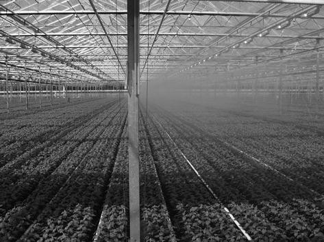
  Picture 6.1Irrigation by overhead sprinkling in a greenhouse with soil grown chrysanthemum

• Circulating systems, in which the water is continuously circulated in a thin layer, like in (NFT) nutrient film technique systems (Graves, 1983) or in thick layer, like in deep flow cultures (Maloupa, 2002). The plant grows directly in the water stream or water layer.

• Ebb and flow systems for plants grown in containers or in pre-shaped blocks. With these systems the water is supplied in a thin layer for a relatively short period. During this period, sufficient water is absorbed by the substrate and afterwards the system is drained. This system is often used for potted plants on tables and in gullies and for plant propagation on concrete floors.

The water uptake among individual plants varies strongly, as well as the local water supply of irrigation systems. This has been shown by studies of Van der Burg and Hamaker (1987) and of Van Schie et al. (1982) for drip irrigation systems. In the study of Van der Burg and Hamaker (1987) the water supply and the drainage water was measured on different spots in a greenhouse grown with tomato on rock wool slabs during a period from March until September. The spots measured held two tomato plants and both plants were supplied with a dripper. The average coefficient of variation of the water supply increased during the season from 4.8 till 13.2%, while the coefficient of variation of the water uptake was not increased during the season and on average amounted to 10.2%. Because the measured spots held two plants and thus, also two drippers, follow that for a single dripper or plant the coefficient of variation increases with a factor . This resulted in a value for the coefficient of variation from 6.8 till 18.7% for the water supply and 14.4% for the water uptake. The drainage water is affected by the variation of the uptake by the plant as well as by the variation of the supply. Those variations are independently and thus, the variation of the drainage water will be calculated as following formula (6.3).

$$s_d = \sqrt {s_s^2 + s_u^2 }$$

((6.3))

In which

• s_d  = the standard deviation of the drainage water

• s_s  = the standard deviation of the water supply

• s_u  = the standard deviation of the water uptake of the plant

Results of such calculations derived from the data in Fig. 6.3 are summarized in Table 6.3. Under practical conditions it can be supposed for example that a plant can use water from the plants left and right besides to compensate a possible shortage. In this case the coefficient of variation will be divided by a factor resulting from an average reaction of 3 plants together. Furthermore, plants will not suffer from drought, thus the drainage always will be ≥ 0. This will be approximated with a confidence limit of for example 1% (P ≤ 0.01), which means that on average not more than one on a hundred plants will suffer from drought. This agrees with a standard normal distributed unit T of 2.33. In this way the drainage will be calculated in relation to the water uptake by formula (6.4).

$$d \ge T\frac{{s_d }}{{\sqrt {p_n } }}$$

((6.4))

Fig. 6.3

Variation in water supply of drippers, water uptake by tomato plants grown in rock wool and drainage water as has been found on 32 sites in a greenhouse. The quantities are expressed as l m⁻². Data derived from Van der Burg and Hamaker (1987)

Table 6.3 Average values and variation, standard deviation (s) and coefficient of variation (cv), calculated from the data in Fig. 6.3 for the data measured at the spots of two plants and as estimated for a single plant. The water quantities are given as l m⁻² and l plant⁻¹ for the two plant spots and single plant situation, respectively

In which

• T  = standard normal distributed unit agreeing with a determined confidence limit

• d  = the quantity of drainage water, required as oversupply

• p_n  = the number of plants that can equalize the water mutually and the value mostly will vary between 1 and 3

• s_d  = standard deviation of the drainage water as given in formula (6.3)

In this formula s_d will be calculated from formula (6.3) in which s_s will be found by iteration, when the water uptake is determined. Calculations of the required drainage with formula (6.4) were carried out for a water uptake of 2 l, a vc_u = 10% and p_n values 1−3. The required oversupply can be expressed on the supply, like shown in Fig. 6.4, and this fraction is independent of the level of the supply. In Fig. 6.4 it is presented as the “inequality fraction”. The value strongly increases with the coefficient of variation of the irrigation system, especially in the single plant situation and soon reaches a value of 40%. This agrees well with experiences under practical conditions, because the coefficient of variation of drippers easily increases to values over 20% (Van Schie et al., 1982). The plant factor (p_n) depends on factors like the growing conditions and the plant age. Plants need time to adjust their root system on the water supply. For example, in the situation of a row crop with one nozzle per plant, in the beginning each plant is dependent of the water supply of the one nozzle placed near the plant. Later on when the root system extends, mutual utilization of the water supplied by three or possible more nozzles can be supposed.

Fig. 6.4

Inequality fraction as affected by the coefficient of variation of the drip system and the number of plants that mutually can profit from the water supplied. The confidence limit for the drainage water ≥ 0 is put on P = 0.01 and the coefficient of variation of the water uptake of the plant is put on 10%. See also the text

Variation in the water supply does not occur just with drip irrigation systems, but also were found with sprinkler irrigation systems. Sonneveld (1995) reported work of Heemskerk, in which the distribution of the water supply by sprinkler irrigation systems were measured on small sites with areas of 0.2 × 0.25 m. The coefficient of variation of the precipitation in the sites was 22%. In later measurements coefficients of variation for the water release of sprinkler installation up to 20% were common practice (Heemskerk et al., 1997). Thus, also with sprinkler irrigation systems an ample water supply is necessary to equalize effects of dry spots. Calculations in a model with an unequal distribution of the water supply of a sprinkler irrigation system for a chrysanthemum crop learned that with a coefficient of variation of the sprinkler irrigation system of 27% an overdose of water 22% is necessary to supply all plants sufficiently with water (Assinck and Heinen, 2001). This resulted to a leaching fraction of 20% of the water supplied, which is in good agreement with experiences in practice (Sonneveld, 1993b). A different option in the calculations of Assinck and Heinen was the addition of so much water, that nearly no leaching occur, with as a consequence that part of the plants suffer from drought. Last option mostly is not accepted for economic reasons in the greenhouse industry.

Besides the variation inherent in the design and the technical lay-out of the irrigation system, the unequal water distribution is strongly aggravated by clogging of drippers and nozzles. This clogging often is caused by precipitation of constituents from the primary water used and from the fertilizers added or from the growth of micro organisms. In an investigation the composition of precipitated materials was analysed from drippers of different greenhouse holdings in The Netherlands (De Bes, 1986). In the precipitated material substantial quantities of ortho-P, Ca, Fe, Al, Si, S and organic material were found, as follows from the data listed in Table 6.4. The origin of some constituent can be explained by the addition of fertilizers, like P and Ca. A combination of these elements easily precipitates at higher pH (> 6.5) values. Fe, Al and Si are highly represented in dust and clay particles, but Ca, Fe and Si are often available in primary water and can be a precipitate also from this origin. Organic matter can occur in the primary water, especially in surface water. This soluble organic matter will precipitate by changes of the pH or by addition of cations with the fertigation practices. In well water organic matter easily can occur by the development of bacteria. The growth of some specific species is strongly promoted by high methane concentrations sometimes found in this type of water (De Kreij et al., 2003). The bacterial slime build up in such cases also is traced as the cause for clogging and is determined in the analysis as organic material.

Table 6.4 Chemical composition of precipitated materials from drippers of different greenhouse holdings. Loss on ignition in % of the dry matter and elements as mol kg^{− 1} dried material. Where – is given the element was no substantial part of the precipitated materials

Logic components that occur in the precipitates in are Ca₃(PO₄)₂ or CaHPO₄ with possible equivalent compounds of Fe or Al, furthermore H₄SiO₄, Fe(OH)₃, Al(OH)₃ and CaSO₄, are likely. All compounds possible will precipitate together with crystalline water, which will be part of the loss on ignition determined. Sample nr 3 in Table 6.4 for example, clearly shows a precipitate of CaHPO₄ and sample nr 4 a precipitate of CaSO₄. The other samples existed of more complex components.

6.4 Water Quality

The quality of the irrigation water with respect to the mineral composition affects the water supply. When the concentration of any mineral is higher than the uptake concentration, the residual salt accumulates in the root environment and will be leached by extra water supply. Na and Cl are the ions often abundantly present in water, but sparingly absorbed by most greenhouse crops. Therefore, these ions often determine the leaching requirements. However, in specific cases other ions, like Ca, Mg or SO₄ also can control the need of leaching. In Table 7.13 some examples of the composition of irrigation water are listed in comparison with the uptake concentrations of minerals of two greenhouse crops.

Picture 6.2A basin for storage of rain water

Approximate concentrations for irrigation water with which it is possible to grow greenhouse crops without salt accumulation in the root environment are listed by Sonneveld (1993a). A review of such data is presented in Table 6.5. The precise concentrations acceptable for specific crops vary, because of the great differences in the uptake concentrations. For most crops Na is more critical than Cl, because of the lower uptake of this element by most crops. From data presented by Sonneveld (2000) for Na and Cl at low concentrations in the root environment (< 5 mmol l⁻¹) for Na a range can be given from virtually 0.0 mmol l⁻¹ for a rose crop until 1.8 mmol l⁻¹ for a winter grown radish crop. The value of 1.8 mmol l⁻¹ for winter grown radish is quite exceptional and connected with the low water uptake under Dutch climate conditions in winter. For most crops the uptake of Na and Cl is significantly increased at higher concentrations in the root environment, with exception of crops with a very low uptake, like rose. The uptake does not only differ among crops, but can differ also for cultivars, like shown in Fig. 6.5 for the uptake of Cl with alstroemeria (Sonneveld, 1988). The uptake also will be affected by the concentration of other ions. This is shown by the results of an iris crop grown on pumice and irrigated with water of a NaCl concentration of 8 mmol l⁻¹ (De Kreij and Van der Burg, 1998). Some data of this experiment are summarized in Table 6.6. The uptake of Na and Cl is much higher at a low fertilization level than at a standard fertilization, especially the transport of Na to the shoot is increased at low fertilization. The uptake concentration for Na was doubled, but as a result of the low fertilization the growth of the crop was strongly reduced. Comparable data are shown in Table 7.7 with bouvardia. The higher fertilization level reduced the Na uptake and thereby the toxic effect of the high sodium uptake. Often such effects merely are attributable to K uptake, which strongly aggravates or reduces the Na uptake with low or high K concentrations in the root environment, respectively; see also Satti et al. (1996). Comparable data has been found by changing of the Cl/NO₃ ratio with rock wool grown tomatoes (Voogt and Sonneveld, 2004), shown in Fig. 6.6. High Cl/NO₃ ratio went in hands with a low NO₃ concentration in the root environment, which strongly aggravated the uptake of Cl. Thus, extra uptake of Na and Cl can be realised by specific interventions in the fertilization. However, such interventions need very close control on the nutrient status in the root environment, because strong interventions in the nutrient status in the root environment easily induce yield reduction. Therefore, under practical growing conditions seldom uptake concentrations can be realised much higher than those presented in Table 6.5.

Fig. 6.5

Relationships between the Cl concentration in the root environment (mmol Cl l⁻¹ of the 1:2 volume extract) and the Cl concentration in the leaves (mmol kg ⁻¹ dry matter) for different alstroemeria cultivars grown in soil. Data after Sonneveld (1988)

Fig. 6.6

Cl uptake concentration as affected by the Cl/NO₃ ratio for rock wool grown tomato. Data after Voogt and Sonneveld (2004)

Table 6.5 Limits for ion concentrations in primary irrigation water whereby no accumulation of the ions mentioned occurs in the root environment

Table 6.6 Effects of the fertilization level on the uptake of Na and Cl by an iris crop, grown in pumice with irrigation water of a NaCl concentration of 8 mmol l⁻¹

The salinity status of a soil during cultivation often is strongly related to the water supply, like shown for a cucumber crop in Fig. 6.7. The EC of the saturation extract is followed during a whole growing season, together with the water supply. At start in winter a base fertilization is given and the water supply is low in that period. The EC in the root environment increases further on during the first period, because of sparingly water supply and salt accumulation from the deeper soil layers. In spring when the ample water supply is started the EC decreases by leaching of salts, because the water supply was 5–6 l m ⁻² day⁻¹, while the transpiration on average will be estimated on 2–3 l m⁻² day⁻¹. The EC decreases only until a certain required level and is maintained on that level later on by regular top dressings with nutrients. In substrate systems salt accumulation will occur quickly, because of the restricted root volume. Nice examples of salt accumulation are shown by Savvas et al. (2005a) in a closed hydroponics system grown with cucumber for 120 days. The NaCl concentration in the primary water used were 0.8, 5, 10 and 15 mmol l⁻¹ and after 120 days the concentrations in the drainage water were accumulated to about 8, 30, 45 and 55 mmol l⁻¹, respectively. The uptake concentration of Na and Cl increased significantly, but the high concentrations in the root environment ensure a substantial yield reduction of 12% per unit EC value measured in the drainage water (Savvas et al., 2005b). Such data underlines the need of leaching of salts by extra water supply during cultivation in substrate systems.

Fig. 6.7

Course of the EC of the saturation extract in the top soil (0.25 m) and the water supply in a greenhouse with soil grown cucumber. After Sonneveld (1969)

The leaching requirements will be calculated with formula (7.4). This formula is mainly based on the ion concentration in the primary water and this in the drainage water, supposing that the concentration added with the fertilizer application is under control and relatively low. Formula (7.4) can be applied for a specific salt as well for the EC as a measure for the total salt concentration. The concentration of the drainage water used in this formula reflects the concentration accepted as the maximum concentration in the drainage water or in the soil solution that leaves the root zone. The accumulation of salts depends much on the growing system, whereby the irrigation system plays a substantial part. With an overhead sprinkler system the whole area is irrigated and the salts will be washed down to deeper soil layers, or to a possible drainage system by which it is transported to the deep ground water and the surrounding surface water, respectively. With spot or strip irrigation part of the salts accumulate on the dry spots or paths during cultivation and at the end of the cropping period an unequal distribution of salts will occur. Local accumulations in the top layers between drippers also can occur in substrates when the surface of the substrate is not covered and furthermore, the accumulation follows its path to the drainage (Van Noordwijk and Raats, 1980). But even when substrates are wrapped in plastic bags, local accumulations can be substantial and will be highest in the end of the growing season (Van der Burg and Sonneveld, 1987). The measurements of the EC of the nutrient solution extracted from rock wool slabs in greenhouses under such conditions varied between values of about 2.5 and 8.0 dS m⁻¹. Salt accumulations in the root zone belong to growing systems under practical conditions in greenhouses, it is more or less impossible to prevent it and it is strongly promoted by a local supply of the irrigation water (Heinen, 1997), like also shown in Fig. 6.8 (Voogt and Van Winkel, 2009). The salt accumulation shows a contradictory pattern with the moisture content and the EC in the 1:2 volume extract varies from about 0.5 till 4.0 dS m⁻¹, which can be calculated to 2.4–13.3 in the soil solution. It can be expected that the differences in soils generally will be of the same size as found with substrates.

Fig. 6.8

The two dimensional pattern of EC (1:2 volume extract) and volumetric moisture content distribution in the soil profile with tomato irrigated with drip irrigation, determined longitudinal and in soil layers of 12.5 cm depth, determined halfway and at the end of a long term tomato cropping (after Voogt and Van Winkel, 2009)

The leaching requirements as mentioned before and calculated with formula (7.4) are operative for soil as well substrate growing. The management during crop cultivation is already discussed in Section 7.9, but can differ for substrate and soil growing. The main difference between soil and substrate is the root volume in which the plant is grown. The small volumes used in substrate growing on the one hand accentuate the need of leaching during cultivation, but on the other hand it opens excellent possibilities to control the salinity status.

Beside the leaching requirements during cultivation to prevent too high salt accumulations in the rooting zone, for soil grown crops leaching of accumulated salts can be necessary before starting a new crop. The need for this leaching not only depends on the accumulated salt concentration, but also on the consecutive crops. When a crop ends with a very unequal distribution of salts in the soil profile and the next crop covers the whole area of the greenhouse with a high planting density, an intensive flooding is necessary to prevent an unequal start of the next crop. This for instance is the case in crop rotations of fruit vegetables followed by leafy vegetables, radish and a lot flower crops. When in crop rotation comparable crops are succeeding, like fruit vegetable in rows, at the start a somewhat higher salinity status of the soil is often desirable and a heavy flooding is not necessary.

The flooding of soils is based on the replacement of the soil solution by fresh water and movement of the actual soil solution out of the root zone. The quantity of water required to that purpose depends on the depth of the root zone, the water holding capacity of the soil and the dispersion factor. This dispersion factor depends on the soil type and is high for soils with a course granule structure, like clayey soils. The quantity of water necessary for leaching can be calculated by the formula (6.5).

$$wv_l = wv_f f_d d$$

((6.5))

In which

• wv_l  = water necessary for flooding in mm

• wv_f  = volume fraction of water of the soil at field capacity as defined in formula (3.6)

• f_d  = dispersion factor

• d  = depth of the soil layer that will be washed out in mm

The Dutch advisory service maintained for the soils used in the greenhouse industry dispersion coefficients varying from 1.25 to 2.0 for sandy and clayey soils, respectively. Some results of their calculations used as recommendations for growers are summarized in Table 6.7 (Van den Bos et al., 1999).

Table 6.7 Water quantities required for leaching (wv_l) of a greenhouse soil over a depth of 250 mm, dependent on soil type, volume fraction of water at field capacity (wv_f) and dispersion factor (f_d)

In some well water under anaerobic conditions soluble Fe is present as bivalent Fe ions, which can be harmful to plants. This bivalent Fe easily oxidizes to trivalent Fe, when the water comes into contact with O₂. This process can be simply quickened by aeration or chemical oxidation systems (Ten Cate, 1978). The trivalent Fe precipitate as Fe(OH)₃. The chemical reaction is presented in formula (6.6).

$$4Fe^{2 + } + O_2 + 18H_2 O \to 4Fe(OH)_3 \downarrow + 8H_3 0^ +$$

((6.6))

With the oxidation H₃O ions are released, as follows from formula (6.6). This can be responsible for a strong decrease of the pH in the water under treatment, followed by a retardation of the oxidation process. Therefore it is important that the pH of the water is sufficiently buffered, to react with the released H₃O ions. The pH buffer when available in well water mainly exists of HCO₃. When the Fe is oxidized, a good filtration is necessary to separate the precipitated Fe from the water. In Fig. 6.9 effects of irrigation water with overhead spraying on plants are shown in relation to the HCO₃ concentration and the soluble Fe concentration in the irrigation water (Van den Ende, 1970). Despites, soluble Fe is not highly toxic to plants, it has different drawbacks when the concentrations pass certain thresholds. Summarizing, following situations will occur, when the irrigation water contain substantial concentrations of soluble Fe.

• Leaf scorching when sprayed over the crop, which especially occur when the Fe can be insufficiently oxidized. For limits see Fig. 6.9

• Contamination of greenhouse construction, crops and harvested produce when used for overhead spraying. The limits are denoted in Fig. 6.9

• Clogging of irrigation systems as mentioned in Section 6.3. This occurs with all Fe soluble in primarily irrigation water and the clogging get worse with increasing concentrations.

Fig. 6.9

Effects of soluble Fe (μmol l⁻¹) in the irrigation water on crops when used for overhead spraying in relation to the HCO₃ concentration (mmol l⁻¹). After van den Ende (1970)

See also Section 7.8 about effects of Fe in irrigation water.

6.5 Water Supply

The water supply during crop cultivation ultimately results from three main factors being:

• The uptake of the crop and the evaporation of the surface as discussed in Section 6.2

• The inequality resulted from differences by the plant uptake as well as by the distribution of the irrigation system as discussed in Section 6.3

• The leaching requirements determined by the water quality and the accepted salt accumulation in the root zone, as discussed in Section 6.4 and will be calculated by formula (7.4)

Thus, the water supply during cultivation can be formulated as follows in formula (6.7).

$$S_w = \frac{E}{{(1 - I)(1 - LF)}}$$

((6.7))

In which

• S_w  = water supply

• E  = estimated transpiration of the crop as denoted in the formulae (6.1) and (6.2)

• I  = inequality factor as discussed in Section 6.3 and calculated with the aid of formula (6.4)

• LF  = leaching fraction as discussed in Section 6.4

The inequality factor and the leaching fraction are multiplied in formula (6.7), because both factors are mutually independent.

Despite the reliable relationships found between the water uptake of plants and the different explaining climatic factors, under practical conditions serious errors occur, like shown in Fig. 6.10. The reason of such errors will be explained by different minor factors as presented by De Graaf (1995) and inaccuracies and deviations of the models developed. Such errors especially in substrate systems easily can deregulate the water management, because of the small water storage available in the root environment. Therefore, for substrate grown crops a system for water supply has been developed with a feed back on the amount of drainage water (De Graaf, 1988). To this purpose the amount of drainage water will be measured and dependent on the results the estimated water requirement is adjusted. With frequent irrigations, like often occur with substrate growing, the length of the interval between the irrigation periods is adjusted. With less frequent irrigations better the length of the irrigation period can be adjusted.

Fig. 6.10

Water uptakes in relation to the global radiation of rock wool grown tomato during two days in April. The water uptake was calculated following the model after Voogt et al. (2006b) and measured with an automatic balance. On the left a good agreement between measured and calculated uptakes, while on the right this agreement is disturbed

For soil grown crops the measurement of the amount of drainage water is for the greater part impossible. Therefore, for soil grown crops in situ measurements of the moisture condition of the soil are valuable with the possibilities of adjustment of the results calculated by the models developed. The traditional tensiometer offers such possibilities. Drawbacks of these apparatus are the difficulties with the interpretation of the results, the susceptibility for errors and the accidental placement. Last factor is due to placement on a possible dry or wet spot, originated by irregular distribution of the irrigation water and this of the water uptake by the plant. These facts emphasize the need for alternative methods to get an acceptable view on the average situation. Nowadays, electronic measurements become available, like the WET sensor (Balendonck et al. 2005), based on measurement of a dielectric constant of the substrate (Hilhorst, 2000). Results of such measurements are promising, like shown in Fig. 6.11. The WET sensor showed reliable results during a period of 40 days. Although the experience with such systems is restricted, the advantage of this method is the direct translation of the measured value to the moisture content of the soil and the slight susceptibility for errors. The drawback of the errors of the measurement by the placement on an accidental spot, as mentioned for the tensiometer will be operative too.

Fig. 6.11

Water contents measured in a loamy sand soil in a greenhouse at three depths with the WET sensor and the water supplied by irrigation. Data derived from Voogt and Balendonck (2006)

The strong development in the electronic measurements and computerized management in the water use and water supply is a helpful tool in the validation and calibration of the theoretical models developed for water supply. The frequent measurements in systems in action offer excellent opportunities for the development of self-learning models. With such models the estimations of factors attributed to the parameters in existing models can be improved and effects of new parameters can be estimated (Elings and Voogt, 2008).

References

Assinck F B T and Heinen M 2001. Modelverkenning naar het effect van niet-uniform verdeelde watergiften op de opname van chrysanten onder glas. Alterra Instituut Wageningen, Report 393, 36pp.
Baas R Nijssen H M C Van den Berg T J M and Warmenhoven M G 1995. Yield and quality of carnation (Dianthus caryophyllus L) and gerbera (Gerbera jamesonii L) in a closed nutrient system as affected by sodium chloride. Sci. Hort. 61, 273–284.
Baas R and Van Rijssel E 2006. Transpiration of glasshouse rose crops: Evaluation of regression models. Acta Hort. 718, 547–554.
Balendonck J Bruins M A Wattima M R Voogt W and Huys A 2005. WET-sensor pore water EC calibration for three horticultural soils. Acta Hort. 691, 789–796.
De Bes S S 1986. Tussentijds overzicht “Verstoppende materialen druppelsystemen”. Internal report, 1986, 4pp.
De Graaf R and Van den Ende J 1981. Transpiration and evapotranspiration of the glasshouse crops. Acta Hort. 119, 147–158.
De Graaf R 1988. Automation of the water supplied of glasshouse crops by means of calculating the transpiration and measuring the amount of drainage water. Acta Hort. 229, 219–231.
De Graaf R 1993. Verdamping en watervoorziening. Proefstation voor Tuinbouw onder Glas, Plantevoeding in de Glastuinbouw, Informatiereeks 87, 210–223.
De Graaf R 1995. Influence of moisture deficit leaf-air and cultural practices on transpiration of glasshouse roses. Acta Hort. 401, 545–552.
De Graaf R and Esmeijer M H 1998. Comparing calculated and measured water consumption in a study of the (minimal) transpiration of cucumbers grown on rockwool. Acta Hort. 458, 103–111.
De Graaf R and Spaans L 1998. Watergeven bij roos onder glas. Proefstation voor Bloemisterij en Glasgroente Naaldwijk, Intern Verslag 171, 14pp.
De Graaf R Roos M and Blok C 2004. De waterhuishouding bij belichte komkommers. Praktijkonderzoek Plant en Omgeving Naaldwijk, Rapport (June 2004), 36pp.
De Kreij C and Van den Berg Th J M 1990. Nutrient uptake, production and quality of Rosa hybrida in rockwool as affected by electrical conductivity of the nutrient solution. In: M L van Beusichem (ed). Plant Nutrition – Physiology and Applications. Kluwer Academic Publishers, Dordrecht, 519–523.
De Kreij C and Van der Burg A M M 1998. Effect van Natrium chloride en EC op productie en kwaliteit van iris. Proefstation voor Bloemisterij en Glasgroente Naaldwijk, Rapport 158, 24pp.
De Kreij C Van der Burg A M M and Runia W T 2003. Drip irrigation clogging in Dutch greenhouses are affected by Methane and organic acids. Agric. Water Manag. 60, 73–85
Elings A and Voogt W 2008. Performance of the Intkan model for greenhouse crop transpiration. Acta Hort. 801, 1221–1228.
Graves C J 1983. The nutrient film technique. Hort. Rev. 5, 1–44.
Heemskerk M J Van Os E A Ruijs M N A and Schotman R W 1997. Verbeteren van watergeefsystemen voor grondgebonden teelten. Proefstation voor Bloemisterij en Glasgroente Naaldwijk, Rapport 84, Deelrapport 1: Inventarisatie en verbetering regenleidingsystemen, 61pp.
Heinen M 1997. Dynamics of water and nutrients in closed, recirculating cropping systems in greenhouse horticulture. Proefschrift Landbouwuniversiteit Wageningen, 270 pp.
Hilhorst M A 2000. A pore water conductivity sensor. Soil Sci. Soc. Am. Proc. J. 64, 1922–1925.
Houter B 1996. Constanten voor verdampingsprogramma. Priva De Lier The Netherlands. Internal communicatie data sheet, 1 pp
Lagerwerff J V and Eagle H E 1962. Transpiration related to ion uptake by beans from saline substrates. Soil Sci. 93, 420–430.
Maloupa E M 2002. Hydroponic systems. In: Savvas D and Passam H (ed) Hydroponic Production of Vegetables and Ornamentals. Embryo Publications, Athens, 143–178.
Marcelis L F M 1987. Simulatie van de waterhuishouding en de fotosynthese van kasgewassen. Doctoraalonderzoek Theoretische Teeltkunde. Landbouwuniversiteit Wageningen, 124pp.
Nederhof E M 1994. Effects of CO2concentration on photosynthesis, transpiration and production of greenhouse vegetable crops. Landbouwuniversiteit Wageningen, Thesis213pp.
Satti S M E Al-Yhyai R A and Al-Said F 1996. Fruit quality and partioning of mineral elements in processing tomato in response to saline nutrients. J. Plant Nutr. 19, 705–715.
Savvas D and Lenz F 1995. Närhstoffaufnahme von Aubergine (Solanum melongena L.) in Hydrocultur. Gartenbauwissenschaft 60(1), 29–33.
Savvas D Pappa V A Kotsiras A and Gizas G 2005a. NaCl accumulation in a cucumber crop grown in a completely closed hydroponic system as influenced by NaCl concentration in irrigation water. Eur. J. Hort. Sci. 70, 217–223.
Savvas D Pappa V A Gizas G and Maglaras L 2005b. Influence of NaCl concentration in the irrigation water on salt accumulation in the root zone and yield in a cucumber crop grown in a closed hydroponic system Acta Hort. 697, 93–99.
Sonneveld C 1969. Het verloop van grondanalysecijfers (1965–1966): Onderzoek op basis van het verzadigingsextract. Proefstation voor de Groenten- en Fruitteelt onder Glas Naaldwijk. Intern Rapport, 6pp.
Sonneveld C 1988. The salt tolerance of Alstoemeria (Alstroemeria, X). Acta Hort. 228, 317–326.
Sonneveld C 1993a. Watervoorziening en waterkwaliteit bij teelten onder glas. In: Van Keulen H and Penning de Vries F T W (eds), Agrobiologische Thema’s 8, 41–48. CABO-DLO Wageningen.
Sonneveld C 1993b. Mineralenbalansen bij kasteelten. Meststoffen, NMI Wageningen, 44–49.
Sonneveld C 1995. Fertigation in the greenhouse industry. In: Proc. of the Dahlia Greidinger Intern. Symposium on Fertigation. Technion – Israel Institute of Technology, Haifa, 25 March–1 April 1995, 121–140.
Sonneveld C and Van den Bos A L 1995. Effects of nutrient levels on growth and quality of radish (Raphanus sativus L.) grown on different substrates. J. Plant Nutr. 18, 501–513.
Sonneveld C 2000. Effects of salinity on substrate grown vegetables and ornamentals in greenhouse horticulture. Thesis Wageningen University, Netherlands, 151pp.
Stanghellini C 1987. Transpiration of greenhouse crops – an aid to climate management. Wageningen University, Thesis, 150pp.
Ten Cate H R 1978. Ontijzeren van gietwater. In: Proefstation voor de Groente- en Fruitteelt onder Glas te Naaldwijk, Waterkwaliteit en Waterbehandeling voor de Glastuinbouw, Series: Informatiereeks no 50, 12–14.
Van den Bos A De Kreij C and Voogt W 1999. Bemestingsadviesbasis grond. Proefstation Bloemisterij en Glasgroente Naaldwijk. Brochure PPO. 171, 54 pp.
Van den Ende J 1970. Kwaliteitsnormen voor het gietwater. Bedrijfsontwikkeling1 nr 7, 45–51.
Van den Ende J and De Graaf R 1974. Comparison of methods of water supply to hothouse tomatoes. Acta Hort. 35, 61–70.
Van der Burg A M M and Hamaker Ph, 1987. Variatie in waterafgifte druppelaars en wateropname. Groenten en Fruit 42 no 19, 30–33.
Van der Burg A M M and Sonneveld C 1987. Variation of the EC values in rockwool slabs. Glasshouse Crops Research Station Naaldwijk, Annual Report, 20.
Van der Burg A 1994. Watergift beter afstemmen op waterverbruik. Groenten en Fruit/Glas-groenten 4 no 47, 25.
Van Ieperen W 1996. Consequences of diurnal variation in salinity on water relations and yield of tomato. Thesis: Wageningen Agric. Univ., 176 pp.
Van Noordwijk M and Raats P A C 1980. Drip and drainage systems for rockwoll culture in relation to accumulation and leaching of salts. Proc. Fifth Intern. Congr. Soilless Culture, Wageningen, 279–287.
Van Schie J J Voogt W Sonneveld C and Beekmans G 1982. Voorlopige resultaten druppelbevloeiingsonderzoek. Vakblad Bloemisterij 37 no 30, 32–33.
Voogt W Kipp J A De Graaf R and Spaans L 2000. A fertigation model for glasshouse crops grown in soil. Acta Hort. 537, 495–502.
Voogt W and Sonneveld C 2004. Interactions between nitrate (NO3) and chloride (Cl) in nutrient solutions for substrate grown tomato. Acta Hort. 644, 359–368.
Voogt W and Van Winkel A 2005. Onderzoek naar verdamping van alstroemeria. Unpublished data.
Voogt W and Balendonck J 2006. Ideale meter voor bodemvocht bestaat nog niet. Vakblad Bloemisterij 61 no 5, 42–43.
Voogt W Van Winkel A and Steinbuch F 2006a. Evaluation of the “fertigation model”, a decision support system for water and nutrient supply for soil grown greenhouse crops. Acta Hort. 718, 531–538.
Voogt W and Van Winkel A 2008. De voedingsopname van cymbidium tijdens het jaar. Wageningen University Research, Report July 2008, 23pp.
Voogt W and Van Winkel A 2009. Vocht en verdeling van nutrienten in de bodem onder invloed van de watergift en mulching in biologische teelt. Wageningen UR Greenhouse Horticulture, Report, 40pp.
Voogt W Van Winkel A and Warmenhoven M 2006b. Resultaten van weeggoten hydrion III. Wageningen UR Greenhouse Horticulture, Internal Report, 65pp.
Yaron B Ziesling N and Halevy A H 1969. Response of Baccara roses to saline irrigation. J. Amer. Soc. Hort. Sci. 94, 481–484.
Author information
Authors and Affiliations
Rights and permissions
Copyright information
© 2009 Springer Science+Business Media B.V.
About this chapter
Cite this chapter
Sonneveld, C., Voogt, W. (2009). Water Uptake and Water Supply. In: Plant Nutrition of Greenhouse Crops. Springer, Dordrecht. https://doi.org/10.1007/978-90-481-2532-6_6
Download citation
DOI: https://doi.org/10.1007/978-90-481-2532-6_6
Published:
Publisher Name: Springer, Dordrecht
Print ISBN: 978-90-481-2531-9
Online ISBN: 978-90-481-2532-6
eBook Packages: Biomedical and Life SciencesBiomedical and Life Sciences (R0)