RDRA Angular Excitation Mathematical Model and Resonant Modes

Abstract

This chapter narrates angular excitation mathematical modeling of RDRA. The shift in radiation pattern and resonant modes have been realized based of angular shift in input. Slot is the source of input voltage to RDRA. Slot size and orientation effects loading of RDRA. The resonant characteristics of a RDRA are dependent on shape, DRA volume and excitation. The excitation current can be defined in terms of magnetic vector potential “A” based on applied current densities “J”. This “A” can be expressed in terms of E and H fields or as “S” Poynting vector.

8.1 Introduction

Slot is the source of input to RDRA. Slot size and orientation is responsible for loading of  RDRA. The angular orientation of slot has been investigated in this chapter with simulations and experimentation. The resonant characteristics of a RDRA depend upon the shape and size of the (volume) dielectric material along with feeding style. It is to be appreciated that in a RDRA, it is the dielectric material that resonates when excited by the feed. This phenomenon takes place due to displacement currents generated in the dielectric material. The excitation current can be defined in terms of magnetic vector potential “A” based on the current densities “J” inside the resonator, at any far-field point. This “A” can be expressed in terms of E and H fields. Later, this is expressed as “S” Poynting vector . Now the flux described can be treated with boundary conditions to find Radiated power P _rad into space. Figure 8.1 presented RDRA excited at slot angle. Figures 8.1 and 8.2 are HFSS model of RDRA. In Fig. 8.3, slot is shifted with certain amount of angle. If two slots are placed at 90°, circular polarization will take place. If one slot area is larger than the other, then LHCP (left-hand circular polarization) or RHCP (right-hand circular polarization) will take place. Figure 8.4 RDRA is excited at 45° angle. Figures 8.5, 8.6 and 8.7 presented radiation pattern at slot angles. Using two cross slots circular polarization can be integrated. If two slot of different lengths are used then due to differential signal LHCP and RHCP can be generated. This indicates that a mechnism for polarization cantrol can become possible if these  slots are arranged  in a particular manner.

Fig. 8.1

RDRA with slot at an angle ($\oslash_{0} , \phi_{0}$), a, b, and d are dimensions

Fig. 8.2

Let rectangular DRA excited by slot at an angle $(\theta_{i} , \phi_{i} )$

Fig. 8.3

Slot at an angle (${\oslash}_{{i}} \varvec{ },\varvec{ }\phi_{{i}}$) shifted to left

Fig. 8.4

RDRA angular excitation left side (30°–40°)

Fig. 8.5

Radiation pattern at an angle (30$^\circ$–40$^\circ$ to the left)

Fig. 8.6

Angular excitations in RDRA to the right side

Fig. 8.7

Radiation pattern when slot is shifted to the right

The detailed description of radiation phenomenon is given below. The resonator RDRA radiates from the fringing fields. The resonator acts as tuned sequential RLC circuits having different values of LC or resonant cavity with an electric field perpendicular to the resonator, that is, along the Z-direction. The magnetic field has vanishing tangential components at the four side walls. The four extended edge surfaces around RDRA serve as the effective radiating apertures. These fringing fields extend over a small distance around the side walls and can be replicated as fields E _x that are tangential to the substrate surface. The only tangential aperture field on these walls is E = E _z , because the tangential magnetic fields vanish by the boundary conditions . The ground plane can be eliminated using the image theory, resulting in doubling the aperture magnetic currents, that is, J = n × E. Hence, the effective tangential fields can be expressed in terms of the field E _z . Now, radiated power pattern can be compared with the modes generated inside the resonator. The surface current density can be the main source of E–H fields pattern when applied with boundary conditions inside the resonator. This can be correlated with far-field pattern. The physics of this radiation is based on the fringing effect due to dipole moments . First derivative is velocity fields, and then, the second derivative on dipole moments can be termed as acceleration, which is main source of radiations. Hence, steering of the resonant modes mainly depends on excitation. E _z , H _z , or both E _z and H _z fields at any instant of time can define TM, TE and HEM modes.

8.2 Angular Shift in Excitation

Let aperture-coupled microstrip with slot and stub (feed) is situated in xy plane of RDRA at bottom part and slot placed at an angle $(\theta_{i} , \phi_{i} )$ as shown in Fig. 8.1. The resonator modes and radiation pattern generated have been investigated as follows:

• 1. $H_{z} ,E_{z}$ fields are longitudinal. These have been expressed in terms of orthonormality with signals $u_{mnp} \left( {x,y,z} \right)$ and $v_{mnp} \left( {x,y,z} \right)$ at frequency $\omega _{mnp}$ based on the Maxwell’s equations with given boundary conditions of RDRA.

• 2. At z = 0; surface (x, y) excitation is applied with slot and surface current density

  $\left\{ {J_{sx} \left( {x,y,t} \right), J_{sy} \left( {x,y,t} \right)} \right\}$ is developed into RDRA.

• 3. The surface electric current density is equated with generated magnetic fields into RDRA:

  $$\left\{ {J_{s} \;({x},\;{y},\;\delta ) = \left( { J_{sx} ,J_{sy} } \right) = ( \hat{n} \times {H} ) = \left( { - H_{y} ,\;H_{x} } \right)} \right\};$$

  at z = 0; amplitude coefficients are obtained on expansion of $H_{z}$, ${E}_{z}$ in terms of ${\text{C}}_{mnp}$ and $D_{mnp}$.

• 4. Equating tangential component of $E_{z}$ at boundary, i.e., $\underline{E}_{y} \left| \right._{{z_{ = 0} }} \,{\text{to}}$ zero, the amplitude coefficients $D_{{ {mnp} }}\;{\text{for}}\;H_{z} \;{\text{and}}\; C_{mnp} \;{\text{of}}\; E_{z}$ are expressed.

• 5. Feed position in xy plane can be defined as follows:

  $$\left( {x_{0} ,y_{0} } \right)\left( {\phi_{0} ,\theta_{0} } \right)$$

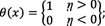
• 6. $f(x, y)=\left\{ {\begin{array}{*{20}l} 1 \hfill & {x_{{0\; \le ~\;x\; \le ~\delta l (length)}} } \hfill \\ {} \hfill & {\left| y \right|\; \le \;~W ~\left( {{\text{width}}} \right)} \hfill \\ 0 \hfill & {{\text{otherwise}}} \hfill \\ \end{array} } \right\}$

• 7. Excitation current in time domain can be expressed as:

  $$J_{s} \left( {x,y,z,t} \right)$$

  where ῃ is the angle of variation in excitation.

Here, we apply excitation through slot dl at some specific angle. Later, shift in the position of slot is provided. Change in radiation pattern or resonant modes is investigated with mathematical equation, simulations and experimentations on RDRA.

$$\frac{{ \mu I \overrightarrow {{{\text{d}}l}} {{e}}^{{ - {j}kr}} }}{4\pi r} = {\vec{A}} ;\;\;{\text{where}}\;A\;{\text{is}}\;{\text{magnetic}}\;{\text{vector}}\;{\text{potential}}$$

(8.1)

$$A = V \cdot \int{E\,{\text{d}}l}$$

$${E} = - j\omega \cdot {\vec{A}}$$

Radiated power

$$\frac{{\left| {E} \right| ^{2} }}{2\eta } = \frac{{\omega^{2} \left| {\vec{A}} \right| ^{2} }}{2\eta }, \quad \quad \sqrt {\frac{\mu }{\epsilon }} = \eta = {\text{impedance}}.$$

(8.2)

$$\underline{{\vec{A}}} = \frac{\mu }{4\pi } \int\limits_{\rm{Volume}}\frac{J\left( {\underline{r}}^{\prime ,\omega }\right){\hbox{$\frac{}{}$}{{e}}}^{{ - jk\left| {\underline{{r}} -\underline{{r}} ^{\prime}} \right|}}}{\left| {\underline{{r}} -\underline{r} ^{\prime}} \right|} d^{3} r^{\prime};\;{{\text{at}\,\,\text{source}}} .$$

(8.3)

We know that radiation pattern can be defined by $E_{\theta } ,\;E_{\phi }$

$$E_{\theta } = - j\omega A_{\theta } \;\;{\text{and}}\;\;{A}_{\theta } = \hat{\theta } \cdot {A}$$

Antenna current density can be expressed as follows:

$$J \cdot ({r^{\prime}} ,\;\omega ) = \mathop \sum \limits_{mnp } {J}_{s} \left[ {mnp,{r^{\prime}} } \right] \quad {{e}}^{{{{j}}\omega \left( {mnp} \right)t}}$$

(8.4)

The magnetic vector potential in terms of J can be written as follows:

$$\begin{aligned} {\underline{A}} = & \frac{\mu }{4\pi }\sum\limits_{mnp} {\int {\frac{{{\underline{J}}_{s} [mnp,\;{\underline{r}^{\prime}} ]{{e}}^{{{{j}}\omega \left( {mnp} \right)\left( {t - \frac{{\left| {{\underline{r}} - {\underline{r}^{\prime}} } \right|}}{c}} \right)}} }}{{\left| {{\underline{r}} - {\underline{r}^{\prime}} } \right|}}} } {\text{d}}s\left( {{\underline{r}^{\prime}} } \right);\quad {\text{d}}s\;{\text{is}}\;{\text{surface}} \\ = & \frac{\mu }{4\pi } \frac{{{{e}}^{{{{j}}kn}} }}{{\left| {{\underline{r}} - {\underline{r}^{\prime}} } \right|}}\sum\limits_{mnp} {\int\limits_{s} {{\underline{J}}_{s} \left[ {mnp,{\underline{r}^{\prime}} } \right] {{e}}^{{{{j}}\omega \left( {mnp} \right){\hat{\underline{r}}} \cdot {\underline{r}^{\prime}} }} {\text{d}}s\left( {{\underline{r}^{\prime}} } \right)} } \\ \end{aligned}$$

(8.5)

$$E_{\theta } , \;E_{\phi } ,\;H_{\phi } = E_{\theta } /\eta ,\;H_{\theta } = - {\raise0.7ex\hbox{${E_{\phi } }$} \!\mathord{\left/ {\vphantom {{E_{\phi } } \eta }}\right.\kern-0pt} \!\lower0.7ex\hbox{$\eta $}}.$$

Radiated power can be given as follows:

$$P_{\text{rad}} = \frac{1}{{2 \eta^{ } }}\left( {\left| {E_{\theta } } \right| ^{2} + \left| {E_{\phi } } \right| ^{2} } \right)$$

(8.6)

$$\left\{ \begin{aligned} \hat{\theta } =\, & \hat{x}\cos \varphi \cos \theta + \hat{y} \sin \varphi \cos \theta - \hat{z}\sin \theta \\ \hat{\phi } = & - \hat{X}\sin \varphi + \hat{Y}\cos \varphi \\ \end{aligned} \right.$$

$$\begin{aligned} E_{\theta } = & \frac{\mu }{{4\pi r^{2} }} \text{Re}\sum\limits_{mnp} {\int\limits_{s} {\left\{ {J_{sx} [mnp,\;{\underline{r}^{\prime}} ]\cos \varphi \cos \theta } \right.} } \\ & \left. { + J_{{sy \left[ {mnp, \;{\underline{r}^{\prime}} } \right]}} \sin \phi \cos \theta - J_{{sz \left[ {mnp,\;{\underline{r}^{\prime}} } \right]}} \sin \theta } \right\} \\ & \quad\exp\left( {{j}\omega \frac{{(mnp)}}{c}} \right)( X^{\prime}\cos \phi \sin \theta + Y^{\prime}\sin \phi \sin \theta + Z^{\prime}\cos \theta ) \text{d}s \left( {\underline{r}^{\prime} } \right)]\;{{e}}^{{{{j}}\omega \left( {mnp} \right)t}} \\ \end{aligned}$$

(8.7)

$$\begin{aligned} E_{\varphi } = & \text{Re} \sum\limits_{{mnp}} {\int {\left\{ { - J_{{sx}} \left( mnp,{\underline{r}^{\prime}} \right)\sin \phi + J_{{sy \left[ {mnp,\;{\underline{r}^{\prime}} } \right]}} \cos \phi } \right\}} } \\ & \quad {e}^{{{j}\frac{{\omega ({mnp})}}{c}}} (X^{\prime}\cos \varphi \sin \theta + Y^{\prime}\sin \phi \sin \theta \\ & \quad \quad \quad \quad\quad\quad + z^{\prime}\cos \theta )\text{d}s\left( {{\underline{r}^{\prime}} } \right){e}^{{{j}\omega \left( {mnp} \right)t}}\text{d}s\left( {{\underline{r}^{\prime}} } \right) \\ \end{aligned}$$

(8.8)

Radiated power P _rad can thus be defined as:

$$P_{x} \left[\hat{r}|~mnp \right] = ~\int\limits_{s} J_{{sx}} \left (mnp,\,{{\underline{r}}^{\prime}}\right) {e}^{{j} \frac{\omega \left( {mnp} \right)\hat{r}\cdot{\underline{r}^{\prime}}}{c}} \text{d}s\left({\underline{r}^{\prime}}\right)$$

(8.9a)

$$P_{y} \left[\hat{r}|~mnp \right] = ~\int\limits_{s} J_{{sy}} (mnp,\,{{\underline{r}}^{\prime}}) {e}^{{j} \frac{\omega \left( {mnp} \right){\underline{\hat{r}}}.{\underline{r}^{\prime}}}{c}} \text{d}s\left({\underline{r}^{\prime}}\right)$$

(8.9b)

$$P_{z} \left[\hat{r}|~mnp \right] = ~\int\limits_{s} J_{{sz}} (mnp,\,{{\underline{r}}^{\prime}}) {e}^{{j} \frac{\omega \left( {mnp} \right){\underline{\hat{r}}}.{\underline{r}^{\prime}}}{c}} \text{d}s\left({\underline{r}^{\prime}}\right)$$

(8.9c)

$$ {\hat{r}( \theta , \phi } ) = \hat{X}\cos \phi \;\sin \theta + \hat{Y}\sin \phi \;\sin \theta + \hat{Z}\cos \theta .$$

Let

$$s = mnp\;{\text{for}}\;{\text{convenience}},\;{\text{then}}$$

$$\begin{aligned} E_{\theta } &= \text{Re} \sum\limits_{s} {\left\{ {P_{x} \left[ {\hat{r}\left| s \right.} \right] \cdot \cos \phi\cos \theta + P_{y } \left[ { \left. {\hat{r}} \right|s} \right]\sin \phi \cos \theta - P_{z} [\left. {\hat{r}} \right|s]\sin \theta \} {{e}}^{j\omega \left( s \right)t} } \right\}} \\ &= \text{Re} \sum\limits_{s} {E_{{s{\theta }}} {{e}}^{j\omega \left( s \right)t} } \\ \end{aligned}$$

(8.10)

$${\text{where}}\quad s = \left( {mnp} \right) = \left[ { \begin{array}{*{20}c} {000} \\ {001} \\ {010} \\ \end{array} } \right] \;{\text{and}}\,\, {\text{so}}\,\, {\text{on }}\,\,{\text{till}}\quad s = \left[ {111} \right]. \;\;{\text{Similarly}}$$

$$E_{\phi } = \text{Re} \sum\limits_{s} {( - P_{x } \left[ {\left. {\hat{r}} \right|s} \right]\sin \varphi + P_{y } \left[ { \left. {\hat{r}} \right|s} \right]\,{\text{cos }}\phi ) {{e}}^{j\omega \left( s \right)t} }$$

(8.11)

Hence, Radiation Pattern of RDRA: Power flux per unit solid angle will describe the pattern. Power radiation pattern can be defined as follows:

$$\begin{aligned} \frac{{\left| {E_{\theta } } \right| ^{2} + \left| {E_{\phi } } \right| ^{2} }}{{2_{\eta } }} = & \frac{1}{2} \left\{ {\left( {\sum\limits_{s} {E_{{s{\theta } }} {{e}}^{j\omega \left( s \right)t} + E_{{s{\phi } }} {{e}}^{j\omega \left( s \right)t} } } \right)} \right\} \times \frac{1}{2}\left\{ {\left( {\sum\limits_{s} {H_{{s{\theta } }} {{e}}^{j\omega \left( s \right)t} + \sum\limits_{s} {H_{{s{\phi } }} {{e}}^{j\omega \left( s \right)t} } } } \right)} \right\} \\ = & \frac{1}{4} \left( {\sum\limits_{s} {E_{s} \times H_{m}^{*} {{e}}^{{j\left( { \omega_{s} - \omega_{m} } \right)t }} } + \sum\limits_{s} {E_{s}^{*} \times H_{m} {{e}}^{{j\left( { \omega_{m} - \omega_{s} } \right)t }} } } \right) \\ = & \frac{1}{4} \sum\limits_{s} {\left[ {E_{s\theta } \times H_{s\oslash }^{*} + E_{s\oslash }^{*} \times H_{s\theta }^{ } } \right]} \\ = & \frac{1}{2} \text{Re} \sum\limits_{s} {\left( { E_{s\theta } \times H_{s\oslash }^{*} } \right)} \\ = & \frac{1}{2} \left( { E_{{s{\theta } }} \hat{\theta } + E_{\oslash } {\hat{\oslash}} } \right) \times \left( {\frac{{E_{s\theta }^{*} }}{\eta }\hat{\varphi} - \frac{{E_{s\oslash }^{ } }}{\eta }\hat{\theta }} \right) \\ = & \sum\limits_{s} {\frac{{\left| {E_{{s{\theta } }} } \right|^2}}{2\eta }} \hat{r} + \frac{{\left| {E_{{s{\oslash } }} } \right|^2}}{2\eta } \hat{r} \\ \end{aligned}$$

(8.12)

Poynting vector

$$\begin{aligned} {S} \cdot \hat{r} &= \frac{1}{2\eta } \sum {\left[ {\omega (s)^{2} \left| {P_{x} (\hat{r}} \right|s)\cos \phi \cos \theta + P_{y} \left( {\hat{r}\left| s \right.} \right)\sin \varphi \cos \theta - \left. {P_{z} \left( {\hat{r}\left| s \right.} \right)\sin \theta } \right|^{2} } \right.} \hfill \\ & \left. {\quad + \,\,\omega (s)^{2} \left| {P_{x} (\hat{r}} \right|s)\sin \varphi - \left. {P_{y} \left( {\hat{r}\left| s \right.} \right)\cos \varphi } \right|^{2} } \right] \hfill \\ \end{aligned}$$

(8.13)

Radiated power per unit solid angle or Poynting vector

$$\ \begin{aligned} {S} \cdot \hat{r} \left( {r,\theta, \phi } \right) = & \frac{1}{{2\eta }}\sum\limits_{{{mnp}}} {\omega (mnp)^{2} } \left\{ {\left| {P_{x} (\theta ,\phi } \right|mnp{\text{)}}\;\cos \phi \;\cos \theta } \right. \\ & + P_{y} \left( {\theta ,\phi \left| {mnp} \right.} \right)\;\sin \phi \;\cos \theta - P_{z} \left( {\theta ,\phi \left| {mnp} \right.} \right)\;\sin \theta \left| {^{2} } \right. \\ & \left. { +\,\left| {P_{x} (\theta ,\phi } \right|mnp)\;\sin \phi \pm P_{y} \left( {\theta ,\phi \left| {mnp} \right.} \right)\;\cos \phi \left| {^{2} } \right.} \right\} \\ \end{aligned}$$

(8.14)

8.3 Radiation Pattern Based on Angle ${\varvec{(\oslash}}_{\mathbf{0}} ,{\varvec{{\phi}_{\mathbf{0}}}} \varvec{)}$ Variation in xy Plane

$${\text{Let }}\tilde{D}_{{\left( {mnp} \right)}} = \frac{\pi p}{d} \frac{{\hat{D}_{{ {mnp} }} }}{{h_{mn}^{2} }}\;{{e}}^{{j\psi {mnp} }}$$

$$\tilde{C}_{{ {mnp} }} = \frac{\epsilon }{{h_{mn}^{2} }} {e}^{{j\left( {\phi \left( {mnp} \right) - {\raise0.7ex\hbox{$\pi $} \!\mathord{\left/ {\vphantom {\pi 2}}\right.\kern-0pt} \!\lower0.7ex\hbox{$2$}}} \right)}} \hat{C}_{{ {mnp}}}$$

$$H_{ \bot } = \left[ {\mathop \sum \limits_{mnp}^{ } \text{Re} \;\{ \tilde{D}_{{ {mnp} }} {{e}}^{{j\omega ({mnp})t}} \} \nabla_{ \bot } \tilde{u}_{mnp} \left( {x,y,z} \right)} \right]\mathop \sum \limits_{mnp}^{ } \text{Re} \;\left\{ {\tilde{C}_{{ {mnp} }} {{e}}^{{j\omega \left( {mnp} \right)t}} } \right\} \nabla_{ \bot } \tilde{u}_{mnp} \left( {x,y,z} \right)$$

(8.15)

Probe orientation

$$\hat{n}\left( { \theta_{0} ,\; \phi_{0} } \right) = \hat{x}\;\cos \phi_{0} \;\sin \theta_{0} + \hat{y} \;\sin \phi_{0} \;\sin \theta_{0} + \hat{z}\;\cos \phi_{0}$$

$$\hat{n} \times {H} = J_{s}$$

$$h_{m n}^{2} = \gamma^{2} + k^{2} = n_{x} \hat{x} + n_{y} \hat{y} + n_{z} \hat{z}$$

$$\gamma = \pm \frac{jp\pi }{d};\;{\text{for}}\;{\text{all}}\;{\text{wave}}\;{\text{guide}}\;{\text{and}}$$

$${\text{let}}\quad\upgamma = \frac{\text{d}}{\partial z} , \quad j\omega = \frac{\text{d}}{{{\text{d}}t}} ;\;{\text{for all cavity resonator }}$$

$$\delta l\;\cos \theta_{0} = \delta ;\;{\text{Probe length}}$$

Matrix-based computations are as follows:

$$\left\{ {\begin{array}{*{20}c} {E_{z} } & {E_{ \bot } } \\ {H_{z} } & {H_{ \bot } } \\ \end{array} } \right\}$$

$$\begin{aligned} H_{x} & = J_{sy} \\ H_{y} & = - J_{s x} \\ H_{ \bot } & = H_{x} \hat{x} + H_{y} \hat{y} \\ \end{aligned}$$

$$E_{z} = \sum\limits_{mnp} {\text{Re} \left[ {{C}_{{ {mnp} }} u_{{ {mnp} }} \left( {x,y,z} \right)} \right] {\exp}(j\omega_{{ {mnp} }} t)}$$

(8.16)

$$H_{ \bot } = \frac{ - \gamma }{{h^{2}_{mnp} }}\quad \nabla_{ \bot } H_{z} + \frac{j\omega \epsilon }{{h^{2}_{mnp} }} \nabla_{ \bot } E_{z} \times \hat{z}$$

(8.17)

$$H_{z} = u_{mn} \left( {x,y} \right)\,{\exp}\left( {\frac{j\pi pz}{d}} \right)$$

(8.18)

$$H_{z} = u_{mn} \left( {x,y} \right) {C} ({mnp}) {{e}}^{{{j}}\left( {\omega \left( {m n p} \right)t} - \frac{jp\pi z}{d}\right)}$$

$$H_{z} = {\text{Re}} \left\{ {{C}_{{ {mnp} }} u_{mn} \left( {x,y} \right) {{e}}^{{ \pm {{j}}\left( {\omega \left( {m n p} \right)t - \frac{jp\pi z}{d}} \right)}} } \right\}$$

$$\begin{aligned} H_{z} = & \text{Re}\left\{ {C_{1} \left( {mnp} \right)u_{{mn}} \left( {x,y} \right){e}^{{j(\omega \left( {mnp} \right)t - \frac{{jp\pi z}}{d})}} } \right\} \\ & + \text{Re} \left\{ {C_{2} \left( {mnp} \right)u_{{mn}} \left( {x,y} \right){e}^{{ - j(\omega \left( {mnp} \right)t + \frac{{jp\pi z}}{d})}}} \right\}\\ \end{aligned}$$

(8.19)

$$H_{ \bot } = \left[{\frac{1}{{h^{2}_{{mn_{ } }} }}\frac{\text{d}}{{\text{d}z }} \nabla_{\bot } H_{z} \left({ x,y,z,t} \right)} \right] + \left[{\frac{\epsilon }{{h_{mn}^{2} }}\frac{\partial }{\partial t} \nabla_{\bot} E_{z} ( x,y,z,t)} \right]$$

(8.20)

Hence

$$E_{z} \left( {x,y z,t} \right) = \sum\limits_{mnp} {C_{{{mnp}}} u_{{ {mnp} }} \left( {x,y,z} \right)\cos \left( {\omega ({mnp})t + \varphi ({mnp})} \right)}$$

(8.21a)

$$H_{z} \left( {x,y z,t} \right) = \sum\limits_{mnp} {D_{{{mnp}}} u_{{{mnp}}} \left( {x,y,z} \right)\;{ \cos}\left( {\omega \left( {mnp} \right)t + \psi \left( {mnp} \right)} \right)}$$

(8.21b)

8.4 Replacing Probe with Slot of Finite Dimensions (Ls, Ws) at an Angle ${{{\varvec{(}}{\varvec{\theta}}_{\mathbf{0}}}} ,{{\varvec{\phi}_{\mathbf{0}}}} )$

We replace excitation probe to slot u _mnp and v _mnp by $\tilde{u}_{mnp}$ and $\tilde{v}_{mnp}$

$$\tilde{u}_{mnp} \left( {x,y,z} \right) = \frac{{2\sqrt[ ]{2}}}{{\sqrt {abd} }} \;\sin \left( {\frac{m\pi x}{a}} \right)\;{ \sin }\left( {\frac{n\pi y}{b}} \right)\;{ \sin }\left( {\frac{\rho \pi z}{d}} \right)$$

(8.22a)

$$\tilde{v}_{mnp} \left( {x,y,z} \right) = \frac{{2\sqrt[ ]{2}}}{{\sqrt {abd} }}\;\cos\left( {\frac{m\pi x}{a}} \right)\;{\text{cos}}\left( {\frac{n\pi y}{b}} \right)\;{\text{cos}}\left( {\frac{\rho \pi z}{d}} \right)$$

(8.22b)

$$J_{s} \left( {x,y,\delta } \right) = \frac{{I[_{mnp} ] {{e}}^{{\eta '\omega \left( {mnp} \right)t}} }}{\omega } ; \;{\text{where}}\; \eta^{\prime}\; {\text{is}}\;{\text{an}}\;{\text{angle }}$$

$$\begin{aligned} \left. {{H}_{ \bot } } \right| _{{z_{ = \delta } }} = & \sum\limits_{mnp} {\text{Re} \;\left\{ {\tilde{D}_{{ {mnp} }} {{e}}^{{{{j}}\omega \left( {mnp} \right)t}} } \right\}} \nabla_{ \bot } \tilde{v}_{mnp} \left( {x,y,z} \right) \\ & \quad - \sum\limits_{mnp} {\text{Re} \;\left\{ {\tilde{C}_{{{mnp}}} {{e}}^{{{{j}}\omega \left( {mnp} \right)t}} } \right\}\nabla_{ \bot } \tilde{u}_{mnp} \left( {x,y,z} \right)} \\ \end{aligned}$$

(8.23)

$$\hat{n} \times {H}$$

$E_{x} , E_{y} , H_{x} ,\;H_{y}$ are the fields in terms of surface current density due to applied probe current at an angle η′; $J _{sx } , J _{sy}$ can be expressed as current density using Fourier coefficients; ${C}_{{{mnp} }} \;{\text{and}}\;D_{{ {mnp} }}$ $H_{y} H_{x}$ fields can be computed from $E_{x} E_{y} \;\text{fields}$; propagation terms $h_{mn}^{2} = \gamma^{2} + k^{2}$

$${H}_{ \bot } = {\frac{{I_{{{mnp} }} }}{{\omega_{{\left( {\text{width}} \right)}} }} {{e}}^{{j\eta \left( {mnp} \right)}} \{ \hat{x} - \left( {\sin (\phi_{0} } \right)\;\cos \left( {\phi_{0} } \right)\hat{y})\} g (x,y)} $$

$$H_{ \bot } = \sum\limits_{mnp} {\text{Re} \{ \tilde{D}_{{{mnp}}} {{e}}^{{j\omega \left( {mnp} \right)t}} \frac{{2\sqrt[ ]{2}}}{{\sqrt {abd} }} \nabla_{ \bot } \left\{ {\cos \left( {\frac{m\pi x}{a}} \right)\cos \left( {\frac{n\pi y}{b}} \right)} \right\}} .$$

(8.24)

$$\begin{aligned} {H}_{ \bot } \left| \right._{{z_{ = 0} }} =\,& H_{X} \left( {x,y,0} \right)\hat{x} + H_{Y} \left( {x,y,0} \right)\hat{y} \\ =\,& \left\{ { J_{sy} \left( {x,y,t} \right) - J_{sx} \left( {x,y,t} \right)} \right\} \\ \end{aligned}$$

$$J_{sy} \left( {x,y,t} \right) = \sum {\text{Re} \left\{ {\tilde{D}_{{{mnp}}} {{e}}^{{j\omega \left( {mnp} \right)t}} } \right\} \left( {\frac{m\pi }{a}} \right)\frac{{2\sqrt[ ]{2}}}{{\sqrt {abd} }}\;\sin \left( {\frac{m\pi x}{a}} \right)\;\cos \left( {\frac{n\pi y}{b}} \right)}$$

$$\begin{aligned} & \int\limits_{0}^{a} {\int\limits_{0}^{b} {J_{sy} \left( {x,y,t} \right)} } \frac{2}{{\sqrt {ab} }}\sin \left( {\frac{m\pi x}{a}} \right)\cos \left( {\frac{n\pi y}{b}} \right) {\text{d}}x{\text{d}}y \\ & \quad = \text{Re} \left\{ {\tilde{D}_{{ {mnp} }} {{e}}^{{j\omega \left( {mnp} \right)t}} } \right\} \left( {\frac{m\pi }{a}} \right)\sqrt {\frac{2}{d}{ \sin }\left( {\frac{m\pi x}{a}} \right)} \\ \end{aligned}$$

Hence,

$$J_{{sy}} \left( {x,y,t} \right) = \text{Re} \left\{ {f_{y} \left( {x,y} \right){{e}}^{{{{j}}\omega \left( {mnp} \right)t}} } \right\} = \int\limits_{0}^{a} {\int\limits_{0}^{b} {f_{y} \left( {x,y} \right)} } \frac{2}{{\sqrt {ab} }}\sqrt {\frac{2}{d}} ,\left( {\frac{{m\pi }}{a}} \right)\tilde{D}_{{{mnp}}} \sin \left( {\frac{{m\pi x}}{a}} \right)\cos \left( {\frac{{n\pi y}}{b}} \right){\text{d}}x{\text{d}}y$$

(8.25)

Now

$$\tilde{D}_{{{mnp} }} = \sqrt {\frac{2}{d}} \frac{a}{{m\pi }}\int\limits_{0}^{a} {\int\limits_{0}^{b} {f_{y} \left( {x,y} \right)} } \frac{2}{{\sqrt {ab} }}\sin \left( {\frac{{m\pi x}}{a}} \right)\cos \left( {\frac{{n\pi y}}{b}} \right){\text{d}}x{\text{d}}y$$

(8.26)

$$H_{y} = - J_{sx}$$

$$- J_{sx} \left( {x,y,t} \right) = {H}_{y} \left| \right._{{z_{ = 0} }} = \sum\limits_{mnp} {\text{Re} \;\left\{ {\tilde{D}_{{ {mnp} }} {{e}}^{{j\omega \left( {mnp} \right)t}} } \right\}\left( {{-}\frac{n\pi }{b}} \right)\frac{{2\sqrt[ ]{2}}}{{\sqrt {abd} }}\;\cos \left( {\frac{m\pi x}{a}} \right)\;\cos \left( {\frac{n\pi y}{b}} \right)}$$

(8.27)

$$J_{sx} \left( {x,y,t} \right) = \text{Re} \left\{ { f_{x} \left( {x,y} \right){{e}}^{{ + j\omega \left( {mnp} \right)t}} } \right\}$$

$$\tilde{D}_{{{mnp}}} = \frac{2}{ab} \sqrt[ ]{\frac{2}{d}} \frac{b}{n\pi } \mathop \int \limits_{0}^{a} \mathop \int \limits_{0}^{b} f_{x} \left( {x,y} \right)\;\cos \left( {\frac{m\pi x}{a}} \right)\;\cos \left( {\frac{n\pi y}{b}} \right)\;{\text{d}}x {\text{d}}y$$

$$J_{sx} \left( {x,y,t} \right) = \sum\limits_{mnp} {{\text{Re}}\{ f_{x} \{ x,y|mnp\} {{e}}^{{j\omega \left( {mnp} \right)t}} }$$

(8.28)

$${\text{Similarly}},\;{\text{compute}}\;\tilde{D}_{{ {mnp} }}{:}$$

$$J_{sy} \left( {x,y,t} \right) = \sum\limits_{mnp} {{\text{Re}}\{ f_{y} \{ x,y|mnp \} {{e}}^{{j\omega \left( {mnp} \right)t}} }$$

(8.29)

8.5 HFSS Computed Radiation Pattern with Shifted ${{(\varvec{\theta}_{\varvec{i}} ,{\varvec{\phi}_{\varvec{i}}}}} )$ Slot Positions

Angular excitation at 45° and 30° left side.

Results of angular excitation on radiation pattern have been evaluated on HFSS and shown in Fig. 8.5.

Angular shifts in excitation at 45° and 30° right side and radiation pattern are shown in Fig. 8.7 and summarized are placed in Table 8.1.

Table 8.1 Summarized results

Results of Radiation pattern when angular excitation is given to the right side have been shown in Fig. 8.7.

Table 8.1 described results of antenna parameters in tabular form. It has been observed that angular variation in excitation has direct impact on the radiation pattern as well as number of modes generated. This has been verified by the plots given above. We have taken measurements of radiation pattern on varying slot of feed at 30° and 45° to left and right from its original position. These plots have been verified at two different frequencies. This completes the solution.

8.6 Experimentations

Figures 8.8, 8.9, 8.10, 8.11, 8.12, 8.13, 8.14, 8.15 and 8.16 present the experimental results of RDRA. Their significance is placed below each figure. The RDRA made from acrylic glass sheets having dimensions of 9, 6 and 3 cm. The silicon oil having $\varepsilon = 2.2$ was used as RDRA dielectric material. The resonant frequency of RDRA was measured to 4.55 GHz. The measurements were taken at various angular positions of the slot. Aperture-coupled feed RDRA is shown in Fig. 8.1. The feed position was shifted to investigate RDRA S ₁₁ using VNA 40 GHz. The results are shown in Figs. 8.2, 8.3, 8.4 and 8.5.

Fig. 8.8

RDRA under measurements with VNA

Fig. 8.9

−28.23 dB measured S ₁₁ of RDRA at 4.63 GHz

Fig. 8.10

S ₁₁ RDRA with shifted slot resonant frequency 3.67

Fig. 8.11

Smith chart showing proper Z ₁₁ of RDRA

Fig. 8.12

S ₁₁ at shifted slot frequency 3.57 GHz

Fig. 8.13

Measurements of RDRA with aspect ratio changed

Fig. 8.14

RDRA aspect ratio changed

Fig. 8.15

Shifted frequency observed (3.60 GHz)

Fig. 8.16

Aperture-coupled feed showing slot

The results obtained with VNA have clearly shown shift in resonant frequency due to feed orientation. It indicated that resonant modes are changing based on the slot orientation. Hence, it is clearly evident that radiation pattern can be steered with slot position in RDRA . If these results can be placed in look up table, then microcontroller-based orientation can result into automated antenna. This automated antenna can be very useful for military applications. These cross slot can be  arranged  in such a manner  that circular polarization becomes possible in RDRA. Also by varying lengths of cross slots,  left hand or right hand polarization can be achieved. The circular  ploarization makes the signal robust and help to reduce  electromagnetic  polution.