Quantifying and Propagating Uncertainty in Automated Linked Data Integration

Abstract

The Web of Data consists of numerous Linked Data (LD) sources from many largely independent publishers, giving rise to the need for data integration at scale. To address data integration at scale, automation can provide candidate integrations that underpin a pay-as-you-go approach. However, automated approaches need: (i) to operate across several data integration steps; (ii) to build on diverse sources of evidence; and (iii) to contend with uncertainty. This paper describes the construction of probabilistic models that yield degrees of belief both on the equivalence of real-world concepts, and on the ability of mapping expressions to return correct results. The paper shows how such models can underpin a Bayesian approach to assimilating different forms of evidence: syntactic (in the form of similarity scores derived by string-based matchers), semantic (in the form of semantic annotations stemming from LD vocabularies), and internal in the form of fitness values for candidate mappings. The paper presents an empirical evaluation of the methodology described with respect to equivalence and correctness judgements made by human experts. Experimental evaluation confirms that the proposed Bayesian methodology is suitable as a generic, principled approach for quantifying and assimilating different pieces of evidence throughout the various phases of an automated data integration process.

1 Introduction

There has been a general trend towards generating large volumes of data, especially with the explosion of social media and other sensory data from smart devices. The Web is no exception to the accelerating and unprecedented rate at which digital data is being generated. Because of this explosion, data is now made available with different characteristics: with different degrees of structure (e.g., structured or unstructured), often semantically annotated (e.g., Linked Data (LD)), typically stored in various distributed data sources¹, often designed independently using different data models, and maintained autonomously by different actors. This makes it imperative to integrate data from various sources with the aim of providing transparent querying facilities to end-users [19]. However, this integration task poses several challenges due to the different types of heterogeneities that are exhibited by the underlying sources [10, 12]. For instance, in the case of the Web of Data (WoD), LD sources do not necessarily adhere to any specific, uniform structure and are, thus, considered to be schema-less [5]. This can lead to a great diversity of publication processes, and inevitably means that resources from the same domain may be described in different ways, using different terminologies.

The challenging problem of resolving the different kinds of heterogeneities that data sources exhibit with the aim of providing a single, transparent interface for accessing the data is known as data integration [10, 12]. A traditional data integration system [19] builds on a mediator-based architecture where a virtual schema is designed that captures the integration requirements and is presented to the user for querying. In this approach, the integration schema is seen as a logical schema since the data still resides in the underlying data sources (as opposed to being materialized, as is typically the case for data warehouses). Typically, for the underlying sources to interoperate, two basic capabilities are required: (i) matching, i.e., the ability to quantify the degree of similarity between the source schemas and the integration schema (often by considering their terminologies, and, if available, samples of instance data), the result of which is a set of semantic correspondences (a.k.a. matches); and (ii) mapping generation, i.e., the ability to use the set of semantic correspondences in order to derive a set of executable expressions (a.k.a. mappings) that, when evaluated, translate source instance data into instance data that conforms to the integration schema.

Dataspaces are data integration systems that build on a pay-as-you-go approach for incremental and gradual improvement of automatically derived speculative integrations [20, 30]. In this approach, the manual effort required to set up a traditional data integration system is replaced with automatic techniques that aim to generate a sufficiently useful initial integration with minimum human effort [11, 14]. Over time, as the system is continuously queried, users are stimulated to provide feedback (e.g., on query results) that, once assimilated, lead to a gradual improvement in the quality of the integration [2]. More specifically, with a view to providing best-effort querying capabilities, dataspaces are envisioned to have a life-cycle (depicted in Fig. 1) comprising the following phases: (i) bootstrapping, where algorithmic techniques are used to automatically derive an initial integration by postulating the required semantic correspondences and using them to derive mappings between the source schemas and the integration schema²; (ii) usage, where best-effort querying services are provided to answer user requests over the speculative integration, and explicit or implicit feedback [24] is collected to inform the incremental improvement of the integration; and finally (iii) improvement, where the feedback that has been collected during usage is assimilated in order to improve the initial integration, e.g., by filtering erroneously-derived semantic correspondences and regenerating the mappings previously derived from them.

Fig. 1.

Dataspace life-cycle phases.

Because dataspaces depend on automation, and because automation can only generate inherently uncertain outcomes, it is imperative to quantify and propagate uncertainty throughout the dataspace life-cycle [18, 31]. Broadly speaking, it is not obvious how the inherent uncertainty arising during the various phases of a dataspace system can be quantified and then reasoned with in a principled manner. Motivated by this challenge, and taking into account the different types of uncertainty that must be quantified and propagated across the phases of the dataspace life-cycle, this paper contributes a methodology for quantifying uncertainty (founded on the construction of empirical probabilistic models based on kernel estimators) and for reasoning with different kinds of evidence that emerge during the boostrapping phase of a dataspace system using Bayesian techniques for assimilating: (a) syntactic evidence, in the form of similarity scores generated by string-based matchers, (b) semantic evidence, in the form of semantic annotations such as subclass-of and equivalent relations that have been asserted in, or inferred from, LD ontologies, and (c) internal evidence, in the form of mapping fitness values, produced during mapping generation.

1.1 Motivating Example: Uncertainty in Dataspaces

Our motivating example comes from the music domain. We assume the inferred schemas for the Jamendo LD source³, denoted by $s_1$, and the Magnatune LD source⁴, denoted by $s_2$, depicted in simplified ER notation in Fig. 2 (a) and (b), respectively. The goal is integrate these to give rise to an integrated schema, denoted by $s_{int}$.

Fig. 2.

Inferred schemas from LD sources.

For the identification of these candidate semantic matches, several approaches have been proposed especially by the literatures on schema matching [27] in the database area, and on ontology alignment [32] in the knowledge representation area. Figure 3 shows a subset of semantic correspondences (i.e., matches) that might have been discovered across our example schemas using string-based matching techniques (e.g., n-gram).

Fig. 3.

Example schema matching results.

Figure 4 exemplifies different kinds of semantic evidence regarding our example schemas. In this figure, solid arrows denote annotations (e.g., rdfs:subClassOf) either internal, pointing to constructs in the same LD vocabulary, or external, pointing to constructs in some other LD vocabulary; dashed arrows denote equivalence annotations that define entities; and dotted lines show examples of one-to-one semantic correspondences where confidence is measured as a d.o.b. As this example shows, semantic relationships may exist in addition to syntactic ones, e.g., mo:MusicGroup is also subsumed by foaf:Group and not simply named in a syntactically similar way to the latter. Section 3.2 presents a methodology for quantifying semantic evidence that is founded on the construction of probabilistic models that can be used to inform a Bayesian approach for making judgements on the equivalence of constructs.

Fig. 4.

Different kinds of semantic evidence.

Table 1 shows examples of such internal evidence viz., where the fitness values and corresponding mapping correctness score (as explained in Sect. 2) are assumed to have been returned by the mapping generation process. Some examples of mapping queries are provided in Table 2.

Table 1. Example of internal evidence from the mapping generation phase.

1.2 Summary of Contributions

This paper describes a probabilistic approach for combining different types of evidence so as to annotate integration constructs with d.o.b.s on semantic equivalence and on mapping quality. This paper contributes the following: (a) a methodology that uses kernel density estimation for deriving likelihoods from similarity scores computed by string-based matchers; (b) a methodology for deriving likelihoods from semantic relations (e.g., rdfs: subClassOf, owl:equivalentClass) that are retrieved by dereferencing URIs in LD ontologies; (c) a methodology for aggregating evidence of conceptual equivalence of constructs from both string-based matchers and semantic annotations; (d) a methodology for deriving likelihoods from mapping fitness values and mapping correctness scores using bivariate kernel density estimation; and (e) an empirical evaluation of our approach grounded on the judgements of experts in response to the same kinds of evidence. Note that, in this paper, the experiments only use LD datasets.

The remainder of the paper is structured as follows. Section 2 presents an overview of the developed solution. Section 3 describes the contributed methodologies. The application of bayesian updating, as a technique for the incremental assimilation of data integration evidence, is introduced in Sect. 4. Section 5 presents an empirical evaluation of the methodology complemented by a discussion of results. Section 6 reviews related work, and Sect. 7 concludes.

2 Overview of Solution

The main focus of this paper is on the bootstrapping phase of a data integration system. More specifically, the techniques discussed in this section focus on opportunities for the quantification and assimilation of uncertainty using a Bayesian approach to assimilate different forms of evidence. Figure 5 stands in contrast with Fig. 1 and indicates the different types of evidence that inform different bootstrapping stages in our approach. Our techniques have been implemented as extensions to the DSToolkit [13] dataspace management system, which brings together a variety of algorithmic techniques providing support for the dataspace life-cycle.

Deriving d.o.b.s on Matches. Assuming that declared (or else inferred) conceptual descriptions (e.g., schemas) for the sources and target integrated artefact are available, the basic notion underpinning the bootstrapping process is that of semantic correspondences. Given a conceptual description of a source and a target LD dataset, denoted by S and T, respectively, a semantic correspondence is a triple $\langle c_S, c_T, P(c_S \equiv c_T | E) \rangle$, where $c_S \in S$ and $c_T \in T$ are constructs (e.g., classes, or entity types) from (the schema of) the datasets, and $P(c_S \equiv c_T | E)$ is the conditional probability representing the d.o.b. in the equivalence ($\equiv$) of the constructs given the pieces of evidence ${(e_1,\ldots ,e_n)} \in E$. Such semantic correspondences, therefore, quantify (as d.o.b.s) the uncertainty resulting from automated matching techniques that yield syntactic evidence in the form of similarity scores but also taking into account, when available, semantic annotations from ontologies (as exemplified in Fig. 4).

Deriving d.o.b.s on Mappings. Given a set of semantic correspondences, the mapping generation process derives a set of mappings M using (in the case of DSToolkit) an evolutionary search strategy that assigns a fitness value to each mapping in the solution set. A mapping $m \in M$ denotes that one or more schema constructs from S that can be used to populate one or more constructs from T. The two sets of schema constructs that are related in this way by a mapping are henceforth referred to as entity sets and notated as $\langle ES^S,ES^T\rangle$, where $ES^S \in S$ and $ES^T \in T$.

Fig. 5.

Uncertainty propagation and evidence assimilation.

Table 2. Example generated mappings.

As a result of the search technique used in the mapping generation process, a mapping fitness value y is a measure of the strength of the internal evidence that a set of schema constructs in a source entity set $ES^S$ is semantically related to a set of schema constructs in the target entity set $ES^T$. In this context, $P(m \mid f(m)=y)$ is the conditional probability representing the d.o.b. that an attribute value in a tuple returned by the mapping m is likely to be correct, given that the fitness value of m, is y i.e., $f(m)=y$. Such probabilities, therefore, quantify (as d.o.b.s) the uncertainty resulting from the automated mapping generation technique used, i.e., one that yields mapping fitness values. Table 2 shows some mappings generated between a target schema, denoted by $s_{int}$ and source schemas, denoted by $s_1$, and $s_2$, resp., along with their associated fitness value scores.

Types of Evidence. As indicated above, our approach makes use of three distinct types of evidence: (a) syntactic evidence, in the form of strings that are local-names of resource URIs; (b) semantic evidence, such as structural relations between entities, either internal to a vocabulary or across different LD vocabularies (e.g., relationships such as subclass of and equivalence); and (c) internal evidence, in the form of fitness values computed during mapping generation. Table 3 briefly describes the types of evidence used in this paper and introduces the abbreviations by which we shall refer to them. In particular, if TE is the set of all semantic annotations, its subsets EE and NE comprise the assertions that can be construed as direct evidence of equivalence and non-equivalence, respectively.

Table 3. Types of evidence.

Collecting Evidence. To collect syntactic evidence (represented by the set LE), given two sources, our approach extracts local names from the URIs of every pair of constructs $\langle c_s, c_t \rangle$ and then derives their pairwise string-based degree of similarity. Two string-based metrics are used in our experiments, viz., edit-distance (denoted by ed) and n-gram (denoted by ng) [32]. Section 3.1 explains in detail how probability distributions can be constructed for each matcher. To collect semantic evidence, our approach dereferences URIs to obtain access to annotations from the vocabularies that define the resource. For example, the subsumption relation $c_S \sqsubseteq c_T$ is taken as semantic evidence. Section 3.2 explains in detail how to construct probability distributions for each kind of semantic evidence published in RDFS/OWL vocabularies. To collect evidence on mapping generation, we extract from the set of mappings generated by a mapping generation algorithm their fitness value, and, therefore, we assume that the search procedure underpinning the algorithm aims to maximize an objective function founded on such fitness values [8]. Section 3.3 explains in detail how to construct probability distributions for mapping fitness values. Later in our methodology, the probability distributions thus constructed are used to denote the likelihood of evidence term in Bayes’s formula.

We use a Bayesian approach to evidence assimilation, i.e., given a degree of uncertainty expressed as a d.o.b., once new evidence is observed, we use Bayes’s formula to update that d.o.b. (referred to as the prior) into a new d.o.b. (referred to as the posterior) that reflects the new evidence. Applying Bayes’s formula in this way requires us to quantify the uncertainty of the evidence (referred to as the likelihood). This means that in order to assimilate different kinds of evidence, preliminary work is needed to enable the computation of the likelihoods in applications of Bayes’s formula, i.e., the otherwise unknown term required for the calculation of a posterior d.o.b. from a prior d.o.b. This requirement holds for the equivalence of constructs, as captured by the posterior $P(c_S \equiv c_T|E)$ when the evidence is syntactic (as described in Sect. 3.1) and when the evidence is semantic (as described in Sect. 3.2). Similarly, preliminary work is needed for deriving a d.o.b. on mapping correctness, as captured by the posterior $P(m \mid f(m)=y)$, where $f(m)=y$ is internal evidence from mapping generation in which we relate the notion of mapping correctness to the fraction of correct attribute values in a mapping extent (as described in Sect. 3.3).

The idea behind Bayesian updating [34] is that once the posterior (e.g., $P(c_S \equiv c_T | E)$) is computed for some evidence $e_1 \in E$, a new piece of evidence $e_2 \in E$ allows us to compute the impact of $e_2$ (i.e., measure how the d.o.b. is changed in light of $e_2$) by taking the previously computed posterior as the new prior.

3 Constructing Likelihoods for Evidence

We now provide a detailed account of a principled methodology for constructing probability distributions from relevant evidence with a view towards enabling a Bayesian approach to quantifying and propagating uncertainty across the dataspace life-cycle.

3.1 Deriving Likelihoods for Similarity Scores

We call syntactic evidence the likelihoods derived from similarity scores produced by string-based matchers. We study the behaviour of each matcher (in our case ed and ng) used to derive similarity scores.

To derive probability density functions (PDFs) for syntactic evidence, we proceeded as follows:

• 1. From the datasets made available by the Ontology Alignment Evaluation Initiative (OAEI)⁵, we observed the available ground truth on whether a pair of local-names, denoted by $(n, n')$, aligns.

• 2. We assumed the existence of a continuous random variable, X, in the bounded domain [0, 1], for the similarity scores returned by each matcher $\mu$, where $\mu \in \{{\textsf {ed}}, {\textsf {ng}}\}$. Our objective was to model the behaviour of each matcher in terms of a PDF f(x) over the similarity scores it returns, which we refer to as observations in what follows.

• 3. To empirically approximate f(x) for each matcher, we proceeded as follows:

  • (a) We ran each matcher $\mu$ independently over the set of all local-name pairs $(n,n')$ obtained from (1).

  • (b) For each pair of local-names, we observed the independent similarity scores returned by the matcher when $(n, n')$ agrees with the ground truth. These are the set of observations ($x_1,\ldots ,x_i$) from which we estimate f(x) for the equivalent case.

• 4. The observations $x_1,\ldots ,x_i$ obtained were used as inputs to the non-parametric technique known as kernel density estimation (KDE) (using a Gaussian kernel⁶) [4] whose output is an approximation $\hat{f}(x)$ for both ed and ng and for both the equivalent and non-equivalent cases.

We interpret the outcome of applying such a PDF to syntactic evidence as the likelihood of that evidence. More formally, and as an example, $PDF\,{{\underset{ed}{\equiv }}}\,(\mathsf {ed}(n, n'))\,=\,P(\mathsf {ed}(n, n') | c_S \equiv c_T)$, i.e., given a pair of local-names $(n, n')$ the PDF for the ed matcher in the equivalent case $PDF\,{{\underset{ed}{\equiv }}}$ yields the likelihood that the similarity score $\mathsf {ed}(n, n')$ expresses the equivalence of the pair of concepts $(c_S,c_T)$ that $(n, n')$, resp., denote. Correspondingly, for the non-equivalent case, and for ng in both the equivalent and non-equivalent cases.

The PDFs derived by the steps described above are shown in Fig. 6(a) and (b) for ed and in Fig. 6(c) and (d) for ng. The same procedure can be used to study the behaviour of any matcher that returns similarity scores in the interval [0, 1]. Note that the PDFs obtained by the method above are derive-once, apply-many constructs. Assuming that the samples used in the estimation of the PDFs remain representative, and given that the behaviour of matchers ed and ng is fixed and deterministic, the PDFs need not be recomputed.

3.2 Deriving Likelihoods for Semantic Evidence

We call semantic evidence the likelihoods derived from semantic annotations obtained from the WoD. We first retrieved the semantic annotations summarised in Table 3. The set TE is the set of all such evidence, $TE = SU \cup SB \cup SA \cup EC \cup EM \cup DF \cup DW$. We formed the subsets $EE \subset TE = SA \cup EC \cup EM$ and $NE \subset TE = DF \cup DW$ comprising assertions that can be construed as direct evidence of equivalence and non-equivalence, respectively.

Fig. 6.

Illustration of probability distributions for each matcher over [0, 1].

To derive a PDF for semantic evidence, we proceeded as follows:

• 1. We assumed the existence of a Boolean random variable, for each type of semantic evidence in Table 3, with domain $\{true, false\}$.

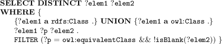
• 2. Using the vocabularies available in the Linked Open Vocabularies (LOV)⁷ collection, we collected and counted pairs of classes and properties that share direct or indirect assertions of equivalence or non-equivalence for all the assertions in TE and NE using SPARQL queries. For example, with respect to equivalence based on OWL and RDFS class annotations:

  

• 3. From the set of pairs derived by the assertions in TE and NE, we counted assertions that can be construed as evidence of equivalence or non-equivalence for each pair, grouping such counts by kind of assertion (e.g., subsumed-by, etc.)

• 4. We used the sets of counts obtained in the previous step to build contingency tables (as exemplified by Table 4) from which the probability mass functions (PMFs) for each kind of semantic evidence for both the equivalence and non-equivalent cases can be derived. In the case of Table 4, the likelihood $P(\mathbf {EC}(n, n') | c_S \equiv c_T)$ is estimated by the fraction 305/396.

Table 4. Example of a contingency table.

We interpret the outcome of applying such a PMF to semantic evidence as the likelihood of that evidence. More formally, and as an example, $PMF{{\underset{\mathsf {EC}}{\equiv }}} ({\small \mathsf {EC}}(u, u'))\,=\,P({\small \mathsf {EC}}(u, u') | c_S \equiv c_T)$, i.e., given the existence of an assertion that a pair of URIs $(u, u')$ have an equivalence relation, the probability mass function for this kind of assertion in the equivalent case $PMF\,{{\underset{\mathsf {EC}}{\equiv }}}$ yields the likelihood that the assertion ${\small \mathsf {EC}}(u, u')$ expresses the equivalence on the pair of constructs $(c_S, c_T)$ that $(u, u')$, resp., denote. Correspondingly, for the non-equivalence case and for all other kinds of semantic evidence (e.g., SB, etc.) in both the equivalent and non-equivalent cases.

The PMFs derived by the steps described above are also derive-once, apply-many constructs, but since the vocabulary collection from which we draw our sample is dynamic, it is wise to be conservative and view them as derive-seldom, apply-often.

3.3 Deriving Likelihoods for Internal Evidence

We call internal evidence the likelihoods derived from mapping fitness values returned by the mapping generation process.

Note that in quantifying the uncertainty in respect of matching outcomes, the hypothesis of equivalence can be modelled as a Boolean random variable. However, in the case of mapping outcomes, this binary classification is undesirable. In the case that we adopt a binary setting with two possible outcomes, viz., correct or incorrect, a correct mapping would be one that produces exactly the same extent as the ground truth, any other mapping would be deemed incorrect. However, a mapping may still be useful even if it fails to produce a completely correct result. In practice, requiring mappings to be correct in this most stringent sense may lead to few correct mappings whilst ruling out many useful mappings. Therefore, for mapping outcomes, rather than expecting a pair of constructs to be either equivalent or not, we are interested in the degree of correctness of a mapping, and, therefore, we start by associating a mapping correctness score to a mapping.

More formally, we denote by $\llbracket m \rrbracket$ the extent of m, i.e., the result of evaluating m over some instance and introduce a measure $\delta (m)$ that assigns a degree of correctness m as the fraction of correct attribute values in $\llbracket m \rrbracket$, where $\delta (m) \in [0,1]$. This measure can be computed for a mapping m and the ground truth GT (taken as an instance) based on the number of identical attribute values between $\llbracket m \rrbracket$ and GT as follows:

$$\begin{aligned} S(m) = {\sum _{i=1}^{\left| GT\right| }\,max_{j=1{\dots }\left| \llbracket m \rrbracket \right| } \,(t_{sim}(t_{GT_i},t_{m_j}))} \end{aligned}$$

(1)

$$\begin{aligned} S'(m) = {\sum _{j=1}^{\left| \llbracket m \rrbracket \right| } \, max_{i=1\dots \left| GT\right| } \,(t_{sim}(t_{GT_i},t_{m_j})) } \end{aligned}$$

(2)

$$\begin{aligned} \delta (m) = \frac{S(m) + S'(m)}{\left| GT\right| + \left| \llbracket m \rrbracket \right| } \end{aligned}$$

(3)

where $\llbracket m \rrbracket$ is the set of tuples resulting from the evaluation of m over GT, and $t_{sim}()$ is a function that computes the similarity between two tuples as the ratio of identical attribute-aligned values as follows:

$$\begin{aligned} t_{sim}(t_{GT},t_{m}) = \frac{\big |\big \{a \in t_{GT} | t_{GT}(a)=t_{m}(b),aligned(a,b) \big \} \big |}{arity(GT)} \end{aligned}$$

(4)

where a and b are attributes belonging to GT and $\llbracket m \rrbracket$, resp., $t_{GT}(a)$ is the value of the attribute a, $t_{m}(b)$ is the value of the attribute b, and aligned(a, b) is true iff a and b are considered to be a match (i.e., there is a postulated conceptual equivalence between a and b). Intuitively, S(m) estimates how similar the tuples in GT are to the tuples in m, and $S'(m)$ estimates how similar the tuples in m are to those in the GT, whereas $\delta (m)$ combines these estimates.

With the goal of deriving likelihoods from internal evidence in the form of mapping fitness values, we then correlate the latter with the corresponding mapping correctness scores.

We must study the distribution of mapping fitness values for a comprehensive set of mappings showing different fractions of correct attribute values in their extent. We used a comprehensive set of paired observations obtained from a diverse set of integration scenarios. Using a representative sample of observations as input to KDE leads to a better estimate of the unknown distribution [33]. To collect as many observations as possible, we exposed the integration tool (i.e., DSToolkit) to as many types of heterogeneities as are likely to be found in real-world integration scenarios.

We used MatchBench [9] to systematically inject into an initial schema various heterogeneities (at the entity, and the attribute levels) between two sets of schema constructs under the classification proposed by Kim et al. [17]. Examples of schematic heterogeneities include missing attributes, inconsistent naming, as well as horizontal and vertical partitionings.

In more detail, in order to derive probability density functions (PDFs) for internal evidence, we proceeded as follows:

• 1. Given a pair of initial schemas (S, T), we injected a set of systematic heterogeneities into the initial schemas as described in [9], where for each heterogeneity introduced, so as to derive, using MatchBench, a new pair of schemas ($S^\prime ,T^\prime$) that reflects the changes intended for that scenario.

• 2. For every new pair of schemas ($S^\prime ,T^\prime$), and a set of matches between $S^\prime$ and $T^\prime$, we derived, using DSToolkit, a set of mappings $M^\prime$ between $S^\prime$ and $T^\prime$.

• 3. For each mapping $m_i \in M^\prime$, we observed its fitness value $f(m_i)=y$ and computed its degree of correctness $\delta (m_i)=x$, based on the extent produced by the mapping $m_i$ and the corresponding ground truth GT (constructed by hand), giving rise to a pair of measures $(x_i,y_i)$ which we refer to as observations in what follows.

• 4. We assumed the existence of a continuous random variable $X \in [0,1]$ for the correctness score of a generated mapping.

• 5. We assumed the existence of a continuous random variable $Y \in [0,1]$ for the fitness value associated with a generated mapping.

• 6. The observations $x_1,\dots ,x_i$, and $y_1,\dots ,y_i$, $i=|M|$ obtained as described above were used as inputs to a bivariate KDE (using a Gaussian kernel) whose output is an approximation of the PDF of the two continuous variables, $\hat{f}(x,y)$.

We interpret the outcome of applying such a PDF to this internal evidence as the likelihood of that evidence. The PDF yields the probability of observing a mapping fitness value y given that a mapping has a correctness score x. More formally, this is expressed as $P(f(m)=y \mid \delta (m)=x)$. As with the previous cases, the obtained PDF is a derive-once, apply-many construct. Assuming that the sample of mappings used for training remains representative, and highly correlates mapping correctness scores with mapping fitness values, the PDF need not be recomputed. As is the case with semantic evidence, a certain degree of domain dependency suggests it is wise to consider the process one whose type is derive-seldom, apply-often. Figure 7 depicts the resulting bivariate PDF.

Fig. 7.

Bivariate PDF showing the correlation of mapping correctness score with the mapping fitness values.

4 Assimilating Evidence Using Bayesian Updating

The purpose of deriving likelihood models as described in Sect. 3 is to enable the evidence to be combined in a systematic way using Bayesian updating. The procedure for doing so is now described, but the benefits of the procedure are only discussed in Sect. 5.

We denote by S and T the structural summaries (an ontology or a structural summary derived by an approach like [5]) that describe, resp., the structure of a source and a target LD source (over which we wish to discover semantic correspondences) and that are used to derive a set of mappings between S and T. Firstly, we show how to assimilate syntactic and semantic evidence to postulate a d.o.b. on the equivalence of two constructs. Then, we elaborate on how the Bayesian updating methodology can be used to update the derived posterior in the light of additional evidence that emerge from the mapping generation phase, and thereby postulate a d.o.b. on mapping correctness.

Assimilating Syntactic and Semantic Evidence on Matches. Given a pair of constructs $c_S \in S$ and $c_T \in T$, our objective is to derive a d.o.b. on the postulated equivalence of a pair of constructs (denoted by H), given pieces of evidence $e_1,\ldots ,e_n \in E$. To reason over our hypothesis, we model it as a conditional probability P(H|E) and apply Bayes’s theorem to make judgements on the equivalence of two constructs. The classical form of Bayes’s theorem⁸ is:

$$\begin{aligned} \small P(H | E) = \dfrac{P(E | H) \; P(H)}{P(E)}. \end{aligned}$$

(5)

To formulate the hypothesis for the matches, we assume a Boolean hypothesis to postulate equivalence of constructs. In this case, the hypothesis can take one of two states: $P(H) = \{P(c_S \equiv c_T), P(c_S \not \equiv c_T)\}$. The prior probability, i.e., $P(H) = P(c_S \equiv c_T)$, is the d.o.b. in the absence of any other piece of evidence (we assume a uniform distribution). Thus, since $N=2$, i.e., there are two possible outcomes our hypothesis can take, the prior probability that one of the outcomes is observed is 1/N. The probability of the evidence, P(E), can be expressed using the law of total probability [23], i.e., $P(E) = P(E | c_S \equiv c_T) \; P(c_S \equiv c_T) + P(E | c_S \not \equiv c_T) \; P(c_S \not \equiv c_T)$. To use Bayes’s theorem for deriving a d.o.b. on the hypothesis given the available evidence, it is essential to estimate the likelihoods for each type of evidence, i.e., $P(E | c_S \equiv c_T)$ and $P(E | c_S \not \equiv c_T)$. For semantic evidence, the likelihoods are estimated from the contingency tables constructed in Sect. 3.2. For continuous values, like similarity scores, the constructed PDFs for each matcher from Sect. 3.1 are used to estimate the conditional probabilities for the likelihoods. To determine these likelihoods, we integrate the PDF over a finite region $[a,\, b]$, viz., $P(a \le X \le b) = \int \limits _a^b f(x) \, dx$, where the density f(x) is computed using KDE with a Gaussian kernel.

Recall that the idea behind Bayesian updating [34] is that once the posterior (e.g., $P(c_S \equiv c_T | E)$) is computed for some evidence $e_1 \in E$, a new piece of evidence $e_2 \in E$ allows us to compute the impact of $e_2$ by taking the previously computed posterior as the new prior. Given the ability to compute likelihoods for different kinds of evidence, we can use Bayesian updating to compute a d.o.b. on the equivalence of (pairs of constructs in) two structural summaries S and T. To see this, let $P^{(e_1,\ldots ,e'_n)}$ denote the d.o.b. that results from having assimilated the evidence sequence $(e_1,\ldots ,e_n)$. The initial prior is therefore denoted by $P^{()}$, and if $(e_1,\ldots ,e_n)$ is the complete evidence sequence available, then $P^{(e_1,\ldots ,e'_n)}$ is the final posterior. We proceed as follows:

• i. We set the initial prior according to the principle of indifference between the hypothesis that $P(c_S \equiv c_T)$ and its negation, so $P^{()} = 0.5$.

• ii. We collect the local-name pairs from the structural summaries S and T.

• iii. We run ed on the local-name pairs and, using the probability distributions derived using the methodology described above (Sect. 3.1), compute the likelihoods for each pair and use Bayes’s rule to calculate the initial posterior $P^{(ed)}$.

• iv. We run ng on the local-name pairs and, using the probability distributions derived using the methodology described above (Sect. 3.1), compute the likelihoods for each pair and use Bayes’s rule to calculate the next posterior $P^{(ed,ng)}$. Note that this is the d.o.b. given the syntactic evidence alone, which we denote more generally by $P^{(syn)}$.

• v. To get access to semantic annotations that span a variety of LD ontologies, we dereference every URI in S and T to collect the available semantic annotations e.g., $SB(c_S \subseteq c_T)$.

• vi. Using the methodology described above (Sect. 3.2), we compute, one at a time, the likelihoods for the available semantic evidence, each time using Bayes’s rule to calculate the next posterior (e.g., $P^{(ed, ng, SB,\ldots )}$), so that once all the available semantic evidence is assimilated, the final posterior, which we denote more generally by $P^{(syn,sem)}$, is the d.o.b. on $c_S \equiv c_T$, where, $c_S \in S \wedge c_T \in T$.

Before carrying out the empirical evaluation of this approach using syntactic and semantic evidence described in Sect. 5, we studied analytically, using Bayes’s theorem, the effect of each piece of evidence independently. Given a series of initial prior probabilities in the range of [0, 1] and the evidence likelihoods (see Sect. 3) we computed the posterior probabilities given each piece of evidence. Figure 8(a) and (b) show how the posteriors $P(c_s \equiv c_t | ed(c_s,c_t) = s)$, and, $P(c_s \equiv c_t | ng(c_s,c_t) = s)$, resp., are updated when the available evidence is similarity scores computed by the string-based matchers ed and ng. As an example, consider Fig. 8(a) and assume that we are given a prior probability of $x = 0.5$ and a similarity score that is $y < 0.5$, ed will cause the updated posterior probability to fall relatively more. In this case, if the similarity score is $y = 0.2$, the posterior probability drops to $z = 0.2$. In the case of ng, using identical values as previously, the posterior probability drops to $z = 0.36$, which means that ng causes a smaller decrease in the posterior than the ed does. In a similar fashion, the independent behaviours of different kinds of semantic evidence have been studied. For example, Fig. 8(c) shows how the posterior is updated when there is direct evidence that a pair of classes stand in a subsumption relationship (i.e., SB). A subsumption relation may indicate that the constructs are more likely to be related than to be disjoint and a low initial prior is therefore increased into a larger posterior. Similarly, Fig. 8(d) shows how the posterior is affected when a pair of constructs stand in an equivalence relation (i.e., EC). This is considered enough evidence to significantly increase a low prior to close to 1; meaning that constructs are much more probably equivalent than if that evidence had not been available.

Having observed how different posterior probabilities are updated in the presence of individual pieces of evidence, in Sect. 5 we empirically assess whether the incorporation of semantic evidence from LD ontologies can improve on judgements on the equivalence of constructs obtained through syntactic matching alone.

Assimilating Evidence on Mappings. Similarly to the matching case, we use the Bayesian updating methodology to revise a previously computed posterior with a d.o.b. on mapping correctness in the light of evidence in the form of fitness values. For this purpose, we postulate our hypothesis as a degree of correctness of a mapping m, denoted as the mapping correctness score $\delta (m) = x$. Therefore the posterior d.o.b. can be expressed using Bayes’s theorem:

$$\begin{aligned} P(\delta (m) = x \mid f(m) = y)= \frac{P(f(m) = y \mid \delta (m) = x) P(\delta (m) = x)}{P(f(m) = y)} \end{aligned}$$

(6)

Fig. 8.

Effect on the posterior probabilities using particular evidence on different prior probabilities.

where $P(\delta (m) = x)$ is the prior probability that a mapping m has a degree of correctness x (drawn from a continuous uniform distribution, U(0, 1)), and $P(f(m) = y \mid \delta (m) =x)$ is the likelihood of observing a mapping fitness value y for a mapping m, given that m has a degree of correctness x. We use the constructed PDF described in Sect. 3.3 to compute the conditional probability. More specifically, and assuming that f(m) and $\delta (m)$ are two jointly continuous random variables, described in terms of the derived PDF, the likelihood $P(f(m) = y \mid \delta (m) =x)$, can be computed using the definition of conditional probability as follows:

$$\begin{aligned} P(f(m) = y \mid \delta (m) =x) = \frac{P(f(m) = y \cap \delta (m) =x)}{ P(\delta (m) =x)} \end{aligned}$$

(7)

where the joint probability $P((f(m) = y \cap \delta (m) =x) \in B)$, $B \in [0,1]$ is computed with a double integral over the estimated density function (derived using KDE) $\hat{f}(y,x)$ as follows:

$$\begin{aligned} P(f(m) = y \cap \delta (m) =x)= \int \int _{B} \hat{f}(y,x)\, dx\, dy \end{aligned}$$

(8)

The resulting probability, using Eq. 8, can be seen as the area under the surface conditioned on the event $[a-\epsilon \le y \le a+\epsilon , c-\epsilon \le x \le c+\epsilon ]$, where $\epsilon$ is a small positive number. $P(\delta (m) =x)$ in Eq. 7, is the marginal probability. We use the computed probability using Eq. 7 as the likelihood term required by Eq. 6.

For completeness, $P(f(m) = y)$ in Eq. 6 is a normalization factor to sum the probabilities to unity. This is the marginal probability denoted by $\int _{-\infty }^{\infty } f_{Y}(y \mid X=x)\, f_{X}(x)\, dx$.

Finally, $P(\delta (m) = x \mid f(m) = y)$ denotes the posterior probability that a value produced by a mapping m will be correct given an observed mapping fitness value y.

The Bayesian updating methodology described above can underpin the uniform and consistent assimilation of different types of evidence to yield judgements on the correctness/quality of the individual artefacts involved in a data integration life-cycle, i.e., matchings and mappings. Assimilation of new pieces of evidence leads to updates to the prior d.o.b.s in these artefacts, which can potentially be propagated to more complex artefacts or other phases in the life-cycle. Thus, the d.o.b.s in matching equivalences are propagated to the mapping generation process, which now uses those d.o.b.s as input rather than similarity scores as in most of the literature on this topic. Similarly, d.o.b.s on mapping correctness can be used as priors in an improvement phase that assimilate user feedback on mapping results. Enabling this principled propagation over many phases of a pay-as-you-go data integration process is a major contribution of this paper.

We observe that Bayesian updating, as such, is not computationally expensive but, of course, the construction of the likelihoods, which is essentially a training/induction step, could be, as it is involves labelling. In a real-world application where a specific concern leads to the generation of a specific training set, one would appeal to sampling theory in order to avoid an unnecessarily large training set. This, of course, need not be large. It rather needs to be representative of the underlying intended sources. So, this induction step, albeit relatively expensive, may need to be done once but possibly not again. Unless, of course, the population from which the sample was drawn changes significantly and irreversibly.

5 Experimental Evaluation

The evaluation of our approach is based on the idea of emulating the judgements produced by human experts in the presence of different kinds of evidence as the latter emerge from an automated data integration cycle. The collected judgements derived from experts were then compared with the judgements derived by the Bayesian updating approach (as discussed in Sects. 3 and 4).

This section describes our experimental evaluation, which had the following goals: (a) to compare how well the Bayesian assimilation of syntactic evidence alone performs against the aggregation of syntactic evidence followed by a predefined function (viz., average), which is commonly used in existing matching systems [3, 32]; (b) to ascertain whether the incorporation of semantic evidence can improve on judgements on the equivalence of constructs obtained through syntactic matching alone; (c) to ascertain whether the derived d.o.b.s on mapping correctness are consistent with the aggregated testimonies from human experts against the computed mapping degrees of correctness given a ground truth; and (d) to compare the d.o.b.s on mappings obtained using the Bayesian approach with the mapping correctness scores using the ground truth.

5.1 Experimental Setup

Use of Expert Testimonies. To evaluate the application of Bayes’s theorem for assimilating different kinds of evidence, the experimental evaluation was grounded on the rational decisions made by human experts on data integration and ontology alignment when judging whether a pair of constructs is postulated to be equivalent given both syntactic and semantic evidence, and postulating whether a mapping expression will produce correct values, as construed in this paper. Fifteen human experts were asked (through surveys) to judge the correctness of matches and mapping expressions and their judgements were compared to the judgements obtained through the use of our methodology. By experts, we mean professionals in data integration.

Deriving Expert d.o.b.s in the Matching Stage. In the experiments investigating matching, a set of pairs of constructs from different LD ontologies was collected, making sure that different combinations of syntactic and semantic evidence (as in Table 3) were present or absent. To obtain testimonies from the human experts, a survey was designed based on the collected set of pairs of constructs, asking the experts to make judgements on the equivalence of such pairs. Testimonies were recorded on a discretization scale [6], as follows: {Definitely equivalent} mapped to a d.o.b. of 1.0; {Tending towards being equivalent} mapped to a d.o.b. of 0.75; {Do not know} mapped to a d.o.b. of 0.5; {Tending towards being not-equivalent} mapped to a d.o.b. of 0.25; and {Definitely not-equivalent} mapped to a d.o.b. of 0. By observing different pairs of constructs from real ontologies, approximately 40 common combinations of syntactic and semantic evidence have been identified. For each combination, a question was designed to obtain individual testimonies from each responder. Individual testimonies from each question were aggregated using a weighted average, based on the confidence assigned to each item [6]. The aggregated d.o.b.s obtained from the survey are treated as an approximation of the experts’ confidence on equivalence of constructs given certain pieces of syntactic and semantic evidence and act as a gold standard.

Deriving Expert d.o.b.s in the Mapping Stage. Similarly, for the mapping experiments, a set of mappings and their results were collected and presented to human experts in order to obtain individual testimonies on the correctness of mapping results. The mappings were derived by integrating two real-world schemas from the music domain, viz., Jamendo⁹ and Magnatune¹⁰, using DSToolkit [13]. An on-line survey, consisting of a set of mapping expressions written in SPARQL and a sample of the corresponding result tuples, was delivered to expert users who were asked to postulate how likely it was that a value in the tuples produced by that mapping would be correct. We used the following discretization scale: {Definitely correct} mapped to a d.o.b. of 1.0; {Tending towards being correct} mapped to a d.o.b. of 0.75; {Do not know/Partially correct} mapped to a d.o.b. of 0.5; {Tending towards being incorrect} mapped to a d.o.b. of 0.25; and {Definitely incorrect} mapped to a d.o.b. of 0. For each question, we aggregated the individual testimonies using an average. We treat the aggregated testimonies as an approximation of a human-derived d.o.b. on mapping correctness.

Datasets for the Matching Stage. For the purposes of the matching experiment, the Bayesian technique was evaluated over the class hierarchies of ontologies made available by the OAEI (Conference Track). These have been designed independently but they all belong to the domain of conference organisation. Note also that these ontologies share no semantic relations between them. Since our technique assumes such relations for use as semantic evidence, we made explicit some of these cross-ontology semantic relations using BLOOMS¹¹, a system for discovering rdfs:subClassOf and owl:equivalentClass relations between LD ontologies [16]. We note that the contributions reported in this paper are independent of BLOOMS, in that they can be used regardless of the sources of semantic annotations. We found that, as it currently stands, the LOD cloud still lacks the abundance of cross-ontology links at the conceptual level that is implied by the vision of a Semantic Web. The results reported in this paper consider a single pair of ontologies from the conference track, viz., ekaw (denoted by S) and conference (denoted by T).

Datasets for the Mapping Stage. The set of mappings used in the experiments was derived using schemas from the music domain. In particular, we used three schemas: Magnatune (as a source schema), Jamendo (as a source schema), and DBTune (as the target schema). Magnatune is an online music streaming service which offers an online music catalog. Jamendo is a linked open data repository. DBTune is an ontology that describes music artists, records, tracks, and performances. The schemas are depicted in Fig. 9.

Fig. 9.

Schemas for deriving mappings.

Expectation Matrix. Given a pair of classes from the class hierarchies of the input ontologies and given the available kinds of evidence, both syntactic and semantic, a d.o.b. was assigned for each pair on the basis of the experts’ testimonies. More formally, we constructed a $n \times m$ structure referred to from now on as the expectation matrix and denoted by $M_{exp}$, where $n=|S|$ and $m=|T|$. The element $e_{jk}$ in the jth row and the kth column of $M_{exp}$ denotes the d.o.b. derived from the expert survey between the jth construct in S and the kth construct in T according to the pieces of evidence present or absent. Similarly, we constructed a vector $\mathbf {e}=e_1,\dots ,e_n$, $n=|M|$, where the element $e_i$ denotes the d.o.b. derived from the expert survey for the mapping $m_i \in M$, and the vector $\mathbf {b}=b_1,\dots ,b_n$, $n=|M|$, where the element $b_i$ denotes the d.o.b. derived by the Bayesian approach for the mapping $m_i \in M$.

Evaluation Metric. Let $p_1,p_2,\ldots ,p_n$ be the d.o.b.s derived for each pair of classes from the ontologies by either the average aggregation scheme or the Bayesian assimilation, and let $a_1,a_2,\ldots ,a_n$ be the corresponding d.o.b.s in the expectation matrix just described. In the same way, let $p_1,p_2,\ldots ,p_n$ be the d.o.b.s for each mapping $m_i \in M$ by the Bayesian approach, and let $a_1,a_2,\ldots ,a_n$ be the corresponding d.o.b.s from each mapping $m_i \in M$ by the experts’ testimonies. We compute the mean-absolute error, $MAE=(|p_1-a_1|+\ldots +|p_i-a_n|)$/n where $|p_i-a_i|$ is the individual error of the i-th pair and n is the total number of such errors. We also compute the correlation coefficient $\rho$ between mapping d.o.b.s and mapping correctness scores, and between mapping d.o.b.s and aggregated experts’ testimonies, $\rho _{X,Y} = cov(X,Y)$/$\delta X \delta Y$, where X is the set of mapping d.o.b.s and Y is either the set of mapping correctness scores or the set of aggregated experts’ testimonies.

5.2 Experimental Design

Traditional matching approaches (e.g., COMA [1]) exploit different pieces of evidence, mostly from string-based matchers, to assess the similarity between constructs in ontologies or in database schemas. Such approaches combine similarity scores computed independently, typically using averages. For the matching evaluation, the antagonist to our Bayesian approach is a process that independently runs matchers ng and ed on the local-names of classes from ontologies S and T, and produces an average of the similarity scores. The aggregated result of this computation is a matrix $M_{avg}$. The next step is to measure how close the derived predictions are to the d.o.b.s obtained by the experts’ testimonies. In doing so, we used MAE as the performance measure since it does not exaggerate the effect of outliers [15]. The result from computing the error between $M_{avg}$ and the expectation matrix $M_{exp}$ is denoted by $\delta _{avg}$.

Similarly, the Bayesian assimilation technique (as described in Sect. 4) was used (instead of an average) to assimilate the evidence computed by the string-based matchers on pairs of local-names. The result of this computation is a matrix $M_{syn}$, where $n=|S|$ and $m=|T|$. The element $e_{jk}$ in the jth row and the kth column of $M_{syn}$ denotes the posterior probability $P^{(syn)}$ between the jth class in S and the kth class in T according to the syntactic evidence derived from the string-based matchers ed and ng. The next step is to measure how close the predictions from $M_{syn}$ are to the expectation matrix $M_{exp}$. The result is denoted by $\delta _{syn}$.

To assess whether semantic evidence can improve on judgements on the equivalence of constructs that use averaging alone to aggregate syntactic evidence, we first used BLOOMS [16] to make explicit the cross-ontology semantic relations and used this as semantic evidence. In the light of this new evidence, the Bayesian assimilation technique updates the posterior probabilities $P^{(syn)}$ for each pair of classes in $M_{syn}$ accordingly. The result of this process is a new matrix $M_{syn,sem}$ with the same dimensions as $M_{syn}$, where, the posterior probabilities for the elements $e_{jk}$ reflect both syntactic and semantic evidence, $P^{(syn,sem)}$. Again we denote by $\delta _{syn,sem}$ the error calculated between $M_{syn,sem}$ and the expectation matrix $M_{exp}$. Finally, to complete the evaluation, the individual absolute errors used for the calculation of $\delta _{avg}$, $\delta _{syn}$, and $\delta _{syn,sem}$ have been examined.

To evaluate the derived d.o.b.s on mapping correctness, we compared the resulting d.o.b.s against two measures: aggregated d.o.b.s that were obtained from testimonies from human experts, and overall mapping correctness with respect to an available ground truth. In both cases, we observed whether a derived d.o.b. for a mapping by the Bayesian approach is consistent with the d.o.b. estimated from human experts, and an estimated mapping correctness score given a ground truth. We would expect that a low d.o.b., e.g., lower than 0.1 by the Bayesian approach, should relate to a low d.o.b. obtained from either human experts or from an observed mapping correctness score. In contrast, a high d.o.b., e.g., greater than 0.6, should likewise relate to a high d.o.b. derived from human testimonies and from an estimated mapping correctness score. We use MAE to estimate the overall error between the d.o.b.s by the Bayesian and the experts’ testimonies, and the computed similarity given an available ground truth obtained from a Benchmark.

5.3 Results and Discussion

In experiments 1–3, individual errors are correlated against the expected value (from experts’ testimonies).

Exp. 1 – Matching: AVG scheme vs. Bayesian Syntactic. The MAE error computed for the average aggregation scheme against the expectation matrix was $\delta _{avg} = 0.1079$ whereas the error as a result of assimilating syntactic evidence using the Bayesian technique was $\delta _{syn} = 0.0698$. To further understand the difference in errors, we measured the individual absolute errors that fall into each of four regions of interest as these are shown in Fig. 10(a). They correspond to the following minimum bounding rectangles, resp., Region 1 lies below the $y=x$ error line where AVG error ${>>}$ Bayesian error and is the rectangle defined by $y = 0.2$; Region 2 lies above the $y=x$ error line where AVG error $<<$ Bayesian error and is the rectangle defined by $x=0.2$; Region 3 lies below the $y=x$ error line where AVG error > Bayesian error and is the rectangle defined by $y > 0.2$; and Region 4 lies above the $y=x$ error line where AVG error < Bayesian error and is the rectangle defined by $x > 0.2$. We note that the larger the cardinality of Region 1, the more significant is the impact of using semantic annotations as we propose.

Table 5. AVG scheme vs. Bayesian syntactic.

Table 6. AVG scheme vs. Bayesian syntactic & semantic.

For the traditional aggregation scheme that produced $M_{avg}$ we counted 3833 matches with individual errors greater than the analogous individual errors derived by the Bayesian technique that produced $M_{syn}$. The use of Bayesian aggregation significantly outperformed (i.e., has smaller individual errors than) the use of AVG aggregation scheme for 87.49% of the total. Table 5 summarises the results for each region showing how many individual errors are located in each of the regions of interest in both absolute terms and relative to the total.

Exp. 2 – Matching: AVG scheme vs. Bayesian Syn. & Sem. To evaluate our hypothesis that semantic annotations can improve outcomes we compared the aggregated errors denoted by $\delta _{avg}$ and $\delta _{syn,sem}$. The mean absolute error $\delta _{syn,sem} = 0.1259$ is lower than $\delta _{avg} = 0.1942$ with a difference of 0.0683. Figure 10(b) plots the individual errors for pairs of classes that have some semantic relation between them. We are interested on cases where the individual errors for the Bayesian technique are smaller than the AVG scheme. In particular, the points that lie mostly between 0.1 and 0.3 on the x-axis and below the $y=x$ error line. For 71.43% of the total matches that have some semantic evidence the Bayesian technique produces results closer to the testimonies, with individual errors that mostly lie in that region. Table 6 summarises the results for each region showing how many individual errors are located in each of the regions of interest in both absolute terms and relative to the total.

Exp. 3 – Matching: Bayesian Syn. vs. Bayesian Syn. & Sem. Similarly to Exp.2, we compared the aggregated errors denoted by $\delta _{syn}$ and $\delta _{syn,sem}$ considering only individual errors that have some semantic evidence. Again in this case $\delta _{syn,sem} = 0.1259$ is closer to the expectation matrix than $\delta _{syn} = 0.2768$ with a difference of 0.1509. The results of this experiment are summarised in Table 7. The points of interest in this experiment are the ones where the individual errors for $B_{syn,sem}$, that considers both syntactic and semantic evidence, are smaller than $B_{syn}$. For 89.21% of the total matches discovered, that have some semantic evidence, $B_{syn,sem}$ outperforms the configuration of the Bayesian scheme that utilises syntactic evidence alone, i.e., $B_{syn}$.

Table 7. Bayesian syntactic vs. Bayesian syntactic & semantic.

For the mapping generation case, we focus on the correlation between the aggregated d.o.b.s from experts’ testimonies against the overall mapping correctness score, derived using ground truth, as well as with the d.o.b.s derived by assimilating mapping generation evidence (i.e., fitness values) using the Bayesian approach.

Fig. 10.

(a) Shows the regions of interest, (b) Individual errors Bayesian against AVG scheme.

Exp. 4 – Mapping Generation: Bayesian d.o.b.s vs. Observed Mapping Correctness. For each mapping in the integration, we observed the d.o.b. derived by the Bayesian approach (x), and the mapping correctness score (y) using an available ground truth. We correlate these two measures in a scatter plot depicted in Fig. 11(a). Here, we can observe that the Bayesian approach (x-axis) is being more optimistic than the computed similarity using an available ground truth. One possible reason for this is that the ground truth is inherently rigorous in the sense that it does not allow for misleading interpretations of the actual data. Thus, mapping correctness tends to be lower than the derived d.o.b.s. Comparing the two measures, it can be seen that there is a positive correlation between the Bayesian d.o.b.s and the mapping similarities as, for most cases, a low d.o.b. correlates with a low mapping correctness. Similarly, a high d.o.b. relates to a high similarity score. The computed MAE for the Bayesian d.o.b.s against the mapping correctness was $\delta = 0.1274$. The correlation coefficient between the Bayesian d.o.b.s and the mapping correctness score is 0.92. Furthermore, the computed MAE for the Bayesian d.o.b.s against the mapping correctness was $\delta = 0.1296$.

Fig. 11.

(a) Inferred quality vs. observed quality, (b) Inferred quality vs. experts’ testimonies, (c) Individual errors overall mapping correctness score vs aggregated experts testimonies.

Exp. 5 – Mapping Generation: Bayesian d.o.b.s vs. Experts Testimonies. As in Experiment 4, here we correlate the d.o.b. derived by the Bayesian approach with the aggregated testimonies from experts. Figure 11(b) depicts this correlation. Here, we observe that the experts’ testimony is slightly more optimistic than the d.o.b.s derived by the Bayesian approach. Moreover, we observe that there is a positive correlation, i.e., low d.o.b.s are correlated to low d.o.b.s by experts’ testimonies, whereas high d.o.b.s are correlated to high d.o.b.s from experts’ testimonies. The correlation coefficient between the Bayesian d.o.b.s and the experts testimonies is strong but slightly lower than in Exp. 4, possibly due to inevitable subjectivity, albeit reduced by expertise, in human judgements. The computed MAE for the Bayesian d.o.b.s against the testimony from experts was $\delta = 0.1113$.

We also show the individual errors between the aggregated testimonies from experts against the overall mapping correctness score, using ground truth. This is depicted in Fig. 11(c). Here, we observe that in most cases, the individual errors are low, i.e., <0.2. This may suggest that both techniques derive closely related measures for individual mappings.

6 Related Work

Automatic techniques for bootstrapping a data integration system offers opportunities for on-demand approximate integrations [31]. This approximation arises from the different kinds of uncertainty propagated throughout the process of integration. In the context of LD sources, automatic schema extraction techniques [5] are used to approximate the structure of the sources which is not strictly enforced. Matching techniques are likely to be uncertain due to the robustness of the matching techniques where the associations discovered between the sources require selection and grouping to inform the generation of mappings. This uncertainty on the match results is propagated throughout to mapping generation [2] influencing the ability to produce correct results. In this paper, we make the case that the effects introduced by the inherited uncertainty can be better understood by assimilating different forms of evidence in a principled, uniform manner throughout the integration processes. We then position this work in relation to other proposals that are concerned with these challenges.

Reacting to Different Pieces of Evidence for Matching. A variety of strategies have been proposed in the literature for solving the problem of combining different pieces of evidence about matches, some examples are: average, weighted average, min, max and sigmoid functions [25]. However, it falls on users to tune or select the appropriate aggregation method manually according to the problem in hand. In contrast, the Bayesian assimilation of evidence technique can be used as an alternative aggregation strategy for assimilating any piece of evidence, complementing typical aggregation strategies used by state-of-the-art schema and ontology matching systems [3, 27, 32]. When the appropriate probability distributions are made available, the approach presented in this paper can be used as a generic aggregation strategy that presents results in terms of d.o.b.s, rather than building on matcher-specific metrics.

Sabou et al. [28] presented an ontology matching paradigm that makes use of additional external background knowledge that is made available from ontologies from the Semantic Web. The proposal in our paper makes use of additional semantic annotations from LD ontologies as evidence with the aim of improving the decision making of different matchers that mostly work on syntax. Approaches for discovering semantic relations from ontologies e.g., [29] can be used to provide input to our Bayesian approaches to further improve the accuracy, thus improving the decision making of matching approaches. The uncertainty in the decisions made by different matchers has also been observed in [22], where a similarity matrix that describes the outcome of some matcher is modelled as two probability distributions. An alternative statistical analysis is used to model the similarity scores distribution returned by each matcher that uses the parametric beta-distribution to estimate the underlying probability. The proposal in our paper, however, makes no assumptions about the shape or parameters of the underlying distribution, and uses a non-parametric statistical analysis technique, based on kernel density estimation, to approximate the probability distributions for each matcher using the sampled data.

We observe that the antagonist in our matching experiments (i.e., taking the average of a collection of independently-produced similarity scores) is the de facto standard for schema matching.

Uncertainty Management in Mapping Generation. Dong et al. proposed an approach to manage uncertainty in data integration by introducing the concept of probabilistic schema mappings, in which a probability is attached to each generated mapping. This probability is derived from a probability mass function on the fraction of attributes from a source schema that conform to attributes in a mediated schema [7]. The assigned probability is used to produce a result consisting of the top-k tuples during the query evaluation process. In our work the probability assigned to each mapping denotes the d.o.b. that a tuple produced by a mapping is likely to be correct, whereas in [7] the assigned probability denotes the d.o.b that a mapping is correct among the mappings that describe the same source and target concept. In addition, we are not restricted to one-to-one mappings, as we also deal with one-to-many relationships. [21] assumes the existence of a set of matches annotated with probabilities to present a data integration process that annotates mappings with probabilities. In relation to mappings, they use a discrete value to denote the semantic relationship between constructs, whereas in our work we assign a degree of correctness in the continuous interval [0, 1]. We do not simply assume the existence of probabilities, instead we have described a systematic methodology for deriving them. In another study, van Keulen [35], proposes a probabilistic approach to deal with uncertainty in data cleaning, mapping and information extraction approaches. Here, uncertainty is model as random events representing assertions on data instances, i.e., whether two data instances relates to the same real-world object or not. In contrast, our approach deals with uncertainty in postulating syntactic and semantic equivalence between schema constructs from different sources.

We observe that there is no comparable antagonist for our mapping generation experiments insofar as work on mapping generation has mostly stemmed from the data exchange literature and hence has focussed on generating mappings that can be used to materialize core solutions to the data exchange problem, whereas our contribution aims at producing a quantification of the uncertainty associated with automatic mapping generation that closely correlates with the corresponding expert judgements.

Most experimental work on automating data integration techniques is by and large incomparable with ours because, so far, their primary intent has been on evaluating a point solution (i.e., a technique that applies to a single stage, such as matching, or mapping generation, of the end-to-end approach) whereas one of our main goals has been to evaluate a cross-stage technique, i.e., one of our contributions is to show how the quantified uncertainty resulting from the matching stage influences the quantified uncertainty associated with the generated mappings in the subsequent stage.

To the best of our knowledge, our work is the first attempt to evaluate the techniques on their ability to correlate closely to the corresponding judgement of experts. This is as ambitious as it is onerous and strongly suggests that future work is needed to collect more data points and ascertain the true robustness of our experimental results.

7 Conclusions

The WoD can be seen as vibrant but challenging: vibrant because there are numerous publishers making valuable data sets available for public use; challenging because of inconsistent practises and terminologies in a setting that is something of a free-for-all. In this context, it is perhaps easier to be a publisher than a consumer. As a result, there is a need for tools and techniques to support effective analysis, linking and integration in the web of data [26].¹² The challenging environment means: (i) that there are many different sources of evidence on which to build; (ii) that there is a need to make the most of the available evidence; and (iii) that it is not necessarily easy to do (ii). This paper has described a well-founded approach to combining multiple sources of evidence of relevance to matching and mapping, namely similarity scores from several syntactic matchers, semantic annotations, and mapping generation evidence in the form of fitness values. The main finding from our experimental results is confirmation that the contributed Bayesian approach can be used as a generic approach of assimilating different kinds of evidence that are likely to emerge throughout an automated integration process, in ways that reflect the opinions of human integration experts.

References

Aumueller, D., Do, H.H., Massmann, S., Rahm, E.: Schema and ontology matching with COMA++. In: SIGMOD Conference, pp. 906–908 (2005)
Belhajjame, K., Paton, N.W., Embury, S.M., Fernandes, A.A.A., Hedeler, C.: Incrementally improving dataspaces based on user feedback. Inf. Syst. 38(5), 656–687 (2013)
Bernstein, P., Madhavan, J., Rahm, E.: Generic schema matching, ten years later. Proc. VLDB Endow. 4(11), 695–701 (2011)
Bowman, A.W., Azzalini, A.: Applied Smoothing Techniques for Data Analysis: The Kernel Approach with S-Plus Illustrations. OUP, Oxford (1997)
Christodoulou, K., Paton, N.W., Fernandes, A.A.A.: Structure inference for linked data sources using clustering. In: Hameurlain, A., Küng, J., Wagner, R., Bianchini, D., De Antonellis, V., De Virgilio, R. (eds.) Transactions on Large-Scale Data- and Knowledge-Centered Systems XIX. LNCS, vol. 8990, pp. 1–25. Springer, Heidelberg (2015). https://doi.org/10.1007/978-3-662-46562-2_1
de Vaus, D.: Surveys in Social Research: Research Methods/Sociology. Taylor & Francis, London (2002)
Dong, X.L., Halevy, A.Y., Yu, C.: Data integration with uncertainty. VLDB J. 18(2), 469–500 (2009)
Guo, C., Hedeler, C., Paton, N.W., Fernandes, A.A.A.: EvoMatch: an evolutionary algorithm for inferring schematic correspondences. In: Hameurlain, A., Küng, J., Wagner, R. (eds.) Transactions on Large-Scale Data- and Knowledge-Centered Systems XII. LNCS, vol. 8320, pp. 1–26. Springer, Heidelberg (2013). https://doi.org/10.1007/978-3-642-45315-1_1
Guo, C., Hedeler, C., Paton, N.W., Fernandes, A.A.A.: MatchBench: benchmarking schema matching algorithms for schematic correspondences. In: Gottlob, G., Grasso, G., Olteanu, D., Schallhart, C. (eds.) BNCOD 2013. LNCS, vol. 7968, pp. 92–106. Springer, Heidelberg (2013). https://doi.org/10.1007/978-3-642-39467-6_11
Halevy, A.Y.: Why your data won’t mix: semantic heterogeneity. ACM Queue 3(8), 50–58 (2005)
Halevy, A.Y., Franklin, M.J., Maier, D.: Principles of dataspace systems. In: PODS, pp. 1–9 (2006)
Halevy, A.Y., Rajaraman, A., Ordille, J.J.: Data integration: the teenage years. In: VLDB, pp. 9–16 (2006)
Hedeler, C., et al.: DSToolkit: an architecture for flexible dataspace management. In: Hameurlain, A., Küng, J., Wagner, R. (eds.) Transactions on Large-Scale Data- and Knowledge-Centered Systems V. LNCS, vol. 7100, pp. 126–157. Springer, Heidelberg (2012). https://doi.org/10.1007/978-3-642-28148-8_6
Hedeler, C., Belhajjame, K., Paton, N.W., Campi, A., Fernandes, A.A.A., Embury, S.M.: Chapter 7: dataspaces. In: Ceri, S., Brambilla, M. (eds.) Search Computing. LNCS, vol. 5950, pp. 114–134. Springer, Heidelberg (2010). https://doi.org/10.1007/978-3-642-12310-8_7
Hyndman, R.J., Koehler, A.B.: Another look at measures of forecast accuracy. IJF 22(4), 679–688 (2006)
Jain, P., Hitzler, P., Sheth, A.P., Verma, K., Yeh, P.Z.: Ontology alignment for linked open data. In: Patel-Schneider, P.F., et al. (eds.) ISWC 2010. LNCS, vol. 6496, pp. 402–417. Springer, Heidelberg (2010). https://doi.org/10.1007/978-3-642-17746-0_26
Kim, W., Seo, J.: Classifying schematic and data heterogeneity in multidatabase systems. IEEE Comput. 24(12), 12–18 (1991)
Kuicheu, N.C., Wang, N., Fanzou Tchuissang, G.N., Xu, D., Dai, G., Siewe, F.: Managing uncertain mediated schema and semantic mappings automatically in dataspace support platforms. Comput. Inform. 32(1), 175–202 (2013)
Lenzerini, M.: Data integration: a theoretical perspective. In: PODS, pp. 233–246 (2002)
Madhavan, J., et al.: Web-scale data integration: you can only afford to pay as you go. In: CIDR, pp. 342–350 (2007)
Magnani, M., Montesi, D.: Uncertainty in data integration: current approaches and open problems. In: Proceedings of the First International VLDB Workshop on Management of Uncertain Data in Conjunction with VLDB 2007, Vienna, Austria, 24 September 2007, pp. 18–32 (2007)
Marie, A., Gal, A.: Managing uncertainty in schema matcher ensembles. In: Prade, H., Subrahmanian, V.S. (eds.) SUM 2007. LNCS (LNAI), vol. 4772, pp. 60–73. Springer, Heidelberg (2007). https://doi.org/10.1007/978-3-540-75410-7_5
Papoulis, A.: Probability, Random Variables and Stochastic Processes, 3rd edn. McGraw-Hill Companies, New York (1991)
Paton, N.W., Belhajjame, K., Embury, S.M., Fernandes, A.A.A., Maskat, R.: Pay-as-you-go data integration: experiences and recurring themes. In: Freivalds, R.M., Engels, G., Catania, B. (eds.) SOFSEM 2016. LNCS, vol. 9587, pp. 81–92. Springer, Heidelberg (2016). https://doi.org/10.1007/978-3-662-49192-8_7
Peukert, E., Maßmann, S., König, K.: Comparing similarity combination methods for schema matching. In: GI Jahrestagung, no. 1, pp. 692–701 (2010)
Polleres, A., Hogan, A., Harth, A., Decker, S.: Can we ever catch up with the web? Semant. Web 1(1–2), 45–52 (2010)
Rahm, E., Bernstein, P.A.: A survey of approaches to automatic schema matching. VLDB J. 10(4), 334–350 (2001)
Sabou, M., d’Aquin, M., Motta, E.: Exploring the semantic web as background knowledge for ontology matching. J. Data Semant. 11, 156–190 (2008)
Sabou, M., d’Aquin, M., Motta, E.: SCARLET: Semantic relation discovery by harvesting online ontologies. In: Bechhofer, S., Hauswirth, M., Hoffmann, J., Koubarakis, M. (eds.) ESWC 2008. LNCS, vol. 5021, pp. 854–858. Springer, Heidelberg (2008). https://doi.org/10.1007/978-3-540-68234-9_72
Das Sarma, A., Dong, X., Halevy, A.Y.: Bootstrapping pay-as-you-go data integration systems. In: SIGMOD Conference, pp. 861–874 (2008)
Sarma, A.D., Dong, X.L., Halevy, A.Y.: Uncertainty in data integration and dataspace support platforms. In: Bellahsene, Z., Bonifati, A., Rahm, E. (eds.) Schema Matching and Mapping. DCSA, pp. 75–108. Springer, Heidelberg (2011). https://doi.org/10.1007/978-3-642-16518-4_4
Shvaiko, P., Euzenat, J.: Ontology matching: state of the art and future challenges. IEEE Trans. Knowl. Data Eng. 25(1), 158–176 (2013)
Silverman, B.W.: Density Estimation for Statistics and Data Analysis. Chapman & Hall, London (1986)
Spragins, J.: A note on the iterative application of Bayes’ rule. IEEE Trans. Inf. Theory 11(4), 544–549 (2006)
van Keulen, M.: Managing uncertainty: the road towards better data interoperability. IT - Inf. Technol. 54(3), 138–146 (2012)
Acknowledgments
Fernando R. Sanchez S. is supported by a grant from the Mexican National Council for Science and Technology (CONACyT).
Author information
Authors and Affiliations
Corresponding author
Editor information
Editors and Affiliations
Rights and permissions
Copyright information
© 2018 Springer-Verlag GmbH Germany, part of Springer Nature
About this chapter
Cite this chapter
Christodoulou, K., Serrano, F.R.S., Fernandes, A.A.A., Paton, N.W. (2018). Quantifying and Propagating Uncertainty in Automated Linked Data Integration. In: Hameurlain, A., Wagner, R. (eds) Transactions on Large-Scale Data- and Knowledge-Centered Systems XXXVII. Lecture Notes in Computer Science(), vol 10940. Springer, Berlin, Heidelberg. https://doi.org/10.1007/978-3-662-57932-9_3
Download citation
DOI: https://doi.org/10.1007/978-3-662-57932-9_3
Published:
Publisher Name: Springer, Berlin, Heidelberg
Print ISBN: 978-3-662-57931-2
Online ISBN: 978-3-662-57932-9
eBook Packages: Computer ScienceComputer Science (R0)