Piezoelectricity

Abstract

In this chapter, we will discuss the physical effect of piezoelectricity, which describes the interconnection of mechanical and electrical quantities within materials. Sect. 3.1 details the principle of the piezoelectric effect. Thereby, a clear distinction is made between the direct and the inverse piezoelectric effect. Since different coupling mechanisms take place within piezoelectric materials, we will conduct in Sect. 3.2 thermodynamical considerations allowing a distinct separation of the coupling mechanisms. Subsequently, the material law for linear piezoelectricity will be derived that is given by the constitutive equations for piezoelectricity. By means of these equations, one is able to connect mechanical and electrical quantities. In Sect. 3.4, the electromechanical coupling within piezoelectric materials is classified. This includes intrinsic and extrinsic effects as well as different modes of piezoelectricity. Afterward, we introduce electromechanical coupling factors, which rate the efficiency of energy conversion within piezoelectric materials, i.e., from mechanical to electrical energy and vice versa. Section 3.6 finally concentrates on the internal structure of various piezoelectric materials (e.g., piezoceramic materials), the underlying manufacturing process as well as typical material parameters.

These keywords were added by machine and not by the authors. This process is experimental and the keywords may be updated as the learning algorithm improves.

In this chapter, we will discuss the physical effect of piezoelectricity, which describes the interconnection of mechanical and electrical quantities within materials. Sect. 3.1 details the principle of the piezoelectric effect. Thereby, a clear distinction is made between the direct and the inverse piezoelectric effect. Since different coupling mechanisms take place within piezoelectric materials, we will conduct in Sect. 3.2 thermodynamical considerations allowing a distinct separation of the coupling mechanisms. Subsequently, the material law for linear piezoelectricity will be derived that is given by the constitutive equations for piezoelectricity. By means of these equations, one is able to connect mechanical and electrical quantities. In Sect. 3.4, the electromechanical coupling within piezoelectric materials is classified. This includes intrinsic and extrinsic effects as well as different modes of piezoelectricity. Afterward, we introduce electromechanical coupling factors, which rate the efficiency of energy conversion within piezoelectric materials, i.e., from mechanical to electrical energy and vice versa. Section 3.6 finally concentrates on the internal structure of various piezoelectric materials (e.g., piezoceramic materials), the underlying manufacturing process as well as typical material parameters. Further literature concerning piezoelectricity can be found in [14, 15, 17, 28, 40, 42].

3.1 Principle of Piezoelectric Effect

Basically, the piezoelectric effect is understood as the linear interaction between mechanical and electrical quantities. Materials offering a pronounced interaction are usually referred to as piezoelectric materials. A mechanical deformation of such material due to an applied mechanical load results in a macroscopic change of the electric polarization. In case of appropriate electrodes covering the material, we can measure electric voltages or electric charges that are directly related to the mechanical deformation. On the other hand, an electric voltage applied to the electrodes yields a mechanical deformation of the piezoelectric material. Both conversion directions are, therefore, possible, i.e., from mechanical input to electrical output and from electrical input to mechanical output, respectively. Strictly speaking, the conversion from mechanical to electrical quantities is given by the direct piezoelectric effect , while the inverse piezoelectric effect¹ describes the conversion from electrical to mechanical quantities. Because the direct and inverse piezoelectric effect require changes of electric polarization, piezoelectric materials do not contain any free electric charges and, thus, these materials are electrical insulators.

With a view to studying the principles of the (direct) piezoelectric effect in more detail, let us consider as piezoelectric material the naturally occurring quartz crystal SiO$_{\mathrm {2}}$ consisting of the chemical elements silicon Si and oxygen O. Figure 3.1 depicts a simplified setup of the quartz crystal in different states. The quartz crystal is covered with electrodes at the top and bottom surface. There is no force acting on the material in the original state (see Fig. 3.1a), while the quartz crystal is mechanically loaded with the force F in the deformed state (see Fig. 3.1b and c) in different directions. These forces lead to certain mechanical deformations of the material.

Fig. 3.1

Simplified inner structure of quartz crystal SiO$_{\mathrm {2}}$ covered with electrodes at top and bottom surface; a original state of crystal without any mechanical loads; b longitudinal and c transverse mode of direct piezoelectric effect due to mechanical forces F; electric polarization $P=\left\| \mathbf {P} \right\| _2$ pointing from center $\mathcal {C}_{\mathrm {Q-}}$ of negative charges to center $\mathcal {C}_{\mathrm {Q+}}$ of positive ones; bottom panels illustrate locations of $\mathcal {C}_{\mathrm {Q+}}$ and $\mathcal {C}_{\mathrm {Q-}}$ within structure for the three states, respectively

In the original state, the center $\mathcal {C}_{\mathrm {Q+}}$ of positive charges (silicon ions) geometrically coincides with the center $\mathcal {C}_{\mathrm {Q-}}$ of negative charges (oxygen ions). As a result, the material is electrically neutral to the outside. In contrast, the mechanical deformations in Fig. 3.1b and c imply that the centers of charges do not coincide anymore. Consequently, electric dipole moments arise pointing from $\mathcal {C}_{\mathrm {Q-}}$ to $\mathcal {C}_{\mathrm {Q+}}$. The dipole moment is characterized by the electric polarization $\mathbf {P}$ . The greater the geometric distance between $\mathcal {C}_{\mathrm {Q-}}$ and $\mathcal {C}_{\mathrm {Q+}}$, the higher the magnitude $\left\| \mathbf {P} \right\| _2$ of the electric polarization will be. To compensate the electric polarization within the material, which represents an electric imbalance, charges are electrostatically induced on the electrodes. According to the origin, this effect is also referred to as displacement polarization. If the electrodes are electrically short-circuited, there will occur a charge flow, i.e., an electric current. Alternatively, one can measure an electric voltage between the electrically unloaded electrodes.

For the inverse piezoelectric effect, the same processes take place within the piezoelectric material but in reverse direction. If an electric voltage is applied to the electrodes, charges will be electrostatically induced on them. These charges constitute an electric imbalance that is compensated by a dipole moment within the material. Hence, the centers of positive and negative charges ($\mathcal {C}_{\mathrm {Q+}}$ and $\mathcal {C}_{\mathrm {Q-}}$) have to differ geometrically, which implies a mechanical deformation of the piezoelectric material.

Depending on the directions of the applied mechanical force and the resulting electric polarization, we can distinguish between different modes of piezoelectricity (see Sect. 3.4.3). For instance, Fig. 3.1b shows the longitudinal mode and Fig. 3.1c the transverse mode. The same will hold for the inverse piezoelectric effect when the applied electric voltage is related to the direction of the resulting mechanical deformation.

3.2 Thermodynamical Considerations

According to the first law of thermodynamics, the change $\mathrm {d}\mathcal {U}$ (per unit volume²) of the internal energy in a closed system results from the work $\mathrm {d}W$ (per unit volume) done on the system and the heat energy $\mathrm {d}\mathcal {Q}$ (per unit volume) added to the system. In case of piezoelectric systems, the work W can be split up into mechanical energy $W_{\mathrm {mech}}$ and electrical energy $W_{\mathrm {elec}}$. Therewith, the first law of thermodynamics reads as

$$\begin{aligned} \mathrm {d}\mathcal {U} = \mathrm {d}W+ \mathrm {d}\mathcal {Q} = \mathrm {d}W_{\mathrm {mech}} + \mathrm {d}W_{\mathrm {elec}} + \mathrm {d}\mathcal {Q} \;. \end{aligned}$$

(3.1)

Now, let us introduce state variables describing the energy of the physical fields, respectively. These quantities are listed below.

• Mechanical energy : Mechanical stress $S_{ij}$ and mechanical strain $T_{ij}$; both components of tensors (rank 2).

• Electrical energy : Electric field intensity $E_m$ and electric flux density $D_m$; both components of vectors.

• Heat energy : The second law of thermodynamics states that the change $\mathrm {d}\mathcal {Q}$ of heat energy is given by the temperature $\vartheta$ and the change $\mathrm {d}\mathfrak {s}$ of entropy per unit volume; both scalar quantities.

Under the assumption of small changes, the superposition of the state variables in (3.1) yields³

$$\begin{aligned} \mathrm {d}\mathcal {U} = E_m \mathrm {d}D_m + T_{ij} \mathrm {d}S_{ij} + \vartheta \mathrm {d}\mathfrak {s}\;. \end{aligned}$$

(3.2)

Thus, $\mathrm {d}\mathcal {U}$ results from the changes of $D_m$, $S_{ij}$ and $\mathfrak {s}$, which represent extensive state variables. However, in practical applications of piezoelectric materials, the intensive state variables $E_m$, $T_{ij}$, and $\vartheta$ are prescribed. That is the reason why we use a special thermodynamical potential, the so-called Gibbs free energy  $\mathcal {G}$

$$\begin{aligned} \mathcal {G} = \mathcal {U} - E_m D_m - T_{ij} S_{ij} - \vartheta \mathfrak {s} \end{aligned}$$

(3.3)

instead. When the independent quantities $E_m$, $T_{ij}$, and $\vartheta$ are specified, the closed system will arrive at the thermodynamic equilibrium in such a way that $\mathcal {G}$ is minimized. Therefore, the total derivative of $\mathcal {G}$ has to be zero, i.e.,

$$\begin{aligned} \mathrm {d}\mathcal {G} \equiv 0 =-D_m \mathrm {d}E_m - S_{ij} \mathrm {d}T_{ij} - \mathfrak {s} \mathrm {d}\vartheta \;. \end{aligned}$$

(3.4)

From this relation, we can compute the resulting extensive state variables by fixing selected intensive state variables, which leads to

$$\begin{aligned} D_m = - \left. \frac{\partial \mathcal {G}}{\partial E_m} \right| _{T,\vartheta }\;, \quad S_{ij} = - \left. \frac{\partial \mathcal {G}}{\partial T_{ij}} \right| _{E,\vartheta }\;, \quad \mathfrak {s} = -\left. \frac{\partial \mathcal {G}}{\partial \vartheta } \right| _{T,E}\;. \end{aligned}$$

(3.5)

For instance, $T_{ij}$ as well as $\vartheta$ are fixed to calculate $D_m$. But strictly speaking, each extensive state variable depends on all intensive ones. Nevertheless, small changes are assumed and, consequently, we are able to terminate the Taylor series expansion after the linear part. In doing so, one ends up with linearized state equations for the extensive state variables $D_m$, $S_{ij}$, and $\mathfrak {s}$

$$\begin{aligned}&\mathrm {d}D_m= & {} \overbrace{\underbrace{\left. \frac{\partial D_m}{\partial E_n} \right| _{T,\vartheta }}_{\displaystyle \varepsilon _{mn}^{T,\vartheta }} \mathrm {d}E_n}^{\text {dielectric material law}}+ & {} \overbrace{\underbrace{\left. \frac{\partial D_m}{\partial T_{kl}} \right| _{E,\vartheta }}_{\displaystyle d_{mkl}^{E,\vartheta }} \mathrm {d}T_{kl}}^{\text {direct piezoelectric effect}}+ & {} \overbrace{\underbrace{\left. \frac{\partial D_m}{\partial \vartheta } \right| _{E,T}}_{\displaystyle \rho _m^{E,T}} \mathrm {d}\vartheta }^{\text {pyroelectric effect}} \end{aligned}$$

(3.6)

$$\begin{aligned}&\mathrm {d}S_{ij}= & {} \overbrace{\underbrace{\left. \frac{\partial S_{ij}}{\partial E_n} \right| _{T,\vartheta }}_{\displaystyle d_{ijn}^{T,\vartheta }} \mathrm {d}E_n}^{\text {inverse piezoelectric effect}}+ & {} \overbrace{\underbrace{\left. \frac{\partial S_{ij}}{\partial T_{kl}} \right| _{E,\vartheta }}_{\displaystyle s_{ijkl}^{E,\vartheta }} \mathrm {d}T_{kl}}^{\text {Hooke's law}}+ & {} \overbrace{\underbrace{\left. \frac{\partial S_{ij}}{\partial \vartheta } \right| _{E,T}}_{\displaystyle \alpha _{ij}^{E,T}} \mathrm {d}\vartheta }^{\text {thermal expansion}} \end{aligned}$$

(3.7)

$$\begin{aligned}&\mathrm {d}\mathfrak {s}= & {} \overbrace{\underbrace{\left. \frac{\partial \mathfrak {s}}{\partial E_n} \right| _{T,\vartheta }}_{\displaystyle \rho _{n}^{T,\vartheta }} \mathrm {d}E_n}^{\text {electrocaloric effect}}+ & {} \overbrace{\underbrace{\left. \frac{\partial \mathfrak {s}}{\partial T_{kl}} \right| _{E,\vartheta }}_{\displaystyle \alpha _{kl}^{E,\vartheta }} \mathrm {d}T_{kl}}^{\text {piezocaloric effect}}+ & {} \overbrace{\underbrace{\left. \frac{\partial \mathfrak {s}}{\partial \vartheta } \right| _{E,T}}_{\displaystyle C^{E,T}} \mathrm {d}\vartheta }^{\text {specific heat}} \;. \end{aligned}$$

(3.8)

These three equations contain the connections between electrical, mechanical, and thermal quantities within piezoelectric materials. Each partial derivative represents a material parameter characterizing a specific linearized coupling mechanism. The coupling mechanisms are named in (3.6)–(3.8), and the utilized notation is summarized in Table 3.1.

Table 3.1 Expressions used in (3.6)–(3.8) and for Heckmann diagram Fig. 3.2

Fig. 3.2

Heckmann diagram demonstrating coupling mechanisms within piezoelectric materials; intensive and extensive state variables at conners of outer and inner triangle, respectively; utilized notation is given in Table 3.1

The superscripts of the material parameters point out which physical quantities are presumed to stay constant in the framework of parameter identification. This is particularly crucial as only in that way, different coupling mechanisms can be separated. For each material parameter, there are two state variables listed, e.g., T and $\vartheta$ for $\varepsilon _{mn}^{T,\vartheta }$. However, to some extent, the amount of constant quantities can be reduced from two to one. Let us conduct the reduction for the direct piezoelectric effect (material parameter $\smash {d_{mkl}^{E,\vartheta }}$) and the inverse piezoelectric effect (material parameter $\smash {d_{ijn}^{T,\vartheta }}$). If both, the electric flux density $D_m$ in (3.6) and the mechanical strain $S_{ij}$ in (3.7) are replaced by the Gibbs free energy $\mathcal {G}$ according to (3.5), we will obtain

$$\begin{aligned} \underbrace{\left. \frac{\partial D_n}{\partial T_{kl}} \right| _{E,\vartheta }}_{\displaystyle d_{nkl}^{E,\vartheta }} = - \left. \frac{\partial ^2 \mathcal {G}}{\partial E_n \partial T_{kl}} \right| _{E,\vartheta } = - \left. \frac{\partial ^2 \mathcal {G}}{\partial T_{kl} \partial E_n} \right| _{T,\vartheta } = \underbrace{\left. \frac{\partial S_{kl}}{\partial E_n} \right| _{T,\vartheta }}_{\displaystyle d_{kln}^{T,\vartheta }} \widehat{=} ~ d_{nkl}^{\vartheta } \;. \end{aligned}$$

(3.9)

Hence, the piezoelectric strain constants  $d_{nkl}^{\vartheta }$ depend neither on the electric field intensity $E_n$ nor on the mechanical stress $T_{kl}$. The same procedure can be applied for the pyroelectric and electrocaloric effect as well as for thermal expansion and the piezocaloric effect. Moreover, (3.9) demonstrates that there exist several symmetries, which we can utilize to reduce tensors to matrices by means of Voigt notation.

The so-called Heckmann diagram (Fig. 3.2) is a descriptive representation of coupling mechanisms taking place within piezoelectric materials (notation in Table 3.1). The diagram is composed of an outer and an inner triangle. While the corners of the outer triangle contain intensive state variables, the extensive state variables are placed at the corners of the inner triangle. As Eqs. (3.6)–(3.8), the Heckmann diagram shows the different coupling mechanisms, which can be categorized into electromechanical, thermoelastic, and thermoelectric interconnections.

3.3 Material Law for Linear Piezoelectricity

To derive the material law for linear piezoelectricity that is given by the constitutive equations for piezoelectricity, we start with the linearized state Eqs. (3.6) and (3.7) for the electric flux density $D_m$ and the mechanical strain $S_{ij}$

$$\begin{aligned} \mathrm {d}D_m&= \varepsilon _{mn}^{T,\vartheta } \mathrm {d}E_n + d_{mkl}^{\vartheta } \mathrm {d}T_{kl} + \rho _m^{T} \mathrm {d}\vartheta \end{aligned}$$

(3.10)

$$\begin{aligned} \mathrm {d}S_{ij}&= d_{ijn}^{\vartheta } \mathrm {d}E_n + s_{ijkl}^{E,\vartheta } \mathrm {d}T_{kl} + \alpha _{ij}^{E} \mathrm {d}\vartheta \;. \end{aligned}$$

(3.11)

If temperature changes $\mathrm {d}\vartheta$ are neglected (i.e., isothermal change in state), the linearized state equations will become

$$\begin{aligned} \mathrm {d}D_m&= \varepsilon _{mn}^{T} \mathrm {d}E_n + d_{mkl} \mathrm {d}T_{kl} \end{aligned}$$

(3.12)

$$\begin{aligned} \mathrm {d}S_{ij}&= d_{ijn} \mathrm {d}E_n + s_{ijkl}^{E} \mathrm {d}T_{kl} \end{aligned}$$

(3.13)

with the electric permittivities $\varepsilon _{mn}^{T}$ for constant mechanical stress, the elastic compliance constants $s_{ijkl}^{E}$ for constant electric field intensity and the piezoelectric strain constants $d_{mkl}$. Under the assumption that $D_m$, $E_n$, $S_{ij}$ as well as $T_{kl}$ are zero in the initial state, (3.12) and (3.13) can be written as

$$\begin{aligned} D_m&=\varepsilon _{mn}^T E_n +\, d_{mkl} T_{kl} \end{aligned}$$

(3.14)

$$\begin{aligned} S_{ij}&=d_{ijn} E_n +\, s_{ijkl}^E T_{kl} \;, \end{aligned}$$

(3.15)

which represents the d-form (strain-charge form) of the material law for linear piezoelectricity. In contrast, the so-called e-form (stress-charge form) reads as

$$\begin{aligned} D_m&=\varepsilon _{mn}^S E_n + e_{mkl} S_{kl} \end{aligned}$$

(3.16)

$$\begin{aligned} T_{ij}&=-e_{ijn} E_n + c_{ijkl}^E S_{kl} \end{aligned}$$

(3.17)

with the electric permittivities $\varepsilon _{mn}^{S}$ for constant mechanical strain, the elastic stiffness constants $c_{ijkl}^E$ for constant electric field intensity and the piezoelectric stress constants  $e_{mkl}$. Alternatively to the constitutive equations in d-form and e-form, the g-form

$$\begin{aligned} E_m&=\beta _{mn}^T D_n -g_{mkl} T_{kl} \end{aligned}$$

(3.18)

$$\begin{aligned} S_{ij}&=g_{ijn} D_n + s_{ijkl}^D T_{kl} \end{aligned}$$

(3.19)

and h-form

$$\begin{aligned} E_m&=\beta _{mn}^S D_n -h_{mkl} S_{kl} \end{aligned}$$

(3.20)

$$\begin{aligned} T_{ij}&= - h_{ijn} D_n + c_{ijkl}^D S_{kl} \;. \end{aligned}$$

(3.21)

can be sometimes found in the relevant literature. Here, $g_{mkl}$ denotes piezoelectric voltage constants  (unit V m N$^{-1}$; m$^{2}$ C$^{-1}$) and $\smash {h_{mkl}}$ the piezoelectric h constants  (unit V m$^{-1}$; N C$^{-1}$). The expression $\smash {\beta _{ij}^{T,S}}$ indicates electric impermittivities (unit V m A$^{-1}$ s$^{-1}$; m F$^{-1}$) for constant stress and constant strain, respectively. The Eqs. (3.14), (3.16), (3.18), and (3.20) relate to the direct piezoelectric effect, whereas the inverse piezoelectric effect is explained by means of Eqs. (3.15), (3.17), (3.19), and (3.21).

Due to symmetries within the tensors of rank four for the mechanical field ($s_{ijkl}$, $c_{ijkl}$) as well as within the tensors of rank three for piezoelectric coupling ($d_{mkl}$, $e_{mkl}$, $g_{mkl}$, and $h_{mkl}$), the number of independent components in (3.14)–(3.21) is reduced significantly. We are, therefore, able to transform the tensor equations to matrix equations. In Voigt notation, the constitutive equations for piezoelectricity become (transpose t)

$$\begin{aligned} d\text {-form} \qquad&\mathbf {D} = \!\left[ {\varvec{\varepsilon }^T} \right] \mathbf {E} + \!\left[ {\mathbf {d}} \right] \mathbf {T} \end{aligned}$$

(3.22)

$$\begin{aligned}&\mathbf {S} = \!\left[ {\mathbf {d}} \right] ^\mathrm {t}\mathbf {E} + \!\left[ {\mathbf {s}^E} \right] \mathbf {T} \end{aligned}$$

(3.23)

$$\begin{aligned} e\text {-form} \qquad&\mathbf {D} = \!\left[ {\varvec{\varepsilon }^S} \right] \mathbf {E} + \!\left[ {\mathbf {e}} \right] \mathbf {S} \end{aligned}$$

(3.24)

$$\begin{aligned}&\mathbf {T} = - \!\left[ {\mathbf {e}} \right] ^\mathrm {t}\mathbf {E} + \!\left[ {\mathbf {c}^E} \right] \mathbf {S} \end{aligned}$$

(3.25)

$$\begin{aligned} g\text {-form} \qquad&\mathbf {E} = \!\left[ {\varvec{\beta }^T} \right] \mathbf {D} -\!\left[ {\mathbf {g}} \right] \mathbf {T} \end{aligned}$$

(3.26)

$$\begin{aligned}&\mathbf {S} = \!\left[ {\mathbf {g}} \right] ^\mathrm {t}\mathbf {D} + \!\left[ {\mathbf {s}^D} \right] \mathbf {T} \end{aligned}$$

(3.27)

$$\begin{aligned} h\text {-form} \qquad&\mathbf {E} = \!\left[ {\varvec{\beta }^S} \right] \mathbf {D} -\!\left[ {\mathbf {h}} \right] \mathbf {S} \end{aligned}$$

(3.28)

$$\begin{aligned}&\mathbf {T} = - \!\left[ {\mathbf {h}} \right] ^\mathrm {t}\mathbf {D} + \!\left[ {\mathbf {c}^D} \right] \mathbf {S} \;. \end{aligned}$$

(3.29)

While the vectors for the electrical field ($\mathbf {D}$, $\mathbf {E}$) contain three components, those for the mechanical field ($\mathbf {T}$, $\mathbf {S}$) consist of six independent components (cf. Sects. 2.1 and 2.2). The reduced tensors describing mechanical properties ( $\left[ {\mathbf {s}} \right]$, $\left[ {\mathbf {c}} \right]$) and piezoelectric coupling ( $\left[ {\mathbf {d}} \right]$, $\left[ {\mathbf {e}} \right]$, $\left[ {\mathbf {g}} \right]$ and $\left[ {\mathbf {h}} \right]$) exhibit the dimensions $6\times 6$ and $3\times 6$, respectively. On the contrary, the tensors for electrical properties ( $\left[ {\varvec{\varepsilon }} \right]$, $\left[ {\varvec{\beta }} \right]$) are of dimension $3\times 3$. In d-form, the reduced set of constitutive equations for piezoelectricity is in component notation given by

$$\begin{aligned} \!\left[ \begin{array}{c} D_1 \\ D_2 \\ D_3 \end{array} \right]&= \quad \!\left[ \begin{array}{c@{\quad }c@{\quad }c} \varepsilon _{11}^T &{} \varepsilon _{12}^T &{} \varepsilon _{13}^T \\ \varepsilon _{21}^T &{} \varepsilon _{22}^T &{} \varepsilon _{23}^T \\ \varepsilon _{31}^T &{} \varepsilon _{32}^T &{} \varepsilon _{33}^T \end{array} \right] \quad \!\left[ \begin{array}{c} E_1 \\ E_2 \\ E_3 \end{array} \right] + \quad \!\left[ \begin{array}{c@{\quad }c@{\quad }c@{\quad }c@{\quad }c@{\quad }c} d_{11} &{} d_{12} &{} d_{13} &{} d_{14} &{} d_{15} &{} d_{16} \\ d_{21} &{} d_{22} &{} d_{23} &{} d_{24} &{} d_{25} &{} d_{26} \\ d_{31} &{} d_{32} &{} d_{33} &{} d_{34} &{} d_{35} &{} d_{36} \end{array} \right] \quad \!\left[ \begin{array}{c} T_1 \\ T_2 \\ T_3 \\ T_4 \\ T_5 \\ T_6 \end{array} \right] \end{aligned}$$

(3.30)

$$\begin{aligned} \quad \!\left[ \begin{array}{c} S_1\ \\ S_2 \\ S_3 \\ S_4 \\ S_5 \\ S_6 \end{array} \right]&= \quad \!\left[ \begin{array}{c@{\quad }c@{\quad }c} d_{11} &{} d_{21} &{} d_{31} \\ d_{12} &{} d_{22} &{} d_{32} \\ d_{13} &{} d_{23} &{} d_{33} \\ d_{14} &{} d_{24} &{} d_{34} \\ d_{15} &{} d_{25} &{} d_{35} \\ d_{16} &{} d_{26} &{} d_{36} \end{array} \right] \quad \!\left[ \begin{array}{c} E_1 \\ E_2 \\ E_3 \end{array} \right] + \quad \!\left[ \begin{array}{c@{\quad }c@{\quad }c@{\quad }c@{\quad }c@{\quad }c} s_{11}^E &{} s_{12}^E &{} s_{13}^E &{} s_{14}^E &{} s_{15}^E &{} s_{16}^E \\ s_{21}^E &{} s_{22}^E &{} s_{23}^E &{} s_{24}^E &{} s_{25}^E &{} s_{26}^E \\ s_{31}^E &{} s_{32}^E &{} s_{33}^E &{} s_{34}^E &{} s_{35}^E &{} s_{36}^E \\ s_{41}^E &{} s_{42}^E &{} s_{43}^E &{} s_{44}^E &{} s_{45}^E &{} s_{46}^E \\ s_{51}^E &{} s_{52}^E &{} s_{53}^E &{} s_{54}^E &{} s_{55}^E &{} s_{56}^E \\ s_{61}^E &{} s_{62}^E &{} s_{63}^E &{} s_{64}^E &{} s_{65}^E &{} s_{66}^E \end{array} \right] \quad \!\left[ \begin{array}{c} T_1 \\ T_2 \\ T_3 \\ T_4 \\ T_5 \\ T_6 \end{array} \right] \;. \end{aligned}$$

(3.31)

Figure 3.3 depicts the utilized notations for the electric field intensity $E_i$, the electric flux density $D_i$, and the mechanical stress $T_p$. The notation for the mechanical strain $S_p$ is given in Sect 2.2.2. Note that in the remaining part of this book, all constitutive equations for piezoelectricity refer to this reduced notation of the tensor relations.

Fig. 3.3

Common notation in constitutive equations (reduced set) for piezoelectricity with respect to Cartesian coordinate system xyz in three-dimensional space (cf. Fig. 2.4 in Sect. 2.2)

There exist further symmetries within piezoelectric materials, which are accompanied by a remarkable reduction of independent components in addition. Besides, several entries of the reduced tensors are zero. For instance, the component notation in d-form for a piezoelectric material of crystal class 6mm results in

$$\begin{aligned} \!\left[ \begin{array}{c} D_1 \\ D_2 \\ D_3 \end{array} \right]&= \quad \!\left[ \begin{array}{c@{\quad }c@{\quad }c} \varepsilon _{11}^T &{} 0 &{} 0 \\ 0 &{} \varepsilon _{11}^T &{} 0 \\ 0 &{} 0 &{} \varepsilon _{33}^T \end{array} \right] \quad \!\left[ \begin{array}{c} E_1 \\ E_2 \\ E_3 \end{array} \right] + \quad \!\left[ \begin{array}{c@{\quad }c@{\quad }c@{\quad }c@{\quad }c@{\quad }c} 0 &{} 0 &{} 0 &{} 0 &{} d_{15} &{} 0 \\ 0 &{} 0 &{} 0 &{} d_{15} &{} 0 &{} 0 \\ d_{31} &{} d_{31} &{} d_{33} &{} 0 &{} 0 &{} 0 \end{array} \right] \quad \!\left[ \begin{array}{c} T_1 \\ T_2 \\ T_3 \\ T_4 \\ T_5 \\ T_6 \end{array} \right] \\ \quad \!\left[ \begin{array}{c} S_1\ \\ S_2 \\ S_3 \\ S_4 \\ S_5 \\ S_6 \end{array} \right]&{=} \quad \!\left[ \begin{array}{c@{\quad }c@{\quad }c} 0 &{} 0 &{} d_{31} \\ 0 &{} 0 &{} d_{31} \\ 0 &{} 0 &{} d_{33} \\ 0 &{} d_{15} &{} 0 \\ d_{15} &{} 0 &{} 0 \\ 0 &{} 0 &{} 0 \end{array} \right] \quad \!\left[ \begin{array}{c} E_1 \\ E_2 \\ E_3 \end{array} \right] {+} \quad \left[ \! \begin{array}{c@{\quad }c@{\quad }c@{\quad }c@{\quad }c@{\quad }c} s_{11}^E &{} s_{12}^E &{} s_{13}^E &{} 0 &{} 0 &{} 0 \\ s_{12}^E &{} s_{11}^E &{} s_{13}^E &{} 0 &{} 0 &{} 0 \\ s_{13}^E &{} s_{13}^E &{} s_{33}^E &{} 0 &{} 0 &{} 0 \\ 0 &{} 0 &{} 0 &{} s_{44}^E &{} 0 &{} 0 \\ 0 &{} 0 &{} 0 &{} 0 &{} s_{44}^E &{} 0 \\ 0 &{} 0 &{} 0 &{} 0 &{} 0 &{} 2\!\left( s_{11}^E-s_{12}^E \right) \end{array}\!\right] \quad \left[ \! \begin{array}{c} T_1 \\ T_2 \\ T_3 \\ T_4 \\ T_5 \\ T_6 \end{array}\!\right] \nonumber \end{aligned}$$

(3.32)

and, thus, contains only 10 independent quantities. Nevertheless, we are confronted with an anisotropic material behavior that is for crystal class 6mm prevalently referred to as transversely isotropic behavior. In case of such transversely isotropic behavior, a plane within the material can be found in which the material parameters are identical for all directions. As a consequence, five parameters are required to describe the mechanical properties instead of two parameters for an isotropic material (cf. Sect. 2.2.3).

If the material parameters of a single set of constitutive equations (e.g., in d-form) are known, one will be able to determine the parameters for all other forms. The underlying parameter conversion between the forms reads as

$$\begin{aligned} \begin{array}{llll}\displaystyle c_{pr}^E s_{qr}^E &{}=\delta _{pq} &{}\qquad \qquad c_{pr}^D s_{qr}^D &{}= \delta _{pq} \\ \beta _{ik}^S \varepsilon _{jk}^S &{}= \delta _{ij} &{}\qquad \qquad \beta _{ik}^T \varepsilon _{jk}^T &{}=\delta _{ij} \\ c_{pq}^D &{}=c_{pq}^E + e_{kp} h_{kq} &{}\qquad \qquad s_{pq}^D&{}=s_{pq}^E - d_{kp} g_{kq} \\ \varepsilon _{ij}^T &{}=\varepsilon _{ij}^S + d_{iq} e_{jq} &{}\qquad \qquad \beta _{ij}^T&{}=\beta _{ij}^S - g_{iq} h_{jq} \\ e_{ip} &{}= d_{iq} c_{qp}^E &{}\qquad \qquad d_{ip}&{}=\varepsilon _{ik}^T g_{kp} \\ g_{ip} &{}=\beta _{ik}^T d_{kp} &{}\qquad \qquad h_{ip}&{}=g_{iq} c_{qp}^D \end{array} \end{aligned}$$

(3.33)

with $\{i,j,k\} =\{1,2,3\}$ and $\{p,q,r\}=\{1,2,3,4,5,6\}$. Figure 3.4 shows the interconnections of the state variables within the constitutive equations in the different forms. However, since both the g-form and the h-form are extremely rare, we restrict the following explanations to the d-form and e-form.

Fig. 3.4

Interconnections of state variables within constitutive equations for piezoelectricity (Voigt notation); $\{i,j\} =\{1,2,3\}$; $\{p,q\} =\{1,2,3,4,5,6\}$

At the end of this section, let us take a closer look at the superscripts (T, S, E and D) in the constitutive equations. Especially in the context of parameter identification, these superscripts are of utmost importance. The superscript T states that the material parameters (e.g., $\varepsilon _{ij}^T$) have to be identified for the case of free mechanical vibrations, i.e., the piezoelectric sample must not be clamped. In contrast, the superscript S refers to clamped arrangements and, consequently, mechanical vibrations have to be prohibited during parameter identification. It seems only natural that the latter condition can hardly be fulfilled. For the mechanical parameters (e.g., $s_{pq}^E$), the superscripts E and D occur in the constitutive equations. Parameters with superscript E result from electrically short-circuited piezoelectric samples and those with D for samples, which are electrically unloaded.

3.4 Classification of Electromechanical Coupling

The electromechanical coupling within piezoelectric materials can be attributed to different effects. In particular, we distinguish between intrinsic and extrinsic effects, which will be discussed in Sects. 3.4.1 and 3.4.2, respectively. Thereby, the piezoelectric material is assumed to consist of many identical areas, the so-called unit cells, featuring defined polarization states. The possible modes of piezoelectricity are shown in Sect. 3.4.3.

3.4.1 Intrinsic Effects

Basically, intrinsic effects of electromechanical coupling take place on the atomistic level. If sufficiently small mechanical or electrical loads are applied, the structure of the piezoelectric material and, therefore, the geometric arrangement of the unit cells within the material will remain unchanged. However, the positions of atoms within the unit cells are altered, which also yields changes of the centers of positive and negative charges, i.e., electric polarization (see Sect. 3.1). The direct and inverse piezoelectric effect capture this material behavior. For that reason, both effects are intrinsic effects. We are able to describe them with the aid of the material law for linear piezoelectricity. By utilizing (2.7, p. xx) and (3.22), the electric polarization $\mathbf {P}^{\mathrm {rev}}$ becomes

$$\begin{aligned} \mathbf {P}^{\mathrm {rev}}&=\mathbf {D}-\varepsilon _0 \mathbf {E}=\!\left[ {\mathbf {d}} \right] \mathbf {T} + \!\left[ {\varvec{\varepsilon }^T} \right] \mathbf {E} - \varepsilon _0 \mathbf {E} \nonumber \\&= \!\left[ {\mathbf {d}} \right] \mathbf {T} + \varepsilon _0 \underbrace{\big (\,\!\left[ {\varvec{\varepsilon }_{\mathrm {r}}^T} \right] -1\big )}_{\displaystyle \!\left[ {\varvec{\chi }^T_{\mathrm {e}}} \right] } \mathbf {E} \end{aligned}$$

(3.34)

with the tensor $\left[ {\varvec{\varepsilon }_{\mathrm {r}}^T} \right]$ (matrix of dimension $3\times 3$) of the relative permittivities for constant mechanical stress. Since the displacement polarization will return to zero if there is neither a mechanical load nor an electrical load, the variable $\mathbf {P}$ is equipped with the superscript rev standing for reversible. The expression $\left[ {\varvec{\chi }^T_{\mathrm {e}}} \right]$ in (3.34) is the electric susceptibility (matrix of dimension $3\times 3$), which rates the polarizability of a dielectric medium in response to an applied electric field intensity $\mathbf {E}$.

In case of the direct piezoelectric effect, we can deduce from (3.23) and (3.34) the relations $\mathbf {S}\propto \mathbf {T}$ as well as $\mathbf {P}^{\mathrm {rev}}\propto \mathbf {T}$. Consequently, the mechanical strain $\mathbf {S}$ of the piezoelectric material and the electric polarization $\mathbf {P}^{\mathrm {rev}}$ within linearly depend on the applied mechanical stress $\mathbf {T}$. For the inverse piezoelectric effect, one obtains $\mathbf {S}\propto \mathbf {E}$ and $\mathbf {P}^{\mathrm {rev}}\propto \mathbf {E}$, which means that both quantities linearly depend on the applied electric field intensity.

Apart from the direct and inverse piezoelectric effect, there exists a further intrinsic effect of electromechanical coupling, the so-called electrostriction . This effect arises in every material featuring dielectric properties. When we apply an electric field to such a material, the opposite sides of the unit cells will be differently charged causing attraction forces. As a result, the material thickness is reduced in the direction of the applied electric field. Due to the fact that an electric field pointing in opposite direction reduces material thickness in the same manner, electrostriction is a quadratic effect, i.e., $\mathbf {S}\propto \mathbf {E}^2$. With the exception of relaxor ferroelectrics  (e.g., lead magnesium niobate), electrostriction is always weakly pronounced in dielectric materials. Note that the piezoelectric coupling normally will dominate electrostriction if a material offers piezoelectric properties.

Because intrinsic effects commonly occur for small inputs, the underlying linear material behavior is referred to as small-signal behavior . These effects will become particularly important when a piezoelectric system is excited resonantly, which is the case in various sensor and actuator applications.

3.4.2 Extrinsic Effects

When we apply large mechanical loads or large electrical loads to a piezoelectric material, extrinsic effects may additionally arise within the material. Contrarily to intrinsic effects, the geometric arrangement of the unit cells within the material is modified which macroscopically leads to the so-called remanent electric polarization.⁴ Extrinsic effects are irreversible since these modifications will remain approximately the same if the material is mechanically and electrically unloaded. However, by applying sufficiently large mechanical or electrical loads, we are able to alter the geometric arrangement of the unit cells again and, therefore, the remanent electric polarization. In accordance with ferromagnetism as a magnetic phenomenon, piezoelectric materials showing extrinsic effects are frequently named ferroelectric materials (e.g., piezoceramics). The behavior of such materials is known as ferroelectric behavior.

To describe the impact of extrinsic effects mathematically in ferroelectric materials, let us take a look at the constitutive equations for piezoelectricity (see Sect. 3.3). Strictly speaking, the constitutive equations in their original form exclusively cover the direct and inverse piezoelectric effect, i.e., intrinsic effects. Nevertheless, we can consider extrinsic effects in those equations by appropriate extensions. In particular, the aimed state variables (e.g., $\mathbf {D}$ and $\mathbf {S}$ in d-form) are divided into reversible and irreversible parts. The reversible parts (superscript rev) characterize intrinsic effects of electromechanical coupling, whereas the irreversible parts (superscript irr) account for extrinsic effects. Therewith, the d-form of the constitutive equations reads as [19, 20]

$$\begin{aligned} \mathbf {D}&= \mathbf {D}^{\mathrm {rev}} + \mathbf {D}^{\mathrm {irr}}=\!\left[ {\varvec{\varepsilon }^T \!\left( \mathbf {P}^{\mathrm {irr}} \right) } \right] \mathbf {E} + \!\left[ {\mathbf {d}\!\left( \mathbf {P}^{\mathrm {irr}} \right) } \right] \mathbf {T} + \mathbf {P}^{\mathrm {irr}} \end{aligned}$$

(3.35)

$$\begin{aligned} \mathbf {S}&= \mathbf {S}^{\mathrm {rev}} + \mathbf {S}^{\mathrm {irr}}=\!\left[ {\mathbf {d}\!\left( \mathbf {P}^{\mathrm {irr}} \right) } \right] ^\mathrm {t}\mathbf {E} + \!\left[ {\mathbf {s}^E\!\left( \mathbf {P}^{\mathrm {irr}} \right) } \right] \mathbf {T} + \mathbf {S}^{\mathrm {irr}} \;. \end{aligned}$$

(3.36)

Here, $\mathbf {P}^{\mathrm {irr}}$ stands for the remanent electric polarization and $\mathbf {S}^{\mathrm {irr}}$ for the mechanical strain that is resulting from the modified geometric arrangement of the unit cells. Depending on the remanent electric polarization, the properties of the ferroelectric material change. This fact is considered in (3.35) and (3.36) by the argument $\mathbf {P}^{\mathrm {irr}}$ of the material tensors $\left[ {\mathbf {s}^E} \right]$, $\left[ {\varvec{\varepsilon }^T} \right]$, and $\left[ {\mathbf {d}} \right]$, respectively.

On the basis that extrinsic effects are mainly arising in case of large inputs, the resulting material behavior is known as large-signal behavior . The large-signal behavior usually goes hand in hand with nonlinear responses of ferroelectric materials such as hysteresis curves, which is decisive for several actuator applications (see Chap. 10). At this point, it should be mentioned again that ferroelectric materials belong to the group of piezoelectric materials. Therefore, ferroelectric materials also show intrinsic effects of electromechanical coupling, i.e., the direct and inverse piezoelectric effect.

3.4.3 Modes of Piezoelectric Effect

According to the constitutive equations for piezoelectricity (3.22)–(3.29), there exist 18 possibilities in total (e.g., $d_{11},\ldots , d_{36}$) to couple the components of electrical and mechanical fields within piezoelectric materials. Each possibility belongs to one out of four specific modes of piezoelectric coupling. These modes are named longitudinal, transverse, longitudinal shear, and transverse shear mode. In the following, the different modes are discussed for the direct piezoelectric effect, i.e., a mechanical input is converted into an electrical output. In particular, we consider the piezoelectric strain constants $d_{ip}$ that link components of the mechanical stress $T_p$ to those of the electric flux density $D_i$. The mechanical stress yields an electric flux density causing a certain macroscopic change $\varDelta P$ of the electric polarization in an individual direction. Figure 3.5 illustrates on basis of a cubical-shaped piezoelectric material the four modes of the piezoelectric effect, which are described below in detail (summary in Table 3.2).

Fig. 3.5

Examples for longitudinal (L), transverse (T), longitudinal shear (S$_{\mathrm {L}}$), and transverse shear modes (S$_{\mathrm {T}}$) of piezoelectricity within cubical-shaped piezoelectric material; macroscopic change $\varDelta P$ of electric polarization

Table 3.2 Assignment of piezoelectric strain constants $d_{ip}$ to four modes of piezoelectricity; L, T, S$_{\mathrm {L}}$, and S$_{\mathrm {T}}$ refer to longitudinal, transverse, longitudinal shear, and transverse shear modes, respectively

• Longitudinal mode L: $d_{11}$, $d_{22}$, and $d_{33}$

  A normal stress (e.g., $T_3$ in Fig. 3.5) is accompanied by a change of electric polarization in the same direction.

• Transverse mode T: $d_{12}$, $d_{13}$, $d_{21}$, $d_{23}$, $d_{31}$, and $d_{32}$

  In contrast to the longitudinal mode, the change of electric polarization occurs perpendicular to the applied mechanical load.

• Longitudinal shear mode S$_{\mathrm {L}}$: $d_{14}$, $d_{25}$, and $d_{36}$

  If a shear stress (e.g., $T_5$ in Fig. 3.5) is applied, the polarization will change perpendicular to the plane (e.g., 13-plane in Fig. 3.5) in which the piezoelectric material is sheared.

• Transverse shear mode S$_{\mathrm {T}}$: $d_{15}$, $d_{16}$, $d_{24}$, $d_{26}$, $d_{34}$, and $d_{35}$

  Contrary to the longitudinal shear mode, the electric polarization changes in the plane in which the piezoelectric material is sheared.

This classification of modes also holds for the inverse piezoelectric effect as well as for all other forms of the constitutive equations for piezoelectricity.

3.5 Electromechanical Coupling Factors

As mentioned in Sect. 3.3, we can fully describe the linearized behavior of piezoelectric materials by means of appropriate constitutive equations. Thereby, the material parameters have to be known, e.g., $s_{pq}^E$, $\varepsilon _{ij}^T$, and $d_{ip}$ in d-form. Nevertheless, so-called electromechanical coupling factors k are oftentimes introduced in addition rating the efficiency of energy conversion within piezoelectric materials. This concerns the conversion of mechanical into electrical energy as well as of electrical into mechanical energy, which are here given by ($1\le i \le 3$; $1 \le p \le 6$)

$$\begin{aligned}&\text {mechanical energy per unit volume:} \quad W^{\mathrm {mech}}= & {} \frac{S_{p} T_{p}}{2} \end{aligned}$$

(3.37)

$$\begin{aligned}&\text {electrical energy per unit volume:} \quad \quad \,W^{\mathrm {elec}}= & {} \frac{D_{i} T_{i}}{2} \;. \end{aligned}$$

(3.38)

To obtain a dimensionless measure for k, the converted energy is related to the input energy. If mechanical energy acts as input on the piezoelectric material, the electromechanical coupling factor k (strictly speaking $k^2$) will result from

$$\begin{aligned} k^2=\frac{\text {mechanical energy converted into electrical energy}}{\text {mechanical input energy}} \end{aligned}$$

(3.39)

and in the case of electrical input energy from

$$\begin{aligned} k^2=\frac{\text {electrical energy converted into mechanical energy}}{\text {electrical input energy}}\;. \end{aligned}$$

(3.40)

Actually, the conversion of mechanical into electrical energy and vice versa is always incomplete. Therefore, $k^2$ as well as k are smaller than 1. In the following two subsections, we will study both coupling directions separately by means of a lossless piezoelectric cylinder (base area $A_{\mathrm {S}}$; thickness $l_{\mathrm {S}}$) covered with electrodes at the bottom and top surface. The cylinder features piezoelectric properties in thickness direction, which coincide with the 3-direction.

3.5.1 Conversion from Mechanical into Electrical Energy

In order to quantify the conversion from mechanical into electrical energy within the piezoelectric cylinder, let us consider a single conversion cycle consisting of three subsequent states , , and . Figure 3.6 shows a sketch of the arrangement for the three states as well as diagrams for the relevant mechanical and electrical state variables, i.e., $S_3$, $T_3$, $D_3$, and $E_3$. In state , the piezoelectric material is neither mechanically nor electrically loaded. As a result, the state variables in 3-direction are zero, i.e., $S_3=T_3=D_3=E_3=0$.

Fig. 3.6

Conversion from mechanical into electrical energy within piezoelectric materials demonstrated by cylinder [14]; , , and represent three defined states during conversion cycle; $S_3$, $T_3$, $D_3$ as well as $E_3$ denote decisive state variables

• $\Rightarrow$ : From state to state , the piezoelectric cylinder is electrically short-circuited (i.e., $E_3=0$) and mechanically loaded in negative 3-direction with the force F. Due to this force, mechanical stresses $T_3$ occur in the cylinder, which are accompanied by a negative deformation of the cylinder in thickness direction. At state , the force reaches its highest value $F_{\mathrm {max}}$. By utilizing the d-form of the constitutive equations, the state variables become

  $$\begin{aligned}&S_3\,\,=S_{\mathrm {max}}\,=s_{33}^E T_{\mathrm {max}} \qquad \qquad T_3 =T_{\mathrm {max}} \nonumber \\&D_3=D_{\mathrm {max}}=d_{33} T_{\mathrm {max}} \qquad \quad \;\, E_3 =0 \;. \nonumber \end{aligned}$$

  The expression $T_{\mathrm {max}}=-F_{\mathrm {max}} / A_{\mathrm {S}}$ denotes the peak value of the mechanical stress. Overall, the mechanical energy (per unit volume) done on the piezoelectric cylinder computes as

  $$\begin{aligned} W_{\mathrm {AB}}^{\mathrm {mech}}=\frac{S_3 T_3}{2}=\frac{s_{33}^E T_{\mathrm {max}}^2}{2}\;. \end{aligned}$$

  (3.41)

• $\Rightarrow$ : During this state change, the piezoelectric cylinder gets electrically unloaded. The applied mechanical force is, moreover, reduced to zero. Therefore, the electric flux density $D_3$ remains constant. At state , the state variables take the form

  $$\begin{aligned} \begin{array}{lll}\displaystyle S_3&{}=\displaystyle \frac{d_{33}^2 T_{\mathrm {max}}}{\varepsilon _{33}^T} \qquad \qquad &{}T_3=0 \nonumber \\ D_3&{}=D_{\mathrm {max}}=d_{33} T_{\mathrm {max}} \quad \qquad \qquad \qquad &{}\!E_3=E_{\mathrm {max}}=\displaystyle \frac{d_{33} T_{\mathrm {max}}}{\varepsilon _{33}^T} \;. \nonumber \end{array} \end{aligned}$$

  Although there do not occur mechanical stresses in 3-direction, the cylinder thickness changes (i.e., $S_3\ne 0$) with respect to state , which is a consequence of piezoelectric coupling. The mechanical energy per unit volume released from the cylinder is given by

  $$\begin{aligned} W_{\mathrm {BC}}^{\mathrm {mech}}=\frac{S_3 T_3}{2}=\frac{\varDelta S_3 T_{\mathrm {max}}}{2}=\frac{T_{\mathrm {max}}}{2} \underbrace{T_{\mathrm {max}} \!\left[ s_{33}^E - \frac{d_{33}^2}{\varepsilon _{33}^T} \right] }_{\displaystyle \varDelta S_3} \end{aligned}$$

  (3.42)

  with the deformation change $\varDelta S_3$ from state to state . We can simplify this relation by using the parameter conversion $s_{33}^D=s_{33}^E-d_{33}^2/\varepsilon _{33}^T$ (see (3.33)) to

  $$\begin{aligned} W_{\mathrm {BC}}^{\mathrm {mech}}=\frac{s_{33}^D T_{\mathrm {max}}^2}{2}\;. \end{aligned}$$

  (3.43)

• $\Rightarrow$ : Finally, we return to the initial state of the conversion cycle. In doing so, the piezoelectric cylinder is electrically loaded with a resistor R and mechanically unloaded (i.e., $T_3=0$). At state , the state variables become

  $$\begin{aligned} S_3&=0 \qquad \qquad T_3=0 \nonumber \\ D_3&=0 \qquad \qquad \! E_3=0 \nonumber \;. \end{aligned}$$

  From state to state , the cylinder releases electrical energy per unit volume to the resistor, which computes as

  $$\begin{aligned} W_{\mathrm {CA}}^{\mathrm {elec}}=\frac{E_3 D_3}{2}=\frac{d_{33}^2 T_{\mathrm {max}}^2}{2 \varepsilon _{33}^T}\;. \end{aligned}$$

  (3.44)

Let us now take a look at the energy balance for the entire conversion cycle. From state to state , the piezoelectric cylinder is mechanically loaded with $W_{\mathrm {AB}}^{\mathrm {mech}}$ and from state to state , the cylinder releases $W_{\mathrm {BC}}^{\mathrm {mech}}$. Thus, the stored energy in the cylinder is given by

$$\begin{aligned} W_{\mathrm {AB}}^{\mathrm {mech}} - W_{\mathrm {BC}}^{\mathrm {mech}} = \frac{T_{\mathrm {max}}^2}{2} \!\left( s_{33}^E-s_{33}^D \right) \;. \end{aligned}$$

(3.45)

In accordance with the conservation of energy, the stored energy has to correspond to the released electrical energy $W_{\mathrm {CA}}^{\mathrm {elec}}$ from state to the initial state . This is also reflected in the parameter conversion $s_{33}^E-s_{33}^D=d_{33}^2/\varepsilon _{33}^T$. The electromechanical coupling factor $k_{33}$ for the conversion from mechanical into electrical energy results in

$$\begin{aligned} k_{33}^2=\frac{W_{\mathrm {CA}}^{\mathrm {elec}}}{W_{\mathrm {AB}}^{\mathrm {mech}}} = \frac{W_{\mathrm {AB}}^{\mathrm {mech}} - W_{\mathrm {BC}}^{\mathrm {mech}}}{W_{\mathrm {AB}}^{\mathrm {mech}}} = \frac{s_{33}^E - s_{33}^D}{s_{33}^E} = \frac{d_{33}^2}{\varepsilon _{33}^T s_{33}^E} \;. \end{aligned}$$

(3.46)

The indices of $k_{pq}$ refer to the direction of the applied mechanical loads and that of the electrical quantities, respectively.

3.5.2 Conversion from Electrical into Mechanical Energy

As for the previous conversion direction, we consider a single conversion cycle consisting of three subsequent states , , and  (see Fig. 3.7). Again, the piezoelectric material is neither mechanically nor electrically loaded in state , i.e., $S_3=T_3=D_3=E_3=0$.

Fig. 3.7

Conversion from electrical to mechanical energy within piezoelectric materials demonstrated by cylinder; , , and represent three defined states during conversion cycle; $S_3$, $T_3$, $D_3$ as well as $E_3$ denote decisive state variables

• $\Rightarrow$ : From state to state , the piezoelectric cylinder is mechanically unloaded (i.e., $T_3=0$) and electrically loaded in negative 3-direction with the electrical voltage U. This voltage causes an electric field intensity $E_3$, which is due to piezoelectric coupling responsible for a certain deformation of the cylinder. At state , the voltage reaches its highest value $U_{\mathrm {max}}$. The d-form of the constitutive equations for piezoelectricity yields the state variables

  $$\begin{aligned} \begin{array}{lll}\displaystyle S_3&{}=S_{\mathrm {max}}=d_{33} E_{\mathrm {max}} \qquad \qquad &{}T_3=0 \nonumber \\ D_3&{}=D_{\mathrm {max}}\!=\varepsilon _{33} E_{\mathrm {max}} \qquad \qquad \! &{}E_3=E_{\mathrm {max}} \nonumber \end{array} \end{aligned}$$

  with the peak value $E_{\mathrm {max}}=-U_{\mathrm {max}}/l_{\mathrm {S}}$ of electric field intensity. The electrical energy per unit volume stored in the cylinder at state computes as

  

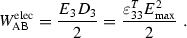  (3.47)

• $\Rightarrow$ : During this state change, the piezoelectric cylinder is electrically loaded with a resistor R. Besides, we prohibit mechanical movements in thickness directions, which can be arranged by an appropriate clamping of the cylinder. Consequently, $S_3$ stays constant and the mechanical stress $T_3$ changes. At state , the state variables are given by

  $$\begin{aligned} \begin{array}{lll}\displaystyle S_3&{}=S_{\mathrm {max}}=d_{33} E_{\mathrm {max}} \qquad \qquad &{}T_3=T_{\mathrm {max}} = \displaystyle \frac{d_{33} E_{\mathrm {max}}}{s_{33}^E} \nonumber \\ D_3&{}=D_{\mathrm {max}}\!=d_{33} T_{\mathrm {max}} \qquad \qquad \! &{}E_3=0 \;. \nonumber \end{array} \end{aligned}$$

  Since stresses occur in the cylinder, there is a remaining flux density (i.e., $D_3\ne 0$) on the electrodes at state . The electrical energy (per unit volume) released by the resistor results in

  

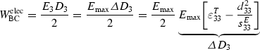  (3.48)

  with flux density change $\varDelta D_3$ from state to state . Similar to the previous conversion direction, we are able to simplify this relation by using the parameter conversion $\varepsilon _{33}^S=\varepsilon _{33}^T-d_{33}^2/s_{33}^E$ (see (3.33)) to

  

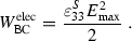  (3.49)

• $\Rightarrow$ : At the end of the conversion cycle, we return to state by removing the mechanical clamping. Furthermore, the piezoelectric cylinder is electrically unloaded. Finally, the state variables become

  $$\begin{aligned} S_3&=0 \qquad \qquad \! \,\,T_3=0 \nonumber \\ D_3&=0 \qquad \qquad E_3=0 \;. \nonumber \end{aligned}$$

  During this state change, the mechanical energy per unit volume that is released from the cylinder computes as

  

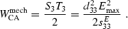  (3.50)

Again, we take into account the energy balance for the entire conversion cycle. The piezoelectric cylinder is electrically loaded from state to state with . Subsequently, the cylinder releases  from state to state leading to the stored energy

(3.51)

which has to correspond to the released mechanical energy  from state into state . This can also be seen from the parameter equation $\varepsilon _{33}^T - \varepsilon _{33}^S=d_{33}^2/s_{33}^E$. The electromechanical coupling factor $k_{33}$ characterizing the conversion from electrical into mechanical energy reads as

(3.52)

As the comparison of (3.46) and (3.52) reveals, $k_{33}$ is identical for both directions of energy conversion. In other words, it does not matter for conversion efficiency if mechanical energy is converted into electrical energy or vice versa. Note that this is an essential property of the piezoelectric coupling mechanism.

Apart from $k_{33}$, we can deduce various other electromechanical coupling factors for piezoelectric materials. For the crystal class 6mm, $k_{31}$ and $k_{15}$ are such factors that relate to the transverse and transverse shear mode of piezoelectricity, respectively. These electromechanical coupling factors are given by ($s_{44}^E=s_{55}^E$)

$$\begin{aligned} k_{31}^2=\frac{d_{31}^2}{\varepsilon _{33}^T s_{11}^E} \qquad \text {and} \qquad k_{15}^2=\frac{d_{15}^2}{\varepsilon _{11}^T s_{55}^E} \;. \end{aligned}$$

(3.53)

Depending on the piezoelectric material, the electromechanical coupling factors differ significantly. For instance, several piezoceramic materials offer remarkable values for $k_{33}$, $k_{31}$, and $k_{15}$. On the other hand, certain materials (e.g., cellular polymers) provide large values for $k_{33}$ but only a small coupling factor $k_{31}$.

3.6 Piezoelectric Materials

Piezoelectric materials exhibit either a crystal structure or, at least, areas with a crystal-like structure. In general, a crystal is characterized by a periodic repetition of the atomic lattice structure in all directions of space. The smallest repetitive part of the crystal is termed unit cell. Depending on the symmetry properties of the unit cell, we can distinguish between 32 crystal classes that are also termed crystallographic point groups  (see Fig. 3.8) [28, 42]. Piezoelectric properties will only arise when the structure of the unit cell is asymmetric. 21 out of the 32 crystal classes fulfill this property because they are noncentrosymmetric which means that they do not have a center of symmetry. 20 out of these 21 crystal classes show piezoelectricity. While 10 crystal classes are pyroelectric, the remaining 10 crystal classes are nonpyroelectric. The 20 piezoelectric crystal classes can be grouped into the seven crystal systems: triclinic, monoclinic, orthorhombic, tetragonal, rhombohedral, hexagonal, and cubic crystal system. Table 3.3 contains the abbreviations of the 20 piezoelectric crystal classes according to the Hermann–Mauguin notation. As a matter of course, the material tensors (e.g., $\left[ {\mathbf {d}} \right]$, $\left[ {\varvec{\varepsilon }^T} \right]$ and $\left[ {\mathbf {s}^E} \right]$ in d-form) of piezoelectric materials differ for the crystal classes regarding the number of independent material parameters as well as the entries being nonzero.

Fig. 3.8

Classification of the 32 crystal classes (crystallographic point groups)

Table 3.3 Abbreviations of piezoelectric crystal classes according to Hermann–Mauguin notation; crystal classes grouped into seven crystal systems

The choice of the used piezoelectric material always depends on the applications. Several piezoelectric sensors and actuators call for materials that provide high piezoelectric strain constants $d_{ip}$ and high electromechanical coupling factors. A wide variety of applications demand piezoelectric materials that are free from hysteretic behavior and offer high mechanical stiffness, i.e., small values for the elastic compliance constants $s_{pq}^E$. On the other hand, there also exist applications requiring mechanically flexible materials with piezoelectric properties. It is, therefore, impossible to find a piezoelectric material that is most appropriate for all kinds of piezoelectric sensors and actuators. However, for each application, one can define a specific figure of merit, which comprises selected material parameters. In the following, we will study different piezoelectric materials, their main properties, and the manufacturing process. This includes single crystals such as quartz (see Sect. 3.6.1), polycrystalline ceramic materials such as lead zirconate titanate (see Sect. 3.6.2) and polymers such as PVDF (see Sect. 3.6.3).

3.6.1 Single Crystals

There exists a large number of piezoelectric single crystals. In general, they can be divided into naturally occurring (e.g., quartz) and synthetically produced materials (e.g., lithium niobate). Table 3.4 lists well-known representatives for both groups including chemical formulas as well as crystal classes. Below, we will concentrate on quartz because this piezoelectric single crystal plays still an importance role in practical applications like piezoelectric sensors. The reason for its importance is not least due to the possibility that quartz can be manufactured synthetically by artificial growth. Furthermore, lithium niobate will be briefly discussed since such piezoelectric single crystals are often utilized in surface acoustic wave (SAW) devices. At the end, a short introduction to relaxor-based single crystals is given.

Table 3.4 Chemical formula and crystal class of selected naturally occurring and synthetically produced piezoelectric single crystals

Quartz

Quartz crystals at room temperature are commonly named $\alpha$-quartz. At the temperature of $573\,{}^\circ \mathrm{C}$, a structural phase transition takes place inside the quartz crystal, which is stable in the temperature range from $573\,{}^\circ \mathrm{C}$ to $870\,{}^\circ \mathrm{C}$. The resulting crystal is named $\beta$-quartz and differs considerably from the $\alpha$-quartz [14, 42]. This does not only refer to the material parameters but also to the crystal class. $\alpha$- and $\beta$-quartzes belong to crystal class 32 and 622, respectively. Since the temperatures in most of the practical applications are below $500\,{}^\circ \mathrm{C}$, let us study $\alpha$-quartzes in more detail. In the d-form, the material tensors of the crystal class 32 feature the structure

(3.54)

(3.55)

and, thus, contain altogether 10 independent entries.

$\alpha$-quartz exists in two crystal shapes, namely the left-handed and right-handed $\alpha$-quartz. The naming originates from the rotation of linearly polarized light that propagates through the quartz crystal along its optical axis. While right-handed quartzes rotate the polarization plane clockwise, left-handed quartzes perform a counterclockwise rotation. The difference of both shapes also appears in the sign of the material parameters, e.g., $d_{14}$ is positive for a left-handed $\alpha$-quartz and negative for a left-handed $\alpha$-quartz. Figure 3.9 illustrates the fundamental structure of a left-handed $\alpha$-quartz, whereby the z-axis coincides with the optical axis of the crystal.

Fig. 3.9

Fundamental structure of left-handed $\alpha$-quartz

It seems only natural that $\alpha$-quartzes in the original structure as shown in Fig. 3.9 cannot be used in piezoelectric devices. Owing to this fact, one has to cut out parts such as thin slices. The most well-known cuts are listed hereinafter [14, 28].

• X-cut: plate perpendicular to x-axis.

• Y-cut: plate perpendicular to y-axis.

• Z-cut: plate perpendicular to z-axis.

• Rotated Y-cuts: plate perpendicular to yz-plane.

By means of these cuts, it is possible to create piezoelectric elements, which offer distinct modes of piezoelectricity. For example, the X-cut will lead to the longitudinal mode if the cutted plate is covered with electrodes at the top and bottom surface.

Even though quartz is one of the most frequent minerals on earth, the great demand for quartz crystals in desired size and quality makes synthetic production indispensable. Synthetic quartz crystal can be artificially grown by the so-called hydrothermal method  [21, 24]. Thereby, the crystal growth is conducted in a thick-walled autoclave at very high pressure up to $200\,\mathrm{{MPa}}$ and temperatures of $\approx$400$\,{}^\circ \mathrm{C}$. Water with a small amount of sodium carbonate (chemical formula Na$_{\mathrm {2}}$CO$_{\mathrm {3}}$) or sodium hydroxide (chemical formula NaOH) serves as a solvent. The synthetic production of quartz crystals weighting more than $1\,\mathrm{{kg}}$ takes several weeks.

Quartz crystals are often used as piezoelectric elements in practical applications (e.g., for force and torque sensors; see Sect. 9.1) because such single crystals offer a high mechanical rigidity as well as a high electric insulation resistance. They are almost free of hysteresis and allow an outstanding linearity in practical use. Moreover, there exist temperature-compensated cuts that exhibit constant material parameters over a wide temperature range. Compared to other piezoelectric material like piezoceramic materials, quartz crystals provide, however, only small piezoelectric strain constants $d_{ip}$. This is a big disadvantage regarding efficient piezoelectric actuators. Besides, piezoelectric elements cannot be cut out from quartz crystals in any shape. The main material parameters of a left-handed $\alpha$-quartz are listed in Table 3.5.

Table 3.5 Decisive material parameters of selected piezoelectric materials; material density $\varrho _0$ in $10^3\,\mathrm{{kg}}\,{\mathrm{m}^{-3}}$; elastic compliance constants $s_{pq}^E$ in $10^{-12}\,\mathrm{{m}}\,\mathrm{{N}^{-2}}$; relative permittivity $\varepsilon _{ii}^T / \varepsilon _0$; piezoelectric strain constants $d_{ip}$ in $10^{-12}\,\mathrm{{m}}\,\mathrm{{V}^{-1}}$; table entries ‘−’ irrelevant; given data represent averaged values from literature and manufacturer [5, 10, 14, 30, 35, 42]

Lithium Niobate

Lithium niobate is a well-known synthetically produced piezoelectric single crystal, which exhibits a high Curie temperature  $\vartheta _{\mathrm {C}}$ of $1210\,{}^\circ \mathrm{C}$. That is the reason why this piezoelectric single crystal is mainly used for high-temperature sensors and ultrasonic transducers [2, 42]. Lithium niobate belongs to the crystal class 3m. In the d-form, the material tensors of this crystal class are given by

(3.56)

(3.57)

and, thus, contain altogether 13 independent entries.

Single crystals of lithium niobate can be artificially grown with the aid of the so-called Czochralski process  [8]. This manufacturing process starts with the molten state of the desired material (i.e., here lithium niobate), which is placed in a melting pot. In a next step, a slowly rotating metal rod with a seed crystal at its lower end gets immersed from above into the melt. If the seed crystal is immersed in the right way, a homogeneous boundary layer will develop between the melt and the crystal’s solid part. Subsequently, the rotating combination of metal rod and seed crystal has to be slowly pulled upwards. During this step, the melt solidifies at the boundary layer, which leads to crystal growth. By varying the rate of pulling and rotation, one can extract long single crystals that are commonly named ingots. The resulting single crystals of lithium niobate are finally brought into the desired shape through suitable crystal cuts, e.g., X-cut.

In comparison with quartz crystals, lithium niobate crystals provide significantly higher piezoelectric strain constants $d_{ip}$. Typical material parameters are listed in Table 3.5.

Relaxor-Based Single Crystals

As mentioned in Sect. 3.4.1, relaxor ferroelectrics offer pronounced electrostriction. Relaxor-based single crystals are based on such materials. Nowadays, solid solutions of lead magnesium niobate and lead titanate  (PMN-PT) as well as solid solutions of lead zinc niobate and lead titanate (PZN-PT) represent the most widely studied material compositions for relaxor-based single crystals [33, 48]. The chemical formulas of both material compositions read as

• PMN-PT: (1-x)Pb(Mg$_{\mathrm {1/3}}$Nb$_{\mathrm {2/3}}$)O$_{\mathrm {3}}$ – xPbTiO$_{\mathrm {3}}$ and

• PZN-PT: (1-x)Pb(Zn$_{\mathrm {1/3}}$Nb$_{\mathrm {2/3}}$)O$_{\mathrm {3}}$ – xPbTiO$_{\mathrm {3}}$,

whereby x ranges from 0 to 1. In principle, these material compositions can be used for polycrystalline ceramic materials (see Sect. 3.6.2). The resulting piezoceramic materials show excellent piezoelectric properties like high piezoelectric strain constants $d_{ip}$. However, by growing single crystals, the available properties are improved significantly. Crystal growth of PMN-PT and PZN-PT is often conducted by the high-temperature flux technique and the Bridgman growth technique  [23, 25, 26]. After growing, the single crystals have to be polarized in an appropriate direction.

The electromechanical coupling factor $k_{33}$ of PMN-PT and PZN-PT single crystals usually exceeds 0.9. In case of special material compositions and additional doping, one can reach extremely high electric permittivities as well as $d_{33}$-values $>2000\,\mathrm{{pm}}\,\mathrm{{V}^{-1}}$. These outstanding properties are responsible for the great interest in PMN-PT and PZN-PT single crystals for practical applications [6, 18], e.g., they should be ideal candidates for efficient piezoelectric components in ultrasonic transducers.

3.6.2 Polycrystalline Ceramic Materials

Polycrystalline ceramic materials are the most important piezoelectric materials for practical applications because they offer outstanding piezoelectric properties. Moreover, several of these so-called piezoceramic materials can be manufactured in a cost-effective manner. Barium titanate and lead zirconate titanate  (PZT) represent two well-known solid solutions that belong to the group of piezoceramic materials. Hereafter, we will discuss the manufacturing process, the basic molecular structure, the poling process, and the hysteretic behavior of piezoceramic materials. The focus lies on PZT since it is frequently used in practical applications. At the end, a brief introduction to lead-free piezoceramic materials will be given.

Manufacturing Process

The manufacturing process of piezoceramic materials mostly comprises six successive main steps, namely (i) mixing, (ii) calcination, (iii) forming, (iv) sintering, (v) applying of electrodes, and (vi) poling [12, 17]. At the beginning, powders of the raw materials (e.g., zirconium) are mixed. The powder mixture gets then heated up to temperatures between 800 and $900\,{}^\circ \mathrm{C}$ during calcination. Thereby, the raw materials react chemically with each other. The resulting polycrystalline substance is ground and mixed with binder. Depending on the desired geometry of the piezoelectric element, there exist various processes for forming. The most widely used process is cold pressing. During the subsequent sintering, the so-called green body gets bound as well as compressed at temperatures of $\approx$1200$\,{}^\circ \mathrm{C}$. To achieve a higher material density, sintering is commonly carried out in an oxygen atmosphere. The sintered blanks are, sometimes, cut and polished. In the fifth step, the blanks get equipped with electrodes. This can be done by either screen printing or sputtering. The obtained materials are usually referred to as unpolarized ceramics . The poling as final process step yields the piezoceramic material, i.e., a ceramic material featuring piezoelectric properties. Poling is usually carried out by applying strong electric fields in the range of 2–8$\,\mathrm{{k}\,\mathrm{V}\,\mathrm{{mm}^{-1}}}$ in a heated oil bath. Alternatively, one can use corona discharge for poling.

It is possible to produce various shapes of piezoceramic elements by means of the common manufacturing process. Piezoceramic disks, rings, plates, bars as well as cylinders are standard shapes of piezoceramic elements. However, slightly modified manufacturing processes additionally allow the production of other shapes like thin piezoceramic fibers that can be used for piezoelectric composite transducers (see Sect. 7.4.3). With the aid of screen printing, physical vapor deposition (e.g., sputtering), chemical vapor deposition (e.g., metal-organic CVD) as well as chemical solution deposition (e.g., solution-gelation), one can also generate films of piezoceramic materials [4, 16, 31, 43].

Molecular Structure

Piezoceramic materials such as barium titanate and PZT consist of countless crystalline unit cells, which exhibit the so-called perovskite structure , being named after the mineral perovskite [17]. In general, piezoceramic materials featuring this structure can be described by the chemical formula ABO$_{\mathrm {3}}$. While A and B are two cations (i.e., positive ions) of different size, O$_{\mathrm {3}}$ is an anion (i.e., negative ion) that bonds to both. The large cations A are located on the corners of the unit cell and the oxygen anions O$_{\mathrm {3}}$ in the center of the faces, respectively. Depending on the state of the unit cell, the small cation B is located in or close to the center. The edge lengths of a unit cell amounts a few angstroms Å ($1\,$Å$\,\widehat{=} \,0.1\,\mathrm{{nm}}$).

The unit cells of many piezoceramic materials take predominantly one of four phases, namely (i) the cubic, (ii) the tetragonal, (iii) the orthorhombic, or (iv) the rhombohedral phase  (see Fig. 3.10). In the cubic phase, the center $\mathcal {C}_{\mathrm {Q+}}$ of positive charges (cations) geometrically coincides with the center $\mathcal {C}_{\mathrm {Q-}}$ of negative charges (anions). A single unit cell behaves, thus, electrically neutral. Note that this paraelectric phase of the unit cells only exists above the Curie temperature  $\vartheta _{\mathrm {C}}$. When the temperature falls below $\vartheta _{\mathrm {C}}$, the cubic unit cell will undergo a phase transition from cubic to another phase, i.e., to the tetragonal, the orthorhombic, or the rhombohedral phase. Thereby, the unit cell gets deformed. For example, the deformation from the cubic to the tetragonal phase is $\varDelta l_{\mathrm {U}}$ in a single direction. In any case, the small cation B leaves the center of the unit cell. Consequently, $\mathcal {C}_{\mathrm {Q+}}$ does not geometrically coincide with $\mathcal {C}_{\mathrm {Q-}}$ anymore. That is the reason why there arises a dipole moment, which is termed spontaneous electric polarization  $\mathbf {p}_n$. If the positive charges amount overall $q_n$ and the distance from $\mathcal {C}_{\mathrm {Q-}}$ to $\mathcal {C}_{\mathrm {Q+}}$ is defined by the vector $\mathbf {r}_n$, the spontaneous polarization of a single unit cell will become $\mathbf {p}_n=q_n \mathbf {r}_n$.

Fig. 3.10

Unit cell of perovskite structure ABO$_{\mathrm {3}}$ in a cubic phase, b tetragonal phase, c orthorhombic phase, and d rhombohedral phase; spontaneous electric polarization $\mathbf {p}_n$; edge lengths $a_{\mathrm {U}}$, $b_{\mathrm {U}}$ and $c_{\mathrm {U}}$ of unit cell

The direction of the spontaneous electric polarization $\mathbf {p}_n$ inside a unit cell differs for the individual phases. With regard to the local coordinate system of a unit cell, $\mathbf {p}_n$ exhibits different proportions in x-, y- and z-direction. The so-called Miller index [hkl] describes the direction of $\mathbf {p}_n$ in the local coordinate system [28, 42]. For the tetragonal, the orthorhombic and the rhombohedral phase, the Miller index takes the form [001], [011], and [111], respectively. During the phase transition from the cubic to the tetragonal phase, the central cation B can move into six directions. This is accompanied by 6 possible directions of $\mathbf {p}_n$ in a global coordinate system. In contrast, there exist 8 possible directions for the rhombohedral phase and 12 possible directions for the orthorhombic phase. The total electric polarization $\mathbf {P}$ of a piezoceramic element containing N unit cells results from the vectorial sum of all spontaneous electric polarizations related to the element’s volume V, i.e.,

$$\begin{aligned} \mathbf {P} = \frac{1}{V} \sum \limits _{n=1}^N \mathbf {p}_n = \frac{1}{V} \sum \limits _{n=1}^N q_n \mathbf {r}_n \;. \end{aligned}$$

(3.58)

Here, the individual polarizations $\mathbf {p}_n$ of the unit cells have to be regarded in a global coordinate system.

Phase diagrams represent an appropriate way to illustrate the phases of piezoceramic materials with respect to both temperature $\vartheta$ and material composition. Figure 3.11 illustrates the phase diagram of PZT, which features the chemical formula Pb(Ti$_{\mathrm {x}}$Zr$_{\mathrm {1-x}}$)O$_{\mathrm {3}}$ [17, 40]. The abscissa starts with pure PbZrO$_{\mathrm {3}}$ and ends with pure PbTiO$_{\mathrm {3}}$. In between, the molar amount x of PbTiO$_{\mathrm {3}}$ increases linearly. Since the cubic phase is dominating above the Curie temperature $\vartheta _{\mathrm {C}}$, PZT does not behave like a piezoelectric material for temperatures $\vartheta >\vartheta _{\mathrm {C}}$. It can also be seen that $\vartheta _{\mathrm {C}}$ increases with increasing x. According to Fig. 3.11, there exist three stable phases of the unit cells below $\vartheta _{\mathrm {C}}$. The tetragonal phase and rhombohedral phase of PZT are also named ferroelectric phases, while the orthorhombic phase that dominates for high contents of zirconium is referred to as antiferroelectric phase. The phase boundary between the rhombohedral and tetragonal phase is of great practical importance. In the vicinity of this phase boundary, which is termed morphotropic phase boundary, a PZT element contains roughly the same number of unit cells in rhombohedral and tetragonal phase. The almost equal distribution of both phases is frequently assumed to be the origin for the outstanding properties of PZT like high electromechanical coupling factors. At room temperature, the morphotropic phase boundary is located at $\text {x}=48$, i.e., the chemical formula reads as Pb(Ti$_{\mathrm {48}}$Zr$_{\mathrm {52}}$)O$_{\mathrm {3}}$. A further advantage of PZT lies in the relatively low temperature dependence, which stems from the vertical progression of the morphotropic phase boundary.

Fig. 3.11

Phase diagram showing dominating phases of PZT (chemical formula Pb(Ti$_{\mathrm {x}}$Zr$_{\mathrm {1-x}}$)O$_{\mathrm {3}}$) with respect to temperature $\vartheta$ and material composition; Curie temperature $\vartheta _{\mathrm {C}}$; spontaneous electric polarization $\mathbf {p}_n$ of unit cell

Poling Process and Hysteresis

As already mentioned, piezoceramic materials consist of countless unit cells. Now, let us take a closer look at the internal structure of such materials, which is also illustrated in Fig. 3.12. Neighboring unit cells that exhibit the same directions of spontaneous electric polarization $\mathbf {p}_n$ form a so-called domain [14, 17]. Several of those domains form a single grain, which represents the smallest interrelated part of a piezoceramic material. The boundaries between neighboring grains are named grain boundaries, whereas the boundaries between neighboring domains inside a grain are termed domain walls. In the tetragonal phase, the directions of $\mathbf {p}_n$ between two neighboring domains can be differ by either 90 or $180^\circ$. By contrast, this angle can take the values 71, 109, or $180^\circ$ in case of the rhombohedral phase of PZT.

Fig. 3.12

Internal structure of piezoceramic materials; arrows indicate direction of spontaneous electric polarization $\mathbf {p}_n$ of unit cells inside single domain

It is not surprising that apart from the material composition, the current domain configuration determines the properties of a piezoceramic material. When such a material is cooled down below the Curie temperature (e.g., after sintering), the unit cells will undergo a phase transition from the cubic phase to another one. This goes hand in hand with a spontaneous electric polarization and mechanical deformations of the unit cells yielding mechanical stresses. Owing to the fact that each closed system wants to minimize its free energy (see Sect. 3.2), the unit cells align themselves in a way that both the electrical and the mechanical energy take a minimum. The resulting characteristic domain configuration (cf. Fig. 3.12) leads, thus, to a vanishing total electric polarization $\mathbf {P}$. That is the reason why the material, the unpolarized ceramics, does not offer piezoelectric properties in this state from the macroscopic point of view.

To activate the piezoelectric coupling which means $\smash {\left\| \mathbf {P} \right\| _2\ne 0}$, we have to appropriately align the unit cells and, therefore, the domains within the unpolarized ceramics. The underlying activation process is known as poling [12, 14, 17]. The alignment is mostly conducted by applying strong electric fields to the unpolarized ceramics. In doing so, the spontaneous electric polarizations $\mathbf {p}_n$ of the unit cells get aligned along the crystal axis that is nearest to the direction of the electrical field lines. The number of neighboring unit cells exhibiting the same direction of $\mathbf {p}_n$ increases which reduces the number of domains inside a single grain. This implies a growth of the still existing domains as well as a movement of the domain walls. Apart from that, the alignment of the unit cells causes a deformation of the grains, which becomes visible as mechanical strain of the piezoceramic element.

In the following, we will regard a mechanically unloaded thin piezoceramic disk, which is completely covered with electrodes at the top and bottom surface. Therefore, it is possible to reduce the vectors of electric polarization $\mathbf {P}$ and mechanical strain $\mathbf {S}$ to scalars, i.e., to P and S. Figure 3.13a and b depict $P\!\left( E \right)$ and $S\!\left( E \right)$ of the disk as a function of the applied electric field intensity E, respectively. Exemplary domain configurations for the states to are shown in Fig. 3.13c. These states are also marked in $P\!\left( E \right)$ as well as $S\!\left( E \right)$. In the initial state  (e.g., after sintering), the disk shall be unpolarized which means $P=0$. Without limiting the generality, the mechanical strain is assumed to be zero, i.e., $S=0$. The domains will get aligned when a strong positive electric field is applied. While doing so, the so-called virgin curve is passed through until the positive saturation of the electric polarization $P_{\mathrm {sat}}^+$ and the mechanical strain $S_{\mathrm {sat}}^+$ is reached at state . In this state, the spontaneous electric polarizations of the unit cells are almost perfectly aligned, which can also be seen in high values of $P_{\mathrm {sat}}^+$ and $S_{\mathrm {sat}}^+$. A further increase of E does not considerably increase both values because the intrinsic effects of electromechanical coupling (see Sect. 3.4.1) are dominating then. In contrast, steep gradients in $P\!\left( E \right)$ and $S\!\left( E \right)$ indicate extrinsic effects (see Sect. 3.4.2).

Fig. 3.13

Hysteresis curves of a electric polarization $P\!\left( E \right)$ and b mechanical strain $S\!\left( E \right)$ of piezoceramic disk; linearization refers to small-signal behavior; c exemplary domain configurations for states to  [46]

If E is reduced to zero (state ), the majority of unit cells will stay aligned, i.e., the domain configuration barely changes. Only a few unit cells belonging to unstable domains switch back to the original state, whereby P as well as S get slightly reduced. The resulting positive values at $E=0$ are termed remanent electric polarization  $P_{\mathrm {r}}^+$ and remanent mechanical strain  $S_{\mathrm {r}}^+$, respectively.⁵ When E is reduced to negative values, state will be passed through. At this state, the electric polarization of the disks equals zero, which is arranged by the negative coercive field intensity  $E_{\mathrm {c}}^-$. A further reduction of E leads to the negative saturation of the electric polarization $P_{\mathrm {sat}}^-$ and the mechanical strain $S_{\mathrm {sat}}^-$ at state . Thereby, the domains get aligned in the opposite direction to that in case of positive saturation (cf. Fig. 3.13c). The electric polarization takes, thus, the negative value of $P_{\mathrm {sat}}^+$. In contrast, $S_{\mathrm {sat}}^-$ coincides with $S_{\mathrm {sat}}^+$ because it does not make a difference for the mechanical deformation of a unit cell whether $\mathbf {p}_n$ points in positive or negative direction. The remaining parts of the curves $P\!\left( E \right)$ and $S\!\left( E \right)$ describe the same material behavior as the previous ones. State refers to the negative remanent electric polarization $P_{\mathrm {r}}^-=-P_{\mathrm {r}}^+$ and remanent mechanical strain $S_{\mathrm {r}}^+=S_{\mathrm {r}}^-$, while state with the positive coercive field $E_{\mathrm {c}}^+$ corresponds to state . Note that the initial domain configuration of state can be retrieved by heating up the piezoceramic material above the Curie temperature.

As can be seen in Fig. 3.13, piezoceramic materials exhibit a strongly pronounced hysteretic behavior, which is commonly termed ferroelectric behavior . For high electrical excitation signals, the electric polarization and mechanical strain differ, therefore, considerably for increasing and decreasing inputs, respectively. The phenomenological modeling of this large-signal behavior will be addressed in Chap. 6. Besides the ferroelectric behavior, piezoceramic materials also show ferroelastic behavior . This means for a piezoceramic disk that both the mechanical strain S and the electric polarization P are altered by the mechanical stress T. Figure 3.14a depicts exemplary curves $P\!\left( T \right)$ and $S\!\left( T \right)$ of the resulting hysteretic behavior.

Fig. 3.14

a Ferroelastic behavior of electric polarization $P\!\left( T \right)$ and mechanical strain $S\!\left( T \right)$; mechanical stress T; b hysteresis curve of $P\!\left( E \right)$ for ferroelectrically hard and soft piezoceramic materials, respectively

It seems only natural that the material composition remarkably affects the ferroelectric behavior of piezoceramic materials. By means of doping, one can change properties of piezoceramic materials such as electromechanical coupling factors in a specific manner [14, 17, 41]. A general distinction is made between acceptor doping and donor doping. In case of acceptor doping, the remanent electric polarization $\left| P_r^{\pm } \right|$, the electromechanical coupling factors and the elastic compliance constants $s_{pq}^E$ get reduced, while the coercive field intensity $\left| E_{\mathrm {c}}^\pm \right|$ increases. The opposite behavior results from donor doping of the piezoceramic material, i.e., $\left| P_r^{\pm } \right|$, the electromechanical coupling factors and $s_{pq}$ are reduced, while $\left| E_{\mathrm {c}}^\pm \right|$ decreases. In accordance with the behavior of ferromagnetic materials, acceptor and donor doping of piezoceramic materials leads to ferroelectrically hard and ferroelectrically soft materials , respectively. Figure 3.14b demonstrates the basic difference of both material types in the hysteresis curve $P\!\left( E \right)$. The larger width of the hysteresis curve of ferroelectrically hard materials stems from the lower domain wall mobility compared to ferroelectrically soft materials. Because the area within the hysteresis curve rates thermal losses, ferroelectrically hard materials usually take in piezoelectric actuators lower temperatures during operation than ferroelectrically soft materials.

Piezoelectric sensors and actuators that contain piezoceramic materials are mainly operated in the polarized state, i.e., state in Fig. 3.13a and b. The small-signal behavior refers to the linearization. We can describe the linearized behavior of almost any piezoceramic material by the constitutive equations for piezoelectric materials of crystal class 6mm (see (3.32)). Consequently, the three material tensors contain altogether 10 independent entries. The identification of these entries is detailed in Chap. 5. Typical material parameters of piezoceramic materials are listed in Table 3.5. It can be clearly seen that the piezoelectric strain constants are much higher than those of $\alpha$-quartz.

Lead-Free Materials

Most of the practically used piezoceramic materials like PZT contain a considerable amount of lead, which belongs to hazardous substances. However, the European Union has adopted the directives Waste Electrical and Electronic Equipment (WEEE) and Restriction of the use of certain Hazardous Substances in electrical and electronic equipment (RoHS) in 2003 [13]. These directives aim at protecting human health and environment by substitution of hazardous substances through safe or safer materials. Similar directives were also adopted in other countries. Some defined applications containing hazardous substances are exempt from the directives because the elimination is technically impracticable. The list of exempted applications, which is reviewed at least every four years, includes the use of lead in electronic ceramic parts such as piezoelectric devices. Nevertheless, the use will be prohibited as soon as there exists a suitable substitution for lead-based materials.

During the last two decades, there has been a lot of research to find lead-free piezoceramic materials, which provide similar performance as lead-based piezoceramic materials in practical applications. The most important lead-free piezoceramic materials are nowadays based on sodium potassium niobate, bismuth sodium titanate and bismuth potassium titanate  [11, 38, 39, 47]. The chemical formula of sodium potassium niobate takes the form K$_{\mathrm {1-x}}$Na$_{\mathrm {x}}$NbO$_{\mathrm {3}}$ (KNN or NKN). With the aid of appropriate doping and modifications of material composition, the sintering of KNN-based piezoceramic materials is facilitated. To some extent, KNN-based materials offer a piezoelectric strain constant $d_{33}>200 \,\mathrm{{pm}\,\mathrm{{V}^{-1}}}$, which is comparable to PZT. This also refers to the electromechanical coupling factors.

The chemical formula of bismuth sodium titanate and bismuth potassium titanate reads as Bi$_{\mathrm {0.5}}$Na$_{\mathrm {0.5}}$TiO$_{\mathrm {3}}$ (BNT) and Bi$_{\mathrm {0.5}}$K$_{\mathrm {0.5}}$TiO$_{\mathrm {3}}$ (BKT), respectively. Pure BNT-based and BKT-based piezoceramic materials are difficult to sinter and exhibit high coercive field intensities $\left| E_{\mathrm {c}}^{\pm } \right|$ of more than $5\,\mathrm{{kV}\,\mathrm{{mm}^{-1}}}$, which implies a complicated poling process [38]. Furthermore, they show comparatively low piezoelectric properties. Just as in case of KNN-based materials, one can modify BNT-based and BKT-based piezoceramic materials in a way that sintering is facilitated and piezoelectric properties get improved. The binary Bi-based material compositions BNT-BT, BKT-BT, and BNT-BKT as well as the ternary material compositions BNT-BT-BKT and BNT-BT-KNN represent well-known modifications. Here, BT stands for barium titanate, i.e., BaTiO$_{\mathrm {3}}$.

Although the progress in competitive KNN-based, BNT-based, and BKT-based piezoceramic materials is promising, the great breakthrough has not been made yet. This mainly stems from the costly manufacturing process and the worse piezoelectric properties compared with lead-based materials. PZT is, therefore, still dominating the market. However, lead-free piezoceramic materials are already commercially available, e.g., the BNT-based material PIC700 from the company PI Ceramic GmbH [35].

Apart from piezoelectric single crystals (e.g., quartz) and the just mentioned materials (e.g., KNN), there exists a variety of other lead-free materials, which offer piezoelectric properties. Aluminum nitride  (AlN) and zinc oxide  (ZnO) are prominent representatives for such lead-free materials. Both show a hexagonal crystal structure and belong to the group of wurtzite-structured materials  [40]. The polarization direction of AlN and ZnO is set by the crystal orientation. Regardless of whether these materials are used as single crystals or oriented polycrystalline ceramic, the polarization direction cannot be altered after the manufacturing process. That is the reason why both materials do not belong to ferroelectric materials. Compared to other lead-based piezoceramic materials, the achieved electromechanical coupling is much less pronounced. The piezoelectric strain constant $d_{33}$ of AlN and ZnO amounts $\approx$5$\,\mathrm{{pm}\,\mathrm{{V}^{-1}}}$ and $\approx$10$\,\mathrm{{pm}\,\mathrm{{V}^{-1}}}$, respectively [34]. Nevertheless, by modified material compositions like scandium aluminum nitride  (chemical formula Sc$_{\mathrm {x}}$Al$_{\mathrm {1-x}}$N), $d_{\mathrm {33}}$ reaches values >20$\,\mathrm{{pm}\,\mathrm{{V}^{-1}}}$ [1, 29]. AlN and its modifications can be sputter-deposited on silicon substrates at moderate temperatures [27]. Because this procedures allows the fabrication of thin piezoelectric films with thicknesses less than $100\,\mathrm{{nm}}$, AlN-based materials are often utilized in micro electromechanical systems  (MEMS).

3.6.3 Polymers

There exist some polymers, which show piezoelectric properties after activation. If such polymers are produced in thin foils, they can be used as mechanically flexible piezoelectric sensors and actuators. Below, we will concentrate on two piezoelectric polymers, namely polyvinylidene fluoride (PVDF) and cellular polypropylene.

PVDF

PVDF materials consist of long-chain molecules (see Fig. 3.15a) that are alternately composed of methylene (chemical formula CH$_{\mathrm {2}}$) and fluorocarbon (chemical formula CF$_{\mathrm {2}}$) [36, 44]. Partly, the chain molecules are arranged in thin lamellar crystal-like structures (see Fig. 3.15b). The remaining chain molecules are irregularly arranged which leads to amorphous regions. PVDF belongs, therefore, to the group of semi-crystalline piezoelectric polymers. Inside a single lamellar crystal-like structure, the dipole moments of the molecules point in the same direction. However, since the lamellar crystal-like structures are orientated randomly, PVDF does not offer piezoelectric properties in the initial state.

Fig. 3.15

a Chain molecules CH$_{\mathrm {2}}$ and CF$_{\mathrm {2}}$ of PVDF; b arrangement of chain molecules within PVDF material [22]; dipole moments inside lamellar crystal-like structures point in same direction

PVDF can be synthesized from the gaseous vinylidene fluoride via a free-radical polymerization [9]. The polymerization process takes place in suspensions and emulsions at temperatures from 10–150$\,{}^\circ \mathrm{C}$ and pressures up to $30\,\mathrm{{MPa}}$. Melt casting, solution casting, and spin coating represent typical subsequent process steps. The result of the manufacturing process is usually a PVDF film with a thickness in the range of a few microns up to more than $100\,\upmu \mathrm{{m}}$.

Just as in case of polycrystalline ceramic materials, one has to activate the electromechanical coupling of PVDF films with the aid of an appropriate poling process [14, 36]. The basic idea of poling lies in aligning the lamellar crystal-like structures and, thus, in aligning the dipole moments. When the PVDF film is equipped with electrodes, this can be conducted by applying high electric field intensities up to $100\,\mathrm{{kV}\,\mathrm{{mm}^{-1}}}$. The process should be carried out in a heated vacuum chamber or inside an electrically insulating fluid to avoid electrical breakdowns. Poling of PVDF materials is also possible by exploiting corona discharge. In the course of this, the film does not have to be equipped with electrodes. Regardless of the used process, mechanical stretching of PVDF during poling enhances the alignment of the lamellar crystal-like structures and, therefore, the piezoelectric properties get improved. Similar to polycrystalline ceramic materials, PVDF exhibits a certain hysteretic large-signal behavior of the total electric polarization and mechanical strain. That is the reason why PVDF is a ferroelectric polymer.

The piezoelectric properties of PVDF materials are less pronounced than of piezoceramic materials like PZT. Typically, uniaxially stretched PVDF films provide the piezoelectric strain constants $d_{33}\approx - 20\,\mathrm{{pm}\,\mathrm{{V}^{-1}}}$ and $d_{31}\approx 15\,\mathrm{{pm}\,\mathrm{{V}^{-1}}}$ [14]. Note that the signs of $d_{33}$ and $d_{31}$ differ from those of other piezoelectric materials (see Table 3.5). The relative electric permittivity and the electromechanical coupling factors of PVDF films amount $\varepsilon _{\mathrm {r}}=12$, $k_{33}\approx 0.3$ and $k_{31}\approx 0.1$ [36]. Copolymers of PVDF with trifluoroethylene (P(VDF-TrFE)) offer slightly higher $\left| d_{ip} \right|$-values and better electromechanical coupling factors. The comparatively large piezoelectric voltage constant $g_{33}\approx 0.2\,\mathrm{{V}\,\mathrm{m}\,\mathrm{{N}^{-1}}}$ and low acoustic impedance⁶ of $Z_{\mathrm {aco}}\approx 4\cdot 10^6\,{\mathrm{N}\,\mathrm{s}\,\mathrm{{m}}^{-3}}$ make PVDF films interesting as broadband piezoelectric components for hydrophones and ultrasonic transducers (see, e.g., Sect. 8.1.1).

Cellular Polypropylene

Cellular polypropylene (PP) is currently the best-known representative of the so-called cellular ferroelectrets , which are also termed cellular piezoelectrets and voided charged polymers  [3, 36]. It features piezoelectric properties after an appropriate activation procedure. The conventional manufacturing process of cellular PP films starts with inclusions such as air or small grains of sand, which are blown into PP in the molten state. During the following cooling, spherical cavities with approximately $10\,\upmu \mathrm{{m}}$ in diameter emerge around the inclusions. The modified PP material is, subsequently, heated up and extruded in films of 70–100$\,\upmu \mathrm{{m}}$ thickness by means of two-dimensional shaking motions below atmospheric pressure. In doing so, the spherical cavities get deformed to lenticular voids with diameters ranging from $10\,\upmu \mathrm{{m}}$ up to $100\,\upmu \mathrm{{m}}$ and heights in the range of 2–10$\,\upmu \mathrm{{m}}$ (see Fig. 3.16a). The surface roughness of the PP film is minimized by sealing both the top and bottom surface with homogeneous PP. The geometric dimensions of the lenticular voids (especially their height) are often additionally increased by exposing the PP film to a remarkable overpressure (e.g., $2\,\mathrm{{MPa}}$) for several hours [45, 49]. When the overpressure is rapidly reduced, the size of the voids will increase permanently.

Fig. 3.16

a Scanning electron micrograph of PP film; b charge distribution inside PP film at interface of lenticular voids and surrounding PP [37]

To activate electromechanical coupling in the resulting PP film, corona discharge is usually applied for poling. This procedure leads to permanent electric charges arising at the interfaces of lenticular voids and surrounding PP (see Fig. 3.16b). Since the electric charges exhibit opposite signs at the top and bottom surface of the interfaces, an electric field is generated inside the voids. The electric field yields an electrostatic force, which reduces the void heights. The film thickness gets, thus, slightly reduced during poling. In the final step of the manufacturing process, the top and bottom surface of the PP film is metallized with thin layers (e.g., aluminum) that serve as electrodes. The reason for the piezoelectric properties of polarized PP films lies in the fact that each charged lenticular void represents a dipole with a certain dipole moment. Just as several other piezoelectric materials, PP films also show a hysteretic large-signal behavior.

A well-established cellular PP film for piezoelectric transducers is the electromechanical film  (EMFi) material, which is produced by the company Emfit Ltd [7, 32]. The piezoelectric strain constant $d_{33}$ of PP films can reach values of more than $600\,\mathrm{{pm}\,\mathrm{{V}^{-1}}}$, which is comparable to piezoceramic materials (see Table 3.5). In contrast, $d_{31}$ takes extremely low values. Both the relative electric permittivity and the electromechanical coupling factor $k_{33}\approx 0.1$ of PP films are much smaller than that of piezoceramic materials and PVDF. Nevertheless, PP films are well suited for airborne ultrasonic transducers (see Sect. 7.6.1). Besides the high $d_{33}$-value, this can be ascribed to the outstanding piezoelectric voltage constant $g_{33}\approx 30\,{\mathrm{V}\,\mathrm{m}\,\mathrm{{N}}^{-1}}$ and the extremely small acoustic impedance $Z_{\mathrm {aco}}\approx 3\cdot 10^4\,{\mathrm{N}\,\mathrm{s}\,\mathrm{{m}}^{-3}}$ of cellular PP. The main problem of conventional PP films in practical applications lies in the strongly pronounced temperature sensitivity because temperatures higher than $60\,{}^\circ \mathrm{C}$ cause an irreversible change of the piezoelectric properties. However, it is possible to relocate this change to higher temperatures by using cellular ferroelectrets that are based on layered structures of polytetrafluoroethylene (PTFE ) and fluoroethylenepropylene (FEP ) [50]. The resulting cellular fluorocarbon film shows $d_{33}$-values of almost $600\,\mathrm{{pm}\,\mathrm{{V}^{-1}}}$ at a temperature of $120\,{}^\circ \mathrm{C}$.

References

Akiyama, M., Kamohara, T., Kano, K., Teshigahara, A., Takeuchi, Y., Kawahara, N.: Enhancement of piezoelectric response in scandium aluminum nitride alloy thin films prepared by dual reactive cosputtering. Adv. Mater. 21(5), 593–596 (2009)
Baba, A., Searfass, C.T., Tittmann, B.R.: High temperature ultrasonic transducer up to 1000 \(^{\circ }\)C using lithium niobate single crystal. Appl. Phys. Lett. 97(23) (2010)
Bauer, S., Gerhard-Multhaupt, R., Sessler, G.M.: Ferroelectrets: soft electroactive foams for transducers. Phys. Today 57(2), 37–43 (2004)
Budd, K.D., Dey, S.K., Payne, D.A.: Sol-gel processing of PbTiO3, PbZrO3, PZT, and PLZT thin films. Br. Ceram. Proc. 36, 107–121 (1985)
CeramTec GmbH: Product portfolio (2018). https://www.ceramtec.com
Chen, Y., Lam, K.H., Zhou, D., Yue, Q., Yu, Y., Wu, J., Qiu, W., Sun, L., Zhang, C., Luo, H., Chan, H.L.W., Dai, J.: High performance relaxor-based ferroelectric single crystals for ultrasonic transducer applications. Sensors (Switzerland) 14(8), 13730–13758 (2014)
Emfit Ltd: Manufacturer of electro-mechanical films (2018). https://www.emfit.com
Evers, J., Klüfers, P., Staudigl, R., Stallhofer, P.: Czochralski’s creative mistake: a milestone on the way to the gigabit era. Angewandte Chemie - International Edition 42(46), 5684–5698 (2003)
Gallantree, H.R.: Review of transducer applications of polyvinylidene fluoride. IEE Proc. I: Solid State Electron Devices 130(5), 219–224 (1983)
Gautschi, G.: Piezoelectric Sensorics. Springer, Heidelberg (2002)
Guo, Y., Kakimoto, K.I., Ohsato, H.: Phase transitional behavior and piezoelectric properties of (Na0.5K0.5)NbO3-LiNbO3 ceramics. Appl. Phys. Lett. 85(18), 4121–4123 (2004)
Haertling, G.H.: Ferroelectric ceramics: History and technology. J. Am. Ceram. Soc. 82(4), 797–818 (1999)
Hedemann-Robinson, M.: The EU directives on waste electrical and electronic equipment and on the restriction of use of certain hazardous substances in electrical and electronic equipment: adoption achieved. Eur. Environ. Law Rev. 12(2), 52–60 (2003)
Heywang, W., Lubitz, K., Wersing, W.: Piezoelectricity: Evolution and Future of a Technology. Springer, Heidelberg (2008)
Ikeda, T.: Fundamentals of Piezoelectricity. Oxford University Press (1996)
Izyumskaya, N., Alivov, Y.I., Cho, S.J., Morkoç, H., Lee, H., Kang, Y.S.: Processing, structure, properties, and applications of PZT thin films. Crit. Rev. Solid State Mater. Sci. 32(3–4), 111–202 (2007)
Jaffe, B., Cook, W.R., Jaffe, H.: Piezoelectric Ceramics. Academic Press Limited (1971)
Jiang, X., Kim, J., Kim, K.: Relaxor-PT single crystal piezoelectric sensors. Crystals 4(3), 351–376 (2014)
Kaltenbacher, M.: Numerical Simulation of Mechatronic Sensors and Actuators - Finite Elements for Computational Multiphysics, 3rd edn. Springer, Heidelberg (2015)
Kamlah, M., Böhle, U.: Finite element analysis of piezoceramic components taking into account ferroelectric hysteresis behavior. Int. J. Solids Struct. 38(4), 605–633 (2001)
Laudise, R.A., Nielsen, J.W.: Hydrothermal crystal growth. Solid State Phys. - Adv. Res. Appl. 12(C), 149–222 (1961)
Lerch, R., Sessler, G.M., Wolf, D.: Technische Akustik: Grundlagen und Anwendungen. Springer, Heidelberg (2009)
Li, X., Luo, H.: The growth and properties of relaxor-based ferroelectric single crystals. J. Am. Ceram. Soc. 93(10), 2915–2928 (2010)
Liebertz, J.: Synthetic precious stones. Angewandte Chemie International Edition in English 12(4), 291–298 (1973)
Lim, L.C., Shanthi, M., Rajan, K.K., Lim, C.Y.H.: Flux growth of high-homogeneity PMN-PT single crystals and their property characterization. J. Cryst. Growth 282(3–4), 330–342 (2005)
Luo, J., Zhang, S.: Advances in the growth and characterization of relaxor-pt-based ferroelectric single crystals. Crystals 4(3), 306–330 (2014)
Martin, F., Muralt, P., Dubois, M.A., Pezous, A.: Thickness dependence of the properties of highly c-axis textured ain thin films. J. Vac. Sci. Technol. A: Vac. Surf. Films 22(2), 361–365 (2004)
Mason, W.P.: Piezoelectric Crystals and Their Application to Ultrasonics. D. van Nostrand, New York (1949)
Mayrhofer, P.M., Euchner, H., Bittner, A., Schmid, U.: Circular test structure for the determination of piezoelectric constants of ScxAl1-xN thin films applying Laser Doppler Vibrometry and FEM simulations. Sens. Actuators A: Phys. 222, 301–308 (2015)
Meggitt Sensing Systems: Product portfolio (2018). https://www.meggittsensingsystems.com
Muralt, P., Kohli, M., Maeder, T., Kholkin, A., Brooks, K., Setter, N., Luthier, R.: Fabrication and characterization of PZT thin-film vibrators for micromotors. Sens. Actuators A: Phys. 48(2), 157–165 (1995)
Paajanen, M., Lekkala, J., Kirjavainen, K.: Electromechanical Film (EMFi) - a new multipurpose electret material. Sens. Actuators A: Phys. 84(1), 95–102 (2000)
Park, S.E., Shrout, T.R.: Ultrahigh strain and piezoelectric behavior in relaxor based ferroelectric single crystals. J. Appl. Phys. 82(4), 1804–1811 (1997)
Patel, N.D., Nicholson, P.S.: High frequency, high temperature ultrasonic transducers. NDT Int. 23(5), 262–266 (1990)
PI Ceramic GmbH: Product portfolio (2018). https://www.piceramic.com
Ramadan, K.S., Sameoto, D., Evoy, S.: A review of piezoelectric polymers as functional materials for electromechanical transducers. Smart Mater. Struct. 23(3) (2014)
Rupitsch, S.J., Lerch, R., Strobel, J., Streicher, A.: Ultrasound transducers based on ferroelectret materials. IEEE Trans. Dielectr. Electr. Insul. 18(1), 69–80 (2011)
Rödel, J., Jo, W., Seifert, K.T.P., Anton, E.M., Granzow, T., Damjanovic, D.: Perspective on the development of lead-free piezoceramics. J. Am. Ceram. Soc. 92(6), 1153–1177 (2009)
Rödel, J., Webber, K.G., Dittmer, R., Jo, W., Kimura, M., Damjanovic, D.: Transferring lead-free piezoelectric ceramics into application. J. Eur. Ceram. Soc. 35(6), 1659–1681 (2015)
Safari, A., Akdogan, E.K.: Piezoelectric and Acoustic Materials for Transducer Applications. Springer, Heidelberg (2010)
Safari, A., Allahverdi, M., Akdogan, E.K.: Solid freeform fabrication of piezoelectric sensors and actuators. J. Mater. Sci. 41(1), 177–198 (2006)
Tichy, J., Erhart, J., Kittinger, E., Privratska, J.: Fundamentals of Piezoelectric Sensorics. Springer, Heidelberg (2010)
Torah, R.N., Beeby, S.P., Tudor, M.J., White, N.M.: Thick-film piezoceramics and devices. J. Electroceram. 19(1), 95–110 (2007)
Ueberschlag, P.: PVDF piezoelectric polymer. Sens. Rev. 21(2), 118–125 (2001)
Wegener, M., Wirges, W., Gerhard-Multhaupt, R., Dansachmüller, M., Schwödiauer, R., Bauer-Gogonea, S., Bauer, S., Paajanen, M., Minkkinen, H., Raukola, J.: Controlled inflation of voids in cellular polymer ferroelectrets: Optimizing electromechanical transducer properties. Appl. Phys, Lett. 84(3), 392–394 (2004)
Wolf, F.: Generalisiertes Preisach-Modell für die Simulation und Kompensation der Hysterese piezokeramischer Aktoren. Ph.D. thesis, Friedrich-Alexander-University Erlangen-Nuremberg (2014)
Wu, J., Xiao, D., Zhu, J.: Potassium-sodium niobate lead-free piezoelectric materials: past, present, and future of phase boundaries. Chem. Rev. 115(7), 2559–2595 (2015)
Zhang, S., Shrout, T.R.: Relaxor-PT single crystals: observations and developments. IEEE Trans. Ultrason. Ferroelectr. Freq. Control 57(10), 2138–2146 (2010)
Zhang, X., Hillenbrand, J., Sessler, G.M.: Piezoelectric d33 coefficient of cellular polypropylene subjected to expansion by pressure treatment. Appl. Phys. Lett. 85(7), 1226–1228 (2004)
Zhang, X., Hillenbrand, J., Sessler, G.M.: Ferroelectrets with improved thermal stability made from fused fluorocarbon layers. J. Appl. Phys. 101(5) (2007)
Author information
Authors and Affiliations
Corresponding author
Rights and permissions
Copyright information
© 2019 Springer-Verlag GmbH Germany, part of Springer Nature
About this chapter
Cite this chapter
Rupitsch, S.J. (2019). Piezoelectricity. In: Piezoelectric Sensors and Actuators. Topics in Mining, Metallurgy and Materials Engineering. Springer, Berlin, Heidelberg. https://doi.org/10.1007/978-3-662-57534-5_3
Download citation
DOI: https://doi.org/10.1007/978-3-662-57534-5_3
Published:
Publisher Name: Springer, Berlin, Heidelberg
Print ISBN: 978-3-662-57532-1
Online ISBN: 978-3-662-57534-5
eBook Packages: EngineeringEngineering (R0)