Commercial Near-Earth Space Launcher: Understanding System Integration

Czysz, Paul A.; Bruno, Claudio; Chudoba, Bernd

doi:10.1007/978-3-662-54744-1_3

Paul A. Czysz⁴,
Claudio Bruno⁵ &
Bernd Chudoba⁶

Part of the book series: Springer Praxis Books ((ASTROENG))

2686 Accesses
3 Citations

Abstract

Before there can be any space exploration, there must first be an ability to reach low Earth orbit (LEO) from Earth’s surface.

Access provided by CONRICYT-eBooks. Download chapter PDF

Before there can be any space exploration, there must first be an ability to reach low Earth orbit (LEO) from Earth’s surface. The required speed for LEO is given in Table 3.1. For all practical purposes, 100 nautical mile and 200-km orbital altitudes are equivalent.

Table 3.1 Low earth orbital altitudes and speeds

Full size table

Whether it is an expendable launcher or a sustained-use, long-life launcher, the launcher must reach the same orbital speed to achieve LEO. From here, the spacecraft can move to a higher orbit, change orbital planes, or do both. Reaching LEO is the crucial step because, as indicated in Fig. 2.5, the current system of launchers is representative of the Conestoga wagons that moved pioneers in the USA in just one direction: west. There is no record of any wagon returning to the east. The cost of traveling west was not reduced until the railroad transportation system was established that could (1) operate with a payload in both directions and (2) operate frequently on a scheduled basis. Both directions are key to establishing commercial businesses that ship merchandise west to be purchased by western residents, and raw materials and products east to be purchased by eastern residents. The one-way Conestoga wagons could never have established a commercial flow of goods.

Scheduled frequency is the key to making the shipping costs affordable so the cargo/passenger volume matches or exceeds even capacity. The same is true of course for commercial aircraft and as well for commercial space. In this context, it is worthwhile mentioning that the November 18, 2002, issue of Space News International presented an interview with the former NASA Administrator Sean O’Keefe that stated the projected cost for the five Space Shuttle launches per year had been US$3.2 billion before their retirement. That reduces to about US$29,000 per pound of payload delivered to LEO; for some missions, that cost could rise to US$36,000 per pound. The article stated that an additional flight manifest will cost between 80 and 100 million US$ per flight. If the Shuttle fleet would have sustained 10 flights per year, the payload cost would reduce to US$16,820 per pound. If the flight rate would have been two a month, the cost would be US$9690 per pound. It is really the flight rate that determines payload costs.

Figure 3.1 shows that the historical estimates of payload cost per pound delivered to orbit were correctly estimated and known to be a strong function of fleet flight rate for over 40 years. In the same figure, there are five estimates shown covering the time period from 1970 to Sean O’Keefe’s data in 2002. In the 1971 AIAA Aeronautics & Astronautics article (Draper et al. 1971), the projected total costs for a 15-year operating period were given as a function of the number of vehicles. The payload costs were determined with the information provided in the article. This is shown as the solid red line marked Draper et al. One of the students in the author’s aerospace engineering design class obtained the cost of crew, maintenance, and storage for 1 year of operation of a Boeing 747 from a major airline. The student used that data to establish for a Boeing 747 operations cost in maintenance, fuel, and personnel for 1-year operation of three aircraft with one in 1-year maintenance. The annual costs are fixed, as they would be for a government operation; then, assuming that same Boeing 747 operating with Shuttle payload weights and flight frequency yields a result shown in Fig. 3.1 as the line of green squares marked B 747. These results show an infrequently used Boeing 747 fleet is as costly as it was operating the now retired Space Shuttle.

This result shows that the airframe or system “technology” is not the issue. The real issue is the launch rate. This is an important finding, as most of the current new launch vehicle proposals are said to reduce payload costs through “new and advanced technology”—overall a statement that may not be correct. For the McDonnell Douglas TAV effort in 1983, H. David Froning and Skye Lawrence compared the cost per pound of payload delivered to LEO for an all-rocket hypersonic glider/launcher and a combined-cycle launcher (rocket-airbreather) operated as an airbreather up to Mach 12. Their analysis showed that the total life cycle costs for both systems were nearly identical, the vast difference in technology notwithstanding, and it was the fleet fly rate that made the payload cost difference. The Froning and Lawrence data is the line of red squares. Jay Penn and Dr. Charles Lindley prepared in 1988 an estimate for a two-stage-to-orbit (TSTO) launcher that was initially an all-hydrogen vehicle, which then evolved into a kerosene-fueled first stage and a hydrogen-fueled second stage. Liquid oxygen was the oxidizer in all cases. They examined a wide spectrum of cost drivers such as insurance, maintenance, and vehicle costs; the study was published in Aviation Week and Space Technology in June 1998. This is shown in Fig. 3.1 as the light green area curve. Their analysis merges into the three previously discussed analyses. At the fly rate of a commercial airline fleet, the kerosene-fueled TSTO payload costs are in the 1–10 US$ per pound of payload. NASA Administrator O’Keefe’s Space Shuttle data, published in Space News International, is shown as a solid blue line. The Space Shuttle data represents the highest payload cost data set, as shown in Fig. 3.1. As a point of interest, Dr. Charley Lindley, then a young California Institute of Technology Ph.D. graduate, worked for The Marquardt Company on scramjet propulsion for the first Aerospace Plane. The bottom line is, as stated by Penn and Lindley, “… It is not the technology; it is the fly rate that determines payload costs. …”.

Thus, one way to improve the launch cost issue would have been to schedule the Shuttle to operate more frequently or purchase surplus Energia launchers at the time. Given the stated NASA goals of US$1000 to US$l00 per pound of payload delivered to LEO by 2020, the solution is launch rate, not specifically or exclusively advanced technology. It is not specifically a technology issue because operational life and number of flights are design specifications. Clearly, operational life and number of flights do indeed govern durability, not necessarily technology. Translating the Penn and Lindley data into a single-stage-to-orbit (SSTO) all-hydrogen fuel launcher, the distribution results are shown in Fig. 3.2. Six categories of cost were adjusted for a SSTO launcher from the Penn and Lindley data, namely propellant, infrastructure, insurance, maintenance, production, and RDT&E (research, development, technology, and engineering). The costs of hydrogen fuel and oxygen oxidizer are essentially constant with flight rate, as they are new (recurring) for each flight. The one cost that changes the most is the amortized infrastructure cost. However, this cost and the other four costs (insurance, maintenance, production, and RDT&E) do not diminish until high commercial aircraft fleet fly rates are achieved. The corollary is that propellant (in this case hydrogen, not kerosene) does not become the primary cost until fleet flight rates in excess of 10,000 flights per year are achieved. This and larger fleet flight rates are achieved by commercial airlines, but are probably impractical in the foreseeable future for space operations.

From the Manned Orbiting Laboratory (MOL) (Anon 2015) requirements given in Chap. 1, near-future fleet flight rates will be in the hundreds per year, not hundreds of thousands. The NASA goal of US$1000 per pound can be met if the fleet launch rate is about 130 per year or 2.5 launchers per week. For a fleet of seven operational aircraft, that amounts to about 21 launches per year per launcher, assuming an availability rate of 88%, that is, about one flight every two weeks for an individual aircraft. At this point, the five non-propellant costs are about 30 times greater than the propellant costs. The NASA goal of US$l00 per pound to LEO requires about a 3000 fleet flight per year rate and a larger fleet. Given 52 weeks and a fleet of 33 launchers with an 88% availability rate, the weekly flight rate is 58 launches per week, yielding a fleet flight rate of 3016 flights per year. Such a fly rate demands an average of 8.3 flights per day! For this scenario, the five non-propellant costs are about three times greater than the propellant costs, that is, in the realm of the projected space infrastructure as shown in Fig. 2.23. Commercial aircraft exceed 1 million flights per year for the aircraft fleet. Consequently, the cost for commercial transports is primarily determined by fuel cost, not by individual aircraft cost. Then, whatever the future launcher system, for the space infrastructure envisioned by Dr. William Gaubatz in Fig. 2.23 to ever exist, the payload cost to LEO must be low enough due to a high enough launch rate to permit that infrastructure to pay its way to be built.

3.1 Missions and Geographical Considerations

The two main missions of interest, including civil and military considerations, are as follows: (1) hypersonic transportation in which cruise is a dominant mode and (2) orbital launch vehicles. The high-speed vehicle obviously has to takeoff from Earth, and either the vehicle or some part of it should land on Earth. Thus, the missions include the entire speed range from takeoff to cruise and to landing, or from launch to cruise and to orbit as desired in different vehicles. Then, an important question in the case of an accelerator vehicle for orbital launch is whether it should be the SSTO, the TSTO, or the multi-stage-to-orbit (MSTO) system. This question has to be examined in terms of two factors: (1) energy availability utilization and the technological needs, and (2) mission and geographical constraints. The first factor is addressed in Chap. 4. The second factor is briefly considered below.

It is well known that a typical velocity for an orbital launch vehicle to reach is about 7–8 km/s, and the geostationary transfer orbit (GTO) plane is about 7° off of the equator. In determining whether the required velocity is to be reached with one or more stages, the relation between a desired launch site and the GTO plane must be taken into account. In addition, several other considerations may be significant: (1) whether a horizontal or a vertical launch is desired; (2) what type of landing is desired; for example, conventional aircraft-type landing; (3) whether the vehicle is required to place a spacecraft, for example, at an altitude that is suitable for rendezvous with an already available orbiter and to provide a significant increment in velocity or altitude; and (4) other uses to which the first stage of a multistage vehicle can be adapted, for example, a cruise-type hypersonic vehicle in a lower Mach number range.

One can examine the implications of those considerations for four typical geographical units on Earth: (1) a western European country, (2) Russia, (3) Japan, and (4) the USA. It may be pointed out that the extent of land in the Soviet Union is the largest among those. Also, China, India, and Indonesia are located favorably with respect to the GTO plane, with the latter two countries actually including land at 7° North latitude, see Fig. 3.3 (China is actually building a launching facility on the island of Hainan, on the Tonkin gulf). Heuristic reasoning then yields the following conclusions, based on allowing a flight of about 3000-km range between the launch site and the location of the GTO plane:

(1)
A TSTO configuration may prove advantageous to European nations desiring horizontal launch and conventional landing capability.
(2)
In the case of the USA and the cited Asian nations, either a SSTO or a TSTO system is practicable.
(3)
A MSTO system provides no additional advantages compared to a TSTO system based on geographical considerations.

3.2 Energy, Propellants, and Propulsion Requirements

In today’s space initiatives, there appears to be only one propulsion system of choice, the liquid or solid rocket. In fact, since the early 1950s a wide variety of space launcher propulsion systems concepts have been built and tested. These systems had one goal that of reducing the carried oxidizer weight, so a greater fraction of the gross weight could be payload. Another need was for frequent, scheduled launches to reduce the costs required to reach LEO from the surface of Earth. Without that frequency, launches would remain a one-of-a-kind event instead of a transportation infrastructure. Figures 3.4 and 3.5 give two representations for the SSTO mass ratio (weight ratio) to reach a 100 nautical mile orbit (185 km) with hydrogen for fuel.

In Fig. 3.4, the mass ratio is a function of the maximum airbreathing Mach number. Six classes of propulsion systems are indicated: (1) rocket-derived, (2) airbreathing rocket, (3) KLIN cycle, (4) ejector ramjet/scramjet, (5) scram-LACE, and (6) air collection and enrichment system (ACES). These and others are discussed in Chap. 4 in detail. The trend clearly shows that to achieve a mass ratio significantly less than rocket propulsion (about 8.1), an airbreathing Mach number of 5 or greater is required. This can be calculated by the equations that follow. For the gross takeoff weight, we obtain:

$$ W_{\text{TOGW}} = W_{\text{R}} \cdot W_{\text{OWE}} $$

(3.1a)

$$ W_{\text{TOGW}} = W_{\text{OWE}} + W_{\text{ppl}} $$

(3.1b)

$$ W_{\text{TOGW}} = W_{\text{OWE}} + W_{\text{fuel}} \cdot \left( {1 + \frac{O}{F}} \right) $$

(3.1c)

The weight ratio is obtained with

$$ W_{{\text{R}}} = \frac{{W_{{{\text{TOGW}}}} }}{{W_{{{\text{OWE}}}} }} $$

(3.2a)

$$ W_{\text{R}} = 1 + \frac{{W_{\text{ppl}} }}{{W_{\text{OWE}} }} $$

(3.2b)

$$ W_{\text{R}} = 1 + \frac{{W_{\text{fuel}} }}{{W_{\text{OWE}} }} \cdot \left( {1 + \frac{O}{F}} \right) $$

(3.2c)

For (W _R ≠ 1), we obtain the following expressions:

$$ \left( {W_{\text{R}} - 1} \right) = \frac{{W_{\text{ppl}} }}{{W_{\text{OWE}} }} $$

(3.3a)

$$ \left( {W_{\text{R}} - 1} \right) = \frac{{W_{\text{fuel}} }}{{W_{\text{OWE}} }} \cdot \left( {1 + \frac{O}{F}} \right) $$

(3.3b)

with

$$ \frac{{W_{\text{fuel}} }}{{W_{\text{OWE}} }} = \frac{{\left( {W_{\text{R}} - 1} \right)}}{{\left( {1 + \frac{O}{F}} \right)}} $$

(3.4)

where

$$ W_{\text{TOGW}} = {\text{takeoff}}\,{\text{gross}}\,{\text{weight}} $$

$$ W_{\text{OWE}} = W_{\text{fuel}} + W_{\text{empty}} = {\text{operating}}\,{\text{weight}}\,{\text{empty}} $$

$$ \frac{O}{F} = {\text{oxidizer-to-fuel}}\,{\text{ratio}} $$

$$ W_{\text{R}} = \frac{{W_{\text{TOGW}} }}{{W_{\text{OWE}} }} = {\text{weight}}\,{\text{ratio}} = {\text{mass}}\,{\text{ratio}} $$

Consequently, the weight ratio, hence the takeoff gross weight, is a direct result of the propellant weight with respect to the operational weight empty (W _OWE). The propellant weight is a direct function of the oxidizer-to-fuel ratio (O/F). In Fig. 3.5, the mass ratio is a function of the carried oxidizer-to-fuel ratio. Note that in Fig. 3.4, the mass ratio curve is essentially continuous, with an abrupt decrease at about Mach 5. In Fig. 3.5, the oxidizer-to-fuel ratio is essentially constant for the rocket-derived propulsion (about 6). There is a discontinuity in the oxidizer-to-fuel ratio curve between rocket-derived propulsion (value = 6) and where airbreathing rockets begin, at a value of 4. Based on the definition of fuel weight to W _OWE given by Eq. (3.4), the values from Fig. 3.4 result in a fuel weight-to-W _OWE ratio of approximately 1. That is, for all of these hydrogen-fueled propulsion systems, the fuel weight is approximately equal to the overall launcher weight when empty (W _OWE). The mass ratio is decreasing because the oxidizer weight is decreasing as a direct result of the oxidizer-to-fuel ratio. Consequently, an all-rocket engine using hydrogen fuel can reach orbital speed and altitude with a weight ratio of 8.1. An airbreathing rocket (AB rocket) or KLIN cycle can do the same with a weight ratio about 5.5. A combined-cycle rocket/scramjet with a weight ratio of 4.5 to 4.0, and an ACES needs 3.0 or less. Clearly, an airbreathing launcher has the potential to reduce the mass ratio to orbit by one-half (50%). That fact results in a significantly smaller launcher, both in weight and in size.

What that means is that, for a 100 t vehicle with its 14 t payload loaded, an all-rocket requires a gross weight of 810 t (710 t of propellant) and a 1093 t (10.72 MN) thrust propulsion system. With the oxidizer-to-fuel ratio reduced to 3.5, the gross weight is now 600 t (500 t of propellant) requiring a smaller 810 t (7.94 MN) thrust propulsion system. If the oxidizer-to-fuel ratio can be reduced to 2, then the gross weight becomes 200 t (100 t of propellant) resulting in a much smaller 270 t (27 kN) thrust propulsion system. For the same 810 t gross weight launcher with an oxidizer-to-fuel ratio propulsion system of 2, the vehicle weight becomes 405 t with a 67 t payload.

SSTO is shown because it requires the least launcher resources to reach LEO. Hydrogen is the reference fuel because of the velocity required for orbital speed: Any other fuel will require a greater mass ratio to reach orbit. A TSTO launcher will require two launcher vehicles, and it can have a different mass ratio to orbit (depending on fuel and staging Mach number), but the effect of increasing top airbreathing speed is similar. Since the ascent to orbit with a two-stage vehicle is in two segments, the lower-speed, lower-altitude segment might use a hydrocarbon fuel rather than hydrogen. The question of SSTO versus TSTO is much like the National Aerospace Plane (NASP) versus the Interim HOTOL arguments. The former is very good at delivering valuable, fragile cargo and crew to space complexes, while the TSTO with the option of either a hypersonic glider or a cargo canister can have a wide range of payload types and weights delivered to orbit. It is important to understand that they are not mutually exclusive. In fact, in all of the plans from other countries and in those postulated by Dr. William Gaubatz, both SSTO and TSTO strategies were specifically shown to have unique roles.

3.3 Energy Requirements to Change Orbital Altitude

Having achieved LEO, the next question is the energy requirements to change orbital altitude. The orbital altitude of the International Space Station (ISS) is higher than the nominal LEO altitude by some 500 km, so additional propellant is required to reach ISS altitude. The ISS is also at a different inclination than the normal US orbits (51.5° instead of 28.5°), and the inevitable increment in propellant requirement will be discussed in Chap. 5 when describing maneuvering in orbital space. As orbital altitude is increased, the orbital velocity required decreases, with the result that the orbital period is increased. However, because the spacecraft must first do a propellant burn to accelerate to the elliptical transfer orbit speed, and then it must do a burn to match the orbital speed required at the higher altitude, it takes significant energy expenditure to increase orbital altitude. Figure 3.6 shows the circular orbital speed required for different orbital altitudes up to the 24-h period GSO at 19,359 nautical miles and 10,080 ft/s (35,852 km and 3072 m/s). Figure 3.7 shows the circular orbital period as a function of orbital altitude, and at GSO, the period is indeed 24 h. Translating this velocity increment requirement into a mass ratio requirement calls for specifying a propellant combination. The two propellant combinations most widely used in space are the hypergolic nitrogen tetroxide/unsymmetrical dimethyl-hydrazine and hydrogen/oxygen (see Table 1.5 in Chap. 1).

The hypergolic propellants are room-temperature liquids and are considered storable in space without any special provisions. Hydrogen and oxygen are both cryogenic and require well-insulated tanks from which there is always a small discharge of vaporized propellants. Both the USA and Russia have experimented with magnetic refrigerators to condense the vaporized propellants back to liquids and return them to the storage tanks. The author (P.A. Czysz) saw the magnetic refrigerator to be used on Buran for all hydrogen/oxygen propellant maneuvering and station-keeping systems, had Buran continued development. The resulting mass ratios for the two hypergolic propellants are shown in Fig. 3.8. The propellant for this orbital altitude change must be carried to orbit from Earth, as there are no orbital fueling stations now in orbit (see Fig. 2.23 for future possibilities). Consequently, if the weight of the object to be delivered to higher orbit is one unit, then the mass of the system in LEO times the orbital altitude mass ratio is the total mass of the system required to change altitude.

To achieve GSO from LEO with hypergolic propellants, the mass ratio is 4, and for hydrogen/oxygen, it is 2.45. As an example, a 4.0 t satellite to GSO requires orbiting into LEO a 16.0 t spacecraft as an Earth launcher payload. If that payload represents a 14% fraction of the launcher empty weight, then the launcher empty weight is 114.3 t. With the typical mass ratio to reach LEO of 8.1 for an all rocket system, the total mass at liftoff then becomes 925.7 t. Hence, it takes about 57.8 t of an all rocket launch vehicle to put 1 t in LEO, and 231 t of the same all rocket vehicle to put 1 t in GSO.

To achieve GSO from LEO with hydrogen/oxygen propellants, the mass ratio is 2.45. Consequently, a 4.0 t satellite to GSO requires orbiting into LEO a 9.8 t spacecraft as an Earth launcher payload. If that payload represents a 14% fraction of the launcher empty weight, then the launcher empty weight is 70.0 t. For an ejector ram/scramjet-powered launcher (an airbreather) that flies to Mach 12, the mass ratio to reach LEO is 4.0 and the total mass at liftoff is 280.0 t. Hence, it takes about 28.6 t of launch vehicle to put 1 t in LEO for an ejector ram/scramjet-powered launcher that flies to Mach 12 as an airbreather, and about 70 t of the same ejector ram/scramjet-powered vehicle to place 1 t in GSO.

The advantage of airbreathing propulsion is that it requires a launcher that has an empty weight 39% less than the rocket launcher, and a gross takeoff weight that is 70% less for the same payload. This primary reason is rather obvious, since the airbreathing launcher carries some 210 t of propellant rather than the 811 t of propellant the all-rocket carries to achieve LEO speed and altitude; it does not use the large mass of oxidizer needed by an all-rocket system, replacing most of it with external air. The advantage of airbreathing propulsion is that less propellant and vehicle resources are required.

3.4 Operational Concepts Anticipated for Future Missions

For current concepts of expendable systems, the choice of the cylindrical configuration is practical: the solid boosters of the US Space Shuttle (STS) were indeed recovered off the Florida shore after separating at low Mach number. However, for reusable, long-life, and sustained-use vehicles, the requirements for glide range become important enough to differently shape the configuration of the launcher and launcher components.

As discussed in Chap. 2, the first example is that of a more conventional launcher designed from the start for 100% recoverable elements, and 80 flights between overhaul and refurbishment. Information about this launcher comes from a briefing on Energia that V. Legostayev and V. Gubanov supplied to one of the authors (P.A. Czysz) concerning the Energia operational concept (designed but never achieved, as Energia was launched twice from 1987 to 1988). Energia was a Soviet rocket designed by NPO Energia to serve as a heavy-lift expendable launch system as well as the booster for the Soviet/Russian Buran spacecraft program. The second example is that of a hypersonic glider and launcher system that was intended to operate over 200 launches before scheduled maintenance. This is from work from one of the authors’ (P.A. Czysz) experience at McDonnell Douglas Corporation, which includes the hypersonic cruise vehicle work done for the NASA-sponsored Hypersonic Research Facilities Study (HyFAC) in the 1965–1970 time period (at McDonnell Aircraft Company), and the hypersonic space reentry glider work based on the USAF Flight Dynamic Laboratory FDL-7 glider series, the McDonnell Douglas Model 176 MOL crew and resource resupply and rescue vehicle (at McDonnell Douglas Astronautics Company).

Recapitulating the observations from Chap. 2, Fig. 2.10 shows the goals of the Energia operational concept with all its components recoverable for reuse. The sketch was a result of discussion the author P.A. Czysz had with Viktor Legostayev and Vladimir Gubanov at several opportunities. The orbital glider, Buran, was a fully automatic system that was intended to be recovered at a designated recovery runway at the Baikonur space launch facility at Leninsk, Kazakhstan. (In order to confuse Western intelligence, the Baikonur site was always called Tyuratam, or coal mine, which is the first facility encountered when directed to Baikonur.) Buran had a very different operational envelope than the US Space Shuttle. In a briefing from Vladimir Yakovlich Neyland, when he was Deputy Director of TsAGI, the specific operational design parameters were presented. Among features of interest, Buran’s entry glide angle-of-attack was said to be between 10° and 15° less compared to the Space Shuttle, resulting in an overall improved reentry lift-to-drag ratio. This is because Buran’s glide range for one missed orbit was intended to be larger than that of the US Space Shuttle (STS). The center tank used an old Lockheed concept of a hydrogen gas spike (to reduce tank wave drag) and had overall very low weight-to-drag characteristics to execute a partial orbit for a parachute recovery at Baikonur. The strap-on boosters were recovered down-range using parasail parachutes or returned to Baikonur by a gas-turbine-powered flyback booster with a switchblade wing. It is important to point out that the basic design approach for Energia required to have all components recoverable at the launch site, in this case Baikonur.

In a November 1964 brief, Roland Quest of McDonnell Douglas Astronautics, St. Louis, presented a fully reusable hypersonic glider, the Model 176, intended to be the crew delivery, crew return, crew rescue, and resupply vehicle for the MOL crew (see Fig. 3.9).

One vehicle was to be docked with the MOL at all times as an escape and rescue vehicle. It could accommodate up to 13 persons, and as with the Energia-Buran system, all components were recoverable. Given the space infrastructure of the twenty-first century, it is important to recall that rescue and supply of manned space facilities require the ability to land in a major ground-based facility at any time from any orbit and orbital location. The cross- and down-range needed to return to a base of choice also requires high aerodynamic performance. Unlike airbreathing propulsion concepts limited to Mach 6 or less, an excellent inward-turning, retractable inlet can be integrated into the vehicle configuration derived from the FDL series of hypersonic gliders developed by the USAF Flight Dynamics Laboratory (Kirkham et al. 1975) and the work of the McDonnell Douglas Astronautics Company. The hypersonic work between both the McDonnell Douglas Astronautics Company and the McDonnell Aircraft Company residing under the McDonnell Douglas Corporation umbrella, and the USAF Flight Dynamic Laboratory (AFFDL) and McDonnell Douglas Astronautics Company provided a basis to converge the space and atmospheric vehicle developments to a common set of characteristics. Various aircraft and spacecraft configurations are shown in Fig. 3.10 (Draper et al. 1971; Draper and Sieron 1991).

The correlating parameter is the total volume, V, raised to the 2/3 power divided by the wetted area, S. The converged center value is 0.11 ± 0.03. The importance of this convergence is that the space configurations were moving away from the blunt-body (capsule) geometry and the atmospheric configurations away from the pointed wing-cylinders geometry, toward blended lifting bodies without any clearly defined wing (although there are large control surfaces, these primarily provided stability and control). This convergence of technical paths remained unrecognized by most, with only the USAF FDL and two or three aerospace companies (McDonnell Douglas being one) recognizing its importance to future space launchers and hypersonic cruise aircraft. These and other configurations were analyzed by the Hypersonic Research Facilities Study (HyFAC). HyFAC confirmed the convergence of those two geometry lineages and subsequent families of vehicles. This observation has not yet been translated into application—the two branches remain separate until today. Consequently, we are still launching single expendable or pseudo-expendable launchers one at a time, for the first, last and only time.

3.5 Configuration Concepts

At McDonnell Aircraft Company, the author (P.A. Czysz) was introduced to a unique approach to determining the geometric characteristics required by hypersonic configurations with different missions and propellants. Figure 3.11 shows the principle of this approach. Normally, to increase its volume, a vehicle is made larger using linear (photographic) scaling. That is, all dimensions are multiplied by a constant factor. This means that the configuration characteristics remain unchanged except that the vehicle is larger. However, the wetted area is increased by the square of the multiplier, and the volume is increased by the cube of the multiplier. This can have a very deleterious impact on the size and weight of the design when a solution is converged. The McDonnell Aircraft Company approach, and as probably practiced by Lockheed and Convair in the 1960s, used the cross-sectional geometry of highly swept bodies to increase the propellant volume without a significant increase in wetted area.

As shown in Fig. 3.11, the propellant volume is plotted for a number of geometrically related hypersonic shapes as a function of their wetted area. The correlating parameter, S, is wetted area, S _wet, divided by the total volume, V _total, raised to the 2/3 power; this term is the reciprocal of the USAF FDL parameter in Fig. 3.10. The corresponding range of this parameter is 10.5 ± 2.0. As this parameter reduces in value, the wetted area for a given volume reduces. The most slender configuration is characteristic of an aircraft like Concorde. If a 78° sweep slender wing-cylinder configuration (S = 26.77) were expanded to the stout blended-body type (S = 9.36), the propellant volume could be increased by a factor of 5 without an increase in wetted area. If the original configuration were grown in size to the same propellant volume, the wetted area would be 3 times greater. Consequently, the friction drag of the S = 9.36 configuration is approximately the same, while the friction drag of the photographically enlarged vehicle is at least three times greater. Moving to a cone, the propellant volume is 6.8 times greater for the same wetted area. That is why the McDonnell Douglas Astronautics Company, Huntington Beach, Delta Clipper Experimental DC-X vehicle was a cone. It could accommodate the hydrogen–oxygen propellants within a wetted area characteristic of a kerosene supersonic aircraft.

The correlating parameters with the area in the numerator and a volume raised to the 2/3 power in the denominator are characteristically used in the USA. The European correlating parameters associated with Dietrich Küchemann have volume in the numerator and area raised to the 1.5 power in the denominator (Küchemann 1960). The two approaches can be related as in the following equation sets. The US correlating parameters are given as follows:

$$ S = \frac{{S_{\text{wet}} }}{{\left( {V_{\text{total}} } \right)^{0.667} }} = \frac{{K_{\text{w}} \cdot S_{\text{plan}} }}{{\left( {V_{\text{total}} } \right)^{0.667} }} $$

(3.5a)

$$ T = \frac{{S_{\text{plan}} }}{{\left( {V_{\text{total}} } \right)^{0.667} }} $$

(3.5b)

The European correlating parameters are:

$$ \sigma = \frac{{V_{\text{total}} }}{{\left( {S_{\text{wet}} } \right)^{1.5} }} = \frac{{V_{\text{total}} }}{{\left( {K_{\text{w}} \cdot S_{\text{plan}} } \right)^{1.5} }} $$

(3.6a)

$$ \tau = \frac{{V_{\text{total}} }}{{\left( {S_{\text{plan}} } \right)^{1.5} }} $$

(3.6b)

with

$$ K_{\text{w}} = \frac{{S_{\text{wet}} }}{{S_{\text{plan}} }} $$

(3.7)

$$ S = \frac{{K_{\text{w}} }}{{\tau^{0.667} }} $$

(3.8)

The Roman (Latin) letters indicate US parameters in which the area is in the numerator. These parameters have values greater than one. The European parameters are indicated with Greek characters. These parameters have values less than one. Note that S _plan is the planform area (i.e., the area of the body projection on a planar surface), not the wetted area.

Figure 3.11 shows the value of S for a broad spectrum of hypersonic configurations. The values of S corresponding approximately to those in Fig. 3.10 are 12.5 through 8.3. This shows that the preferred configurations are all pyramidal planform shapes with different cross-sectional shapes that include a stout wing-body, trapezoidal cross sections, and blended body cross sections. Figure 3.12 shows that the value of S can be uniquely determined from Küchemann’s tau for an equally wide variety of hypersonic configurations, including winged cylinders. Then, whether for hypersonic cruise configurations, airbreathing launchers, rocket-powered hypersonic gliders, or conventional winged cylinders, Küchemann’s tau can be a correlating parameter for the geometric characteristics of a wide range of configurations. This means that specific differences in configurations are second order to the primary area and volume characteristics.

Supersonic cruise configurations using kerosene (such as Concorde) are in the 0.03–0.04 range of tau. Supersonic cruise configurations using methane are in the 0.055–0.065 range of tau. Hypersonic cruise configurations are in the 0.10 tau vicinity. Airbreathing space launchers are in the range of 018–020 tau. Rocket-powered hypersonic gliders are in the range of 0.22–0.26 tau. A correlating equation provides a means of translating Küchemann tau into the S parameter, $ S_{\text{wet}} /V_{\text{total}}^{0.667} $. As implied in Fig. 3.12, as tau, τ, increases, the value of S decreases, meaning that the volume is increasing faster than the wetted area. This fact is crucial for a hypersonic aircraft since skin friction is a significant contributor to total drag. (In a well-designed hypersonic vehicle, friction and wave drag have approximately the same value.) Later in the chapter, this parameter will be related to the size and weight of a converged design as a function of the industrial capability to manufacture the spacecraft. There are a wide variety of configurations possible. But if the requirements for a transportation system to space and return are to be met, the configurations spectrum is significantly narrowed (Thompson and Peebles 1999). Two basic configuration types are selected.

The first basic configuration type considers all-rocket and airbreathing rocket cycle propulsion systems that can operate as airbreathing systems to about Mach 6. For the rocket propulsion and airbreathing rocket propulsion concepts that are limited to Mach 6 or less, a versatile variable capture inward-turning inlet (DuPont 1999) can be integrated into the vehicle configuration derived from the FDL series of hypersonic gliders (Kirkham et al. 1975) and the work of the McDonnell Douglas Astronautics Company (see Fig. 3.16). Because of the mass ratio to orbit, these are generally vertical takeoff and horizontal landing (VTHL) vehicles. This is the upper left vehicle in Fig. 3.13.

The second basic configuration type considers airbreathing propulsion systems that require a propulsion-configured vehicle, where the underside of the vehicle is the propulsion system. The thermally integrated air-breathing combined-cycle configuration concept is derived from the McDonnell Douglas Astronautics Company—St. Louis, Advanced Design organization. This is a family of rocket hypersonic airbreathing accelerators and cruise vehicles (Pirrello and Czysz 1970). Depending on the mass ratio of vehicle, these can take off horizontally (HTHL) or be launched vertically (VTHL) and always land horizontally. The initial 1960s vehicle concept was propulsion configuration accelerated by a main rocket in the aft end of the body. Today, it can retain this concept or use a rocket-based combined-cycle (RBCC) propulsion concept. In any case, individual rockets are usually mounted in the aft body for space propulsion. This is the lower right vehicle in Fig. 3.13. Both basic configurations are functions of tau; that is, for a given planform area, the cross-sectional distribution is determined by the required volume.

Both the hypersonic glider based on the FDL-7C and the hypersonic airbreathing aircraft in Fig. 3.13 have hypersonic lift-to-drag ratios in excess of 2.7. That means unpowered cross-ranges in excess of 4500 nautical miles and down-ranges on the order of the circumference of the Earth. These two craft can depart from any low-altitude orbit in any location and land in the Continental United States (CONUS) or in continental Europe (CONEU). Both are stable over the entire glide regime. The zero-lift drag can be reduced, for both, by adding a constant width section to create a spatula configuration. The maximum width of this section is generally the pointed body half-span. The pointed configurations are shown in Fig. 3.13. No hypersonic winged-cylindrical body configurations were considered, as these have poor total heat load characteristics and limited down-range capability. However, as a strap-on booster, the winged-cylindrical body configuration is acceptable.

The key to achieving the primary goal of reduced payload costs to orbit continues to be flight rate, and as in the case of the transcontinental railroad, scheduled services were supplied when as little at 300 statute miles of track (out of 2000 miles planned) had been laid (Ambrose 2000). Clearly, our flights to Earth orbit need to be as frequent as they can be scheduled.

The vertical-fin configuration arrangement has presented low-speed stability problems for many hypersonic glider configurations such as the X-24A, M2-F2, HL-10 and others. The high dihedral angle verticals for three of the four configurations in Fig. 3.14 are representative of the vertical fin orientation. The “X”-fin configuration was the result of an extensive wind tunnel investigation by McDonnell Douglas and the AFFDL that covered the speed regime from Mach 22 to Mach 0.3. A total of four tail configurations were investigated over the total Mach number range and evaluated in terms of stability and control; they are shown in Fig. 3.14. All of the configurations, except the first “X”-tail configuration, had serious subsonic roll-yaw instabilities at lower speeds. The “X”-tail configuration has movable trailing edge flaps on the lower anhedral fins, and the upper surfaces are all movable pivoting control surfaces at approximately 45° dihedral angle. This combination provided inherent stability over the entire Mach number range from Mach 22 to landing.

The FDL-7-derived hypersonic gliders (flat bottom) have a higher lift-to-drag ratio configuration than those similarly developed by Mikoyan and Lozino-Lozinskiy in Russia as the “BOR” family of configurations (curved bottom) because of differing operational requirements. Some of the first studies performed for NASA by McDonnell Aircraft Company and Lockheed (Anon 1970; Morris and William 1968) identified as a need the ability to evacuate a disabled or damaged space station immediately, returning to Earth without waiting for the orbital plane to rotate into the proper longitude (see Chap. 2). Unfortunately, many of these studies were not published in the open technical literature and were subsequently destroyed. For a Shuttle or crew-return vehicle (CRV) configuration, the waiting period might last seven to eleven orbits, depending on inclination, or, in terms of time, from 10.5 to 16.5 h for another opportunity for entry. However, that might be too long in a major emergency.

In order to accomplish a “no waiting” descent with the longitudinal extent of the USA, that requirement demands a hypersonic lift-to-drag ratio of 2.7–2.9. The hypersonic vehicles based on the FDL-7 series of hypersonic gliders have demonstrated such capability. Given the longitudinal extent of the former USSR, that requirement translates into a more modest hypersonic lift-to-drag ratio of 1.7–1.9. Consequently, the Lozino-Lozinskiy BOR hypersonic gliders meet the requirement to land in continental Russia without waiting. This lower hypersonic lift-to-drag ratio meant that, if the deorbit rocket retrofiring was ground-controlled, Russian spacecraft could be precluded from reaching the USA. The BOR class of vehicles had been adopted by NASA as a potential ISS crew rescue vehicle (CRV). The X-24A, X-38, HL-10, HL-20, HL-40, and subsequently Sierra Nevada’s Dream Chaser resemble, in fact, the primary concept of the BOR-4 vehicle. The BOR-4 vehicle is shown in Fig. 3.15 after recovery from a hypersonic flight beginning at about Mach 22 (Lozino-Lozinskiy 1989).

The BOR-4 picture was given to the author (P.A. Czysz) by Glebe Lozino-Lozinskiy at the 40th IAF Congress held in Malaga, Spain, in 1989 (Lozino-Lozinskiy 1989). Lozino-Lozinskiy was very familiar with the subsonic lateral–directional instability for this high dihedral angle fin configuration and, in the 1960s, constructed a turbojet-powered analog that investigated this problem. The solution was to make the aft fins capable of variable dihedral (as said, a power hinge was mounted in the root of each fin). At high Mach numbers, the fins were at about plus 45° as shown in Fig. 3.15. However, when slowing down to transonic and subsonic Mach numbers, the dihedral angle was decreased. At landing, the fins were at a minus 10° as shown by the dashed outline in Fig. 3.15. Thus, the BOR class of vehicles was a variable geometry configuration that could land in continental Russia; its stability could be maintained over the entire flight regime, from Mach 22 to landing.

The Model 176 began with the collaboration between Robert V. Masek of McDonnell Douglas Astronautics Company and Alfred C. Draper of USAF FDL in the late 1950s on hypersonic control issues. After a series of experimental and flight tests with different configurations, the “X”-tail configuration and the FDL-7C/D glider configurations emerged as the configuration that was inherently stable over the Mach range and had Earth circumference glide range (see Fig. 3.14). The result was the USAF FDL-7MC and then the McDonnell Douglas Astronautics Model 176. Figure 3.16 compares the two configurations. In the early 1960s, both configurations had windshields for pilot visibility (see Fig. 3.21). However, with today’s automatic flight capability, visual requirements can be met with remote viewing systems. The modified FDL-7C/D configuration was reshaped to have flat panel surfaces, and the windshield provisions were removed, but it retained all of the essential FDL-7 characteristics. In order to ensure the lift-to-drag ratio for the circumferential range glide, the Model 176 planform was reshaped incorporating a parabolic nose to increase lift while decreasing nose drag. A spatula nose would have also provided the necessary aerodynamic margin. However, the original configuration was retained with just the windshield provisions deleted (see Fig. 3.18).

The Model 176 was proposed for the MOL described in Chap. 2. It was a thoroughly designed and tested configuration with a complete all-metal thermal protection system that had the same weight of ceramic tile and carbon-carbon concepts used later for the US Space Shuttle, but was sturdier. A wind tunnel model of the McDonnell Douglas Astronautics Company Model 176 installed in the McDonnell Aircraft Company Hypervelocity Impulse Tunnel for a heat transfer mapping test is shown in Fig. 3.17. Note that conforming to the piloting concepts of the 1960s, it has a clearly distinct windshield that is absent from the configuration concept in Fig. 3.16. The wind tunnel model is coated with a thermographic phosphor surface temperature mapping system (Dixon and Czysz 1969). This system integrated semiconductor surface temperature heat transfer gauges (Dixon 1966) which permitted the mapping of the heat transfer to the model and full-scale vehicle. In addition, the model allowed accurate thermal mapping of the heat transfer distribution pertaining to the body and upper fins. From this data compendium, the surface temperatures of the full-scale vehicle with a radiation shingle thermal protection system could be determined, enabling the choice of the material and thermal protection system appropriate for each part of the vehicle.

The important conclusions that resulted from these heat transfer tests are that the geometry characteristics comprising of sharp leading-edges, flat-bottomed, and trapezoidal cross section do reduce the heating to the sides and upper surfaces. The surface temperatures of the thermal protection shingles are shown in Fig. 3.18. In the range of angles-of-attack corresponding to maximum hypersonic lift-to-drag ratio, the sharp leading-edge corner separates and reduces the upper surface heating. Because of the separation, the isotherms are parallel to the upper surface and are 2100–2400 °F (1149–1316 °C) cooler than on the compression surface. The upper control fins are hot, but there are approaches and materials available for thermal management of control surfaces. The temperatures shown in Fig. 3.18 are radiative equilibrium temperatures. The temperatures with asterisks are the radiation equilibrium temperatures without employing thermal management. Thermally managed with nose water transpiration cooling (demonstrated in flight test in 1966) and heat pipe leading edges (demonstrated at NASA Langley in 1967–68), the temperatures of the nose and leading edges are 212 and 1300 °F (100 and 704 °C), respectively.

Except for the tail control surfaces, the vehicle is a cold aluminum/titanium structure protected by metal thermal protection shingles. Based on the local heat transfer and surface temperature, the material and design of the thermal protection system was determined, as shown in Fig. 3.19. It employs a porous nose tip with about a one-half inch (12.3 mm) radius, such as the Aerojet Corporation’s diffusion-bonded platelet concept. Arc-tunnel tests conducted in the 1960s demonstrated that a one-half-inch radius sintered nickel nose tip maintained a 100 °C wall temperature in a 7200 R (4000 K) stagnation flow for over 4300s utilizing less than 1.0 kg of cooling water. The one-half-inch (12.3 mm) radius leading edges and the initial portion of the adjacent sidewall form a sodium-filled Hastelloy-X heat pipe system that maintains the structure at approximately constant temperature. Above the heat pipe, the sidewalls are insulated Inconel honeycomb shingles. Above those and over the top are diffusion-bonded multi-cell titanium. The compression side (underside) is coated columbium (niobium) insulated panels or shingles similar to those on the compression side of the Lockheed Martin X-33 that protects the primary structure as shown in Fig. 3.20. The upper all-flying surfaces and the lower trailing flap control surfaces provide a significant challenge. Instead of utilizing very high-temperature materials that can still have sufficient differential heating to significantly warp the surfaces, the approach was to adapt the heat pipe concept contained within the honeycomb cells perpendicular to the surface. This way the control surfaces heat loading was more isothermal, thereby reducing thermal bending tendencies and overall material temperature.

The structure of Model 176 was based on diffusion bonding and superplastic forming of flat titanium sheets. Fifty years ago, the method was called “roll bonding,” and it was executed with the titanium sealed within a stainless steel envelope and processed in a steel rolling plant. With a lot of effort and chemical leaching, the titanium part was freed from its steel enclosure. All of that has been completely replaced today by the current titanium diffusion bonding and superplastic forming industrial capability. The picture shown with Fig. 3.20 is from a Society of Automotive Engineers (SAE) publication entitled Advanced Engine Development at Pratt & Whitney by Dick Mulready. The subtitle is The Inside Story of Eight Special Projects 1946–1971 (Mulready 2001). In Chap. 6, Boost Glide and the XLR-129—Mach 20 at 200,000 Feet, the McDonnell Aircraft boost-glide strategic vehicle is mentioned, together with the key personnel at the McDonnell Aircraft Company. Low thermal conductivity standoffs set the metal thermal protection insulated shingles off from this wall, resulting in an air gap between them. The X-33 applied the metal shingle concept but with significant improvement in the standoff design and thermal leakage, in the orientation of the shingles, and in the thickness and weight of the shingles. This is one aspect of the Lockheed Martin X-33 that can be applied to future spacecraft for a more reliable and repairable TPS compared to ceramic tiles. The titanium diffusion-bonded and superplastically formed wall was both the primary aircraft structure and the propellant tank wall. The cryogenic propellants were isolated from the metal wall by a metal foil barrier and via sealed insulation on the inside of the propellant tank.

The US Air Force Flight Dynamics Laboratory (USAF-FDL) fabricated a one-half scale mock-up of the FDL-5 configuration (Draper et al. 1971), see Fig. 3.21. The Lockheed/AFFDL effort generated with the FDL-5 an early FDL configuration which pioneered the compression sharing concept aimed at demonstrating acceptable yaw stability at speeds from Mach 2 to 19 and others. The strap-on tanks provided propellants to about Mach 6 or 7; then, the tanks separated; and the mission continued using internal propellants. Note the windshields installed in this 1960s mock-up. This was a vertical launch, horizontal landing configuration (VTHL). The intent was to provide the US Air Force with an on-demand hypersonic aircraft that could reach any part of the Earth in less than a half-hour and return to its launch base or any base within the CONUS. The early FDL-5 evolved at McDonnell Douglas Astronautics Company into Model 176, overall presenting a pinnacle in spacecraft development. However, in a very short period of time after this mock-up was fabricated, the path the USA took to space detoured, and most of this work was abandoned and discarded.

The ultimate intent was to begin operational evaluation flights with the Model 176 launched on a Martin Titan IIIC, as shown in Fig. 3.22. In 1964, the estimated cost was US$13.2 million per launch for a 100-launch program or about US$2700 per payload pound. As the system was further developed, two strap-on liquid hydrogen/liquid oxygen propellant tanks would be fitted to the Model 176 spaceplane for a fully recoverable system, as shown on the right side of Fig. 3.22. The estimated 1964 cost of this version was US$6.1 million per launch for a 100-launch program, or about US$1350 per payload pound. The launch rate for which the cost estimate was made has been lost in history, but to maintain the USAF MOL (Manned Orbital Laboratory) spacecraft, launch rates on the order of one per week were anticipated for both resupply and waste return flights. The latter flights could exceed the former in all of the studies the author is familiar with.

One of the most practical operational aspects of the FDL-5, FDL-7, and Model 176 class of hypersonic gliders was that the lifting body configuration forms an inherently stable (longitudinal and directional) hypersonic glider. Based on work by the McDonnell Douglas Astronautics on control of hypersonic gliders, the FDL-7 as configured by McDonnell Douglas Astronautics incorporated an integral escape module. As shown in Fig. 3.23, the nose section with foldout control surfaces was a fully controllable hypersonic glider capable of long glide ranges (though less than the basic vehicle, but greater than the Space Shuttle). Consequently, the crew always had an escape system that was workable over the entire speed range. As shown, the foldout control surfaces are representative of a number of different configurations possible.

3.6 Takeoff and Landing Mode

The switchblade wing version of the FDL-7C (i.e., the FDL-7MC) was the preferred version for the 1964 studies. The switchblade wing versions of the AFFDL FDL-7MC and the McDonnell Douglas Astronautics Model 176 configuration, without a windshield, are shown in Fig. 3.24. This was part of the McDonnell Douglas Astronautics TAV (transatmospheric vehicle) effort. The vehicle was powered by either an Aerojet air-turbo ramjet or an airbreathing rocket propulsion system. The inward-turning, variable capture area inlet (DuPont 1999) provides the correct engine airflow from landing speeds to Mach 5 plus. The propellant tanks were cylindrical segment, multi-lobe structures with bulkheads and stringers, able to support the flat metal radiative thermal protection shingles (similar to those initially planned for the canceled X-33). The nose was transpiration-cooled with a low-rate water-porous spherical nose. The sharp leading edges (the same leading edge radius was used for the nose tip) were cooled with liquid metal heat pipes. This approach was tested successfully during the 1964–1968 time frame and found to be equal in weight and far more durable than a comparable ceramic tile/carbon-carbon system. Whenever the landing weights were heavier than normal, the switchblade wing provided the necessary margin for these operations.

For a hypersonic cruiser aircraft, the takeoff mode is not an issue: It is a runway takeoff and runway landing. However, for a space launcher, the issue is not so clear-cut. With mass ratios for launchers much greater than for aircraft (4–8, compared to less than 2 for aircraft), runway speed may be impractical for some launchers with high mass ratios. Consequently, the principal space launcher option is vertical takeoff (VT) with horizontal landing (HL) remaining viable. However, for several launcher studies, the study directives mandated horizontal takeoff whatever the mass ratio. Many launcher studies have been thwarted by this a priori dictate of horizontal takeoff. In reality, horizontal or vertical takeoff, like the configuration concept, is less a choice than a result of the propulsion concept selected. Horizontal takeoff requires that the wing loading be compatible with the TO lift coefficient the configuration can generate for the maximum takeoff speed limit. For high sweep delta planforms, such as that of the FDL-7MC and Model 176, the only high-lift device available is the switchblade wing and a retractable canard near the nose of the vehicle.

The basic FDL-7C and Model 176 lifting body configuration lineage was not designed for horizontal takeoffs. As shown in Fig. 3.25, the takeoff speed, as a function of the SSTO launcher mass ratio to orbital speed, is very high for the basic delta lifting body, even for low mass ratio propulsion systems (squares). With the lowest mass ratio, the takeoff speed is still 250 knots (129 m/s) and that is challenging for routine runway takeoffs. Landing and takeoff speeds are for minimum-sized vehicles, that is, values of tau in the range of 0.18–0.20 where the gross weight is a minimum. Adding the switchblade wing provides a reasonable takeoff speed for all mass ratios (triangles). The takeoff speed with the switchblade wing deployed is approximately also the landing speed with the wing stowed. All of the launcher vehicles have very similar empty plus payload weight (operational weight empty). The landing speeds are essentially constant for all configurations and propulsion systems, corresponding to the lower mass ratio values. With this approach, the landing and takeoff speeds are essentially equal, overall adding a degree of operational simplicity. Landing and takeoff speeds correspond to those of current military aircraft and civil transports, at least for the lower mass ratios (five or less). However, the landing speeds do increase with takeoff mass ratio, since the operational empty weight of the vehicle increases with mass ratio. An approach to make the landing speed approximately constant and to lower its value is to deploy the switchblade wing for landing (diamonds) (see Fig. 3.25). Then, the landing speed becomes very modest, even when compared with most civil transports and military aircraft.

Takeoff speeds for blended bodies in the 200–230 knot ranges were envisaged in the 1960s by using a very large gimbaled rocket motor to rotate upward causing the body to rotate, lifting off the nose wheel and eventually the entire vehicle with a thrust-supported takeoff. This concept was not implemented in an actual system. If the takeoff speed is too high for the propulsion system chosen (because of weight ratio), then the only way to decrease the takeoff speed is to increase the planform area for the system volume, overall requiring a reduction of the Küchemann tau. This unfortunately introduces a cascade of incremental mass increases that result in an exponential rise of the takeoff gross weight. This is illustrated in Fig. 3.26.

Figure 3.26 begins with a solution map of VT launchers, as represented by the shaded areas in the lower part of the figure. All of this data is for converged vehicle solutions, where the SSTO mission requirements are met and the mass and volume of each solution have converged. These solution areas represent a spectrum going from all rocket systems (far right) to advanced airbreathing systems (far left). These solution areas are for VTHL with thrust-to-weight ratio at takeoff (TWTO) of 1.35 and tau equal to 0.2. For comparison, the gross weight trends are shown for five different takeoff wing loadings. The horizontal takeoff and horizontal landing (HTHL) solutions for constant wing loading are shown for values of tau from 0.2 to 0.063. The point where VTHL and HTHL modes have the same gross weight represents the maximum weight ratio for which there is no penalty for horizontal takeoff. For example, at a takeoff wing loading of 973 kg/m² (200 lb/ft²), the weight ratio is 5.5, representative of an airbreathing speed of Mach 6 ± 0.3. For a lighter takeoff wing loading of 610 kg/m² (125 lb/ft²), the VTHL/HTHL boundary is now shifted to a weight ratio of 4.3, or an airbreathing Mach 10.5 ± 0.5. This wing loading is also correct to air launch in the Mach 0.72 at 35,000 ft region with horizontal landing (ALHL). For an even more reduced takeoff wing loading of 464 kg/m² (95 lb/ft²), the VTHL/HTHL boundary is now set at a weight ratio of 3.4, or an airbreathing Mach 13 ± 1.0 for an ACES propulsion system. This latter wing loading is the wing loading that would represent the maximum airbreathing speed practicable and consistent with commercial transports.

For an airbreathing rocket, a mass ratio of 5.0 is achievable. That results in a gross weight of about 230 t. This is less than half the 480 t for an all-rocket case. However, if a horizontal takeoff requirement is imposed a priori, the lowest wing loading for which a practical solution exists is 610.2 kg/m². At that point, the gross weight for the horizontal takeoff solution is about 800 t, almost twice the all-rocket value. If the study team is not aware of the comparison to VT, the improper conclusion might be drawn that it was the propulsion system that caused the divergent solution. For lower wing loadings, the solution curve becomes vertical, and the solution will not converge.

The conclusion is, if the weight ratio is greater than 4.5, the best vehicle configuration is VT or an air-launched configuration (all of the vehicles have a horizontal landing mode). Again, it is important to let the characteristics of the converged solution themselves determine the takeoff and landing modes, if the lowest gross weight and smallest size vehicle are the project goals.

3.7 Transatmospheric Launcher Sizing

3.7.1 Vehicle Design Rationale

The major driver, in the development of launch vehicles for the twenty-first century, is reducing the cost of payload to orbit. This focuses vehicle characteristics toward a continuous use basis with the capability to recover fully operational the vehicle and payload if forced to abort the mission and if reduction of launch time and resources is required. Somewhat differently from commercial airliners, such requirements may become variously qualified and constrained in each country by its government and commercial policies, geography, and other considerations. There is a fundamental need to rethink the basic approach to conceptual design in terms of the technical requirements for meeting mission goals. This chapter provides an approach and a systematic method which is then applied to evolve various types of vehicles.

A.
Theme

An approach to the conceptual design of transatmospheric vehicles is still a matter of debate. Although several design synthesis methods have been developed (Johnson 1991; Plokhikh 1989; Schindel 1989; Chudoba 2002; Coleman 2010), the difficulty is in rationalizing needs, capabilities, and opportunities. While it is fully recognized that airbreathing propulsion has a crucial role in meeting the goals of launch vehicles, and that the vehicle needs to be fully integrated in design, functions, and operation, the difficulty is estimating and matching available and required industrial capabilities to produce credible designs. There are invariably ambiguities and controversies associated with estimating available and required industrial capabilities, whether propulsion-propellant schemes, configurations and associated geometries, materials and structures, flight management, or controls, either considered individually or collectively. The approach taken in this section is directed toward clarifying and overcoming some of the ambiguities through the use of simple and direct basic principles and estimates. The outcome is what we do refer to as a sizing approach, representing the implementation and numeric convergence of a vehicle system to sets of dependent and independent design parameters that enable in concert a specified mission.

B.
Objectives

The authors’ objectives in the development and use of the sizing methodology are as follows:

(1)
Provide a quantitative sizing model based on simple principles and estimates to assess the feasibility of SSTO while accounting for system weight and volume as well as explicit margins. (SSTO configuration arrangement selected due to presenting the most challenging scenarios.)
(2)
Provide simplified input requirements for screening parametric studies for parametrically screening trade spaces based on engineering experience that represents current and future manufacturing capabilities. Specifically, the authors identify a current set of volume and weight assumptions considered within today’s industrial manufacturing and materials capabilities, and a future set which results from application of ongoing R&D worldwide. These two sets bound the possible design space.
(3)
Apply the model to assess SSTO performance sensitivity to changes in assumptions and interaction between these assumptions.
(4)
Extend the sizing model to TSTO and perform sensitivity analysis as for SSTO.
(5)
Compare SSTO and TSTO performance.
(6)
Assess the potential of air and LO₂ collection for both, SSTO and TSTO.

3.7.2 Vehicle Sizing Approach

In the development of subsonic atmospheric flight vehicles, it is accepted practice to adopt variants of a methodology developed more than half a century ago for conceptual design. The method is illustrated in Frederick et al. (1976) and Fig. 1 of Czysz and Murthy (1995). This method is based on historical data on design, test results, and operational experience and is responsible, for instance, for the wing & tube aircraft configuration traditionally found among commercial transports.

In the case of hypersonic vehicles, the total operational experience is small. Despite the lack of operational experience, the accumulated volume of historical design and test data has been extensive. However, when referring to historical design and test data that is not necessarily so. One author’s (P.A. Czysz) career in hypersonic vehicles is based on the approach pioneered in the Mercury and Gemini reentry vehicles. That is, a conventional, cold, load carrying structure protected by relatively smooth radiation shingles (Altis 1967; Taylor 1965; Anon 1965a, b). When applying this approach to hypersonic cruisers, accelerators and gliders, coupled with wind tunnel testing over two decades did yield statistically weighted correlations for evolving optimal concepts that weighed less and had higher lift-to-drag than comparable conventional vehicles (Stephens 1965). Propulsion systems integrated into the vehicles during that time period spanned a broad spectrum of engines, ranging from turboramjets (Anon 1965a, b, 1969a, b) to scramjets (Anon 1966a, b; Altis 1967; Morris and William 1968). This led to the NASA-sponsored Hypersonic Research Facilities Study (HyFAC) (Pirrello and Czysz 1970) (see Fig. 3.27).

In this landmark study (Pirrello and Czysz 1970), the authors describe 102 hypersonic research objectives required to achieve Mach 12 flight. This compendium is matched with hypersonic research facility performance and cost requirements to achieve a significant fraction of those research objectives. In order to put the study into perspective, the ground research facilities represented about one-eighth of that effort, while the flight research facilities represented covered about seven-eighths of the effort. Clearly, the study was primarily a research aircraft effort with some consideration of required ground facilities. The objective of this chapter is to document a constant performance, volume, and mass convergence flight vehicle sizing procedure.

A.
Approach

When the authors (P.A. Czysz and C. Bruno) began their careers in aerospace in the late 1950s (P.A. Czysz) and mid 1970s (C. Bruno), the standard practice was to begin design of aerospace vehicles by drawing constant wing area or constant weight concept aircraft. Each system component was independently sized, designed, and assembled. Common practice was to redraw and iterate each concept to approximately the same mission range. However, performance could differ significantly between concepts. This approach proved unsatisfactory for high-performance aircraft and particularly for high-speed vehicles.

Sizing aircraft concepts to both mission distance and maneuvering performance produced a change in how concepts were evaluated (Tjonneland 1988; Herbst and Ross 1969; Czysz et al. 1973; Plokhikh 1995). Decisions could now be made on equal performance aircraft of differing size and weight. This aircraft-sizing approach matched an aircraft configuration to mission performance requirements, then iterated the system weight and volume until assumed and computed were equal (Czysz et al. 1973). This is the approach taken in this chapter. The significant difference between a subsonic conventional aircraft and a hypersonic aircraft/space launcher is the propellant weight and its volume. For conventional commercial aircraft, the significant volume is that for the passengers.

Commercial transports have a passenger volume that approaches 80% of the total vehicle volume, while space launchers can have a propellant volume that approaches 80% of the total vehicle volume (Billig 1989). Although updated in subsequent references, this observation was also reported in earlier studies (Anon 1970). The reason is the much larger chemical energy required to reach altitude and speed of space launchers compared to those of airliners. Volume limitations were recognized early on as forcing a balance between aerodynamic performance (drag, mostly) and usable mission volume. As in the design of aircraft, credible space launcher sizing programs must size for constant performance, then consider both volume and mass in their convergence criteria. The mass ratio for the mission was determined independently by trajectory analysis. The volume of the vehicle was iterated until volume available equaled volume required and the mass ratio equaled the mass ratio required (Pirrello and Czysz 1970; Krieger 1990). The sizing procedure then does converge on system volume and weight. The interdependence of aerodynamics, propulsion, and structure required this approach to consider the flight vehicle as a single system, not an assembly of separate systems. The authors have always used this approach for hypersonic aircraft; that is, considering a constant performance vehicle system sized to mission weight ratio and volume requirements.

A significant number of critical conditions have to be met at high speeds. As with all high-performance vehicles, there are overriding demands with respect to industrial capabilities in propulsion, materials, and structures. For whatever reasons, launch vehicle design has continued in its present form with all-rocket schemes that include limited recovery and limited reuse capability after refurbishment. This is the reason payload-to-orbit cost has not been significantly reduced. Consequently, the approach to the conceptual design of hypersonic and space launch vehicles has to focus on payload-to-orbit cost and sustained use (Koelle 1995; Lindley and Penn 1997), see Chap. 2. The successful design of a high-speed vehicle rests on (a) what data and projections can be established, including results available from preliminary studies (Czysz and Murthy 1996; Vandenkerckhove and Barrére 1997) and (b) recognition of the fact that the most significant gains may only be realized from propulsion/propellant capabilities. These represent the principal challenge.

These engineering considerations go hand in hand with the fact that a hypersonic vehicle in atmospheric flight is characterized by vast exchange of matter and energy with the atmosphere while producing useful work. It should therefore be analyzed just as any thermal machine, with efficiency depending on minimizing the entropy rise of each exchange, see also Camberos and Moorhouse (2011). This approach has direct implications, among others, for reusability. Based on this reasoning, determining launch vehicle size should emphasize management of all forms of energy and propulsion as the principal elements, given the available industrial capability and freedom in selecting vehicle geometry configurations and concepts.

The objective of this chapter is to provide a set of parameters representing the industrial technologies (industry capability) available today to fabricate a launcher system vehicle. These are based on physical observations of the authors and private communication and exposure with industry representatives responsible for the industrial capability. Based on earlier work, a methodology is developed for the rational synthesis of reusable vehicles based on the utilization of available data, projections, and characteristics of different configuration concepts. The methodology is then applied to the representative SSTO and TSTO launch system architectures, followed by addressing various limits for airbreathing propulsion as applied to SSTO and TSTO implementations incorporating air collection and air collection with separation. Note that the methodology applies to both aircraft and launch vehicles.

In this context, one recent development toward reusability is the historic satellite-delivering flight of the Falcon 9 on December 21, 2015, by SpaceX (Taylor 2015) and the first flight of Blue Origin’s reusable rocket New Shepard on April 29, 2015, to 58 miles altitude (Harwood 2015).

B.
Sizing methodology

The approach described was applied to three vehicle classes: (A) the Douglas Aircraft Company Phase I systems studies of NASA-sponsored High-Speed Civil Transport (HSCT) resembling a supersonic commercial transport, which determined the Phase II configurations, sizes, and weights (Page 1986, 1987); over 30 airframe/propulsion system/fuel combinations were analyzed in Phase I, and three were selected for further study in Phase II. (B) The government funded recoverable SSTO vertical launch vehicle (Czysz 1991) by McDonnell Douglas Astronautics Company (later named the Delta Clipper); and (C) the sizing of demonstrator aircraft and reusable launch vehicles for the McDonnell Douglas Aeronautics and Astronautics Companies (Czysz and Murthy 1996; Czysz et al. 1997; Czysz and Froning 1997).

This approach was implemented in the early 1980s by J. Vandenkerckhove (VDK) as three separate computer programs, namely SIZING, ABSSTO, and ABTSTO (Czysz and Vandenkerckhove 2000). These sizing methodologies and software implementation generated some of the data utilized in this chapter. Development of the sizing programs began with the methodology described in Hypersonic Convergence (Czysz 1986), where we begin with the fundamental equation that defines the weight ratio to orbit.

$$ W_{\text{R}} = \frac{{W_{\text{TOGW}} }}{{W_{\text{OWE}} }} = \frac{{W_{\text{OWE}} + W_{\text{ppl}} }}{{W_{\text{OWE}} }} = 1 + \frac{{W_{\text{ppl}} }}{{W_{\text{OWE}} }} $$

$$ W_{\text{R}} = 1 + \frac{{W_{\text{fuel}} + W_{\text{oxidizer}} }}{{W_{\text{OWE}} }} $$

$$ W_{\text{R}} = 1 + \left( {1 + \frac{{W_{\text{oxidizer}} }}{{W_{\text{fuel}} }}} \right) \cdot \frac{{W_{\text{fuel}} }}{{W_{\text{OWE}} }} = 1 + \left( {1 + \frac{O}{F}} \right) \cdot \frac{{W_{\text{fuel}} }}{{W_{\text{OWE}} }} $$

(3.9)

The oxidizer-to-fuel ratio, O/F or r _O/F, is averaged over the trajectory and is equal to (W _oxidizer /W _fuel). For a given fuel and dry weight fuel fraction, the weight ratio is driven by the oxidizer-to-fuel ratio. Whatever the fuel choice, the weight ratio can be minimized if the oxidizer-to-fuel ratio can be minimized. The weight ratio may also be expressed in terms of the effective specific impulse, I _spe, with the following:

$$ W_{\text{R}} = \exp \left( {\frac{\Delta V}{{g \cdot I_{\text{spe}} }}} \right) $$

(3.10)

The weight ratio, W _R, and effective specific impulse, I _spe, are functions of the oxidizer-to-fuel ratio for a given fuel. Rearranging the above equations, we arrive at two fundamental equations on which this sizing approach is built.

$$ W_{\text{OWE}} = \frac{{V_{\text{ppl}} }}{{S_{\text{plan}} }} \cdot \frac{{\rho_{\text{ppl}} }}{{W_{\text{R}} - 1}} \cdot S_{\text{plan}} $$

$$ W_{\text{OWE}} = \frac{{V_{\text{ppl}} }}{{V_{\text{tot}} }} \cdot \frac{{V_{\text{tot}} }}{{S_{\text{plan}}^{1.5} }} \cdot I_{\text{p}} \cdot S_{\text{plan}}^{1.5} $$

(3.11)

The operational weight empty (W _OWE) is a product of three terms [see Eqs. (3.11a, b)]. In Eq. (3.11a), the first term V _ppl/S _plan is determined by geometry, the second term ρ _ppl/(W _R − 1) by the aero-thermo-propulsion system, and the third term S _plan by vehicle size.

With the appropriate substitutions as derived before, the propulsion index, I _p, is given as follows:

$$ I_{\text{p}} = \frac{{\rho_{\text{ppl}} }}{{W_{\text{R}} - 1}} $$

(3.12a)

$$ I_{\text{p}} = \left[ {\frac{{\rho_{\text{fuel}} \cdot \left( {1 + r_{{{O \mathord{\left/ {\vphantom {O F}} \right. \kern-0pt} F}}} } \right)}}{{1 + r_{{{O \mathord{\left/ {\vphantom {O F}} \right. \kern-0pt} F}}} \cdot \frac{{\rho_{\text{fuel}} }}{{\rho_{\text{oxidizer}} }}}}} \right] \cdot \left\{ {\exp \left[ {\frac{{\Delta V \cdot \frac{T}{D}}}{{g \cdot I_{\text{sp}} \cdot \left( {\frac{T}{D} - 1 - \frac{\sin \gamma }{{\frac{T}{D}}}} \right)}}} \right] - 1} \right\}^{ - 1} $$

(3.12b)

The propulsion index, I _p, is the product of two terms. The first term is a function of the density of the propellants and their oxidizer-to-fuel ratio. The second term is more complex. It is a function of the propellant and engine selection; engine size, excess thrust over drag, and climb angle, γ, for a given increment of velocity. The propulsion index, I _p, can be evaluated along a trajectory or used as an index of a given propulsion/propellant system over an entire trajectory. Its magnitude is a function of maximum sustained speed of the vehicle and not a significant function of the specific propulsion type. In the authors’ analyses for SSTO space launchers, based on SSME class turbopumps and operating pressures, the propulsion index spans the spectrum from an all rocket SSTO to an all airbreather SSTO, which is ΔI _p = 4.0 ± 0.5. For any given vehicle speed, the larger the propulsion index, the smaller and lighter the vehicle. The mean value of the propulsion index, as a function of the maximum sustained Mach number of the vehicle, is:

$$ I_{\text{p}} = 107.6 \times 10^{ - 0.081 \cdot M} $$

(3.13)

The scatter around the mean is about ±10% from a subsonic cruise fighter with supersonic dash capability to a SSTO vehicle.

C.
Fundamental sizing relationships

The non-dimensional volume index τ, introduced by D. Küchemann (Küchemann 1978) and credited to J. Collingbourne (Küchemann 1960; Collingbourne and Peckham 1967), relates volume to planform area. The W _OWE can now be related to vehicle design parameters. Although Küchemann calls τ a volume parameter, it can indeed be considered a slenderness parameter. This is clearly illustrated in Fig. 3.28 for a long-range, hypersonic aircraft sized with three different fuels: JP/kerosene (752 kg/m³, 47 lb/ft³), subcooled liquid methane (464 kg/m³, 29 lb/ft³), and subcooled liquid hydrogen (74.6 kg/m³, 4.66 lb/ft³). This is an order of magnitude range in fuel density. For a kerosene-fueled, low-volume per-unit-planform-area slender aircraft like a SST, τ = 0.03. As fuel density decreases, the value of τ increases to 0.039–0.147. For a high-volume per-unit-planform-area vehicle like a hydrogen–oxygen combined-cycle powered space launcher, τ can be in the 0.18–0.20 range.

Introducing τ, Eqs. 3.11a, b becomes:

$$ W_{\text{OWE}} = \frac{{\rho_{\text{ppl}} }}{{W_{\text{R}} - 1}} \cdot \left( {\frac{{V_{\text{ppl}} }}{{V_{\text{tot}} }}} \right) \cdot \tau \cdot S_{\text{plan}}^{1.5} $$

$$ W_{\text{OWE}} = I_{\text{p}} \cdot \left( {\frac{{V_{\text{ppl}} }}{{V_{\text{tot}} }}} \right) \cdot \tau \cdot S_{\text{plan}}^{ 1. 5} $$

(3.14)

where

$$ \tau = \frac{{V_{\text{tot}} }}{{S_{\text{plan}}^{1.5} }} $$

(3.15)

Recalling that

$$ W_{\text{OEW}} = W_{\text{OWE}} - W_{\text{pay}} - W_{\text{crew}} \approx W_{\text{dry}} $$

(3.16)

it follows that

$$ W_{\text{OEW}} = \left( {\frac{{\rho_{\text{ppl}} }}{{W_{\text{R}} - 1}}} \right) \cdot \left( {\frac{{V_{\text{ppl}} }}{{V_{\text{tot}} }}} \right) \cdot \tau \cdot S_{\text{plan}}^{ 1. 5} - W_{\text{pay}} - W_{\text{crew}} $$

$$ W_{\text{OEW}} = \left( {\frac{{\rho_{\text{ppl}} }}{{W_{\text{R}} - 1}}} \right) \cdot \left( {\frac{{V_{\text{ppl}} }}{{V_{\text{tot}} }}} \right) \cdot \frac{{\tau \cdot S_{\text{plan}}^{1.5} }}{{\left( {1 + r_{\text{use}} } \right)}} $$

(3.17)

We now have the design variables related directly to the dry weight. However, a word of caution: the three weight terms in Eq. 3.16 and subsequently Eqs. 3.17a, b are not independent variables. They are related through the propellant and propulsion system. From Eq. 3.14a, b, it might seem that a low value of the propulsion index is desirable. In fact, for the combined volume and weight convergence point, the higher the propulsion index, the less the operational empty weight. This is because the other two parameter groups are not independent of the value of the propulsion index. As pointed out by Froning and Leingang (1990), r _pay (payload to empty weight ratio) is essentially a constant for most launch vehicles. Thus, Fig. 3.29 shows that the payload-to-gross weight ratio is only an artifact of the weight ratio to orbit. A much more meaningful ratio is the payload-to-empty weight ratio. This ratio is essentially constant with the airbreathing speed increment. The data for the comparison is for the payload only. The vehicles forming the data-base were manned, so adding a value for the crew weight to r _pay provides a value for the useful payload ratio r _use.

Using one additional definition for structural fraction, r _str, the series of fundamental equations is complete with the following equation:

$$ \frac{{W_{\text{str}} }}{{S_{\text{wet}} }} = \left( {\frac{{\rho_{\text{ppl}} }}{{W_{\text{R}} - 1}}} \right) \cdot \left( {\frac{{V_{\text{ppl}} }}{{V_{\text{tot}} }}} \right) \cdot \frac{{r_{\text{str}} }}{{\left( {1 + r_{\text{use}} } \right)}} \cdot \frac{{\tau \cdot S_{\text{plan}}^{1.5} }}{{K_{\text{w}} }} $$

(3.18)

where

$$ W_{\text{str}} = W_{\text{OEW}} \cdot r_{\text{str}} $$

(3.19)

$$ K_{\text{w}} = \frac{{S_{\text{wet}} }}{{S_{\text{plan}} }} $$

(3.20)

Equation 3.18 now directly relates geometry-based parameters with the material/structure and propulsion-based parameters. Please note that the propulsion index, the propellant volume ratio, and the geometric terms directly affect the required structural weight per unit wetted (surface) area. The greater the propulsion-propellant system performance (i.e., the greater the value of I _p), the heavier the structural weight allowed for convergence, and therefore, the less technology is required. The corollary is that poor propulsion performance always demands structural and material fabrication breakthroughs.

D.
Effect of τ on configuration concepts

In order to visualize the effect of Küchemann’s τ, Fig. 3.30 shows blended-body configurations from very slender to very stout, with their associated value of τ, the ratio of wetted to planform surface, K _w, and the maximum lift-to-drag ratio at Mach 12. The minimum size configuration is the minimum volume vehicle consisting of only the propulsion-configured compression side of the vehicle and a flat upper surface. The stout vehicle is the stoutest still capable of overcoming transonic drag with a practical propulsion system and obtaining a high value of thrust minus drag.

E.
Parametric sizing interactions

The relationship between τ and K _w (Czysz 1998) is dependent on the configuration concept. The premise for the sizing approach utilized in Hypersonic Convergence (Czysz 1986) is that families of geometries (geometry lineages) represent the characteristics of hypersonic vehicles rather than detailed and individual point designs. Given propulsion system characteristics and industrial capability, the result is a continuum of configuration concepts (solution topography) derived from the values of these geometric parameters that permit convergence within the technology limits set by the structural and propulsion indices. Thus, the converged configuration is a result of a multi-disciplinary parametric analysis and not an initial assumption.

Figure 3.31 shows the range of τ and K _w for a number of families of hypersonic configuration concepts appropriate for space launchers, all with 78° leading-edge sweep angle (see Sect. 3.9.1 for the full range of configuration concepts). Also shown, as a reference point, is the vertical launch rocket wing-body configuration with an aft wing, the NASA Langley WB004C configuration (Martinovic and Cerro 2002). The three propulsion integrated launchers (blended-body, wing-body, and Nonweiler waverider) are from converged design studies that supported the work by Escher (1993, 1995). The other configurations are from mathematical models for the surface area and volume (see Sect. 3.9.1 for detail). Combined-cycle engine launchers (which include hypersonic cruise aircraft) are powered by airbreathing propulsion over all or part of their flight path. The hypersonic glider configurations (with blunt bases) are ascent vehicles that return to earth unpowered and are based on the work at the USAF Flight Dynamics Laboratory (FDL) (Kirckham et al. 1975) in the 1960s. All of the vehicles include control surface areas in the total wetted area. The impact of geometry on the size and weight of a launch aircraft is clearly shown in Czysz and Murthy (1991).

In Fig. 3.28, the correlating parameter is not τ but τ ^2/3/K _w = S ⁻¹. In one author’s (P.A. Czysz) work experience in advanced design, the aerodynamic correlating parameter based on volume and area has been ratios of areas, not volumes (Anon 1965). In Vandenkerckhove and Barrére (1997), both correlation parameters S and T are presented, where parameter S is called the volumetric efficiency factor and the parameter T is called the shape efficiency factor. Then, the same variables have been used, but in different combinations. The following transformations are helpful:

Küchemann’s convention is:

$$ \tau = \frac{{V_{\text{total}} }}{{S_{\text{plan}}^{1.5} }} = T^{ - 1.5} $$

(3.21)

US industry convention is:

$$ T = \frac{{S_{\text{plan}} }}{{V_{\text{total}}^{0.667} }} = \tau^{ - 0.667} $$

(3.22)

$$ \sigma = \frac{{V_{\text{total}} }}{{S_{\text{wet}}^{1.5} }} = \frac{{V_{\text{total}} }}{{\left( {K_{\text{w}} \cdot S_{\text{plan}} } \right)^{1.5} }} = S^{ - 1.5} $$

(3.23)

$$ S = \frac{{S_{\text{wet}} }}{{V_{\text{total}}^{{{2 \mathord{\left/ {\vphantom {2 3}} \right. \kern-0pt} 3}}} }} = \frac{{K_{\text{w}} \cdot S_{\text{plan}} }}{{V_{\text{total}}^{{{2 \mathord{\left/ {\vphantom {2 3}} \right. \kern-0pt} 3}}} }} = \sigma^{ - 0.667} $$

$$ S^{ - 1} = \frac{{V_{\text{total}}^{{{2 \mathord{\left/ {\vphantom {2 3}} \right. \kern-0pt} 3}}} }}{{S_{\text{wet}} }} = \frac{{S_{\text{plan}} }}{{T \cdot S_{\text{wet}} }} = \frac{1}{{T \cdot K_{\text{w}} }} = \frac{{\tau^{2/3} }}{{K_{\text{w}} }} $$

$$ \frac{{V_{\text{total}}^{{{2 \mathord{\left/ {\vphantom {2 3}} \right. \kern-0pt} 3}}} }}{{S_{\text{wet}} }} = \frac{{\tau^{2/3} }}{{K_{\text{w}} }} $$

(3.24)

Equation (3.24c) is reflected in Fig. 3.28.

F.
Summary of parameter groups

Parameter groups that dominate the sizing process are listed in the following discussion. The variables within these parameters are interrelated, so a change in one can result in a change in the magnitude of some of the other parameters. This means that the sizing process is very interdependent and interactive among propulsion, propellant, geometry-size, materials, and structural concept. Mathematically speaking, this interdependence is generally nonlinear: Thus, choosing which variable is known, and which must be solved for, does change the solution or even negates convergence. A second consequence of nonlinearity is that an analytical solution generally cannot be found in closed form but only by iterating an initial (and reasonable) guess. Later, sizing of high-speed aircraft will include discussions about propulsion, propellants, aerodynamics, and geometry clarifying these points, but one observation is that the weight ratio is a function of oxidizer-to-fuel ratio, see Eqs. 3.9a, b, c as are the resulting configuration characteristics. Consequently, the identification of the configuration concept is the result of parametric analysis and not the input.

$$ \frac{{\rho_{\text{ppl}} }}{{(W_{\text{R}} - 1)}} = I_{\text{p}} \propto {\text{propulsion}}\,{\text{concept}},\,{\text{propellant}},\,{\text{aerodynamics}},\,{\text{energy}} $$

$$ \frac{{W_{\text{str}} }}{{S_{\text{wet}} }} = I_{\text{str}} \propto {\text{materials}},\,{\text{structural}}\,{\text{concept}},\,{\text{manufacturing}}\,{\text{capability}} $$

$$ \frac{{V_{\text{ppl}} }}{{V_{\text{total}} }} \propto {\text{size}},\,{\text{fineness}}\,{\text{ratio}}\,(\tau ),\,{\text{geometry}} $$

$$ \frac{{W_{\text{str}} }}{{W_{\text{OEW}} }} = r_{\text{str}} \propto {\text{materials}},\,{\text{size}},\,{\text{fineness}}\,{\text{ratio}}\,(\tau ),\,{\text{geometry}} $$

$$ \frac{{W_{\text{pay}} }}{{W_{\text{OEW}} }} = r_{\text{pay}} \propto {\text{approximately}}\,{\text{constant}} $$

$$ \frac{{S_{\text{wet}} }}{{S_{\text{plan}} }} = K_{\text{w}} \propto {\text{size}},\,{\text{fineness}}\,{\text{ratio}}\,(\tau ),\,{\text{geometry}} $$

G.
External aerodynamics

The sizing methodology includes a parametric solution technique that provides the vehicle size and weight as a function of τ. Vehicle drag and, therefore, thrust-to-drag ratio must be determined to correct the weight ratio for thrust-to-drag changes as a function of τ. As presented on pages 670 and 671 of Murthy and Czysz (1996), this is accomplished via empirical correlations extracted from wind tunnel and flight test data. These correlations had been prepared by Dwight Taylor while at McDonnell Douglas Corporation in the 1960s (private communication, Taylor 1983).

Briefly, Taylor’s original correlation parameter was:

$$ \sqrt {\left( {\frac{{V_{\text{total}}^{0.667} }}{{S_{\text{plan}} }}} \right) \cdot \left( {\frac{{S_{\text{wet}} }}{{S_{\text{plan}} }}} \right)^{1.5} } = \tau^{0.333} \cdot K_{\text{w}}^{0.75} = F $$

(3.25)

In (Küchemann 1978), Küchemann provides a correlation for lift-to-drag ratio of the form:

$$ \left( {\frac{L}{D}} \right)_{\hbox{max} } = \frac{A}{M} \cdot (M + B) $$

(3.26)

where the constants A and B are as defined by Küchemann and the authors for slender aircraft (SoA = state-of-the-art):

$$ \begin{array}{*{20}l} {1959\,{\text{SoA}}} \hfill & {{\text{Future}}\,{\text{SoA}}} \hfill & {{\text{This}}\,{\text{chapter}}\,{\text{data-base}}} \hfill \\ {A = 3} \hfill & {A = 4} \hfill & {A = 3.063} \hfill \\ {B = 3} \hfill & {B = 3} \hfill & {B = 3} \hfill \\ \end{array} $$

The aerodynamic correlations for drag and lift-to-drag ratio are then:

$$ \left( {\frac{L}{D}} \right)_{\hbox{max} } = \frac{3.063}{M} \cdot (M + 3) $$

(3.27)

$$ \beta \cdot C_{{D_{0} }} = 0.05772 \cdot \,\exp (0.4076) $$

with

$$ \beta = \sqrt {M^{2} - 1} $$

(3.28)

The zero-lift drag coefficient C _D0 is a function of relative volume, relative wetted area, and Mach number. It is not necessary to add all drag terms (complete drag build-up) to determine total drag. The total drag can be estimated using the approach of Vinh (1993):

$$ \beta \cdot C_{D} \cdot S_{\text{plan}} = \beta \cdot C_{{D_{0} }} \cdot \left( {1 + B} \right) \cdot S_{\text{plan}} $$

(3.29)

At the maximum L/D, B is equal to 2. That is, the classical case where the optimum induced drag for a symmetrical airfoil section is equal to the zero-lift drag. As developed by Vinh, the values for (l + B) are:

$$ \begin{array}{*{20}l} {{\text{Acceleration}}:} \hfill & {C_{L} \approx 0. 10\left( {C_{L} } \right)_{{L/D{ \hbox{max} }}} \,{\text{and}}\,\left( { 1+ B} \right) = 1.0 7 5} \hfill \\ {{\text{Minimum}}\,{\text{fuel}}\,{\text{flow}}\,{\text{cruise}}:} \hfill & {C_{L} \approx 0. 8 2\left( {C_{L} } \right)_{{L/D{ \hbox{max} }}} \,{\text{and}}\,\left( { 1+ B} \right) = 1. 7 5} \hfill \\ {\left( {L/D} \right)_{ \hbox{max} } \, {\text{glide}}:} \hfill & {C_{L} \approx 1.00\left( {C_{L} } \right)_{{L/D{ \hbox{max} }}} \,{\text{and}}\,\left( { 1+ B} \right) = 2.00} \hfill \\ \end{array} $$

Given a reference configuration and drag, the thrust to drag along the trajectory can be corrected for total volume. That is:

$$ \left( {\frac{T}{D}} \right)_{\tau } = \left( {\frac{T}{D}} \right)_{{\tau_{\text{ref}}}} \cdot \frac{{\left( {\beta \cdot C_{{D_{0} }} } \right)_{{\tau_{\text{ref}} }} }}{{\left( {\beta - C_{{D_{0} }} } \right)_{\tau } }} $$

(3.30)

$$ \left( {I_{\text{spe}} } \right)_{\tau } = \left( {I_{\text{spe}} } \right)_{{\tau_{\text{ref}}}} \cdot \frac{{(1 - T/D)_{\tau } }}{{(1 - T/D)_{{\tau_{\text{ref}} }} }} $$

(3.31)

$$ W_{\text{R}} = \left( {W_{\text{R}} } \right)_{{\tau_{\text{ref}}}} \cdot \exp \frac{{(I_{{{\text{spe}}\,\tau }} )}}{{\left( {I_{{{\text{spe}}\tau_{\text{ref}} }} } \right)}} $$

(3.32)

Then, from the trajectory analysis, the drag corrected propulsion index (I _p) can be determined using Eq. 3.12a

$$ I_{\text{p}} = \frac{{\rho_{\text{ppl}} }}{{W_{\text{R}} - 1}}\left( {{\text{in}}\,{\text{density}}\,{\text{units}}} \right) $$

(3.33)

The foregoing equations apply to an accelerating space launcher vehicle. In contrast, for long-range cruise applications, the correction must be introduced on the range equation, not the rocket acceleration equation (Czysz 1996).

H.
Technology maturity determination

One result of the Hypersonic Convergence work (Czysz 1986) was the definition of a primary structure and propulsion interaction that controlled the size and weight of the aircraft, derived from Eq. 3.18. This evolved into the Industrial Capability Index (ICI) as a measure of the practicality of the vehicle under consideration, in terms of the industrial materials/fabrication/propulsion capability available. This index represents the relative measure of technological maturity. Maturity is the engineering capability to meet a specified goal. Overall, maturity involves capability in a number of areas: propulsion, aerodynamics, materials, manufacturing, and vehicle integration, as well as others. A definition of the ICI, is:

$$ {\text{ICI}} = 10 \cdot \frac{{I_{\text{p}} }}{{I_{\text{str}} }} $$

$$ {\text{ICI}} = 10 \cdot \left( {\frac{{\frac{{\rho_{\text{ppl}} }}{{(W_{\text{R}} - 1)}}}}{{\frac{{W_{\text{str}} }}{{S_{\text{wet}} }}}}} \right) $$

(3.34)

Figure 3.32 shows that the enabling capabilities are the propulsion system and the structural weight per unit surface area. Note that these are interdependent. If the structural index, I _str, is assumed larger (industrial technology less capable), and if the propulsion index, I _p, is not correspondingly increased (industrial technology more capable), the vehicle to be sized must become larger and stouter. The opposite is true if the propulsion index is improved, enabling a converged vehicle with higher structural weight per unit surface area. The technologies applicable to each side of the equation are indicated. The structural index is readily determined from current or projected industry achievements and manufactured hardware. The lower the technology of the materials and structural concept, the higher the value of the structural index (the heavier the structure per unit surface area).

The propulsion index is more indicative of the propulsion system hardware (turbopumps, heat exchangers, etc.) than of the thermodynamic cycle. If the propulsion index is determined from current hardware, then the ICI can be established. Taking the SSME engine hardware as a reference, the propulsion index from all-airbreather to all-rocket varies less than 15% when SSME hardware is applied to other propulsion cycles (Schindel 1989). For the SSME case, it will be found that the propulsion index is 57.0 ± 10 kg/m³ (3.56 lb/ft³ ± 0.5), and the structural index is 21 kg/m² (4.3 lb/ft²) resulting in a value of 10 × ICI of 27.1 ± 5 m⁻¹ (8.26 ± 1.5 ft⁻¹).

Equations 3.34a, b, as shown in Fig. 3.32, imply that for a given ICI there is a minimum-sized vehicle for each combination of geometric parameters. That is, the geometric solution can be less than the ICI in magnitude but not greater, and the greater the ICI, the more technology is required. If a small-sized vehicle is desired, then either the structural index must be reduced or the propulsion index must be increased. For instance, taking the demonstrated ATREX expander cycle of the Japanese ISAS (now: JAXA) (Tanatsugu and Suzuki 1986), it will be found that the propulsion index is 64.0 ± 10 kg/m³ (4.02 lb/ft³ ± 0.5), and the structural index is 19.5 kg/m² (4.0 lb/ft²), resulting in a value of 10 × ICI of 32.1 ± 5 m⁻¹ (10.0 ± 1.2 ft⁻¹). When the same ICI is desired, the structural index can increase to 23.7 kg/m² (4.86 lb/ft²) without any change in vehicle size; alternatively, the vehicle planform area can be shrunk to 87% assuming the SSME industrial capability. A maximum index 10 × ICI = 37.7 ± 5 m⁻¹ (11.5 ± 1.2 ft⁻¹) appears possible using the values from Tjonneland (1988).

Equations 3.34a, b can be mapped to show the available design space for a selected configuration (Czysz 1995), see Fig. 3.33 showing the design space map for the blended-body. It is important to recognize from Eqs. 3.34a, b that smaller vehicles are technologically more challenging compared to larger vehicles. Clearly, the most costly and technically challenging is the small demonstrator with zero payload, not the larger vehicle with payload capability. The technical capability indicated is what was judged to be available in the 1994 time frame. The small yellow circle symbols are the authors’ evaluation of the 1994 ICI available in Europe. One author (J. Vandenkerckhove) focused on the maximum margin and minimum technology solutions that were the least slender (i.e., stouter). Another author (P.A. Czysz) focused on the solutions at the current industrial capability boundary.

The sizing process defined up to this point provides an indication of the possible design space, dependent on mission, configuration, propulsion, and propellant. The structural index, I _str, is straightforward. For non-space launchers (i.e., aircraft), the weight ratio is not the measure of propellant load, but of fuel fraction. For an aircraft application, the propulsion index, I _p, is given as follows:

$$ I_{\text{p}} = \left( {\frac{{\rho_{\text{ppl}} }}{{W_{\text{R}} - 1}}} \right) = \frac{{(1 - {\text{ff}}) \cdot \rho_{\text{ppl}} }}{\text{ff}} $$

(3.35)

where

$$ W_{\text{R}} - 1 = \frac{\text{ff}}{{1 - {\text{ff}}}} $$

(3.36)

$$ {\text{ff}} = \frac{{W_{\text{fuel}} }}{{W_{\text{TOGW}} }} $$

(3.37)

As previously stated, the propulsion index, I _p, is a function of maximum sustained Mach number, so this sizing technique is not limited to space launchers. As applied to the high-speed commercial transport (HSCT), the propulsion index for kerosene fuel was 609 kg/m³ (38.0 lb/ft³) and 350 kg/m³ (21.8 lb/ft³) for liquid methane. That resulted in an ICI of 356.2 m⁻¹ (108.6 ft⁻¹) for kerosene fuel. When the design space evaluation was executed for the HSCT, the result was not like that of Fig. 3.33. The minimum size and weight for a wing-body transport configuration with advanced variable bypass turbofan engines and hydrocarbon fuel was obtained for τ ≈ 0.035, not τ ≈ 0.20 as in Fig. 3.33. Thus, this method provides a logical starting point for configuration development not based on conjecture or tradition but fundamental physical relationships. Consequently, much less time is needed to find a configuration that will converge.

3.7.3 Propulsion Systems

Airbreathing propulsion can be beneficial over a part of the flight trajectory. Historically, there are three broad categories of airbreathing propulsion:

(1)
a combination of individual engines operating separately (sometimes in parallel, sometimes sequentially) that can include a rocket engine (Anon 1985);
(2)
an individual engine (usually a rocket engine) operating in conjunction with one capable of more than one cycle mode (Tanatsugu et al. 1987; Nouse et al. 1988; Balepin et al. 1996), or a combined-cycle engine;
(3)
a single, combined-cycle engine that operates in all of the cycle modes required, over the entire flight trajectory (Maita et al. 1990; Yugov et al. 1989).

For the single, combined-cycle concept, the engineering challenge is transitioning from one cycle to the next within a single engine. The transition from one engine cycle operation to another must be made efficient (on first law of thermodynamics basis, it means that the total energy losses must be minimized) and effective (on second law of thermodynamics basis, it means that when the energy is available for recovery as useful work, the energy conversion must be accomplished immediately or it becomes unrecoverable) (Curran 1993; Billig 1993). A category (3) engine is designed for minimum entropy rise across the cycle. The scope and limitations of these engines are discussed in detail in Froning et al. (1990), Czysz (1998), and several advantages to such a scheme have been identified (Escher 1995; Czysz and Little 1993; Czysz 1993).

A.
Performance characteristics of airbreathing engines

The performance of an airbreathing engine is governed principally by the state properties of air and the vehicle characteristics that include: the captured mass flow, the inlet air kinetic energy, the energy released to the cycle by combustion with fuel, and the internal drag and energy losses through the engine flow path (Yugov et al. 1990). Evaluating these factors permits the establishment of performance boundaries based on first principles directly and addressing the highest-of-importance design drivers. The result is an altitude-speed (or equivalently, exhaust entropy-kinetic energy) envelope representation of performance potential and constraints for Brayton cycle airbreathing engines. The two boundaries are an altitude (equivalently, entropy state of exhaust gas) boundary and a velocity (equivalently, air kinetic energy to combustion energy ratio) boundary.

The first boundary is a function of the entropy of the gas exiting the propulsion system nozzle. Since the freestream entropy increases with altitude, for a fixed entropy rise engine cycle, the exhaust entropy also increases with altitude. The second boundary is a function of the kinetic energy of the freestream flow. At higher speeds, the air kinetic energy can significantly exceed the Brayton cycle combustion heat addition (to the airflow by combustion of a fuel). The ratio of maximum air combustion energy to kinetic energy is:

$$ \frac{{Q_{\text{net}} }}{KE} = \frac{{2 \cdot Q \cdot \eta_{\text{carnot}} }}{{V^{2} }} $$

(3.38)

The Carnot cycle loss is the unrecoverable energy loss because the atmosphere (the cycle “cold end” receiver) is not at absolute zero temperature. A reasonable value for η _carnot is 0.79. The Brayton cycle heat addition, Q, for hydrogen is 1503 Btu/lb and for most hydrocarbons is 1280 ± 20 Btu/lb (Czysz 1986). From hydrocarbons to hydrogen, the Brayton cycle heat addition equals the air kinetic energy between 7100 and 7700 ft/s. As the vehicle speed increases, the combustion energy added to the airstream becomes a smaller fraction of the freestream kinetic energy. For hydrocarbons to hydrogen and for flight speeds between 14,200 and 15,400 ft/s, the Brayton cycle heat addition is 25% of the freestream kinetic energy. For hydrocarbons to hydrogen, and between 21,300 ft/s and 23,100 ft/s the Brayton cycle heat addition is 11% of the freestream kinetic energy. Energy input from combustion must overcome the losses that result from the external drag of the vehicle, energy losses associated with the internal engine flow, irreversible losses in the thermodynamic cycle, and supply as well the energy required for acceleration to orbital speed. Clearly, the energy available to overcome drag and provide acceleration is reduced by 4 every time the flight speed is doubled. The losses to overcome, however, are not a strong function of speed. The vehicle speed, when available energy just equals the drag energy, is the maximum airbreathing speed. For example, various losses may be expressed in the form of energy (energy losses) non-dimensionalized with respect to kinetic energy of the incoming air. Following this approach, we have:

Combustor drag losses:

$$ \left( {\frac{\Delta E}{KE}} \right)_{\text{combustor}} = - \left( {\frac{{V_{\text{c}} }}{{V_{0} }}} \right)^{2} \cdot \left( {\frac{{C_{D} \cdot S}}{{A_{\text{cowl}} }}} \right)_{\text{eng}} $$

(3.39a)

Fuel mixing losses:

$$ \left( {\frac{\Delta E}{KE}} \right)_{\text{mix}} = - k_{\text{mix}} \cdot \left( {\frac{{V_{\text{c}} }}{{V_{0} }}} \right)^{2} $$

(3.39b)

Vehicle drag losses:

$$ \left( {\frac{\Delta E}{KE}} \right)_{\text{vehicle}} = - \left( {\frac{{C_{D} \cdot S}}{{A_{\text{c}} }}} \right)_{\text{vehicle}} $$

(3.39c)

Fuel injection losses:

$$ \left( {\frac{\Delta E}{KE}} \right)_{\text{fuel}} = + \phi \cdot f_{\text{s}} \cdot \left( {\frac{{V_{\text{fuel}} }}{{V_{0} }}} \right)^{2} $$

(3.39d)

Energy to accelerate:

$$ \left( {\frac{\Delta E}{KE}} \right)_{\text{accel}} = - \left( {\frac{T}{D}} \right) \cdot \left( {\frac{{C_{D} \cdot S}}{{A_{C} }}} \right)_{\text{vehicle}} $$

(3.39e)

The only term that adds to the available energy of the air working fluid is the injected fuel energy. If the temperature of the fuel (in this case hydrogen) is scheduled so that the injected fuel velocity is equal to the flight speed, and the fuel injection angle is about 6°, then the injected fuel energy-to-kinetic energy ratio is 0.0292 · ϕ. For an equivalence ratio of six, this provides an energy addition of 17.5%, or the equal of the maximum available combustion energy from fuel at 18,400 ft/s. Clearly, recovering normally discarded energy as thrust is just as critical as burning fuel in the engine. This is reflected in Fig. 3.34.

As the speed increases, the engine performance becomes more a question of energy conservation than of chemical combustion (Ahern 1992). The result is a spectrum of operation over the speed regime that was developed by Czysz and Murthy (1991) and is shown in Fig. 3.34. The figure illustrates the extent to which the kinetic energy of freestream air entering the vehicle inlet capture area and the fuel mass and internal energy become gradually more significant and critical as the flight speed increases. Thus, the operating limits of the airbreather can be clearly identified.

Examining Fig. 3.34, it should be clear that airbreathing propulsion is limited in both speed and altitude. The speed regime to the right of the energy ratio 4 line is questionable for an operational vehicle. It is possible for a research vehicle to investigate this area, but as we shall see, at the energy ratio 4 boundary the airbreathing vehicle has already achieved a significant fraction of the benefits from incorporating airbreathing. Consequently, from an energy viewpoint, a practical maximum airbreathing speed is 14,200 ft/s (4.33 km/s). To the right of this line, the payoff achieved compared to the resources required yields diminishing returns. The authors’ contribution early on established a practical maximum for operational airbreathing launchers (Czysz 1992) at 3.9 km/s (12,700 ft/s) with the possibility to reach 14,000 ft/s (4.27 km/s), overall attainable via correct vehicle sizing, including compression side materials and minimum dry weight (Czysz 1995).

The altitude regime above 120,000 ft produces a degradation of thrust because increasing entropy limits the internal molecular energy that can be converted into bulk kinetic energy (exhaust gas velocity). Excess hydrogen is beneficial, providing abundant third bodies for the dissociated air molecules to recombine with up to a flight altitude of about 170,000 ft. Above that altitude, it is improbable a Brayton cycle engine can produce sufficient thrust. If excess fuel is used in Brayton cycle engines below 120,000 ft and less than 14,500 ft/s, it is to convert a fraction of the aerodynamic heating into net thrust via injection of the hydrogen at high velocity into the engine (such as the velocity corresponding to flight speed). Note that cruise engines operate at greater cycle entropy levels than acceleration engines.

Thus, up to this point, we have used first principles to establish that the vehicle will be stout, and not too small if it is to be built from available industrial capability (see Fig. 3.33). We have also established that it is not practical for an operational vehicle to exceed 14,200 ft/s in airbreathing mode. A flight velocity of 12,700 ft/s would be less challenging while retaining the benefits of airbreather operation.

B.
Major sequence of propulsion cycles

There is a significant number of propulsion system options that have been studied. The authors have focused on those that are applicable to transatmospheric vehicles. The intent is to define the SSTO weight ratio and the onboard oxygen ratio carried by the vehicle. The smaller the weight ratio and the oxygen-to-fuel ratio, the smaller the size and gross weight of the vehicle. In terms of these parameters, the authors examined four principal propulsion categories with hydrogen as fuel, as shown in Fig. 3.35.

The first category is rocket-derived, air-augmented propulsion where the primary propulsion element is a rocket motor.

The second category is airbreathing rocket-derived propulsion where the propulsion elements are a rocket motor and an air/fuel heat exchanger.

The third category is the thermally integrated, combined-cycle engine propulsion where the principal element is a rocket ejector ramjet where the rocket ejector provides both thrust and compression (Nicholas et al. 1996; Der 1991).

The fourth category is the thermally integrated combined-cycle engine propulsion where the thermally processed air is separated into nearly pure liquefied oxygen and oxygen-poor nitrogen. The liquid enriched air is stored for later use in the rocket engine. Thermal integration means that the fuel passes through both rocket and the scramjet to scavenge rejected heat and convert it into useful work before entering the combustion chambers, increasing the specific impulse.

The combined-cycle concept dates back 55 years to the Marquardt Company (Escher 1995, 1996, 1999). Marquardt had a propulsion concept that could go hypersonic with a single engine (Anon 1967). One of the Marquardt Company’s concepts incorporated folding rotating machinery (Balepin et al. 1996) into their cycle. However, it is still a single engine that can go from takeoff to hypersonic speed.

1.
Rocket-derived propulsion

Rocket-derived propulsion systems generally operate up to Mach 6 or less because of pressure and temperature limits of the air induction system. At Mach 6, inlet diffuser static pressures can typically equal 20 atmospheres and 3000 °R (1666 K). Although no rocket-derived propulsion systems are evaluated in this chapter, they are included for completeness in the comparisons. Overall, these propulsion systems can offer major advantages when applied to existing rocket launchers (Czysz and Richards 1998). As shown in Fig. 3.35, rocket-derived systems occupy the upper left-hand corner of the parameter space. The weight ratio to orbit is reduced proportionally to the thrust augmentation of the airbreathing system, but there is little change in the carried oxygen-to-fuel ratio. Examples of the rocket-derived air-augmented propulsion are as follows:

(1)
Air-augmented rockets employ the rocket motor as a primary ejector (Nicholas et al. 1996; Mossman et al. 1960; Harper and Zimmerman 1942), so that some of the external airstream can be mixed with the rocket exhaust to increase mass flow and thrust at lower Mach numbers (M < 6), thus increasing the specific impulse. The rocket motor operates at its normal oxidizer-to-fuel ratio. The reduction of the mass-averaged exhaust velocity increases propulsion efficiency. This concept is not designed to burn the liquid oxygen in the entrained air. The weight ratio is reduced to 7.5 from 8.1, but the external air inlet system does add empty weight. However, with a mass ratio reduction of one-half, the system weighs less if the inlet system is less than 6.7% of the dry weight.
(2)
The ram rocket is an air-augmented rocket cycle where the rocket is operated at a richer-than-normal oxidizer-to-fuel ratio enabling the oxygen in the entrained air to burn the excess fuel at the normal airbreathing air/fuel ratios for the fuel used (Scherrer 1988). The external airstream is mixed with the rocket exhaust to increase mass flow. Consequently, with the combustion of the excess fuel, thrust and specific impulse are increased at lower Mach numbers (M < 6). The weight ratio is reduced to 6.3, and the fuel-rich rocket operation reduces the oxygen-to-fuel ratio slightly. This is the best operational mode for the air-augmented rocket.

2.
Airbreathing rocket propulsion

Airbreathing rocket-derived propulsion systems generally operate up to Mach 6 or less because of pressure and temperature limits of the air induction system. At Mach 6, inlet diffuser static pressures can typically equal 20 atmospheres and 3000 °R (1666 K). Airbreathing rocket propulsion concepts employ a method to reduce the temperature of air entering the inlet system so it can be compressed to rocket chamber operating pressures with reduced power requirements. There are two options: (a) The first option is to deeply cool the air just short of saturation and use a turbocompressor to pump the gaseous air into the rocket chamber; (b) the second option is to liquefy the air and use a turbopump to pump it into the rocket chamber (see Fig. 3.36). The rocket motor operates at nearly normal oxygen-to-fuel ratios, except that there is now a large mass of nitrogen also introduced into the combustion chamber. Again, the mass average exhaust velocity is reduced and the total mass flow increased, thus increasing thrust and propulsion efficiency. These propulsion systems are the darker shaded rectangle at the upper left-hand part of the shaded area in Fig. 3.35:

(1)
The deeply cooled rocket is an expander cycle rocket developed by Rudakov and Balepin at CIAM (Rudakov and Balepin 1991) and Alan Bond for HOTOL. In Fig. 3.36, a more detailed view of the two airbreathing rocket cycles is shown. In the deeply cooled cycle, there is a hydrogen/air heat exchanger in the air inlet to capture the inlet air kinetic energy. This controls the air temperature entering the compressor and limits the work of compression and the compressor-corrected speed. The warmed hydrogen then enters the rocket combustion chamber to recover additional energy. The total thermal energy collected from the incoming air and hydrogen combustion chamber is then used to drive an expansion turbine which in turn drives a turbocompressor that compresses the cooled inlet air. That air can be cooled to nearly saturation by the hydrogen flow, then compressed to rocket operating pressures, and introduced into the combustion chamber. A rocket motor combustion chamber heat exchanger is necessary to provide sufficient energy to drive the turbomachinery. In effect, the rocket becomes an airbreathing rocket for Mach numbers less than 6. In this concept, there is no other airbreathing engine. This cycle reduces the mass ratio to the 5.2–6.0 range and the oxygen-to-fuel ratio to about 3.2. The main disadvantage is that flowrates, pressures, and temperatures are interconnected by the heat exchangers and it is difficult to vary them operationally.
(2)
The LACE rocket is the rocket part of the Aerospace Plane propulsion concept developed by the Marquardt Company in the mid-to-late 1950s (Escher 1966). LACE stands for Liquid Air Cycle Engine. It was examined in Russia (Rudakov et al. 1991; Balepin et al. 1993), Japan (Togawa et al. 1991; Miki et al. 1993; Ogawara and Nishiwaki 1989) and India (Anon 1988). As depicted in Fig. 3.36, this cycle, as with the deeply cooled, employs a hydrogen/air heat exchanger in the air inlet to capture the inlet air kinetic energy from the incoming air and it cools it to nearly saturation. The cooled air is then pressurized to a few atmospheres and flows into the pressurized liquefying heat exchanger. The total thermal energy collected from the incoming air and hydrogen combustion chamber is used to drive an expansion turbine which in turn drives a turbopump injecting liquefied air into the rocket motor. A heat exchanger in the rocket motor’s combustion chamber is necessary to provide sufficient energy to drive the turbomachinery. In effect, the rocket becomes an airbreathing rocket for Mach numbers less than 6. In this concept, there are no other airbreathing engines. This cycle reduces the mass ratio to the 5.0–5.8 range and the oxygen-to-fuel ratio to about 3.

3.
Thermally integrated combined-cycle propulsion

The fundamental element of the combined-cycle engine concept is a rocket ejector ram-rocket-ramjet thermally integrated into a rocket propulsion system (Lashin et al. 1993). In this section, the following two propulsion systems are the propulsion systems employed for the vehicle sizing studies: (a) LACE rocket ejector ram/scramjet, thermally integrated engine; (b) LACE-scramjet, thermally integrated engine. In the class of integrated ejector ram-scramjet propulsion, the integral rocket ejectors provide both thrust and compression at lower Mach numbers (Czysz and Richards 1998; Siebenhaar and Bulman 1995). The combination of ramjet and turbojet results in poor acceleration. However, the introduction of a deeply cooled turbojet that is thermally integrated with an expander rocket (KLIN cycle) (Balepin and Hendrick 1998) becomes analogous to the rocket ejector ram-rocket-ramjet, with the additional benefit of excellent low-speed performance. Examples of the thermally integrated engine’s combined-cycle propulsion are as follows:

(1)
Deeply cooled turbojet-rocket (KLIN cycle) is an adaptation of Rudakov and Balepin’s deeply cooled rocket ramjet to a deeply cooled turbojet. The turbojet and rocket are thermally integrated. Unlike the ramjet, the precooler on the turbojet keeps the compressor air inlet temperature low to reduce compressor work and to increase mass flow and thrust. With the precooler, the turbojet does not see the inlet temperature associated with higher Mach number flight, so it appears to be at lower flight speed. The precooled turbojet provides a significant increase in transonic thrust. The precooled turbojet provides operation from takeoff to Mach 5.5 with rocket thrust augmentation when required, such as in the transonic region. Above Mach 5.5, the turbomachinery is shut down and the rocket operates as a conventional cryogenic rocket. The KLIN cycle is equivalent to the ram rocket, ejector with combustion in secondary air cycle, in that the mass ratio is reduced to the 5.5–6.0 range and the oxygen-to-fuel ratio to about 3.4. However, it is not like this cycle in that it produces fuel-efficient, low-speed thrust.
(2)
The deeply cooled rocket-ram-scramjet is the integration of the deeply cooled cycle developed by Rudakov and Balepin (1991) at CIAM and Alan Bond for HOTOL with a subsonic through-flow ramjet. In this cycle, the combustion energy of the incoming air and hydrogen in both rocket and ramjet is used to drive an expansion turbine, which in turn drives a turbocompressor. The incoming inlet air is cooled to nearly saturation in an air–hydrogen heat exchanger and then compressed to rocket operating pressures by the turbocompressor for introduction into the rocket combustion chambers. A heat exchanger in the rocket engine combustion chamber is necessary to provide sufficient energy to drive the turbomachinery. After leaving the expansion turbine, the hydrogen is introduced into the ramjet combustion chamber. At Mach 6 or less, the rocket is essentially an airbreathing rocket operating in parallel with a ramjet. Above Mach 6, the rocket is not used, and the ramjet operates as a supersonic through-flow ramjet (scramjet). After scramjet shutdown, the rocket operates as a conventional cryogenic rocket. In Fig. 3.35, the operational line is represented by the thick red line traversing the shaded area. For airbreather operation to the 12,000–14,000 ft/s range, this cycle can achieve weight ratios in the 3–4 range with oxygen-to-fuel ratios less than one.
(3)
The LACE rocket-ram-scramjet is a Liquid Air Cycle Engine. It is like the Aerospace Plane propulsion concept developed by John Ahern at the Marquardt Company in the late 1950s. It was examined in the 1990s by Russia (Scherrer 1988; Rudakov and Balepin 1991), Japan (Rudakov et al. 1991; Balepin et al. 1993; Togawa et al. 1991) and India (Miki et al. 1993). In this cycle, the thermal energy from the incoming air and hydrogen combustion is used to drive an expansion turbine, which in turn drives a turbopump. The inlet air is cooled to nearly saturation by an air–hydrogen heat exchanger and then pressurized to a few atmospheres. It then flows into the pressurized liquefying heat exchanger. The turbopump pressurizes the liquid air to rocket operating pressures so it can be introduced into the rocket combustion chamber. A rocket motor combustion cham ber heat exchanger is necessary to provide sufficient energy to drive the turbomachinery. After exiting the turbomachinery, the hydrogen is introduced into the ramjet combustion chamber. At Mach 6 or less, the rocket is essentially an airbreathing rocket operating in parallel with a ramjet. The ramjet can convert to supersonic through-flow (scramjet) at Mach 6. Above Mach 6, the rocket is not used when the scramjet is operating. After scramjet shutdown, the rocket operates as a conventional cryogenic rocket. In Fig. 3.35, the operational line is represented by the heavy line traversing the shaded area. For airbreather operation in the 12,000–14,000 ft/s range, this cycle can achieve weight ratios in the 3–4 range with oxygen-to-fuel ratios less than one. The LACE cycles can achieve a specific impulse in the 4500 s and the Mach 6 to 3 range. Thermal integration provides about 1500 s of the 4500 s I _sp.
(4)
The ejector ram-scramjet-rocket is an ejector ramjet thermally integrated with a rocket (Bulman and Siebenhaar 1995; Vandenkerckhove 1992a). The ejector may be a hot gas ejector and/or a rocket ejector. Remember, if the ramjet is a subsonic through-flow engine, then the scramjet is simply a supersonic through-flow engine. The maximum airbreathing speed can be selected from Mach 6 to at least Mach 14.5. At Mach = 6, the system is an ejector ramjet with the rocket ejectors distributed in the struts inside the ramjet engine module (Stroup and Pontez 1968). Above Mach 6, it is a conventional scramjet engine with variable configuration injectors to minimize internal drag (Czysz 1986). In Fig. 3.35, the operational line is represented by the thick line traversing the shaded area. This cycle can produce weight ratios from 6 to 3 depending on the maximum airbreathing speed. Despite its simplicity, it lacks the lower speed (M < 6) high-specific impulse of other cycles.

4.
Thermally integrated enriched air-combined-cycle propulsion

These cycles are thermally integrated combined cycles except the thermally processed air is separated into nearly pure liquefied oxygen and oxygen-poor nitrogen. The liquid-enriched air is stored for use in the rocket engine during the ascent portion of the rocket’s trajectory. The oxygen-poor nitrogen is introduced into the ramjet, creating the equivalent of a mixed-flow bypass turbofan. That is, the mass averaged exhaust velocity is reduced, but the specific impulse, engine mass flow, and thrust are increased. Thermal integration means that the fuel passes through both rocket and scramjet to scavenge rejected heat and convert it into useful work before entering the combustion chambers, thus increasing the specific impulse. Examples of thermally integrated, enriched, air-combined-cycle propulsion are as follows:

(1)
The ACES-LACE ejector ram-scramjet-rocket is an ACES (Hendrick 1996). ACES is an option added to the LACE system. The liquid air is not pumped to the rocket immediately, but passed through a fractionating system to separate the oxygen component as liquid-enriched air (LEA contains 80–90% oxygen) and nitrogen component as liquid oxygen-poor air (OPA contains from 2 to 5% oxygen) (Tagowa et al. 1991; Leingang et al. 1992). The oxygen component is then stored for use in the rocket’s ascent portion of the flight. The oxygen-poor nitrogen component is injected into the ramjet to create a hypersonic bypass engine that increases engine mass flow and thrust and reduces the mass averaged exhaust velocity. At takeoff, this can significantly reduce the takeoff perceived noise. It is done for the same reasons a conventional mixed flow bypass gas turbine was invented. It was originally proposed for the space plane of the late 1950s and has been the subject of intense investigation in the 1960–1967 time period (Vandenkerckhove 1992a). For airbreather operation to the 12,000–14,000 ft/s range, this cycle can achieve weight ratios less than 3 with oxygen-to-fuel ratios approaching one-half.
(2)
The ACES-deeply cooled ejector ram-scramjet-rocket is an ACES. ACES is an option added to the LACE system. The deeply cooled gaseous air is not pumped to the rocket immediately, but passed first through a vortex tube initial separator (at this stage, the LEA contains about 50% oxygen) and then into a cryogenic magnetic oxygen separator (unlike nitrogen, oxygen is diamagnetic). The oxygen component is then liquefied (LEA contains 80–90% oxygen and stored for use in the rocket’s ascent portion of the flight. The gaseous component of oxygen-poor air (OPA) contains from 2 to 5% oxygen. The oxygen-poor nitrogen component is injected into the ramjet to create a hypersonic bypass engine that increases engine mass flow and thrust and reduces the mass averaged exhaust velocity. At takeoff, this can significantly reduce the takeoff perceived noise. It is done for the same reasons a conventional mixed-flow bypass gas turbine was invented. This system was tested in the laboratory (Vandenkerckhove 1992b), but has not as yet been developed as a propulsion hardware. For airbreather operation to the 12,000–14,000 ft/s range, this cycle can achieve weight ratios less than 3 with oxygen-to-fuel ratios approaching one-half.

C.
Cycle comparison

When these propulsion systems are compared to the rocket, a number of observations are possible. The first of these regards the weight-ratio-to-orbit. Figure 3.37 shows the weight-ratio-to-orbit for the four categories as discussed in Fig. 3.35. The first two categories merge into a rocket-derived curve. The inserted ramjet and staged ramjet are integrated ejector ram-scramjet and rocket propulsion systems. The former have an airbreather inserted between two rocket operations (one from takeoff and the other from airbreather shutdown), while the latter have an airbreather function from takeoff followed by a rocket operation. Note that the weight ratio does not include propellant for orbital operations. If a nominal quantity were included, the weight ratio would be as indicated in the upper right-hand corner of the figure. The curve in the upper left indicates the region of applicability for rocket-derived propulsion systems. The other curve indicates the region of applicability for thermally integrated combined-cycle propulsion. The lower boundary of that area represents the maximum speed for airbreathing operation developed in Fig. 3.37. That achieves 88% of the maximum benefit possible with airbreathing in terms of weight ratio and velocity (about 22,000 fps, or 6.7 km/s). The technical, hardware, and economic challenges to achieve the last 12% of the weight ratio benefit by flying some 8000 ft/s faster probably exceed the benefits in the authors’ opinion.

The sizing studies reported in this chapter focus on the shaded area, that is, airbreathing speeds between 6000 (1.83 km/s) and 12,000 ft/s (3.96 km/s). There is an area where the rocket-derived propulsion and combined-cycle propulsion are equivalent: This is the 5000–6000 ft/s (1.52–1.83 km/s) region, see Balepin et al. (1993) addressing this area. What Fig. 3.37 implies is that if an all-rocket gross weight is 7.5 times W _OWE, then a thermally integrated combined-cycle powered vehicle will be from 5.5 to 3.0 times W _OWE, depending on the maximum airbreathing speed. As shown in Fig. 3.30, the ratio of W _pay to W _OWE is essentially constant with airbreathing speed. Clearly, the combined-cycle propulsion reduces the gross weight by 2–4.5 times the W _OWE!

1.
Takeoff gross weight and takeoff mode

In reality, horizontal or vertical takeoff, like the configuration concept, is less a choice than a result of the propulsion concepts selected. Figure 3.38 shows the impact of assuming vertical or horizontal takeoff for sized configurations with the same payload weight as a function of weight-ratio-to-orbit. Three different takeoff wing loadings were evaluated. VTHL takeoff thrust-to-weight ratio is 1.35. HTHL takeoff thrust-to-weight ratio is 0.75. Prior work suggested the nominal takeoff thrust-to-weight ratios, and no attempt was made to find an optimum takeoff thrust-to-weight ratio for each case. If the HTHL gross weight exceeds the VTHL gross weight, then the lighter vehicle is a VT mode. If thrust vectoring is available for nose wheel lift off, then the 200 lb/ft² (976 kg/m²) is acceptable (Pirrello and Czysz 1970), although the takeoff speed is very high (about 344 knots).

The VTHL/HTHL boundary for 200 lb/ft² is a weight ratio of 5.2, or an airbreathing speed of about 7000 ± 1000 ft/s. For a takeoff wing loading of 125 lb/ft2 (610 kg/m²), the takeoff speed is 291 knots, and the VTHL/HTHL boundary is now a weight ratio 4.3, or an airbreathing speed of 10,000 ± 1000 ft/s. This wing loading also applies to air launch horizontal landing (ALHL) in the Mach 0.72 at 35,000 ft region. For a takeoff wing loading of 95 lb/ft² (464 kg/m²) and a takeoff speed of 254 knots, only the maximum airbreathing speed would permit horizontal takeoff. This wing loading is in fact too low to be practical for launchers as it drives the gross weight to unacceptable levels. The conclusion is that if the weight ratio is greater than 4.3, the best vehicle is a VT configuration or an air-launched configuration. For all vehicles considered in this report, the landing mode is horizontal.

Choosing the 125 lb/ft² (610 kg/m²) takeoff wing loading means that only launchers with airbreathing speeds over 10,000 ft/s will be considered for horizontal takeoff. Thus, like the choice of the configuration concept, the choice of the takeoff mode is a result of engineering decisions—it is not an arbitrary selection! In terms of configuration concept selection, the choice is based on whether or not the airbreather is a rocket-derived or thermally integrated combined cycle. Landing wing loading is equivalent to a combat fighter, less than 45 lb/ft² (220 kg/m²).

2.
Configuration concept

Given the space infrastructure of the twenty-first century, it is important to recall that rescue and supply of manned space facilities requires the ability to land in a major ground-based facility at any time from any orbit and orbital location. [Similar considerations apply also to boost-glide weapon systems.] The cross and down-range needed to return to a base of choice also requires high aerodynamic performance. For the rocket-derived propulsion concepts that are limited to Mach 6 or less, an acceptable inlet can be integrated into the vehicle configuration derived, for example, from the FDL-7 series of hypersonic gliders developed by the Flight Dynamics Laboratory (Draper and Sieron 1991) and the work of the McDonnell Douglas Astronautics Company. The thermally integrated combined-cycle configuration concept is derived from the McDonnell Douglas Advanced Design organization in St. Louis. This is a family of rocket-accelerated hypersonic airbreathers (Czysz 1986). They can take off horizontally, vertically, or be air launched. In its initial 1960s propulsion configuration, the vehicle was accelerated by a main rocket in the aft end of the body. Today, it can retain this concept or use combined-cycle propulsion. In any case, rockets are usually mounted in the aft body for space propulsion.

Both the hypersonic aircraft and the hypersonic glider shown in Fig. 3.39 have hypersonic lift-to-drag ratios in excess of 2.7. That means unpowered cross-ranges in excess of 4500 nautical miles and down-ranges on the order of the circumference of the earth. Clearly, these two craft can depart from any low-altitude orbit in any location and land in the CONUS. Both are stable over the entire glide regime. The zero-lift drag can be reduced in both by adding a constant width section to create a spatula configuration. The maximum width of this section is generally the pointed body half-span. The pointed configurations are shown in Fig. 3.39. No wing-body (WB, winged-cylindrical body) configurations have been considered.

3.
Onboard (carried) oxidizer

The question is, why all the trouble about airbreathers? Is not a rocket good enough? Perhaps for ballistic missiles, but not for vehicles that must achieve airline flight frequency, durability, and safety. The key to reducing size and weight, to enable the vehicle to abort at launch with vehicle and payload surviving in a failed operational state, is to reduce the onboard propellant and oxidizer. The rocket-derived propulsion reduces the weight-ratio-to-orbit but does not significantly affect the carried oxygen-to-fuel ratio. Both airbreathing rocket-derived propulsion and the thermally integrated engine combined-cycle engine reduce weight ratio and carried oxygen-to-fuel ratio. The ACES provides the greatest reduction in both weight ratio and oxygen-to-fuel ratio. Airbreathing rocket cycles (i.e., LACE or deeply cooled) can eliminate about 40% of the oxidizer from the launcher, so that for every 100,000 lb of hydrogen there is about 36,000 lb of liquid oxygen carried onboard instead of 600,000 lb for the pure rocket. For the thermally integrated combined-cycle propulsion, the liquid oxygen load can be only 200,000 lb. For the ACES propulsion, it might be possible to reduce the liquid oxygen load to 100,000 lb or less. The result is smaller, lighter vehicles that have better abort capability and have the potential of affordable sustained operations, with scheduled maintenance (Czysz and Froning 1995).

Ashford and Emanuel have compared ejector ramjet to the Oblique Detonation Wave Engine (ODWE). The ODWE can be one operating regime of a combined-cycle propulsion system (Townend and Vandenkerckhove 1994) when internal drag of the engine module becomes overly large as to significantly diminish the thrust-to-drag ratio at high hypersonic speeds (Vandenkerckhove and Barrére 1997).

3.7.4 Sizing Methodology and Software Implementation

Due to the demanding aerothermodynamics environment of hypersonic flight vehicles, the design of this class of aircraft requires a unique aerodynamic, propulsion, and structural integration logic, an integration level usually not found with traditional subsonic and supersonic aircraft. The design problem posed with hypersonic aircraft requires an advanced sizing logic since the hypersonic flight vehicle tends to have a fully blended geometry, where the “fully integrated body” must perform all functions (provide volume, lift, integrated propulsion, stability and control, payload housing, etc.).

A technical specialist’s view of an aircraft can be that each technical discipline is independently responsible for that specialty’s components and can independently optimize that component based on stated requirements for that component. In the past, for non-hypersonic aircraft, changes in each component were accounted for separately by each individual discipline. The interfaces were then checked and the elements were assembled. However, changing any one element evokes changes in many dependent elements. That is, a larger wing would require a larger engine, which would require more fuel, which would require more volume, and so on. For high-speed aircraft we have encountered in the past (Mach 3.5 or less), this approach was still acceptable. However, as speeds increase, this optimization of independent components does not lead to an integrated optimum. In fact, a very non-optimum result can be the outcome. This was strikingly clear in the 1960s for an aero-propulsion integration effort sponsored by the USAF and USN called Comparative Operational Propulsion Systems (COPS). An optimum airframe plus an optimum isolated nacelle resulted in a significant loss in performance when assembled into one unit. Clearly, a successful hypersonic system is not the assembly of a number of individually optimized subsystems.

As shown in Fig. 3.40, typical subsonic/supersonic sizing methodologies size the wing and propulsion system simultaneously, while the fuselage and empennage are sized independently. In contrast, the hypersonics convergence logic must consider the integrated aircraft, a clear departure from the traditional conceptual design methodologies (Chudoba 2002).

Integrating the volume (fuselage), aerodynamic surfaces (wing, empennage) and propulsion system simultaneously requires the explicit inclusion of volume in the convergence logic. In contrast, most subsonic design methodologies only check the wing fuel volume. This significantly advanced sizing logic is shown in Figs. 3.44 and 3.45.

Traditionally, the aircraft companies used constant gross weight analyses and photographic scaling as the primary approach for conducting design trades. Herbst (Herbst and Ross 1969, 1970) introduced to McDonnell Aircraft Company and one of the authors (P.A. Czysz) a scaling approach based on requirements, not fixed weight. In the requirements sizing approach, each component is sized iteratively until the entire system meets all of the requirements. Formerly, each configuration concept with the same weight had a different performance. Each sized configuration concept now has the same performance with different size and mass. Performed with a computer-aided design program, this approach was and still is revolutionary. Cycle time to evaluate a configuration concept was drastically reduced. With the sizing program, the system meets the specifications, but each component is not “the optimum within its own application” but what is optimally necessary for the entire system. In contrast, single component performance is insufficient to meet the integrated-system specifications.

The hypersonic sizing problem is both mass and volume challenged. Space launchers and passenger-carrying aircraft offer the additional volume problem of a bulk payload density approximately that of liquid hydrogen, that is, very low. The general sizing approach adopted is to specify the payload and propulsion system performance. An initial estimate is made for the planform area. The resultant iterations continue until volume available equals volume required.

In the following, three sizing implementation generations are presented that apply the relationships developed in Sect. 3.7.2: (A) 1st Generation: P.A. Czysz; (B) 2nd Generation: J. Vandenkerckhove; (C) 3rd Generation: B. Chudoba.

A.
Hypersonic Convergence sizing methodology (P.A. Czysz)

The first approach is based on Czysz’s Hypersonic Convergence course (Czysz 1986). In designing an object, convergence, or closure, occurs when all the design variables are self-consistent and meet their goals. For instance, designing a football made of a new material will converge when, with the new material, the football will have its size and weight within the limits specified by the NFL rules, will bounce in the same way, can be grabbed without dropping, will be visible from a distance, and, when thrown, will reach at least the same distance of older footballs. This does not mean that the new football will be uniquely determined, but simply that its features will be within all specified constraints and will have margins within which it is still possible to make choices. In a similar manner, the objective of P.A. Czysz’s methodology has been to provide a simple mass- and volume-based convergence logic to rapidly and correctly compare a wide variety of approaches to facilitate the conceptual design of space access vehicles and hypersonic cruise aircraft.

This approach correlates geometric data from references including (Pirrello and Czysz 1970; Tjonneland 1988; Billig 1989; Czysz and Murthy 1996; Czysz and Froning 1997). For a constant mission objective, this methodology selects a continuum of feasible configurations with basic vehicle volume and weight attributes, which are sized for a specific range of the Küchemann slenderness parameter τ. Specific τ values, which are capable to minimize or maximize the mission objective function, are selected to define prospective baseline vehicles. This approach is a general formulation of parametric sizing, correctly combining generic assumptions in a truly multi-disciplinary methodology. It is opposed to the more common practice of choosing a certain configuration or weight from the outset, and trying to optimize the vehicle via customizing a point design methodology. This approach benefits from simplifying, but not over-simplifying, the multi-disciplinary relations among classes of flight vehicles. These relationships are physically correct and consistent; thus, they are utilized to single out and assemble sets of parameters (parameter continuum) determining the so-called solution spaces. Having implemented a multi-disciplinary total-system convergence logic, this methodology enables to explore, physically understand, and visualize the relative merits of highly complex design trade studies. In the football analogy, a design space could be a set of curves on the weight-cost plane, with the thickness of the football skin demonstrating to be a primary football design-trade parameter. Within the limits of NFL weight rules, weight determines cost, this last being also a function of the skin thickness.

A.1.
Vehicle synthesis

Vehicle synthesis is the task of synergistically combining chosen vehicle attributes and functional components aimed at obtaining a converged vehicle design that meets mission needs whilst considering specified requirements and constraints. For the initial vehicle definition, two key components are identified, namely the aerodynamic body of the vehicle (geometry configuration) and the propulsion-propellant system (propulsion concept). Concept components are described by a number of variables pertaining to their features, and the processes associated with them, that ultimately affect vehicle performance. The choices and constraints related to the concept components include, among others, their performance capability, the structural-material strength limitations or structural index, and the available industrial capability for manufacturing them. These may also be treated as variables during the conceptual design process (technology trades). Other choices and constraints pertaining to the mission may also be treated as variables during the conceptual design process. The task of synthesis then is to facilitate engineering consistency, correctness and convergence (closure or matching) among all vehicle variables across all disciplines such that the vehicle performs the desired mission.

Choosing dependent and independent variables implies also choosing their actual range of values. Such a choice must be rational, in many cases including projections based on available data and predictions. However, there are many instances in which the objective may be to set up performance or capability goals, and then, the choice of allowable variables and their ranges may need to be flexible.

When the mission needs or specifications change or become extensively defined and detailed, the problems of matching become complex, and the number of possibilities for matching or synthesizing reduces. In many cases, there may be a specific, major requirement for the vehicle. If that requirement is made the principal objective, one may have to establish special combinations of variables that ultimately meet that requirement. However, it is entirely possible that there is no convergence of the design within the ranges of variables given. A useful approach is to examine whether extending these ranges may possibly lead to a continuum of converged designs in the extended solution space topography.

In connection with vehicle synthesis, one often comes across the expression vehicle optimization. In the case of aircraft, missiles, launch vehicles, and spacecraft, which involve approximately the same number of variables as in hypersonic vehicle designs, there is a vast body of historical data and experience allowing optimization. However, even in this case, optimization cannot be carried out on strictly mathematical grounds. For instance, the shape of a hypersonic research aircraft to be dropped by the NASA B-52 at Edwards AFB can be optimized if one demanded maximum speed for a given thrust, subject to the requirement that length and weight of the vehicle be compatible with the B-52 wing-hardpoint load- and geometry limitations. This problem can be set up from first principles and solved based on well-established mathematical methods. However, if one would impose limits on wing loading and pilot seat dimensions, landing gear materials or propulsion installation, the overall lack of data, the inability to describe the parametric relations in analytical form, and other practical factors would render the mathematical problem untreatable. “… It is very difficult to optimize mathematically a shoe …”

In particular, in the case of hypersonic and space launch vehicles, all these problems seem to arise mainly during the early conceptual design phase. It seems prudent, therefore, to first aim at multi-disciplinary and correct convergence of the highest-of-importance (reduced-order) design drivers of the vehicle, followed in a second step by highly accurate (high-fidelity) disciplinary optimization of the initially provided baseline design (via the first step) as the correct starting point. Even in the case of more conventional vehicles, the multi-disciplinary sciences and skills based on physics are at least as important as rational mathematical methods in producing successful designs.

Consequently, synthesizing a hypersonic or space launch vehicle consists of developing a physics-based methodology for obtaining a converged design. Whatever the methodology, it must allow options to improve it beyond the initial mission goals stated at the onset of a project.

The following section describes the multi-disciplinary relationships or parametrics required for developing the underlying hypersonic convergence relationships.

A.2.
Principal hypersonic convergence relationships

For a fixed payload and crew weight, historical data-bases from the 1960s have been used to correlate the maximum propellant volume available for hydrogen-fueled aircraft to planform area (size):

$$ K_{\text{v}} = \frac{{V_{\text{ppl}} }}{{V_{\text{total}} }} \cdot S_{\text{plan}}^{ - 0.07171} $$

(3.40)

$$ \frac{{V_{\text{ppl}} }}{{V_{\text{total}} }} = K_{\text{v}} \cdot S_{\text{plan}}^{0.07171} $$

(3.41)

These correlations are for the four configuration concepts in Pirrello and Czysz (1970) (see Fig. 3.42). This correlation yields the maximum propellant volume ratio with high-density electronic payloads. Corrections for low-density payloads are also given in the same reference.

In order to determine the allowable structural weight per unit surface area, an estimate of the structural fraction is necessary. The initial correlation is based on one author’s (P.A. Czysz) hypersonic aircraft experience. When this sizing approach was employed for the HSCT study, the Douglas Aircraft Company correlation results overlaid the hypersonic aircraft data (Page 1987; Czysz 1991). Other aircraft data indicate that, to first order, this approach produces results consistent with initial estimates. That correlation is:

$$ K_{\text{str}} = 0.228^{ \pm 0.035} \cdot \tau^{0.20} $$

(3.42)

The approach does not integrate an engine design/performance program or trajectory analysis. These can be calculated on a separate Microsoft Excel spreadsheet. The adequacy of this approach is documented in Sect. 5 of Pirrello and Czysz (1970). Note that Eqs. 3.9a, b, c through 3.28a, b are dimensional, so all units must be dimensionally consistent. W _OWE is an American term that indicates the dry weight plus trapped fluids and crew consumables. It is slightly greater than the European W _dry, but with respect to parametric screening, the differences between W _OWE and W _dry are inconsequential.

The result, then, is two equations that give the operating weight empty, W _OWE, and the structural index, I _str, required for convergence.

$$ W_{\text{OWE}} = K_{\text{v}} \cdot \tau \cdot \left( {\frac{{\rho_{\text{ppl}} }}{{W_{R} - 1}}} \right) \cdot S_{\text{plan}}^{1.5717} - W_{\text{pay}} - W_{\text{crew}} $$

(3.43)

$$ \frac{{W_{\text{str}} }}{{S_{\text{wet}} }} = \frac{{K_{\text{str}} \cdot K_{\text{v}} \cdot \tau }}{{K_{\text{w}} }} \cdot \left( {\frac{{\rho_{\text{ppl}} }}{{W_{\text{R}} - 1}}} \right) \cdot \frac{{S_{\text{plan}}^{1.5717} }}{{(1 + r_{\text{use}} )}} = I_{\text{str}} $$

(3.44)

$$ I_{\text{str}} = \frac{{W_{\text{str}} }}{{S_{\text{wet}} }} $$

(3.45)

Equation 3.44 clearly shows that for the same propulsion index and geometry, the smaller the planform area, the less the structural weight per unit surface area. In order to compensate and keep the structural index constant, the geometric parameter must increase accordingly, i.e., the vehicle must become stouter.

Integrating volume (fuselage), aerodynamic surfaces (wing, empennage), and propulsion system simultaneously requires to make volume appear in the convergence logic. At the heart of Hypersonic Convergence is the system of two equations, which solves for weight and volume simultaneously, see Eqs. 3.46 and 3.47.

The weight budget is given by:

$$ W_{\text{OEW}} = \frac{{I_{\text{str}} K_{\text{w}} S_{\text{plan}} + C_{\text{sys}} + W_{\text{cprv}} + \frac{{T/W \cdot W_{\text{R}} }}{{E_{\text{TW}} }}\left( {W_{\text{pay}} + W_{\text{crew}} } \right)}}{{\frac{1}{{1 + \mu_{a} }} - f_{\text{sys}} \cdot \frac{{T/W \cdot W_{\text{R}} }}{{E_{\text{TW}} }}}} $$

(3.46)

The volume budget is given by:

$$ W_{\text{OWE}} = \frac{{\tau \cdot S_{\text{plan}}^{1.5} \left( {1 - k_{vv} - k_{vs} } \right) - \left( {v_{\text{crw}} - k_{\text{crw}} } \right) \cdot N_{\text{crw}} - W_{\text{pay}} /\rho_{\text{pay}} }}{{\frac{{W_{\text{R}} - 1}}{{\rho_{\text{ppl}} }} + k_{\text{ve}} \cdot T/W \cdot W_{\text{R}} }} - W_{\text{pay}} - f_{\text{crw}} \cdot N_{\text{crw}} $$

(3.47)

where

$$ W_{\text{OWE}} = W_{\text{OEW}} + W_{\text{pay}} + W_{\text{crew}} $$

(3.48)

In these nonlinear expressions, all variables have been solved for in the trajectory analysis or are assumed constants except for W _OEW and S _plan, thus allowing for a unique solution. The weak nonlinearity of Eq. (3.47) suggests the solution is unique. Note that in this formulation, the wing loading (W _TOGW/S) will be known when W _OEW and S _plan are solved for. Therefore, a new sizing variable must be utilized, τ. The Küchemann slenderness parameter τ links planform area and volume. When held constant in the convergence logic, the resulting W _OEW and S _plan provide a unique solution with the required slenderness. With increasing τ, the vehicle will have more volume per unit planform area, thus will become stouter and L/D will decrease. Conversely, when τ is decreased, the vehicle will become more slender (see Fig. 3.41). In this integrated methodology, τ serves the same function as W/S does for the classical aircraft design approach. However, instead of linking wing area to weight, τ connects wing area to volume. This formulation allows for wing loading, weight, and volume to be solved simultaneously.

If the configurations shown in Figs. 3.31 and 3.42 are used within the assumptions of this approach, the geometry term in Eq. 3.44 (the “triple-K term”) collapses into a single function, as given in Eq. 3.50.

$$ \left( {\frac{{K_{\text{w}} }}{\tau }} \right) \cdot \left( {\frac{1}{{K_{\text{str}} \cdot K_{\text{v}} }}} \right) = \left( {\frac{{K_{\text{w}} }}{\tau }} \right) \cdot \frac{{11.35^{ \pm 2.29} }}{{\tau^{0.206} }} $$

(3.49)

$$ \frac{{K_{\text{w}} }}{\tau } = \exp \left\{ { \, 0.081 \cdot \left[ {\ln (\tau )} \right]^{2} - 0.461 \cdot \ln (\tau ) + 1.738} \right\} $$

(3.50)

In Fig. 3.43, the value of (K _w/τ) is presented for all configurations shown in Fig. 3.42. As indicated from the data in Fig. 3.31, the range of τ spans the complete spectrum of aircraft configurations from the SST wing-body (WB) configuration with τ = 0.03 to a sphere with τ = 0.75. Equation 3.50 is the curve through the data.

This means that given the propulsion and structural indices, to first order, the vehicle size can be readily estimated as a function of τ and a configuration concept. Thus, we obtain:

$$ S_{\text{plan}} = \left[ {\frac{{\frac{{\rho_{\text{ppl}} }}{{\left( {W_{\text{R}} - 1} \right)}}}}{{\frac{{W_{\text{str}} }}{{S_{\text{wet}} }}}} \cdot \left( {\frac{{K_{\text{w}} }}{\tau }} \right) \cdot \left( {\frac{1}{{K_{\text{v}} \cdot K_{\text{str}} }}} \right) \cdot \left( {1 + \frac{{W_{\text{pay}} }}{{W_{\text{OWE}} }}} \right)} \right]^{1.409} $$

(3.51)

The Hypersonic Convergence logic provides an interesting simplification of the sizing process in that (1) the total aircraft volume and weight are converged simultaneously, and (2) the feasible design space for a given set of assumed constants is condensed into a single curve.

A.3.
Outline of methodology

Aircraft synthesis methods have been available for many years; it may be useful to become familiar with them (Chudoba 2002; Coleman 2010).

The methodology for hypersonic and space launch vehicle convergence presented here is illustrated in Fig. 3.44 (Czysz and Murthy 1996). It is assumed that data sets on capabilities in propulsion, fuels, materials, and industrial manufacturing have been generated, based on past experience and extensions as well as on predictions from sizing programs. Given the mission, a reference vehicle is postulated and defined by adequately selecting key parameters. Then, a series of design spaces are constructed using these key parameters. Convergence to a vehicle design is sought based on the influence of these parameters on vehicle performance as calculated and plotted on the design spaces.

Figure 3.44 shows schematically how the reference vehicle can be varied based on characteristic parameters in the design space. Actual engineering choices require interpretation of the design spaces. Design spaces are generated from data on various aspects of vehicle design. Thus, the construction of design spaces is the most significant part of realizing vehicle convergence. Visibility, comprehensiveness, clarity, rationality, and thus consequently ease of interpretation are the main desired characteristics of design spaces.

Figure 3.45 shows how the same approach is implemented at the AVD Laboratory of one of the authors (B. Chudoba) (Coleman 2010).

A.4.
Design space concept and its utilization

A design space is a parameter space of converged vehicles; it may involve two or more individual parameters or groups of parameters. In general, it is a multi-dimensional (multi-disciplinary) representation, but for practical reason is shown on a two-variable plane, and any other variable is used as a parameter. It visualizes and indicates what the available choices of the parameters being considered are.

A design space can be constructed in various ways, depending on the purpose for which it is to be utilized. One type of design space may show the performance attainable as a function of the parameters affecting performance. For example, for a hypersonic inlet of a cruiser working at a fixed Mach number, one may chart an enthalpy/freestream entropy space, where the contraction (area) ratio and the number of shocks are the parameters considered to examine the design space available at a particular flight Mach number (see Fig. 3.46). This space was obtained from the equations of mass and momentum conservation, the entropy gain equation, and shock-wave relationships. It illustrates the influence of the choice of contraction ratio and the number of shock waves on losses, including the loss of energy available in the inlet during shock compression for a chosen mode of diffusion.

Similar charts can be constructed for flight at other Mach numbers, and one can examine the results with respect to an altitude-flight Mach number space showing a flight trajectory band. The results in Fig. 3.46 have been obtained under a number of assumptions, e.g., a calorically perfect, equilibrium gas, and constraints for the inlet configuration. The entire procedure adopted for the inlet also may be applied to other components of an engine, including a combined-cycle engine. Such a procedure is described in Billig and Van Wie (1987), Kutschenreuter et al. (1992). A set of design spaces have been established that show the attainable performance as a function of a series of parameters affecting performance; some may be utilized as variables and others retained as parameters in the construction of design spaces.

For transatmospheric launcher sizing, a design space is constructed in a slightly different fashion. This approach proves particularly useful in assessing the possibility of convergence of a vehicle that can meet the desired goals with reference to the indices, capability, configuration concept and its details, and various weight factors.

For example, a vehicle may be specified in terms of its orbital payload under various constraints, options, and limits. One can then choose a reference vehicle that, for available indices and capability, can perform the mission with a set of configuration and propulsion-propellant concepts. Said otherwise, varying the design space parameters will take the initial reference vehicle and (virtually) alter shape, weight, and materials within the allowed margins while still meeting mission goals (still converging). Interpreting the changes produced will show how to improve on the reference. Thus, constructing a series of design spaces in terms of the parameters affecting the vehicle design enables for each design space to show the effects of departing from the chosen reference conditions. In particular, it is of interest to establish the possible margins in the choice of various parameters with reference to the assumed, available indices, capability, concept and propulsion choices. Also, simultaneously, one can establish, from the design space, the need for improvements in the indices and capability before certain design changes can be realized.

As an example, one can construct a design space of converged vehicles with the structural index I _str = W _str /S _wet and ICI ≡ Index as variables, and using τ as a parameter. The reference vehicle is a blended-body concept powered by an RBCC propulsion system that transitions to rocket propulsion at 22,200 ft/s (Czysz 2004). The reference τ is assumed = 0.104.

Figure 3.47 shows the 2-D design spaces. The chart on the left is a plot of I _str versus ICI obtained using their definitions. The curve intercepts the family of dashed lines τ = constant, also plotted, with τ varying from 0.032 to 0.229. The straight line I _str = 3.5 lbm/ft² is the state of the art in structural weight: All structures with I _str > 3.5 are realizable. Thus, as shown with the chart on the right, the space between this line and the curve (the shaded area) is the allowable design space defining the allowable design margins for an ICI index between 2 and 7. If we know what the maximum ICI is, the area shrinks to the left, and imposing a specific ICI it becomes a segment defining the actual design margin, that is the segment between the point (I _str, ICI) and the curve. In the instance, assuming ICI = 3.5 shows that with the materials at our disposal, it is impossible to converge on a blended-body shape more slender than τ ≈ 0.063.

In other words, Fig. 3.47 is a guide for locating the design convergence space. The area above the horizontal is where available capability in propulsion, material, and fabrication exceeds the minimum required. Both curves are a function of Küchemann’s τ, and there are corresponding τ values on both curves, as indicated by the diagonal lines labeled 0.032, 0.104, and 0.229. The intersection of the two curves at the center represents the available ICI in materials and propulsion. To the right of the intersection, the required propulsion index is too large, or the required structural specific weight, I _str, is too light. The chart then maps the material, manufacturing, and structural capability, versus the propulsion/propellant capability. The shaded area represents solutions where there is convergence for a propulsion index that is less than the state of the art, and the required structural specific weight, I _str, is heavier than the state of the art. The distance between the arched curve and the horizontal curve is essentially the design margin.

The dashed lines are lines of constant τ between the two boundary solutions. The horizontal line is for I _str = 3.5 lbm/ft², with the Index ICI determined for each τ. The value of I _str is set by what is judged to be the current ICI for materials/structures at 1000 °C surface temperature. Since the initial reference τ was 0.104, the ICI was 4.09, thus higher than 3.5. The arched line is for the reference value of ICI = 4.09 with the maximum I _str for which convergence is possible. Given the reference value at τ = 0.104, the value of ICI is then corrected for the drag difference when changing τ (compared to the reference τ, which established the reference thrust to drag ratio).

The lower right portion of the chart represents an area where propulsion performance required is too great with respect to the ICI assumed feasible, while the specific structural weight I _str is too low. The upper left portion of the chart represents an area where propulsion performance required is less than the assumed ICI, and the specific structural weight I _str is greater than the minimum capable of being manufactured. Consequently, there is margin in both propulsion and structural weights in that portion of the design space, and the difference between the straight horizontal line assumed for I _str and the arched curve is the specific structural margin.

Note that each τ has a different industrial margin, that is, if the design will converge at I _str = 4.2 lbm/ft², then there is a 0.7 lbm/ft² margin over the assumed ICI of 3.5 lbm/ft². Thus, in design and manufacture, there is a built-in margin that will permit design convergence at the specified performance even at the heavier specific structural weight. For example, for τ = 0.11, and if the actual structural specific weight, as built, is 3.9 lbm/ft², there is no immediate drawback, providing that the design was converged for a structural specific weight greater than 3.9 lbm/ft² and less than 4.2 lbm/ft². The result is a larger vehicle, but one with greater margin for both payload and structural weight. Thus, the design space has margins defined by the maximum structural index that will permit convergence and the effective industrial capability. The former is primarily a function of the system thrust-to-drag ratio that determines the acceleration I _sp (I _spe), and the latter is determined by industrial state of the art or practice.

It is possible to generate allowable design spaces for every configuration and propulsion system concept. By interpreting the design space “maps,” the topography can be immediately screened for feasible concepts while deficiencies in state-of-the-art can be immediately identified as each concept has its own margins. In fact, the next section will show the design space for the four configuration concepts of interest in Fig. 3.48.

Each of the four configuration concepts has different solution spaces. Among non-conical vehicles, the blended-body has the greatest, and the waverider the least. The right-circular cone has the largest solution space of all four: It could be built as a SSTO vehicle with the SR-71/X-15 class of I _str = (W _str/S _wet) that is 55 years old. In that context, it offers no technology challenge unless the builders choose to create a technical challenge. This has been the configuration McDonnell Douglas chose for the SSTO Delta Clipper demonstrator, the DC-X, in the 1990s. It will prove an engineering challenge, but that is a much different issue. Remember that these are not expendable vertical launch cylindrical vehicles, but continuous use vehicles. Even the concept of a refurbishable-reusable vehicle is an incorrect concept with respect to these continuous use vehicles. The right-circular cone configuration will probably be confined to VTVL operations, as recently demonstrated by SpaceX (Taylor 2015).

Different choices of variables (or their combinations) establish a series of design spaces for the vehicle, so that in each case margins and limits become evident. Combining all of them determines whether or not the overall vehicle design will converge with respect to the entire set of parameters. However, before proceeding further, we summarize the elements of the vehicle synthesis procedure of the previous sections.

In Sect. 3.7.3, a spectrum of airbreathing engines in the altitude/speed trade-space has been evolved using the ratio of combustion-released energy to intake air kinetic energy and the air entropy level as parameters. The engines considered are restricted to the Brayton cycle variety. If other types of engines had been considered, the spectrum would have changed, at least in certain regimes of flight speed along with admissible variation in flight trajectory. In addition, other parameters would have become significant. Based on the concept of engine effectiveness, it has been shown that, compared to a rocket, an airbreathing engine provides the specific impulse that is about twice that of a rocket, and an effective specific impulse equal to that of the rocket, and the highest possible value of specific thrust based on air mass flow. In addition, the engine effectiveness is related to energy effectiveness based on energy availability considerations.

The next major consideration is that of materials and their available structural strength. In Sect. 3.7.2, an attempt has been made to examine the material–propulsion interface. Taking into consideration, the unavoidable limitations on structural strength as a function of temperature, and the need for thermal management for the vehicle as the flight speed increases, and for the propulsion system as the thermal equivalent of the kinetic energy of the inlet air increases, one could identify in the spectrum of engines and airframes the range of application of materials of different structural strength. Then, the structural material density and strength, as well as the thermal management system, add a number of new parameters for consideration.

In Sect. 3.7.2, the propulsion–vehicle configuration interface has been also considered, and several measures of performance are introduced, namely the structure index, I _str, the propulsion-propellant index, I _p, the mean propellant density, ρ _ppl, and the industrial technology capability index, ICI. In defining these in addition to the usual weight ratios, the size and geometry of the vehicles are identified with custom parameters and in the form of ratios, each of which has a distinct significance.

Regarding vehicles, four reference concept configurations and a number of propulsion concepts have been introduced; the latter include various possibilities for combining airbreathing engines and rocket motors combinations, noting that combined-cycle engines include airbreathing engines. For the vehicle configurations, aerodynamic data defines L/D and other parametrics. The engines are characterized by the parameters determining engine effectiveness. It is now intended to proceed to developing design spaces through a combination of which one may arrive at a convergence of the vehicle system to meet a given set of mission demands under a given set of constraints. The design spaces involve the vehicle and the propulsion-propellant parameters, generally in a multi-parameter space. Each design space developed helps to meet a particular design requirement by indicating the space in which to look for a possible solution relative to that requirement. The set of design spaces then should lead to overall vehicle system convergence.

What follows next are examples illustrating this hypersonic convergence method. A notable feature in the illustrations provided in the following section is that, while the methodology of vehicle synthesis is general enough, the type of vehicles considered is kept limited in that the number of concept configurations and propulsion-propellant configurations is restricted. This is not because of the inapplicability of the methodology to other cases, but because of the need to focus on those few basic configurations that could be examined minding the limitations in available data, possibly stemming from vehicle sizing routines and their projections.

A.5.
Applications of parametric design spaces

In the current analysis, a hypersonic launch vehicle system has been considered so far only in terms of the flight vehicle and its propulsion-propellant characteristics. Even so, a large number of parameters enter into the description of the system and its performance characteristics. Up to this point, we have concentrated on obtaining a vehicle synthesis by evolving a methodology for combining a vehicle configuration with a propulsion-propellant configuration. The hypersonic convergence methodology by P.A. Czysz rests on the correlation of vehicle and propulsion-propellant parameters using available data and projections and estimates from sizing routines. The correlations can be applied to variations of a selected reference vehicle. The result is a set of options for a class of vehicles represented by the reference vehicle.

With the following, we discuss five design spaces that apply to a historic example of a reference mission and vehicle configuration concept.

A specific SSTO launcher is considered next as an historical example of application. That started in the USA as a project called NASP. The National Aerospace Plane (Augenstein and Harris 1993) started in July 1983 when the author (P.A. Czysz) found himself in the dining room of the Los Angeles Air Force Station being unexpectedly introduced as the manager of the McDonnell Douglas Manned Aerospace Program with Art Robinson of MDC Huntington Beach as his deputy manager. With Dwight Taylor of the McAIR aerodynamics department, Czysz set out to find a simple way to determine solution spaces for different mission–hardware–technology combinations: The outcome was the approach developed in Czysz (1986). In early 1984, the team was briefed about DARPA’s Copper Canyon led by Robert Williams. The purpose was to develop a SSTO demonstrator based on Anthony (Tony) DuPont’s engine and airframe concept, referred to as the Government Baseline.

Tony was the project manager for the Douglas-USAF Aerospace Plane project in the 1960s, and he brought forward some of the materials and structures from that effort. Tony’s analysis indicated that his design could maintain a laminar boundary layer over the entire vehicle from Mach 0 to orbital speed, and his airbreathing engine concept would provide thrust in the atmosphere to orbital speed! His numbers were for a planform area of 2500 ft² with no disposable payload (payload was internal electronics and instruments). The empty weight was 25,000 lb, of which 2500 lb was instrumentation. The propellant load was 25,000 lb. That was a weight ratio of 2.0. With 50% slush hydrogen of density 5.13 lb/ft³ (there was very little oxidizer on board), that yielded a propulsion index of about 5.5 and a resulting τ = 0.05! Structural weight was about 55% of empty weight (about 12,000 lb), producing a structural index of 1.83 lb/ft², and that resulted in a ratio of propulsion index to structural index of 3.0 or, as later defined, an ICI of 30! That raised serious questions with the McAIR team. Consequently, the Czysz team took the four basic hypersonic configurations, see Fig. 3.48, and tried to determine what the requirements might be for each configuration lineage.

For the zero payload, minimum volume case, the four configuration concepts in Fig. 3.48 are examined. The propulsion index has been I _p = 4.09 lbm/ft³. The right-circular cone again came to the rescue. That is, if the purpose of a demonstrator was to prove an RBCC propulsion system capable of reaching some fraction of orbital speed, and the configuration and the takeoff and landing modes were not critical, then the conical body would be satisfactory (again, that is why the McDonnell Douglas Delta Clipper/DC-XA became a cone). If, on the other hand, configuration and takeoff and landing modes were critical to the demonstration as the RBCC propulsion system, then there would have been an alternative design. In the end, there was no way to achieve even a fraction of orbital speed with the weights proposed, and this was the McDonnell Douglas Manned Aerospace team position. This caused serious problems with Mr. Williams and Mr. DuPont, who insisted that the McDonnell Douglas synthesis approach of “linking propulsion and structure” was fallacious, as those disciplines had always been considered independent before. That was an era when it was clearly believed that “research” could make any technology possible!

Figure 3.49 shows what the first McAIR estimates were for a series of airbreathing launchers to about Mach 14.5. The USAF Blue Ribbon Panel for Scramjets in 1968 led by Bernard Goethert came to the conclusion that from all of the data presented, a Mach 12 scramjet was well within the state of the art, and, given some additional experiments, possibly Mach 14.5 could represent a potential maximum airbreathing Mach number. This then became the McDonnell Douglas Manned Aerospace team position. The team with Aerojet-Sacramento and General Electric, Evendale, proposed in early December 1984 to build a Copper Canyon orbital demonstrator based on the McDonnell Aircraft blended-body. The aircraft would have a first flight in mid-1991, and after a 2-year flight test period, it would reach maximum airbreathing Mach number; thus, it would achieve orbital velocity and altitude in mid- to late 1993.

Aerojet-Sacramento had built a scramjet test facility based on an oxygen-rich hypergolic rocket engine and indeed tested a General Electric one-foot wide and a three-inch high combustion chamber designed by Pete Küchenreuter. In late 1994, Copper Canyon was terminated and NASP appeared under USAF sponsorship with Pratt and Whitney, Rocketdyne, Rockwell International, and General Dynamics now participants. Aerojet was dropped as a principal member to survive as a General Electric partner.

The vehicle was expected to carry a payload of 20,947 lbm with a weight ratio W _R equal to 2.70. The vehicle configuration concepts are the four reference shapes considered earlier, blended-body (BB), winged-body (WB), waverider or all-body (AB), and right-circular cone (see Fig. 3.48). The propulsion-propellant concepts consist of various types of RBCC engines, including the all-rocket and the all-airbreather engines, see Table C.1 in Czysz and Murthy (1996, page 624).

For the purpose of illustrating how design spaces work, a set of reference conditions is chosen for an RBCC propulsion system that transitions to rocket propulsion at 22,200 ft/s:

$$ \begin{array}{*{20}l} {V_{\text{ppl}} = 3 4, 9 2 4 {\text{ ft}}^{ 3} } \hfill & {W_{\text{pay}} = 20,000\,{\text{lb}}} \hfill \\ {\left( {T/D} \right) = 3. 2 {\text{ at }} M = 1 2} \hfill & {I_{\text{p}} = 4.0 9\,{\text{lb}}/{\text{ft}}^{ 3} } \hfill \\ {\tau_\text{reference} = \,0. 10} \hfill & {W_{\text{R}} = 2. 70} \hfill \\ {{\text{ICI}} = 1 1. 7} \hfill & {I_{\text{str}} = 3. 5\,{\text{lb}}/{\text{ft}}^{ 2} } \hfill \\ {I_{\text{sp}} = 11 6 4 {\text{ s}}} \hfill & {I_{\text{spe}} = 800\,{\text{s}}} \hfill \\ \end{array} $$

In the following, five design spaces are considered:

(1)
The relation between the structure index, I _str, and the propulsion-propellant index, I _p, noting that I _str is included in ICI and I _p includes the vehicle drag associated with τ. Hence, the design space utilizes I _str and I _p as variables with τ as a parameter.
(2)
The relation between the structure index, I _str, and vehicle planform area, based on the characteristics of four reference configuration geometries, for constant values of V _pay/V _total and V _ppl/V _total over a range of τ.
(3)
The relation between W _pay and vehicle size, or τ, for various values of ICI.
(4)
The relation between W _pay and the ΔV of airbreathing propulsion for various concept configuration geometries and with τ as a parameter.
(5)
The relation between I _str and S _plan for various values of T/D and τ. This shows the influence of I _p and ICI on W _pay and V _total, as shown in items 1 and 3 above.

These five design spaces involve several performance indices, vehicle size parameters, and propulsion system energy effectiveness, in addition to prescribed mission requirements. The variables and the parameters are chosen to illustrate and to discuss various aspects of vehicle design. In most of what follows, the structural index I _str is treated as a variable to bring out the implications of the choice of materials. How to use the five design spaces is discussed below.

(1)
AVAILABLE TECHNOLOGY DESIGN SPACE [available I _str − I _p design space]

Referring to Fig. 3.50, considering the line I _str = const., the values of τ corresponding to I _p are determined on either side of the reference point assumed. With constant values of τ, the maximum possible values of I _str are determined corresponding to I _p values and joined by the arched line. The discussion of Fig. 3.47 in Sect. 3.7.4, A.4 above applies also to the current case.

Influence of configuration geometry: The effect of configuration geometry on available design space is illustrated in Fig. 3.50 assuming that the reference ICI is constant in all cases. Whereas the blended-body has the largest available design space among non-conical shapes, the conical body provides the largest design space. The highest value of τ for the maximum value of I _str permissible in the case of a conical body is about 0.393 compared with 0.175 for the blended-body, and the maximum value of I _str for the conical body is about 5.8 compared with 4.9 for the blended-body. Even in the case of a wing-body (WB), there is a margin in I _str of about 1.0.

The use of the conical body may be confined to VTVL missions due to very low S _plan when landing horizontally. However, the interesting feature is that the material and technology requirements are so small for this case that it becomes a natural candidate concept for a vehicle that must be reusable without refurbishing, a more stringent requirement than one with accepted refurbishment after each mission.

Margin in I _str and impact on size: An interesting question is whether the vehicle size, characterized by its planform area S _plan, changes appreciably if one tries to take advantage of the margin in I _str at a chosen value of τ. In examining this, one notices that I _str has an effect on W _OWE, the empty weight. Hence, a design space can be constructed for W _OWE and S _plan using τ as a parameter for the four reference configurations and two values of I _str (3.5 and 4.09 lb/ft²). This is shown in Fig. 3.51. The I _p has been calculated at the same two values of I _str.

It is immediately apparent that while S _plan does not change much with I _str, W _OWE increases with I _str at constant τ: some design or technology compromise is necessary when utilizing the available margin in I _str. At the same time, whatever the margin, there is a gain in cost and manufacturing resulting from the feasibility of using less sophisticated materials and structures.

Margin in I _str and gross weight: Next, we assess the impact on W _TOGW, the gross takeoff weight, by utilizing the margin in I _str at constant τ and with the same two values of I _p. As in the case of W _OWE, one can obtain the change in W _TOGW resulting from increasing I _str, using τ as a parameter. The result is illustrated in Fig. 3.52. The I _p values required have been established at the two values of I _str as in Fig. 3.51. The extent of the increase in the case of three of the configuration concepts is shown in the figure.

There is a significant decrease in W _OEW and cost even for adopting part of the I _str margin available. As long as such cost savings can be realized, increases in W _OWE and W _TOGW may be acceptable. Note that in determining the I _str margin, both I _p and ICI have been taken into account.

ICI and size: With the correlation given by Eq. 3.52 (Czysz and Murthy 1996), the change in planform area with ICI has been presented before and is shown again for convenience in Fig. 3.53, using τ and W _pay as parameters in the case of a blended-body configuration.

$$ I_{\text{p}} = 10 \cdot \frac{{\rho_{\text{ppl}} }}{{(W_{\text{R}} - 1) \cdot I_{\text{str}} }} $$

(3.52)

Based on the relations given in Eq. 3.52 and Fig. 3.52, one can establish, at first glance, that any vehicle concept will be a challenge when transitioning to rocket propulsion at less than 18,000 ft/s and with a planform area smaller than 2000 ft². It would require a gross weight of about 187,000 lbm, with an empty weight of 63,500 lbm for a payload weight of 10,000 lbm. Similarly, an airbreathing vehicle that is designed for minimum size would, for zero payload, require a 2100 ft² planform area with a gross weight of 140,000 lbm and an empty weight of 46,000 lbm.

Equation 3.52 can be remapped in the S _plan − I _p space (recall the relation between I _p and ICI), as in Fig. 3.53, using τ and payload as parameters over the range of 0.20 ≤ τ ≤ 0.63, and 0 ≤ payload ≤15 t. This figure provides a relation among planform area, τ, W _pay, and the propulsion-propellant index I _p and therefore ICI. In Czysz and Murthy (1996), an overlay of I _p for different propulsion systems is presented using the sizing routine presented in (Czysz and Vandenkerckhove 2000). Thus, one can obtain from a modified Fig. 3.53 the I _p required if a certain type of propulsion system is to be incorporated into a vehicle of given planform area and τ values. For more information, see Czysz and Murthy (1996).

Figure 3.53 can be extended to the other three configuration concepts, as shown in Fig. 3.54. Figure 3.54 also shows values for the size of vehicles with zero payload. It can be seen that, with the limitation posed by the maximum ICI index, the blended-body has the largest design space among the non-circular cross-sectional shapes, whereas the waverider has the smallest, mainly because the range of applicable τ values is quite small, although the L/D values are high. The right-circular cone derives its advantage from the high values of I _str that can be utilized. The variations of size are applicable for various propulsion options, from all-airbreather to all-rocket propulsion. One of the observations from the results presented is that aerodynamic efficiency (L/D) in terms of drag reduction does not seem to be a major driver in itself in hypersonic flight vehicles. If the thrust required for vehicle acceleration is available with high energy effectiveness of the propulsion-propellant system, compromises may be feasible with respect to both vehicle weight and shape.

(2)
CONFIGURATION CONCEPT GEOMETRY [available I _str − S _plan design space]

In discussing configuration concepts, the use is made of the Küchemann-derived S-variable, see Eqs. 3.24a, b, c:

$$ S = \frac{{S_{\text{wet}} }}{{V_{\text{total}}^{2/3} }} = \frac{{K_{\text{w}} }}{{\tau^{2/3} }} $$

(3.53)

Both S, the vehicle slenderness, and K _w, the ratio S _wet/S _plan, increase as τ decreases, i.e., as the planform area increases for a given total volume of the vehicle. Attention is drawn to the aerodynamic, structural, and size characteristics presented for the four reference configuration geometries in Sects. 3.10 and 3.11 in Figs. 3.50 and 3.54. Those characteristics assumed airbreathing propulsion only up to 22,000 ft/s.. Thus, an all-rocket engine is assumed to be used beyond that flight speed.

Based on the range of τ utilized for various configuration concepts in Fig. 3.54, one can then determine the variation of I _str as a function of S _plan using τ as a parameter, as shown in Fig. 3.55; I _str and τ are related via ICI (for I _p assumptions consistent with the McAIR 1963 scramjet work). The payload is assumed to be the same in all cases. Figure 3.54 also shows the reference value of I _str, and the points along the line of constant I _str indicate, by definition, a series of values of (τ, S _plan) for which the margin in I _str is zero.

One can observe from Fig. 3.55 that the highest permissible I _str and the lowest acceptable ICI occur at τ equal to about 0.175 for the blended-body (BB) and the wing-body (WB), at about 0.160 for the waverider, and at about 0.393 for the right-circular cone. The larger τ values associated with less slender bodies seem to provide a larger margin in I _str. Thus, adopting a margin of 15% above the reference value of I _str, that is, using I _str = 4.03 lbm/ft², the waverider is entirely eliminated while the wing-body and the blended-body show a very limited margin. However, there is a clear advantage in the case of the right-circular cone because of its significantly broader ICI-range. The right-circular cone is, of course, restricted to VTVL missions.

It is also of interest to consider the variation of I _str with respect to W _TOGW, as in Fig. 3.56. A significant finding here is that the highest value of I _str occurs in the case of the non-symmetric body shapes. In addition, the highest values of I _str arise at about the same value of W _TOGW, whereas in the case of the right-circular cone, a considerably lower value of W _TOGW seems possible. The conclusion is that the choice of configuration geometry depends on the ICI available. In other words, given a value of ICI, the configuration geometry and the value of τ or slenderness determine the payload weight realizable with a chosen propulsion-propellant concept.

In these conceptual design exercises, note that (1) one must not start with a preconceived configuration before assessing the available margin in I _str and the associated value of τ in light of the available technology capability; and (2) when one obtains such numerical values as zero or negative payload, one must reexamine the configuration geometry, the slenderness (τ), I _str and ICI, and the I _p of the propulsion-propellant concept chosen. The zero-payload case does not need, in any rational approach, end in despair.

Based on the results given in Fig. 3.56, when a reference configuration is sought, the choice should be based on τ being no less than 0.393 for a right-circular cone, and no less than 0.175 for a blended-body (BB) and the wing-body (WB). Those configurations will not be the lightest in terms of W _TOGW, but they correspond to the ICI available with the reference value I _str = 3.5 lbm/ft², and the I _p available with the propulsion-propellant concept under consideration. Every progress in ICI and I _p can be expected to lead to lower W _TOGW and to a higher payload ratio, provided one utilizes an appropriate configuration geometry. If the limits to improving ICI appear insurmountable, one can only investigate possible improvements in I _p and energy utilization effectiveness.

In order to examine the possibilities for other missions involving HTHL, one may cast Fig. 3.56 in a slightly different form as Fig. 3.57, where I _str is shown as a function of the gross weight planform loading or W _TOGW/S _plan. Utilizing a 15% margin in I _str, the available design space for the non-symmetric configuration concepts is, in fact, quite small when the takeoff wing loading is held in the range of 70 to 100 lbm/ft². (Some improvements may be possible with takeoff lift enhancing devices, while landing loads are generally small relative to the takeoff case.)

(3)
PAYLOAD WEIGHT AND VEHICLE SIZE [available W _pay − S _plan design space]

It may be pertinent to recall here the following observations from the earlier Sects. (1) and (2):

(a)
The payload affects the ICI required, as shown in Fig. 3.54, noting the assumption that the propellant mass is proportional to payload mass.
(b)
As the payload W _pay decreases, the empty weight W _OWE does not decrease in direct proportion.
(c)
For a given value of Küchemann’s parameter τ, a decrease in planform area demands an increase in available ICI, see Eq. 3.52.

In the following, all of the vehicles are assumed to be SSTO with a payload in the range 0–45,000 lbm. The propulsion-propellant concept is assumed to consist of airbreathing propulsion up to a flight speed of 22,200 ft/s. Initially, a blended-body configuration concept is considered, and, later, others are included.

The variation of I _str with respect to S _plan is mapped in Fig. 3.58, using τ and the payload as parameters. It can be observed that a 7 t payload is feasible with a value of I _str = 3.5 lb/ft² or an equivalent ICI. However, even allowing τ to increase to 0.2 from about 0.08 does not allow a margin of 15% in I _str at the peak value of I _str. With a margin of 15%, the smallest vehicle size allows a payload of 4 t, and a payload installed density (W _pay/V _total) of 6.0 lbm/ft³, noting that τ becomes then about 0.22. If a smaller sized vehicle is attempted, then I _str must be reduced, and ICI and τ must be larger. A vehicle capable of 20 t payload can be attempted with the same margin in I _str but in a rather slender vehicle with practically no margin left to account for any uncertainties in ICI and I _p.

Considering the zero-payload case, some additional remarks are warranted in continuation of those made at the end of the previous section. Figure 3.58 shows the zero-payload case may be realized in two ways: (1) with higher I _str values, where W _pay = 0, but there is volume available in the vehicle for adding payload; and (2) with lower I _str corresponding to the case where no volume is provided for any payload, as in a demonstrator in which a bay is completely filled with high-density electronic instrumentation payload. It is clear that case (2) is not feasible with the reference value of I _str and the corresponding ICI assumed. In case (1), there is very little margin in I _str, and any attempt to make use of it tends to increase the value of τ. Thus, a zero-payload demonstrator may be as difficult to build as is a modest-payload vehicle, say with W _pay = 2.0 t, which may be equal to the mass of an instrument and data acquisition system.

In Fig. 3.59, the zero-payload case is shown with a minimum volume for all four reference configurations. The right-circular cone does provide a margin in I _str, whereas none of the other concept configurations are feasible at the reference I _str value and require a considerably higher ICI than the reference value. From the point of view of a demonstrator vehicle, if, for instance, the objective is to prove the performance of the propulsion system, then a conical body would be satisfactory within the available ICI since I _p has been included in obtaining the results. If the objective included assessment of aerodynamic performance or takeoff and landing, Fig. 3.59 suggests a vehicle with a payload of about 2–4 t.

The thermal load and the thermal management required are also significant issues in the development of a small vehicle. Thus, there may be a need to reconsider, even as reference, the available ICI and I _str.

(4)
PROPULSION SYSTEM CONCEPT [available W _pay and ΔV design space]

There are solid reasons to believe that a propulsion concept based on a RBCC engine, which can be operated in different modes over various parts of a flight trajectory, may be superior to a combination of currently available separate engines (Czysz 1993). For example, estimates are available for the weights of SSTO and TSTO vehicles as a function of ΔV produced by airbreathing engines, as shown in Fig. 3.60. In this case, W _OWE is nearly constant, at about 6 times the payload, up to ΔV = 15,000 ft/s, and then increases to a value of 7–8 times the payload. Note that this applies to a blended-body configuration with τ = 0.104 and I _str = 3.5 lbm/ft², the reference values utilized throughout this section. The magnitude of W _TOGW changes with ΔV on account of the change in W _pay. It may be noted that, in these estimates, an arbitrary cross-range requirement was included.

It is now possible to map the change in I _str as a function of S _plan, utilizing ΔV for airbreathing propulsion and τ as parameters, as shown in Fig. 3.61. The lowest I _str margin occurs when the propulsion concept is entirely an airbreather. The best margin seems to occur at ΔV = 15,400 ft/s, the value increasing with τ until the all-rocket propulsion system becomes superior compared to the all-airbreather.

For the reference payload, it is also interesting to see in Fig. 3.62 that W _OWE varies in a narrow band with respect to the slenderness parameter S, and thus, a tentative, average value estimated may prove adequate in initial analyses.

Next one may consider the variation of I _str with respect to the gross weight planform loading, utilizing ΔV for airbreathing propulsion and τ as parameters, as shown in Fig. 3.63. This figure provides a basis for examining launch and landing options. At low values of W _TOGW/S _plan, one can consider HTHL. At high values, VTHL may be the only choice, although an airborne launch (ALHL) may also be a solution along with other launch-assist schemes. At intermediate values of W _TOGW/S _plan, there may be an opportunity with vehicle rotation during launch assisted by thrust vectoring. Once unassisted HTHL operation is selected, the propulsion system concept is airbreathing over a significant portion of the speed regime.

The shaded area in Fig. 3.63 is the conventional takeoff and landing design area. In the partial thrust-supported area, one approach is to rotate the aircraft to a 15°–20° attitude at takeoff, and with the high T/D and E _TW of the RBCC propulsion system, the aircraft can climb just as a high E _TW ratio fighter in afterburner. Beyond the 140–150 psf range, a vertical launch or a launch from an airborne platform such as the An-225 or the Virgin Galactic Roc (Stratolaunch carrier aircraft) is more appropriate. Sled launches are as restrictive as vertical launches from fixed sites, and, therefore, a large measure of operational flexibility provided by the RBCC concept is lost. Not all agree with that assessment, but it is the opinion of the authors (P.A. Czysz, B. Chudoba). In any case, there is a wide range of practical solutions available for RBCC propulsion concepts with airbreathing velocity increments between 12,000 and 22,200 ft/s.

(5)
SYSTEM THRUST-to-DRAG RATIO [influence of I _p and ICI on W _pay and V _total]

This design space discussion is short as the message is also short and to the point. There is no substitute for thrust in an accelerating vehicle. It has been pointed out several times that the availability of large thrust is a major requirement in any launch vehicle, especially when airbreathing propulsion is included. In fact, there may be no substitute for thrust from many different considerations.

Considering for instance a blended-body, one can obtain the relation between I _str and S _plan, using parameters T/D averaged over the trajectory, and τ, see Fig. 3.64.

Three observations from this figure are as follows:

(1)
The I _str margin available is a function of T/D. Vice versa, at a given I _str, larger vehicles need higher T/D.
(2)
The slenderness of the vehicle, as represented by τ, is a major consideration in obtaining an increased margin with a given value of T/D.
(3)
There is an imperative need to assess any propulsion-propellant concept simultaneously with available technology capability, the choice of vehicle size, and the flight trajectory.

Figure 3.64 shows that the quickest way to lose margin is to lower T/D ratio. Many of the all-airbreather concepts based on isolated turbojets and ramjets suffer from a low average T/D ratio. The net result of low T/D ratio is a specific structural weight that is well beyond the ICI. The single most important factor in obtaining results as reported herein is the RBCC propulsion system that can produce trajectory-averaged T/D ratios that are on the order of the all-rocket. It is also important to keep in mind the interrelationships among propulsion performance, slenderness, and material/structural requirement identified at the beginning of this chapter. It is far better to purchase increased thrust via a RBCC propulsion system for a stouter configuration than to seek the improbable low structural weight materials (‘unobtainium’). Again, this is the authors’ opinion. Much of the poor performance of airbreathers can be traced to the poor airbreathing T/D ratio. In the author’s (P.A. Czysz, B. Chudoba) experience, for hypersonic aircraft, the most economical and lowest weight accelerator in the transonic region is a rocket. None of the converged hypersonic designs (M ≥ 8) in the author’s experience used turbojets for acceleration through the transonic region.

In order to summarize, in Sects. 3.7.4, an attempt has been made to show how key design options orchestrated by vehicle sizing can be examined using parametric design solution spaces (maps). These are built starting from a set of reference parameters after choosing configurations and propulsion-propellant concepts. There is no implication in doing so that a specific choice is better than others. The methodology developed by Czysz and others for seeking useful answers to questions in the evolution of the vehicle has been presented and illustrated with examples. These show the type of physical understanding and thus the rational guidance one can gain from design spaces. The illustrations provided clearly demonstrate the importance of realizing the best and most effective performance of the propulsion system and gaining the most margin with regard to materials and structures or the associated industrial capability, whether one is attempting a demonstrator for a specific purpose or a space launch vehicle. Conventional approaches to configuration concept evolution in aeronautics may not be appropriate for accelerating launch vehicles. In general, a reduction in the size of a vehicle for a given mission must not be motivated simply by cost reduction. There is no substitute for thrust, and that must be realized utilizing an appropriate propellant-propulsion system.

B.
ABSSTO and ABTSTO sizing methodology (J.A. Vandenkerckhove)

The late Jean Vandenkerckhove thought this approach just described had merit and used it as a screening tool in his adaptation named “SIZING.” However, he did not think that the approximations, the separate Excel trajectory determination, separate ramjet/scramjet size, and performance determinations, were acceptable for his applications. Consequently, a more detailed approach was undertaken to solve and evaluate Eqs. 3.9a, b, c through 3.28a, b.

J. Vandenkerckhove began his adventure into airbreathing after an encounter with the co-author (P.A. Czysz) at a conference in London in 1983. J. Vandenkerckhove set out to show that only rockets had a future in launcher development. The approach used by Vandenkerckhove (1991a, b, 1992a, b) was to use an existing European-developed trajectory code, to which he added the vehicle characteristic information from Billig (1989) and data from a number of European references and from information gained in personal discussions with European aerospace engineers. For the propulsion performance, he constructed a one-dimensional ram-scramjet, nose-to-tail energy-based performance code (HYPERJET Mk #3) (Vandenkerckhove 1993), similar to those developed by Dr. Frederick Billig (1991) formerly of APL/JHU.

The final computer programs were identified as ABSSTO and ABTSTO for airbreathing SSTO and TSTO, respectively. The predicted results obtained were just the opposite of that anticipated, namely that incorporating airbreathing in the calculations produced a much better performance than with all-rocket propulsion.

In the mid-1980s, P.A. Czysz and J. Vandenkerckhove began a collaboration on airbreathing launchers. The objectives were:

1.
Provide a quantitative sizing model based on simple and direct principles and estimates.
2.
Provide simplified input based on engineering experience representing past, current, and future manufacturing capabilities for screening results of parametric studies.

The first step for J. Vandenkerckhove was to incorporate the sizing routines from Pirrello and Czysz (1970) into his codes; he also realized that imposing constant gross weight solutions should be avoided. The payload and crew weight were fixed. Rather than using a separate trajectory code to establish the required weight ratio, in J. Vandenkerckhove’s sizing code implementation, engine design, performance, and trajectory were all integrated into a single program. The solution of the nonlinear set of equations was obtained iteratively, until the desired vehicle characteristics and performance assumed initially matched the output from the code within a small tolerance. The dry weight was determined by solving the weight and volume equations simultaneously.

J. Vandenkerckhove’s implementations ABSSTO and ABTSTO represent a pragmatic software sizing approach for space launch and hypersonic cruise vehicles. Rather than selecting a configuration and scaling it, ABSSTO and ABTSTO develop a design space as a function of basic physical design variables from which the designer can select the combination which meets both the mission requirements and available technology.

Figure 3.65 shows the top-level process of the J. Vandenkerckhove convergence methodology as implemented in ABSSTO and ABTSTO. The basic processes follow the following steps:

Input

1.
Define the mission, payload, configuration type, propulsion system, structural, and aerodynamic constants. These independent design variables can be iterated however the designer sees fit. For example, different design problems require exploring a variety of configuration types, while others may wish to explore mission sensitivities for a given configuration. In either case, the overall process leading to convergence does not change.
2.
Define a range of Küchemann factors τ and make an initial guess for the planform area, S _plan. The planform area is iterated to converge the weight and volume budgets.

Analysis

For a given or assumed independent design variables, prepare the following for each Küchemann factor required:

1.
Calculate the L/D and T/D (for launch vehicles) required for the trajectory analysis.
2.
Calculate the weight ratio W _R from the trajectory analysis.
3.
For the given W _R and the initial value of planform area, compute the operational weight empty (W _OWE); calculate from both the weight budget equation and volume budget equations.
4.
Iterate the planform area until the W _OWE from the weight budget and the volume budget converge.
5.
Complete the vehicle description (weight breakdown, volume breakdown, basic geometry, thrust requirements, etc.).
6.
Calculate the ICI.

Repeat the process for each combination of τ and independent design variables desired.

Output

The output consists of the vehicle description and ICI for each combination of independent design variables and τ. The entire processes can be repeated for each individual stage in case a multi-staged vehicle is considered, beginning with the last stage and working backward to the first stage. For more information see Coleman (2008).

C.
Aerospace Vehicle Design Synthesis (AVD-SIZING) sizing methodology (B. Chudoba)

In 1992, one author (B. Chudoba) was working as a future projects engineer with the European Airbus Industrie Future Projects department. During that time, he gained first-hand understanding of the very best industry had to offer, including the A380, A320 derivatives, the Concorde successor ESCT project, and others. This exposure uncovered the need to improve: (a) how future aircraft and launch vehicles are designed during the early conceptual design phase, (b) how to subsequently optimize the overall system, (c) how to efficiently orchestrate the early forecasting of enabling technologies and overall transportation architectures, and (d) how to implement an effective decision-making and team-integration process (Chudoba 2002). Ten years later, following the advice of Dr. Heribert Kuczera (European Space Agency FESTIP program director), he established the Aerospace Vehicle Design (AVD) Laboratory at The University of Texas at Arlington and Aerospace Vehicle Design (AVD) Services LLC in collaboration with Professor Paul A. Czysz who led the hypersonic and reusable space launch research efforts for McDonnell Douglas. The AVD settings are synergistically continuing the research and professional technology forecasting services conducted by the late Professor Paul Czysz based on the complete P.A. Czysz Technical Library. Ever since, the goal has been to further refine the capability for aerospace systems conceptual design and strategic planning, overall challenging the stagnant aerospace product synthesis status quo observed (Chudoba and Heinze 2010).

The AVD-SIZING approach by this author (B. Chudoba) does advance the Czysz and Vandenkerckhove implementations introduced before. The AVD-SIZING methodology breaks down the boundaries between individual disciplines by attaching value to the importance of practical problem-solving with quality analyses while giving confidence through the originality of the insight gained and the practicality of the conclusions made. The best-practice AVD implementation is abridged in Fig. 3.66 (Chudoba et al. 2015). Note the integration of the Customer Assets organized via the data-domain (DB) and the knowledge-domain (KB), and the process-domain (PP) represented via the AVD/Customer Interface and AVD Process.

The development of new aerospace products necessitates thousands of man-years of effort. (For reference, the cost of R&D to develop the Airbus A380 airliner was between 1 and 2 billion euros.) Faced with committing resources from the early gestation of a new product, how can one develop assurance of its impact on the future market? Clearly, the success of vehicle, system, or architecture is primarily dependent on the quality of the underlying performance predictions and technology forecasts. The future projects team is responsible for correctly identifying the available product solution space and its risk topography—that means emphasis is on choosing the initial baseline design correctly. This requires a scenario-based, multi-disciplinary sizing methodology capable of uniquely trading the following real-world impact-domains: marketplace, economical, societal, political, environmental, and technological. The comprehensive representation of those impact-domains is largely missing in past and present hypersonics and space launch vehicle development methodologies. The AVD settings have been formed to challenge this early planning gap. Consistency, predictability, realism, correctness, and transparency are fundamental attributes of the AVD approach aimed at reducing the volatility of customer decision-making.

The AVD-SIZING methodology supports the early system definition and exploratory phase decision-making (Coleman 2010). After Paul A. Czysz’s Hypersonic Convergence and Jean Vandenkerckhove’s ABSSTO and ABTSTO software implementations, AVD-SIZING is the third-generation best-practice design and technology forecasting tool and methodology tasked to synergistically integrate both, the conceptual design team and corporate team (Chudoba et al. 2011). A unique data-base (DB) and knowledge-base (KB) system organize, utilize, and retain relevant data, information and knowledge from the rich past and present. The synthesis methodology introduced before then complements the systems-architect’s task of identifying the correct solution-space in a multi-disciplinary context. AVD-SIZING reduces overall forecasting thus development risk by using industry endorsed solutions to increase overall decision-making efficiency (Chudoba et al. 2012). What follows is a brief description of the three principal elements of AVD-SIZING, which combined assemble a best-practice sizing methodology: (1) data-base (DB), (2) knowledge-base (KB), and (3) parametric process (PP).

1.
DATA ENGINEERING: aerospace data-base (AVD-DB)

The first step in efficiently utilizing existing aerospace design understanding has been a systematic literature survey, which in itself has been an AVD ongoing effort throughout its existence. Sources of conventional and radical design data, information, and knowledge have been (a) public domain literature, (b) institutions and industry internal sources, and (c) expert advice. For efficient handling of design-related data and information, a dedicated computer-based aircraft conceptual design data-base (AVD-DB) has been developed (Chudoba 2001; Chudoba et al. 2015a, b). This system stores and handles disciplinary and interdisciplinary literature relevant to the conceptual design (including methodologies, including disciplines like flight mechanics, aerodynamics, etc.), interview-protocols, flight vehicle case studies, (descriptive, historical, numerical information on conventional and unconventional flight vehicle configurations), results of simulation, flight test information, and others. AVD-DB can generate customer-tailored data sets, info-graphics, and data-driven market intelligence (Chudoba 2012; Chudoba and Gonzalez 2011).

The overall requirement in the creation of AVD-DB has been simplicity of maintenance and operation.

AVD-DB has matured to be the central instrument for managing aircraft design data and information toward a comprehensive and effective working tool (Haney et al. 2013; Haney 2016). Clearly, the quality of any data-base is only as good as the degree of completeness, actuality, and familiarity by the user. AVD-DB provides suitably selected, structured, and condensed flight vehicle conceptual design data and information, while accounting for as many design-related interactions as necessary, since the rationale for the evolution of aerospace systems is diverse, as a quick browsing of aerospace history reveals. Aerospace design disciplines and representative case studies showing design ingenuity have been selected to be included in AVD-DB; both need to be appreciated to efficiently serve the innovative designer to solve troublesome problems. AVD-DB embodies industry capability already attained and technologies explored in the context of the specific project.

In summary, AVD-DB represents an integrated data management solution, focusing on extraction, reuse, and capitalization of existing data assets.

2.
KNOWLEDGE ENGINEERING: aerospace knowledge-base (AVD-KB)

The dedicated aircraft conceptual design knowledge-base (AVD-KB) collects, manages, and organizes knowledge. The primary objective in developing the AVD-KB system for more than twenty years has been to make legacy conventional and radical project design knowledge effortlessly available (Chudoba 2001). The particular strength of the system is that it enables the user to recall and then advance the understanding of high-speed aircraft and launch vehicle configurations by identifying their commonalties, peculiarities, lessons learned, and legacy design decisions, overall resulting in parametric design guidelines.

Particular emphasis has been placed on consistently grouping flight vehicle configuration-specific design knowledge and experience. This enables the identification of generic flight vehicle parameters driving past case studies. The true novelty of AVD-KB is that the abstract nature of “knowledge’ has been, for the first time, parameterized via the identification of logic knowledge categories, each represented via quantifying parameters with physical units. As an example, this approach enable us to quantify “team member knowledge-richness available versus knowledge-richness required” to address a specific project or problem (Peng 2015). Case studies enable the identification of key design drivers and variables with significant impact on the overall design, see the roadmap in Fig. 3.67. These design drivers form the basis to formulate relationships in the sizing methodology. In a successive step, knowledge-derived parametric design guidelines are developed. These show the continuum of the pertinent design characteristics in contrast to the narrow information supplied by typical single point-design solutions. In this way, AVD-KB also can show if legacy project assumptions and decision-making were flawed or still constitute a good foundation.

In summary, AVD-KB enables knowledge collection, retention, and utilization solutions with emphasis on standardizing and disseminating design-capability and smart design (“design-IQ”). Also, it enables smart input initialization, provides an accelerated learning environment, and formalizes parametric design guidelines where possible to facilitate continuous knowledge preservation.

3.
PARAMETRIC PROCESS: aerospace sizing & solution-space screening (AVD-PP)

For each individual trade study, the total system design solution space is identified and visualized with the AVD parametric sizing program AVD-SIZING. AVD-SIZING is a best-practice constant mission sizing process capable of screening of a wide variety of conventional and unconventional vehicle configurations in the solution space. This approach has been developed through a thorough review of parametric sizing processes and methods from the 1960s to present for subsonic to hypersonic vehicles (Coleman 2010; Omoragbon 2016; Oza 2016; Gonzalez 2016). With this framework in place, the available solution space is identified including both technical and operational constraints.

Solution space screening implies visualizing multi-disciplinary design interactions and trends based on the Czysz and Vandenkerckhove foundation already described. The modular process implemented in AVD-SIZING relies upon an extensive library of robust methods for disciplinary analysis, and a unique multi-disciplinary analysis (MDA) sizing logic and software kernel enabling data storage, design iterations, and total system convergence.

The integration of the disciplinary methods library and the generic multi-disciplinary sizing logic enables consistent evaluation and comparison of radically different flight vehicles. The flight vehicle and architecture configuration-independent implementation of AVD-SIZING allows for rapid parametric exploration of the integrated flight vehicle system via a convergence check of the mission-hardware-technology triple. Figure 3.68 visualizes the top-level sizing process schematic.

At the heart of AVD-SIZING are the weight and volume balance budgets. The results from the requirements in terms of geometry, performance constraints, and trajectory (weight ratio, T/W ratio, and vehicle geometry) are compared with the computed vehicle weight and volume available as required by the mission. For instance, once a slenderness τ is assumed, the planform area is iterated through the total design process until weight and volume available equal weight and volume required.

In summary, AVD-SIZING is a modular sizing methodology providing systems-level solution-space visualization based on the correct identification and utilization of highest-of-importance impact disciplines, descriptive variables, sound multi-disciplinary physics and future technologies. AVD-SIZING correctly integrates the disciplinary analysis environments and their method libraries into a total system convergence logic.

3.8 Available Solution Spaces: Examples

Having introduced the rationale of the design solution-space topography in Sect. 3.7, the following representative example applies this approach to a SSTO launcher. The output desired is (a) mass ratio required to reach LEO from the earth’s surface, (b) the mass ratio to reach higher orbits, and (c) the impact of how often these systems operate on the cost of delivering payloads to orbit. This chapter is firstly establishing where a solution exists for the combination of propulsion system and geometry (hardware), mission and technology. Then, using a minimum of information representing the manufacturing capability of the aerospace industry, the minimum required description of the propulsion system and of basic hypersonic vehicle geometry trends, the solution space is identified. Note that in what follows the fuel is LH₂.

3.8.1 Single-Stage-to-Orbit (SSTO) Solution Space

The two principal parameters and relationships are as follows: (1) the operational weight empty (W _OWE) and (2) the ICI, as functions of the propulsion system, geometry, size, and material/structures manufacturing capability of industry, as given below. These two equations are solved simultaneously for planform area and ICI, given a specific payload and slenderness parameter.

As introduced earlier, the weight budget is given by:

$$ W_{\text{OWE}} = 10 \cdot \frac{{I_{\text{p}} }}{{I_{\text{str}} }} \cdot f({\text{geometry}}) \cdot \frac{{1 + r_{\text{use}} }}{{S_{\text{p}}^{0.7097} }} $$

(3.54a)

$$ W_{\text{OWE}} = W_{\text{empty}} \cdot (1 + r_{\text{use}} ) $$

(3.54b)

$$ W_{\text{OWE}} = K_{\text{v}} \cdot \tau \cdot I_{\text{p}} \cdot S_{\text{plan}}^{1.5717} $$

(3.54c)

The volume budget is related to the weight budget via:

$$ W_{\text{OWE}} = W_{\text{OEW}} + W_{\text{pay}} + W_{\text{crew}} $$

(3.54d)

$$ W_{\text{OWE}} = \frac{{V_{\text{ppl}} }}{{S_{\text{plan}} }} \cdot \frac{{\rho_{\text{ppl}} }}{{W_{\text{R}} - 1}} \cdot S_{\text{plan}} $$

(3.54e)

The factor f(geometry) ≡ f(geo) is defined as follows:

$$ f({\text{geo}}) = \frac{{K_{w} }}{{K_{\text{str}} \cdot K_{\text{v}} \cdot \tau }} = f(\tau ) $$

(3.55)

where

$$ {\text{ICI}} = 10 \cdot \frac{{I_{\text{p}} }}{{I_{\text{str}} }} $$

$$ {\text{ICI}} = \underbrace {{10 \cdot \frac{{K_{w} }}{{K_{\text{str}} \cdot K_{\text{v}} \cdot \tau }}}}_{{{\text{ICI }}\,{\text{Parameter}}}} \cdot \frac{{1 + r_{\text{use}} }}{{S_{\text{plan}}^{0.7097} }} $$

(3.56)

The ICI and W _OWE equations are solved simultaneously. The two principal terms in determining size are f (geo) and ICI. The ICI parameter is given in Fig. 3.69 as a function of τ.

As for previous geometric correlations, see Fig. 3.12, the different hypersonic configuration map does collapse into a single trend line as shown in Fig. 3.69. Note that the “ICI parameter” is not ICI. There are two correlating equations: one for values of τ less than 0.24 and one for values greater than 0.24. The orange shaded rectangle represents the typical SSTO solution space for both rocket and airbreathing propulsion systems. The reason the solution space is so narrow is that, whatever the propulsion system, for a given payload, the quantity of hydrogen fuel is approximately the same, and therefore, the volumes for the different propulsion systems are quite similar. With liquid oxygen 15.2 times denser than liquid hydrogen, the presence or absence of liquid oxygen has a significant weight impact, but a lesser volume impact. The K _v term is a function of τ and the configuration concept and details of this formulation can be found in Czysz and Vandenkerckhove (2000). Nominally K _v has a value of 0.4 for a wide range of τ and different configurations. The K _v term is a correlation term that defines the maximum volume available for the propellant as a function of vehicle size as defined by the planform area. The correlation is based on the author’s (P.A. Czysz) experience in analyzing the results of hypersonic design studies spanning from 20 t to 500 t gross weight vehicles.

The ICI term consists of two elements, the propulsion index, I _p, and the structural index, I _str, (see Eq. 3.56a, b). For a broad spectrum of propulsion systems, I _p depends mainly on turbopumps: The I _p value for a given turbopump level of performance is almost constant. Assuming a Space Shuttle Main Engine (SSME) propulsion system, the propulsion index for a SSTO vehicle is 4.3. For a spectrum of propulsion systems from the SSME to an airbreather that can operate to Mach 14 for installation on SSTO vehicles, the propulsion index is 4.1 ± 0.2. The structural index is the total structural weight divided by the wetted area of the vehicle. This index is remarkably consistent over the passage of time. In 1968, the projected 1983 weight of an insulated aluminum structure, that is, both the structure and the propellant tank, was 3.5 lb/ft² (17.1 kg/m²) (Pirrello and Czysz 1970). In 1993, NASA’s estimated weight of the same insulated aluminum structure for a hypersonic waverider aircraft (both the structure and the propellant tank) was still 3.5 lb/ft² (17.1 kg/m²) (Pegg et al. 1993). Using these values, the estimated range for the current value of ICI is 9–11. This then gives us a boundary to establish the practicality of SSTO vehicles with today’s industrial capability. If the ICI is 9–11 or less, the concept is practical in terms of current industrial capability. If the ICI of a configuration/propulsion system is greater than the boundary value, then it is doubtful the concept is practical in terms of the current industrial capability. The distance of the concept under consideration from the ICI boundary is a measure of the margin, or lack of margin, with respect to the current state of the art. This is perhaps a more meaningful measure compared to less quantitative indices such as the popular TRL (Technology Readiness Level).

Based on these definitions, the solution space is presented graphically as a function of planform area S _plan (on the ordinate) and ICI (on the abscissa), with lines of constant payload and τ forming the graphical results map. Three propulsion systems are presented for the SSTO to LEO mission (100 nm or 200-km orbital altitude), with payloads varying from zero to 10 t (metric tons). Küchemann’s τ ranges from 0.063 to 0.20. The three propulsion systems evaluated are as follows:

(1)
All-rocket topping cycle, similar to the P&W XLR-129 or the US SSME. For hydrogen/oxygen propellants, this system represents a hypersonic glider analogous to the FDL-7C/D, as in Fig. 3.70.
Fig. 3.70
SSTO hydrogen/oxygen rocket-cycle solution space
Full size image
(2)
Rocket plus ejector ramjet/scramjet operating as an airbreathing system to Mach 8, then transitioning to rocket to reach orbit. For hydrogen/oxygen propellants, the airbreather configuration is shown in Fig. 3.71.
Fig. 3.71
SSTO ejector ramjet/scramjet cycle solution space (Mach 8 transition)
Full size image
(3)
Rocket plus ejector ramjet/scramjet operating as an airbreathing system to Mach 12, then transitioning to rocket to orbit. For hydrogen/oxygen propellants, the airbreather configuration is shown in Fig. 3.72.
Fig. 3.72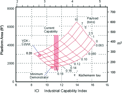
SSTO ejector ramjet/scramjet cycle solution space (Mach 12 transition)
Full size image

Figure 3.70 shows the solution map for the all-rocket configuration. The bottom scale is for ICI in English units (ft⁻¹) for I _p and I _str, and the top scale is for ICI in SI units (m⁻¹). The left scale is in English units, and the right scale is in SI units for the planform area. The vertical bar is the ICI boundary for the all-rocket topping cycle similar to the SSME (Jenkins 2001). Note that most of the design space is to the right of the ICI boundary at 9.0–9.5 ft ⁻¹, that is, beyond the current state of the art. A kerosene-fueled supersonic cruise vehicle like Concorde has a low value of τ, about 0.035. A hydrocarbon-fueled hypersonic cruise vehicle would have a larger value of τ, about 0.063.

If the designer of a SSTO chose to pattern the design after a cruise vehicle, with a low value of τ, the design would not converge, no matter what resources were expended. Note that as the payload increases, the available design space increases. One of the dilemmas of hypersonic vehicle design is as well illustrated in this figure. Using reasoning based on subsonic aircraft, a smaller aircraft should be easier to fabricate and operate than a larger one. However, for a SSTO demonstrator, that is, a demonstrator that can actually achieve orbital speed and altitude, the opposite is the case. The minimum sized, zero-payload demonstrator is on the ICI boundary and at the maximum value of τ. An operational vehicle with a 7.0 t payload as analyzed by Czysz and Vandenkerckhove (2000) has a significant reduction of the ICI value needed. As the payload increases, the τ value at the ICI boundary decreases. Then, for a 10 t payload the minimum value of τ is 0.14. Note that it would be possible to build a hypersonic demonstrator that could achieve Mach 12 for, say, just 5-min flight time, but the mass ratio for that mission might be on the order of 1.8, far from the 8.1 ratio required to reach orbital speed and altitude.

Figure 3.71 shows the solution map for the rocket plus ejector ramjet/scramjet operating as an airbreathing system to Mach 8. The bottom scale is for ICI in English units for I _p and I _str, and the top scale is for ICI in SI units. The left scale is in English units and the right scale is in SI units for the planform area. The vertical bar is the ICI boundary for the rocket plus ejector ramjet/scramjet operating as an airbreathing system to Mach 8, and it is at the 9.0–9.5 ft⁻¹ value, the same as for the all-rocket launcher. In terms of industrial capability required, this analysis points to an equality of requirements. As with the previous case, most of the design space is to the right of the ICI boundary, that is, beyond the current state of the art. Both the operational example and the demonstrator example have the same ICI value as the previous rocket case. Clearly, the Mach 8 airbreather is about equal, in terms of technical challenge, to the all-rocket vehicle.

Figure 3.72 shows the solution map for the rocket plus ejector ramjet/scramjet, this time operating as an airbreathing system to Mach 12. The bottom scale is for ICI in English units for I _p and I _str, and the top scale is for ICI in SI units. The left scale is in English units, and the right scale is in SI units for the planform area. The vertical bar is the ICI boundary for the rocket plus ejector ramjet/scramjet operating as an airbreathing system to Mach 12, and it is to the right of the previous two cases, at a value in the 11–11.5 ft ⁻¹ range. Clearly, a greater industrial capability fraction of the design space is available for converged designs, but those designs require a higher value of ICI. As with the two previous cases, most of the design space is to the right of the ICI boundary, that is, beyond the current state of the art. Both the operational example and the demonstrator example have a greater ICI value than the previous two cases.

In summary, as the value for the structural index can be assumed to be the same for all three cases presented, the Mach 8 airbreather is about equal, in terms of the technical challenge, to the all-rocket vehicle, but the Mach 12 airbreather represents a greater challenge particularly in propulsion.

It is important to note that the conventional aircraft design wisdom puts SSTO designs out of reach of current industrial capability. The SSTO challenges are similar for all-rocket and airbreather, but increasingly difficult as the Mach number, when airbreathing propulsion must transition to rocket propulsion, increases beyond Mach 8. Given the similarity of the industrial challenge, the question is: What are the differences in weight for the airbreather compared to the all-rocket vehicle? Figure 3.73 answers this key question. For approximately the same empty weight, the gross weight of the rocket vehicle is at least twice heavier compared to the combined-cycle vehicle. The shaded area indicates the area to the left of the ICI boundary in Figs. 3.70 and 3.72. Increasing the slenderness beyond τ ≈ 0.12 offers no benefit in reducing either the operational empty weight or the gross weight.

3.8.2 Transatmospheric Space Launcher: Lessons Learned

(1)
In the authors’ judgment, the real issue for space launcher organizations is not technology, but creating an operationally affordable vehicle that can be as reliable and frequent in delivering cargo to orbit as aircraft are efficient in delivering cargo to another city (Penn and Lindley 1998). The launcher that is at least partially airbreathing can meet the needs of frequent flights to orbit. This potential may still not be recognized by the space organizations, and typical of their positions is “… the only propulsion system for the 21st century is rocket …” (Freeman et al. 1995). Less frequently flying heavy lift vehicles to LEO are a different matter, and vehicles designed for eventual full reuse, such as NPO Energia, are appropriate.
(2)
Three vehicle sizing approaches of increasing generality and scope have been presented that integrate simultaneous volume and weight sizing solutions as function of configuration concept, propulsion, propulsion-aerodynamic-structural-energy efficiency, and trajectory. Methods of describing and visualizing the total parametric design space topography, and the design space where solutions are possible, have been described. The parameter interactions are such that a priori judgments often lead to non-converged results.
(3)
A broad spectrum of potential airbreathing propulsion systems have been described, and their impact on weight ratio, takeoff mode, and size are presented to show the impact of airbreathing type of propulsion.
(4)
The vehicle sizing approach described enables design to specific requirements. This provides greater physical insights into the multi-disciplinary hypersonic aircraft system interactions than do constant size exercises provide in comparison. With constant size, negative payloads can and do result. The physical interpretation of negative payload and the volume of that payload are obscure.
(5)
The key to creating an affordable, flexible, and reliable launcher is a lightweight high-thrust propulsion system. A number of different engine cycles have been discussed in this chapter. Some employ turbo machinery as part of the cycle. The need for a high specific impulse and high thrust leads to the thermally integrated LACE ejector ramjet concept. The desire to reduce onboard carried oxidizer to a minimum leads to in-flight air collection and separation adaptation of the thermally integrated LACE ejector ramjet concept. As the NASA-sponsored HyFAC study clearly showed, as good as turbojets are for fighters, the poor launcher transonic acceleration makes non-integrated gas turbine engines an expensive price to pay for familiar conventionality.
(6)
The TSTO or mobile-based SSTO with the Liquid Air Cycle Engine (LACE) incorporated into the subsonic carrier for collection purposes can already provide a flexible, fully reusable concept with only subsonic staging.
(7)
For the SSTO without in-flight collection, the use of scramjets is mandatory. To represent the SSTO as an unachievable device in the near term is to discredit the pioneers of the late 1950s and 1960s who built and successfully tested these engines up to at least Mach 8 for the inlet diffuser, the exit, and their ability to duplicate conditions. With air collection, the use of scramjets is not essential, provided advanced light-weight high-internal pressure and temperature ramjets are available. With subsequent upgrades, scramjets with increased payloads have significant growth potential.

3.9 Hypersonic Configurations: Geometric Characteristics

This section collects the fundamental sizing relationships from Hypersonic Convergence (Czysz 1986) and then develops the geometrical relationships that are inherent in the approach.

3.9.1 Configuration Continuum

The fundamental premise of the approach is that the geometry of hypersonic vehicles relates to volume and area such that it can be approached parametrically rather than via single point designs. Ten families of hypersonic configurations have been developed in the Hypersonic Convergence data-base: All configuration geometries have delta planforms with the wing apex beginning at the nose. A NASA Langley cylinder-wing configuration (WB004C) was added as a reusable all-rocket reference point.

Overall, there are two scaling modes: (A) Hold the sweep angle constant and vary the volume by changing the maximum cross-sectional area; (B) hold the cross section constant and vary the wing sweep through 72° to 80°. The configurations and the pertinent equations are included in this chapter to enable the reader to develop the desired relationships. In this discussion, the authors used a fixed sweep angle of 78° for all configurations. All the curves shown are for pointed bodies.

To begin, Hypersonic Convergence is briefly reviewed to show the derivation of the three principal size-determining elements and where the geometric characteristic of a particular configuration does play a role. The three principal elements are as follows: (1) the ratio propellant volume to planform area, (2) the ratio propellant density to weight ratio minus one, and (3) the magnitude of planform area. The geometry of the configuration will be of first-order importance (highest-of-importance) in the first and third elements. The configuration will play a role in the second element, but only as a correction to the weight ratio term for thrust-to-drag ratio. Beginning with the definition of weight ratio, we have:

$$ W_{\text{R}} = \frac{{W_{\text{TOGW}} }}{{W_{\text{OWE}} }} $$

(3.57a)

$$ W_{\text{R}} = \frac{{W_{\text{OWE}} + W_{\text{ppl}} }}{{W_{\text{OWE}} }} $$

(3.57b)

$$ W_{\text{R}} = 1 + \frac{{W_{\text{ppl}} }}{{W_{\text{OWE}} }} $$

(3.57c)

The fundamental definition of Operational Weight Empty (W _OWE) is given by:

$$ W_{\text{OWE}} = \frac{{W_{\text{ppl}} }}{{W_{\text{R}} - 1}} $$

(3.58a)

$$ W_{\text{OWE}} = \frac{{V_{\text{ppl}} }}{{S_{\text{plan}} }} \cdot \frac{{\rho_{\text{ppl}} }}{{W_{\text{R}} - 1}} \cdot S_{\text{plan}} $$

(3.58b)

$$ W_{\text{OWE}} = W_{\text{OEW}} + W_{\text{pay}} + W_{\text{crew}} $$

(3.58c)

Incorporating Küchemann’s volume parameter

$$ \tau = \frac{{V_{\text{total}} }}{{S_{\text{plan}}^{1.5} }} $$

(3.59)

we obtain

$$ W_{\text{OWE}} = \frac{{\rho_{\text{ppl}} }}{{W_{\text{R}} - 1}} \cdot \frac{{V_{\text{ppl}} }}{{V_{\text{tot}} }} \cdot \tau \cdot S_{\text{plan}}^{1.5} $$

(3.60)

Introducing the geometric parameter K _w, the ratio of wetted (surface) area to planform area, and a correlation K _str for the structure weight fraction with respect to the W _OEW, we have:

$$ K_{\text{w}} = \frac{{S_{\text{wet}} }}{{S_{\text{plan}} }} $$

(3.61)

With

$$ \frac{{W_{\text{str}} }}{{W_{\text{OEW}} }} = \frac{{K_{\text{str}} }}{{S_{\text{plan}}^{0.138} }} $$

(3.62)

and

$$ K_{\text{str}} = \frac{{W_{\text{str}} /W_{\text{OEW}} }}{{S_{\text{plan}}^{0.138} }} $$

(3.63a)

$$ K_{\text{str}} = 0.228^{ \pm 0.035} \times \tau^{0.206} $$

(3.63b)

We obtain a relationship for the technology of the airframe structure (including thermal protection) as related to the propulsion-propellant technology and geometry:

$$ \frac{{W_{\text{str}} }}{{S_{\text{wet}} }} = \left( {\frac{{\rho_{\text{ppl}} }}{{W_{\text{R}} - 1}}} \right) \cdot \left( {\frac{{V_{\text{ppl}} }}{{V_{\text{tot}} }}} \right) \cdot \frac{{\frac{{W_{\text{str}} }}{{W_{\text{OEW}} }}}}{{1 + \frac{{W_{\text{use}} }}{{W_{\text{OEW}} }}}} \cdot \frac{{\tau \cdot S_{\text{plan}}^{1.5} }}{{K_{\text{w}} }} $$

(3.64)

With respect to the propellant volume fraction, V _ppl, the correlation from a series of detailed-design hypersonic cruise vehicles, from an F-15 weight class to an AN-225 weight class, provided the data-base. Because the correlation parameter K _v in Eq. (3.65a) is dimensional, two versions are given for both unit systems. The original correlations were for an all-electronic, high-density payload. Consequently, the initial value, K _v0, is scaled with respect the bulk density of the payload. This is the payload weight divided by the payload bay volume.

$$ \frac{{V_{\text{ppl}} }}{{V_{\text{tot}} }} \approx K_{\text{v}} \cdot S_{\text{plan}}^{0.0717} {\text{ (English)}} $$

(3.65a)

$$ \frac{{V_{\text{ppl}} }}{{V_{\text{tot}} }} \approx 1.1857 \cdot K_{\text{v}} \cdot S_{\text{plan}}^{0.0717} {\text{ (Metric)}} $$

(3.65b)

We obtain for the scaled propellant volume fraction:

$$ K_{\text{v}} = K_{\text{v0}} - 6.867 \cdot 10^ {- 3}{ \cdot \tau^{ - 1} } + 8.2777 \cdot 10^ {- 4}{ \cdot \tau^{ - 2} } - 2.811 \cdot 10^ {- 5}{ \cdot \tau^{ - 3} } $$

(3.66)

with

$$ K_{\text{v0}} = 0.40 \cdot \left( {\frac{{\rho_{\text{pay}} }}{5.0}} \right)^{0.123} $$

(3.67a)

$$ K_{\text{v0}} = 0.40 \cdot \left( {\frac{{\rho_{\text{pay}} }}{176.5}} \right)^{0.123} $$

(3.67b)

The payload fraction has been correlated for two classes of vehicles. Equation 3.68a is for the propulsion integrated configuration concepts with a body-integrated inlet ramp system and exhaust nozzle. Equation 3.68b is for the blunt-base rocket powered hypersonic glider configuration concepts. Note that the payload fraction is a function of both the geometrical slenderness and the absolute value of payload. The payload must be in metric ton for Eqs. 3.68a, b.

$$ \frac{{W_{\text{pay}} }}{{W_{\text{OEW}} }} = \frac{{e^{(2.10 \cdot \tau )} }}{24.79} \cdot e^{{[0.71 \cdot \ln (W_{\text{pay}} )]}} $$

$$ \frac{{W_{\text{pay}} }}{{W_{\text{OEW}} }} = \frac{{e^{(1.29 \cdot \tau )} }}{25.4} \cdot e^{{[0.71 \cdot \,\ln (W_{\text{pay}} )]}} $$

(3.68)

Equation 3.64 can then be written as:

$$ \frac{{W_{\text{str}} }}{{S_{\text{wet}} }} = \frac{{K_{\text{str}} \cdot K_{\text{v}} \cdot \tau }}{{K_{\text{w}} }} \cdot \left( {\frac{{\rho_{\text{ppl}} }}{{W_{\text{R}} - 1}}} \right) \cdot \frac{{S_{\text{plan}}^{0.7097} }}{{1 + \frac{{W_{\text{pay}} }}{{W_{\text{OEW}} }}}} $$

(3.69)

This equation can be rearranged to yield a first-order or highest-of-importance estimate of the vehicle planform area based on the available industrial capability (technology), payload faction, and configuration geometry:

$$ S_{\text{plan}} = \left[ {\left( {\frac{{K_{\text{w}} }}{\tau }} \right) \cdot K_{\text{str}} \cdot K_{\text{v}} \cdot \frac{{\frac{{\rho_{\text{ppl}} }}{{(W_{\text{R}} - 1)}}}}{{\frac{{W_{\text{str}} }}{{S_{\text{wet}} }}}} \cdot \left( {1 + \frac{{W_{\text{pay}} }}{{W_{\text{OEW}} }}} \right)} \right]^{1.409} $$

(3.70)

The three primary terms are then:

$$ \frac{{\frac{{\rho_{\text{ppl}} }}{{(W_{\text{R}} - 1)}}}}{{\frac{{W_{\text{str}} }}{{S_{\text{wet}} }}}} = \frac{{I_{\text{p}} }}{{I_{\text{str}} }} $$

(3.71a)

$$ \left( {1 + \frac{{W_{\text{pay}} }}{{W_{\text{OEW}} }}} \right) = 1 + \frac{\exp (2.10 \cdot \tau )}{24.79} \cdot \exp [0.71 \cdot \ln (W_{\text{pay}} )] $$

(3.71b)

$$ \left( {\frac{{K_{w} }}{\tau }} \right) \cdot K_{\text{str}} \cdot K_{\text{v}} = \left( {\frac{{K_{\text{w}} }}{\tau }} \right) \cdot \frac{{0.093{ \pm 0.017} }}{{\tau^{0.794} }} $$

(3.71c)

A most likely value for K _v of 0.40 ±0.02 is assumed for the last term. For the (K _w/τ) term, ten families of hypersonic configurations from the Hypersonic Convergence data-base (Czysz 1986) are given. As introduced earlier, all configurations have delta planforms with the wing apex beginning at the nose. The NASA Langley cylinder-wing configuration (WB004C) has been added as a reusable all-rocket reference point. There are two different scaling modes. The first does fix the sweep angle and it varies the volume by changing the maximum cross-sectional area. The second does fix the cross section and it varies the wing sweep from 72° through 80°. For this report, the authors selected to fix the sweep angle at 78° for all configurations. The configurations and pertinent equations are provided here, enabling the reader to generate their own scaling models. All the curves shown in this reference are for pointed bodies. A spatula-body fixes the length and adds width and volume. Since the length determines the engine module height and length, a fixed length, but wider, vehicle can incorporate an increased number of the same engine modules into the configuration. This eases the concerns of the propulsion community with respect to engine module certification. The spatula-nosed waveriders from the University of Maryland have essentially the same characteristics as the blended-body (Mark Lewis, private communication, June 1997).

For the ten configuration families (geometry lineages) are constant 78° sweep-angle variable cross-sectional shapes. The rocket-derived propulsion includes LACE and deeply cooled rocket cycles. Airbreathing-derived propulsion-integrated hypersonic configurations are: (1) blended-body, (2) wing-body (not cylinder-wing), and (3) Nonweiler waverider. Rocket-derived hypersonic gliders are: (4) diamond cross section, base height to width 0.1–1.0; (5) elliptical cross section, base height to width from 0.1 to 1.0; (6) trapezoidal cross section, base top width to bottom width from 0 to 1.0; (7) blunted right-circular cone, nose-to-base diameter ratio from 0 to 0.3; (8) half-diamond cross section, base height to width from 0.05 to 0.5; (9) half-elliptical cross section, base height to width from 0.05 to 0.5; and (10) half-blunted right-circular cone, nose-to-base diameter ratio from 0 to 0.3. The eleventh configuration (11) is the NASA Langley cylinder-wing (WB004C) configuration (Martinovic and Cerro 2002), which is used as a vertical launch and recoverable rocket vehicle reference. The exposed wing area and diameter of the tank have been held constant. The volume changes by varying the length-to-diameter of the cylinder. This configuration has not been used in this book.

Figure 3.74 shows the wetted area to planform area ratio, K _w = S _wet/S _plan, versus τ for configurations that include aerodynamic control as surfaces as shown in Figs. 3.42 and 3.48. These are possible candidates for space launchers having values of τ less than 0.20 and lower values of wetted area to planform area ratio, S _wet/S _plan. The wing-body and Nonweiler waverider have larger values of wetted area to planform area ratio than integral wing-body configurations. The WB004C configuration has very different geometric properties compared to the highly swept integral wing-body configurations. It is essentially a constant τ configuration (0.162–0.167) over a 2 to 1 volume ratio, which means that volume changes require planform area changes. The full range of hypersonic shapes extend beyond τ = 0.20. Figure 3.75 shows a broader range of configuration characteristics up to τ = 0.50 that encompasses most hypersonic cruise aircraft, hypersonic accelerators or space launchers, and hypersonic gliders. That represents about the limit for a reasonable lift-to-drag ratio for an acceptable cross-range and down-range. Not shown is the sphere with a τ = 0.752 and a K _w = 4.00.

The elliptical cone spans the widest range of τ and K _w as it progresses from an ellipse with a height 10% of its width to a circle. The diamond and trapezoidal shapes span similar ranges. There are two trapezoidal shapes. The first one with (b/a) = 1 has a height equal to the half width. The second one with (b/a) = 2 has a height equal to the width. The parameter in the sizing equation is the ratio of τ/K _w. That ratio is plotted in Fig. 3.76 for all of the configurations shown in Fig. 3.75. The result is the collapse of the geometric characteristics into nearly a single line, see Fig. 3.76. In this graph, the sphere is shown, and it has the lowest value of the (K _w/τ) term. Clearly, the sphere has the lowest W _OEW and the highest drag, making it a simple ballistic vehicle.

The different classes of vehicles and the propellants can be differentiated on Fig. 3.76. The denser the propellant, the smaller the propellant volume and the more slender the shape and the larger the planform area with respect to the propellant volume. The important conclusion is that as a first-order estimate, only τ needs be known. After the first order estimate, then the refinement of the estimate using different geometries can proceed. The primary determinant then is the propulsion index that results from a trajectory or cruise performance analysis. The remainder of this chapter gives the configuration concepts and the description of the geometric properties.

3.9.2 Configuration Geometry Properties

There are a wide variety of configurations possible for reusable spacecraft. But if the requirements for a transportation system to space and back are to be met, the configuration spectrum is significantly narrowed. Two basic configuration types have been employed in the US.

One is for all-rocket and airbreathing rocket-cycle propulsion that can operate as airbreathing propulsion to about Mach 6, see upper left in Fig. 3.77. For the rocket propulsion and airbreathing rocket propulsion concepts, a versatile variable capture, inward turning inlet (DuPont 1999) can be integrated into the vehicle configuration derived from the FDL series of hypersonic gliders developed by the Flight Dynamics Laboratory and the work of the McDonnell Douglas Astronautics Company. Because of the mass ratio to orbit, these configurations are generally VTHL vehicles.

The other configuration lineage is for airbreathing propulsion systems that require a propulsion-configured vehicle, where the entire underside of the vehicle is an integrated propulsion system, see lower right in Fig. 3.77. The thermally integrated airbreathing combined-cycle configuration concept is derived from the McDonnell Douglas (St. Louis) Advanced Design organization. This is the family of hypersonic, rocket accelerated, and airbreathing cruise vehicles (Pirrello and Czysz 1970). Depending on mass ratio, these vehicles can takeoff horizontally (HTHL) or be launched vertically (VTHL) and always land horizontally. The vehicle concept initially conceived in the 1960s was an airbreathing, propulsion-configured vehicle accelerated by a main rocket in the aft end of the body. Today, such basic configuration can still retain this strategy or use a RBCC propulsion concept. Overall, both basic shapes are functions of τ, that is, for a given planform area, the cross-sectional distribution is determined by the volume required.

The following addresses configurations that are designed to be controlled in the entry glide and for airbreathers, and for the other class of vehicles to be controlled on the exit and entrance flight path. The first part deals with configurations specifically designed to integrate airbreathing systems and the second with hypersonic glider configurations.

Airbreathing Configuration Concepts. The section at the end of this chapter provides equations that give the geometric characteristics of airbreathing configurations. The airbreathing hypersonic vehicle is not just an aerodynamic shape with an engine attached, but indeed the compression side of the vehicle is the inlet, combustor and nozzle. At Mach 6, an isolated nacelle is almost as long as the airframe. A conventional freestream inlet, that is, one designed to operate at the freestream Mach number, is very difficult to control at hypersonic Mach numbers. Using the air vehicle as the propulsion system means that the engine inlet Mach number is considerably less than flight speed, and more amenable to stability and control. For the family of hypersonic vehicles shown in Fig. 3.78, the compression side is identical for all the blended-body configurations. In fact, to have the wing-body operate efficiently, it must have essentially the same underside as the blended-body. The Nonweiler waverider is a special case due to its conical flow field. There is the same number of ramps, but they are designed three-dimensionally to create a family of converging conical shocks.

General Hypersonic Glider Configuration Concepts. These vehicles have blunt bases and are appropriate for rocket-powered hypersonic gliders, such as the FDL-7 series. These configurations have been the basis of many hypersonic gliders by the US Air Force and others with an interest in significant cross-range and down-range over the past 50 years. These vehicles are very different from wing-body configuration concepts such as the Space Shuttle Orbiter, X-37 and XS-1 (first stage), or all-body (lifting body) configuration concepts like the X-24A, M2-F3, HL-10, Dream Chaser, and X-38, since they have substantially better performance with reduced entry heat load. It is possible to use some of the FDL-lineage configuration concepts, such as deeply cooled and LACE propulsion concepts that are limited to Mach numbers less than 6. The key to a successful airbreathing concept is the maintenance of sharp leading edges, in that they reduce drag and thus entropy production during flight. For more detail, see Czysz (1986).

The remaining figures in this section show the hypersonic glider and airbreathing cruiser/accelerator geometric characteristics of configuration concepts and list related equations.

RIGHT-CIRCULAR POINTED CONE

$$ A_{\text{base}} = \pi \cdot r^{2} $$

(3.72a)

$$ S_{\text{plan}} = r^{2} \cdot \,\tan \varLambda $$

(3.72b)

$$ S_{\text{wet}} = \pi \cdot r^{2} \cdot \left( {1 + \frac{1}{\cos \varLambda }} \right) $$

(3.72c)

$$ V_{\text{tot}} = \frac{{\pi \cdot r^{3} }}{3} \cdot \tan \varLambda $$

(3.72d)

$$ K_{\text{w}} = \pi \cdot \left( {\frac{1}{\tan \varLambda } + \frac{1}{\sin \varLambda }} \right) $$

(3.72e)

$$ \tau = \frac{\pi }{{3 \cdot \sqrt {\tan \varLambda } }} $$

(3.72f)

$$ \tan \varLambda = \frac{\pi }{3 \cdot \tau } $$

(3.72g)

$$ \tau_{{78^{ \circ } }} = 0.4826 $$

(3.72h)

$$ (K_{\text{w}} )_{78^\circ } = 4.160 $$

(3.72i)

$$ 0.54 \le \tau \le 0.39 $$

(3.72j)

BLUNTED CONE

$$ A_{\text{base}} = \frac{{\tau \cdot r_{\text{b}}^{2} }}{2} $$

(3.73a)

$$ S_{\text{plan}} = r_{\text{b}}^{2} \cdot \,\tan\Lambda \cdot \left[ {1 + \left( {\frac{{r_{\text{n}} }}{{r_{\text{b}} }}} \right)^{2} } \right] + \frac{{\pi \cdot r_{\text{b}}^{2} }}{2} \cdot \left( {\frac{{r_{\text{n}} }}{{r_{\text{b}} }}} \right)^{2} $$

(3.73b)

$$ S_{\text{wet}} = \pi \cdot r_{\text{b}}^{2} \cdot \left[ {1 + \frac{{1 + \left( {\frac{{r_{\text{n}} }}{{r_{\text{b}} }}} \right)^{2} }}{\cos \varLambda } + 2 \cdot \left( {\frac{{r_{\text{n}} }}{{r_{\text{b}} }}} \right)^{2} } \right] $$

(3.73c)

$$ V_{\text{tot}} = \frac{{\pi \cdot r_{\text{b}}^{3} }}{3} \cdot \left( {1 - \frac{{r_{\text{n}} }}{{r_{\text{b}} }}} \right) \cdot \left[ {1 + \frac{{r_{\text{n}} }}{{r_{\text{b}} }} + \left( {\frac{{r_{\text{n}} }}{{r_{\text{b}} }}} \right)^{2} } \right] \cdot \tan \varLambda + \frac{{\pi \cdot r_{\text{b}}^{3} }}{2} \cdot \left( {\frac{{r_{\text{n}} }}{{r_{\text{b}} }}} \right)^{3} $$

(3.73d)

$$ (K_{\text{w}} )_{78^\circ } = 4.600 \cdot \left( {\frac{{r_{\text{n}} }}{{r_{\text{b}} }}} \right)^{2} - 2.350 \cdot \frac{{r_{\text{n}} }}{{r_{\text{b}} }} + 4.111 $$

(3.73e)

$$ \tau_{78^\circ } = 0.3048 \cdot \left( {\frac{{r_{\text{n}} }}{{r_{\text{b}} }}} \right)^{2} + 0.01875 \cdot \frac{{r_{\text{n}} }}{{r_{\text{b}} }} + 0.04826 $$

(3.73f)

$$ 0.00 \le \frac{{r_{\text{n}} }}{{r_{\text{b}} }} \le 0.30 $$

(3.73g)

$$ 0.4826 \le \tau \le 0.52 $$

(3.73h)

ELLIPSE

$$ A_{\text{base}} = \pi \cdot a^{2} \cdot e $$

(3.74a)

$$ S_{\text{plan}} = a^{2} \cdot \tan \varLambda $$

(3.74b)

$$ S_{\text{wet}} = \pi \cdot a^{2} \cdot \frac{(1 + e)}{\cos \varLambda } \cdot \left( {1 + \frac{{R^{2} }}{4} + \frac{{R^{4} }}{64} + \frac{{R^{6} }}{256}} \right) + \pi \cdot a^{2} \cdot e $$

(3.74c)

$$ V_{\text{tot}} = \frac{{\pi \cdot a^{3} \cdot e}}{3} \cdot \,\tan \varLambda $$

(3.74d)

$$ (K_{\text{w}} )_{78^\circ } = 2.404 \cdot \tau^{2} + 2.920 \cdot \tau + 2.174 $$

(3.74e)

$$ \tau_{78^\circ } = 0.4826 \cdot \frac{b}{a} $$

(3.74f)

$$ 0.01 \le \frac{a}{b} \le 1.0 $$

(3.74g)

$$ 0.0483 \le \tau \le 0.4826 $$

(3.74h)

$$ e = \frac{b}{a} $$

(3.74i)

$$ R = \frac{1 - e}{1 + e} $$

(3.74j)

DIAMOND

$$ A_{\text{base}} = 2 \cdot a^{2} \cdot e $$

(3.75a)

$$ S_{\text{plan}} = a^{2} \cdot \,\tan \varLambda $$

(3.75b)

$$ S_{\text{wet}} = 2 \cdot a^{2} \cdot \sqrt {1 + e^{2} } \cdot \,\tan \varLambda + 2 \cdot a^{2} \cdot e $$

(3.75c)

$$ V_{\text{tot}} = \frac{{2 \cdot a^{3} \cdot e}}{3} \cdot \,\tan \varLambda $$

(3.75d)

$$ (K_{\text{w}} )_{78^\circ } = 8.023 \cdot \tau^{2} + 1.872 \cdot \tau + 2.173 $$

(3.75e)

$$ \tau_{78^\circ } = 0.3074 \cdot \frac{b}{a} $$

(3.75f)

$$ 0.01 \le \frac{a}{b} \le 1.0 $$

(3.75g)

$$ 0.0307 \le \tau \le 0.307 $$

(3.75h)

$$ e = \frac{b}{a} $$

(3.75i)

TRAPEZOID

$$ A_{\text{base}} = a^{2} \cdot e \cdot (1 + x) $$

(3.76a)

$$ S_{\text{plan}} = a^{2} \cdot \,\tan \varLambda $$

(3.76b)

$$ S_{\text{wet}} = a^{2} \cdot \left[ {(1 + x) + \frac{{\sqrt {e^{2} + (1 + x)^{2} } }}{\cos \varLambda }} \right] $$

(3.76c)

$$ V_{\text{tot}} = \frac{{a^{3} \cdot (1 + x) \cdot e}}{3} \cdot \,\tan \varLambda $$

(3.76d)

$$ (K_{\text{w}} )_{78^\circ } = 2.906 - 2.022 \cdot \tau + 15.706 \cdot \tau^{2} $$

(3.76e1)

$$ \tau_{78^\circ } = 0.1535 \cdot x + 0.1538 $$

(3.76e2)

$$ b/a = 1.0 $$

(3.76e3)

$$ (K_{\text{w}} )_{{78{^\circ }}} = 3.013 + 0.706 \cdot \tau + 5.438 \cdot \tau^{2} $$

(3.76f1)

$$ \tau_{{78{^\circ }}} = 0.2300 \cdot x + 0.2310 $$

(3.76f2)

$$ b/a = 1.5 $$

(3.76f3)

$$ (K_{\text{w}} )_{{78{^\circ }}} = 3.093 + 1.064 \cdot \tau + 3.093 \cdot \tau^{2} $$

(3.76g1)

$$ \tau_{{78{^\circ }}} = 0.3075 \cdot x + 0.3075 $$

(3.76g2)

$$ b/a = 2.0 $$

(3.76g3)

$$ 0.0 \le x \le 1.0\left( {{\text{from}}\,{\text{triangle}}\,{\text{to}}\,{\text{square}}\,{\text{base}}} \right) $$

(3.76h)

$$ 0.154 \le \tau \le 0.615 $$

(3.76i)

$$ e = b/a $$

(3.76j)

$$ x = {\text{top}}\,{\text{width/bottom}}\,{\text{width}} $$

(3.76k)

POINTED HALF-CONE

$$ A_{\text{base}} = \frac{{\pi \cdot r^{2} }}{2} $$

(3.77a)

$$ S_{\text{plan}} = r^{2} \cdot \,\tan \varLambda $$

(3.77b)

$$ S_{\text{wet}} = \frac{{\pi \cdot r^{2} }}{2} \cdot \left( {1 + \frac{1}{\cos \varLambda }} \right) + r^{2} \cdot \,\tan \varLambda $$

(3.77c)

$$ V_{\text{tot}} = \frac{{\pi \cdot r^{3} }}{6} \cdot \,\tan \varLambda $$

(3.77d)

$$ K_{\text{w}} = \frac{\pi }{2} \cdot \left( {\frac{1}{\tan \varLambda } + \frac{1}{\sin \varLambda }} \right) + 1 $$

(3.77e)

$$ \tau = \frac{\pi }{{6 \cdot \sqrt {\tan \varLambda } }} $$

(3.77f)

$$ \tan \varLambda = \frac{\pi }{6 \cdot \tau } $$

(3.77g)

$$ 0.0307 \le \tau \le 0.307 $$

(3.77h)

$$ (K_{\text{w}} )_{78^\circ } = 3.220 $$

(3.77i)

$$ \tau_{{78{^\circ }}} = 0.241 $$

(3.77j)

BLUNTED HALF-CONE

$$ A_{\text{base}} = \frac{{\pi \cdot r_{\text{b}}^{2} }}{4} $$

(3.78a)

$$ S_{\text{plan}} = r_{\text{b}}^{2} \cdot \tan \varLambda \cdot \left[ {1 - \left( {\frac{{r_{\text{n}} }}{{r_{\text{b}} }}} \right)^{2} } \right] + \frac{{\pi \cdot r_{\text{b}}^{2} }}{2} \cdot \left( {\frac{{r_{\text{n}} }}{{r_{\text{b}} }}} \right)^{2} $$

(3.78b)

$$ S_{\text{wet}} = \frac{{\pi \cdot r_{\text{b}}^{2} }}{2} \cdot \left[ {1 + \frac{{1 + \left( {\frac{{r_{\text{n}} }}{{r_{\text{b}} }}} \right)^{2} }}{\cos \varLambda } + 2 \cdot \left( {\frac{{r_{\text{n}} }}{{r_{\text{b}} }}} \right)^{2} } \right] + S_{\text{plan}} $$

(3.78c)

$$ V_{\text{tot}} = \frac{{\pi \cdot r_{\text{b}}^{3} }}{6} \cdot \left[ {\left( {1 - \frac{{r_{\text{n}} }}{{r_{\text{b}} }}} \right) \cdot \left[ {1 + \frac{{r_{\text{n}} }}{{r_{\text{b}} }} + \left( {\frac{{r_{\text{n}} }}{{r_{\text{b}} }}} \right)^{2} } \right] \cdot \tan \varLambda + 2 \cdot \left( {\frac{{r_{\text{n}} }}{{r_{\text{b}} }}} \right)^{3} } \right] $$

(3.78d)

$$ (K_{\text{w}} )_{78^\circ } = 58.592 \cdot \left( {\frac{{r_{\text{n}} }}{{r_{\text{b}} }}} \right)^{2} - 25.755 \cdot \frac{{r_{\text{n}} }}{{r_{\text{b}} }} + 5.970 $$

(3.78e)

$$ \tau_{78^\circ } = 0.1381 \cdot \left( {\frac{{r_{\text{n}} }}{{r_{\text{b}} }}} \right)^{2} + 0.01643 \cdot \frac{{r_{\text{n}} }}{{r_{\text{b}} }} + 0.2409 $$

(3.78f)

$$ 0.2409 \le \tau \le 0.258 $$

(3.78g)

HALF-ELLIPSE

$$ A_{\text{base}} = \pi \cdot a^{2} \cdot \frac{e}{2} $$

(3.79a)

$$ S_{\text{plan}} = a^{2} \cdot \tan \varLambda $$

(3.79b)

$$ S_{\text{wet}} = \frac{{\pi \cdot a^{2} }}{2} \cdot \left[ {\frac{{\left( {1 + e} \right)}}{\cos \varLambda } \cdot \left( {1 + \frac{{R^{2} }}{4} + \frac{{R^{4} }}{64} + \frac{{R^{6} }}{256}} \right) + e} \right] + S_{\text{plan}} $$

(3.79c)

$$ V_{\text{tot}} = \frac{{\pi \cdot a^{3} \cdot e}}{6} \cdot \tan \varLambda $$

(3.79d)

$$ (K_{\text{w}} )_{78^\circ } = 2.226 + 2.917 \cdot \frac{b}{a} + 4.689 \cdot \left( {\frac{b}{a}} \right)^{2} $$

(3.79e)

$$ \tau_{78^\circ } = 0.2413 \cdot \frac{b}{a} $$

(3.79f)

$$ 0.0241 \le \tau \le 0.241 $$

(3.79g)

$$ e = \frac{b}{a} $$

(3.79h)

$$ R = \frac{1 - e}{1 + e} $$

(3.79h)

HALF-DIAMOND

$$ A_{\text{base}} = a^{2} \cdot e $$

(3.80a)

$$ S_{\text{plan}} = a^{2} \cdot \tan \varLambda $$

(3.80b)

$$ S_{\text{wet}} = a^{2} \cdot [\sqrt {1 + e^{2} } \cdot \tan \varLambda + e] + S_{\text{plan}} $$

(3.80c)

$$ V_{\text{tot}} = \frac{{a^{3} \cdot e}}{6} \cdot \tan \varLambda $$

(3.80d)

$$ (K_{\text{w}} )_{78^\circ } = 2.228 + 1.865 \cdot \tau + 15.387 \cdot \tau^{2} $$

(3.80e)

$$ \tau_{78^\circ } = 0.154 \cdot \frac{b}{a} $$

(3.80f)

$$ 0.0154 \le \tau \le 0.154 $$

(3.80g)

$$ e = \frac{b}{a} $$

(3.80h)

TRUNCATED DOUBLE CONE (circa 1965)

$$ A_{\hbox{max} } = \pi \cdot r^{2} $$

(3.81a)

$$ S_{\text{plan}} = r^{2} \cdot \tan \varLambda \cdot \left[ {1 + \left[ {1 - \left( {\frac{{r_{\text{b}} }}{r}} \right)^{2} } \right] \cdot \frac{\tan \varLambda }{\tan (\varLambda - 3)}} \right] $$

(3.81b)

$$ S_{\text{wet}} = \pi \cdot r^{2} \cdot \left[ {\frac{1}{\cos \varLambda } + \frac{{1 - \left( {\frac{{r_{\text{b}} }}{r}} \right)^{2} }}{\cos (\varLambda - 3)} + \left( {\frac{{r_{\text{b}} }}{r}} \right)^{2} } \right] $$

(3.81c)

$$ V_{\text{tot}} = \frac{{\pi \cdot r^{3} }}{3} \cdot \left[ {\tan \varLambda + \left[ {1 - \left( {\frac{{r_{\text{b}} }}{r}} \right)^{3} } \right] \cdot \tan (\varLambda - 3)} \right] $$

(3.81d)

$$ (K_{\text{w}} )_{78^\circ } = 3.622 $$

(3.81e)

$$ \tau_{78^\circ } = 0.383 $$

(3.81f)

WING-CYLINDER (NASA Langley WB004C)

$$ A_{\text{base}} = \left[ {\frac{\pi }{4} \cdot D^{2} + 0.35 \cdot D^{2} } \right] \cdot 0.4444 $$

(3.82a)

$$ S_{\text{plan}} = \left[ {3.375 \cdot D^{2} + \left( {\frac{L}{D}} \right) \cdot D^{2} + \frac{\pi }{4} \cdot N \cdot D^{2} } \right] \cdot 0.4444 $$

(3.82b)

$$ S_{\text{wet}} = \left[ \begin{aligned} & 7.12 \cdot D^{2} + \pi \cdot \left( {\frac{L}{D}} \right) \cdot D^{2} + \frac{{\pi \cdot D^{2} }}{4} + \\ & \frac{{\pi \cdot N \cdot D^{2} }}{4} \cdot \frac{ASIN(e)}{e} \\ \end{aligned} \right] \cdot 0.4444 $$

(3.82c)

$$ V_{\text{tot}} = 0.27 \cdot D^{3} + \frac{{\pi \cdot D^{3} }}{4} \cdot \left( {\frac{L}{D}} \right) + \frac{{\pi \cdot N \cdot D^{3} }}{6} $$

(3.82d)

$$ \tau_{1} = 0.1982 - 9.524E - 5 \cdot \left( {\frac{L}{D}} \right)_{\text{tank}} - 2.381E - 4 \cdot \left( {\frac{L}{D}} \right)_{\text{tank}}^{2} $$

(3.82e)

$$ (K_{\text{w}} )_{1} = 2.193 + 0.128 \cdot \left( {\frac{L}{D}} \right)_{\text{tank}} - 0.007524 \cdot \left( {\frac{L}{D}} \right)_{\text{tank}}^{2} $$

(3.82f)

$$ (K_{\text{v}} )_{1} = - 0.2421 + 0.2109 \cdot \left( {\frac{L}{D}} \right)_{\text{tank}} - 0.01438 \cdot \left( {\frac{L}{D}} \right)_{\text{tank}}^{2} $$

(3.82g)

$$ \tau_{2} = 0.1899 + 4.286E - 4 \cdot \left( {\frac{L}{D}} \right)_{\text{tank}} - 2.381E - 4 \cdot \left( {\frac{L}{D}} \right)_{\text{tank}}^{2} $$

(3.82h)

$$ (K_{\text{w}} )_{2} = 2.432 + 0.08833 \cdot \left( {\frac{L}{D}} \right)_{\text{tank}} - 0.00438 \cdot \left( {\frac{L}{D}} \right)_{\text{tank}}^{2} $$

(3.82i)

$$ (K_{\text{v}} )_{2} = - 0.07164 + 0.1625 \cdot \left( {\frac{L}{D}} \right)_{\text{tank}} - 0.09571 \cdot \left( {\frac{L}{D}} \right)_{\text{tank}}^{2} $$

(3.82j)

$$ 4 \le (L/D)_{\text{tank}} \le 8 $$

(3.82k)

$$ 0.186 \le \tau \le 0.193\quad N = 1 $$

(3.82l)

$$ 0.184 \le \tau \le 0.189\quad N = 2 $$

(3.82m)

$$ e = \frac{{\sqrt {2 \cdot N - 1} }}{N}{\text{nose}}\,{\text{length}} = N \cdot D $$

(3.82n)

BLENDED-BODY [BB] (McDonnell Douglas circa 1965)

$$ K_{\text{w}} = - 62.217 \cdot \tau^{3} + 29.904 \cdot \tau^{2} - 1.581 \cdot \tau + 2.469 $$

(3.83)

WING-BODY [WB]

$$ K_{\text{w}} = - 93.831 \cdot \tau^{3} + 58.920 \cdot \tau^{2} - 5.648 \cdot \tau + 2.821 $$

(3.84)

NONWEILER WAVERIDER or ALL-BODY [AB] (circa 1960)

$$ K_{\text{w}} = - 533.451 \cdot \tau^{3} + 220.302 \cdot \tau^{2} - 22.167 \cdot \tau + 3.425 $$

(3.85)

Bibliography

Ahern, J.E. (1992) “Thermal Management of Air-Breathing Propulsion Systems”, AIAA Paper 92-0514, presented at the 30th Aerospace Sciences Meeting, Reno, Nevada, January 1992.
Google Scholar
Altis, H.D. (1967) “Hypersonic Scramjet Vehicle Study”, Volume VII, Structures and Weights, MAC Report F666, McDonnell Aircraft Company, McDonnell Douglas Corporation, October 1967.
Google Scholar
Ambrose, S. (2000) Nothing Like It in the World, 1st Edition, Simon & Schuster, New York, November 2001.
Google Scholar
Anon. (1965a) “GE5/JZ6 Study, Wrap-Around Turboramjet, Turbo-Accelerator Propulsion System Study Data”, Report SS-65-2, General Electric, December 1965 (confidential).
Google Scholar
Anon. (1965b) “Structural Weight Estimation”, Vol. 1, McAIR Report 747, circa 1965.
Google Scholar
Anon. (1966a) “Hypersonic Ramjet Propulsion Program, Engine Performance”, Marquardt Report 6112, The Marquardt Corporation, August 1966 (confidential).
Google Scholar
Anon. (1966b) “MA188-XAB Baseline Dual Mode Scramjet for the McDonnell/Douglas Reusable Launch Vehicle Application”, Marquardt Letter to McAIR, 1966 (confidential).
Google Scholar
Anon. (1967) “A Study of Advanced Airbreathing Launch Vehicles with Cruise Capability”, Lockheed Report IR 21042, The Lockheed Aircraft Corporation, 1967.
Google Scholar
Anon. (1969a) “Comparative Propulsion Systems Concepts Study”, U.S. Air Force Report AFRPS-TR-69-19, September 1969 (secret).
Google Scholar
Anon. (1969b) “Variable Cycle Turboramjet GE14/JZ8”, Preliminary Performance and Installation Manual, General Electric Report., U.S. Air Force Contract AF33615-69-1245, 1969 (confidential).
Google Scholar
Anon. (1970) “Mission Requirements of Lifting Systems, Summary of Significant Results and Figures”, McDonnell Aircraft Report B947 prepared under NASA NAS 9-3562, August 1965. (Declassified 1970.)
Google Scholar
Anon. (1985) “Single-Stage-to-Orbit Concept Comparison’, Aerospace Corporation Report 86-2602-301-ADA, October 1985.
Google Scholar
Anon. (1988) “Hyperplane”, 39th International Astronautical Federation Congress, Bangalore, India, October 1988.
Google Scholar
Anon. (2015) “Declassified Manned Orbiting Laboratory (MOL) Records”, National Reconnaissance Office, October 2015.
Google Scholar
Augenstein, B.W. and Harris, E.D. (1993) “The National Aerospace Plane (NASP): Development Issues for the Follow-on Vehicle – Executive Summary”, R-3878/1-AF, A Project Air Force Report, RAND, 1993, ISBN: 0-8330-1342-4.
Google Scholar
Balepin, V.V. and Hendrick, P. (1998) “Application of the KLIN Cycle to Vertical Take-Off Lifting Body Launcher”, AIAA Paper 98-1503, presented at the 8th AIAA International Space Planes and hypersonic Systems and Technologies Conference, Norfolk, VA, 27-30 April 1998.
Google Scholar
Balepin, V.V., Dulepov, N., Folomeev, E., Harchevnikova, G., et al. (1993) “Flight Liquid Oxygen Plants for Aerospace Plane: Thermodynamic and Integration Aspects”, SAE Technical Paper 931452, Society of Automotive Engineers, April 1993.
Google Scholar
Balepin, V.V., Maita, M., Tanatsugu, N., and Murthy, S.N.B. (1996) “Deep-Cooled Turbojet Augmentation with Oxygen (Cryojet) for a SSTO Launch Vehicle”, AIAA Paper 96-3036, presented at the 32nd Joint AIAA, ASME, SAE and ASEE Propulsion Conference and Exhibit, Lake Buena Vista, FL, 1–3 July 1996.
Google Scholar
Billig, F.S. (1989) “Hypersonic Vehicles II”, Proceedings of the Short Course of Engine Airframe Integration, School of Mechanical Engineering, Purdue University, July 1989.
Google Scholar
Billig, F.S. (1991) “Propulsion Systems from Take-Off to High-Speed Flight”, in: High-Speed Flight Propulsion Systems, edited by S.N.B. Murthy and E.T. Curran, Progress in Astronautics and Aeronautics, Vol. 137, AIAA, Reston VA, 1991, pp. 21–100.
Google Scholar
Billig, F. S. (1993) “The Integration of the Rocket with a Ram-Scramjet as a Viable Transatmospheric Accelerator”, AIAA Paper 93-7017. Also in Proceedings of the 11th ISABE, International Symposium on Air Breathing Engines, Vol. 1, Tokyo, Japan, 20–24 September 1993, pp. 173–187.
Google Scholar
Billig, F.S. and Van Wie, D.M. (1987) “Efficiency Parameters for Inlets Operating at Hypersonic Speeds”, Proceedings of the 8th International Symposium on Airbreathing Engines (ISABE), Cincinnati, OH, June 1987, pp. 118–130.
Google Scholar
Camberos, J.A. and Moorhouse, D.J. (editors) (2011) Exergy Analysis and Design Optimization for Aerospace Vehicles and Systems, Progress in Astronautics and Aeronautics, Volume 238, Published by AIAA, Reston, Virginia, 2011.
Google Scholar
Chudoba, B. (2001) “Aircraft Configuration Characterisation for Project Flight Mechanics”, Issue 1, CoA Report NFP0106, College of Aeronautics, Cranfield University, April 2001.
Google Scholar
Chudoba, B. (2002) Stability and Control of Conventional and Unconventional Aircraft Configurations – A Generic Approach, First Edition, Books on Demand GmbH, January 2002. (ISBN 3-8311-2982-7).
Google Scholar
Chudoba, B. (2012) “A 21st Century Decision Aid; Aeronautics & Space Transportation Technology data-base”, Final Contract Presentation, Hypersonics Research Directorate, National Institute of Aerospace (NIA), NASA LaRC, Hampton, VA, September 2012.
Google Scholar
Chudoba, B. and Gonzalez, L. (2011) “A 21st Century Decision Aid; Aeronautics & Space Transportation Technology data-base; 2008 – Present International Hypersonic Projects”, Final Contract Presentation, Hypersonics Research Directorate, National Institute of Aerospace (NIA), NASA LaRC, Hampton, VA, 12 October 2011.
Google Scholar
Chudoba, B. and Heinze, W. (2010) “Evolution of Generic Flight Vehicle Design Synthesis”, The Aeronautical Journal, Vol. 114, No. 1159, September 2010.
Google Scholar
Chudoba, B. Coleman, G., Oza, A., Gonzalez, L., Haney, E., Ricketts, V. and Czysz, P. (2011) “Manned GEO Servicing (MGS) Crew Return Vehicle Sizing,” Final Contract Report, National Institute of Aerospace (NIA), NASA LaRC and DARPA, Section in Final Report “Manned Geosynchronous Earth Orbit (GEO) Servicing (MGS) Joint NASA/DARPA Study”, NASA SP-2012-598, MGS Study Team, NASA Headquarters and DARPA Tactical Technology Office, Washington, DC, 27 April 2011.
Google Scholar
Chudoba, B., Coleman, G., Oza, A., Gonzalez, A. and Czysz, P. (2012) “Solution-Space Screening of a Hypersonic Endurance Demonstrator”, NASA CR-2012-217774, August 2012.
Google Scholar
Chudoba, B., Haney, E., Gonzalez, L., Omoragbon, A., and Oza, A. (2015a) “Strategic Forecasting in Uncertain Environments: Hypersonic Cruise Vehicle Research & Development Case Study”, The Aeronautical Journal, Vol. 119, No. 1211, January 2015.
Google Scholar
Chudoba, B., Oza, A., Gonzalez, L. and Omoragbon, A. (2015b) “Custom Decision-Support Solutions for Aerospace Systems Development”, AVD Services LLC Dossier, November 2015.
Google Scholar
Coleman, G.J. (2008) “Hypersonic Convergence Methodology and Example”, AVD-Aero-001-2008, AVD Laboratory, Mechanical and Aerospace Department, The University of Texas at Arlington, April 2008.
Google Scholar
Coleman, G.J. (2010) “Aircraft Conceptual Design – An Adaptable Parametric Sizing Methodology,” Ph.D. Dissertation, The University of Texas at Arlington, Arlington, Texas, May 2010.
Google Scholar
Collingbourne, J.R. and Peckham, D.H. (1967) “The Lift and Drag Characteristics of Caret Wings at Mach numbers between 5 and 10” C.P. No. 930, Aeronautical Research Council, February 1966.
Google Scholar
Curran, E.T. (1993) “The Potential and Practicality of High Speed Combined Cycle Engines”, Hypersonic Combined Cycle Propulsion, AGARD Conference Proceeding No. 479, AGARD, Neuilly-Sur-Seine, France, 1993, pp. Kl-9.
Google Scholar
Czysz, P.A. (1986) “Hypersonic Convergence – High-Speed Aircraft Aero-Propulsion-Structure Systems Integration – Integrated Systems Approach to Identifying Solution Space”, Volumes I-III, Course AE-P-452-50, 1992-93, Aerospace and Mechanical Engineering Department, Parks College, Saint Louis University, 1st Edition 1986.
Google Scholar
Czysz, P.A. (1991) “Delta Clipper Sizing Program”, unpublished work, McDonnell Douglas Astronautics Co., Huntington Beach, CA, May 1991.
Google Scholar
Czysz, P.A. (1992) “Space Transportation Systems Requirements Derived from the Propulsion Performance”, Paper IAF-92-0858, presented at the 43rd International Astronautical Federation Congress, Washington, DC, September 1992.
Google Scholar
Czysz, P.A. (1993) “Rocket Based Combined Cycle (RBCC) Propulsion Systems Offer Additional Options”, 11th International Symposium on Airbreathing Engines (ISABE), Vol. 1, Tokyo, Japan, 20–24 September 1993, pp. 119–137.
Google Scholar
Czysz, P.A. (1995) “Interaction of Propulsion Performance with the Available Design Space”, Proceedings of the XII International Symposium on Airbreathing Engines (ISABE), Melbourne, Australia, September 1995.
Google Scholar
Czysz, P.A. (1996) “Propulsion Concepts and Technology Approaches that Enable a Launcher for the XXI Century”, Proceeding of the 5th International Symposium, La Propulsion dans les Transports Spatiaux, 1996, p. 15.7.
Google Scholar
Czysz, P.A. (1998) “Advanced Propulsion Concepts for the XXI Century”, International Academy of Astronautics Workshop on Advanced Propulsion Concepts, The Aerospace Corporation, El Segundo, CA, January 1998.
Google Scholar
Czysz, P.A. (2004) “Hypersonic Convergence”, AFRL-VA-WP-TR-2004-3114, Volume 1 out of 3 Volumes, Wright-Patterson Air Force Base, December 2004.
Google Scholar
Czysz, P.A. and Froning, H.D. (1995) “A Propulsion Technology Challenge - Abortable, Continuous Use Vehicles”, Paper IAF-95-S.2.03, presented at the 46th International Astronautical Federation Congress, Oslo, October 1995.
Google Scholar
Czysz, P.A. and Froning, H.D. (1997) “A SSTO Launcher/Demonstrator Concept for International Development for a Flight Test Vehicle”, in: Proceedings of the International Workshop on Space Plane/RLV Technology Demonstrators, Tokyo, Japan, March 1997.
Google Scholar
Czysz, P.A. and Little M. (1993) “Rocket-Based Combined Cycle Engine (RBCC) - A Propulsion System for the 21st Century”, AIAA Paper 93-5096, presented at the 5th International Aerospace Planes and Hypersonics Technologies Conference, 03 December 1993.
Google Scholar
Czysz, P.A. and Murthy, S.N.B. (1991) “Energy Analysis of High-Speed Flight Systems”, in: High-Speed Flight Propulsion Systems, edited by S.N.B. Murthy and E.T. Curran, AIAA Progress in Astronautics and Aeronautics, Vol. 137, Reston VA, 1991, pp. 183–186.
Google Scholar
Czysz, P.A. and Murthy, S.N.B. (1995) “Energy Management and Vehicle Synthesis”, AIAA Paper 95-6101, April 1995.
Google Scholar
Czysz, P.A. and Murthy, S.N.B. (1996a) “SSTO Launcher Demonstrator for Flight Test”, AIAA Paper 96-4574, November 1996.
Google Scholar
Czysz, P.A. and Murthy, S.N.B. (1996b) “Energy Management and Vehicle Synthesis”, in: Developments in High-Speed-Vehicle Propulsion Systems, edited by S.N.B. Murthy and E.T. Curran, AIAA Progress in Astronautics and Aeronautics, Vol. 165, Reston VA, 1996, pp. 581–686.
Google Scholar
Czysz, P.A. and Richards, M.J. (1998) “Benefits from Incorporation of Combined Cycle Propulsion”, AIAA Paper 98-S.5.10, presented at the 48th International Astronautical Federation Congress, Melbourne, Australia, October 1998.
Google Scholar
Czysz, P.A. and Vandenkerckhove, J. (2000) “Transatmospheric Launcher Sizing”, Chapter 16 in: Scramjet Propulsion, edited by E.T. Curran, and S.N.B. Murthy, AIAA Progress in Astronautics and Aeronautics, Vol. 189, Reston, VA, 2000.
Google Scholar
Czysz, P.A., Dighton, R.D., and Murden, W.P. (1973a) “Designing for Air Superiority”, AIAA Paper AIAA 73-38370, presented at the AIAA 5th Aircraft Design, Flight Test and Operations Meeting, St. Louis, MO, August 1973.
Google Scholar
Czysz, P.A., Glaser, F.C, and LaFavor, S.A. (1973b) “Potential Payoffs of Variable Geometry Engines in Fighter Aircraft”, Journal of Aircraft, Vol. 10. No. 6, 1973, pp. 342–349.
Google Scholar
Czysz, P.A., Froning, H.D., and Longstaff, R. (1997) “A Concept for an International Project to Develop a Hypersonic Flight Test Vehicle”, in: Proceedings of the International Workshop on Spaceplanes/RLV Technology Demonstrators, Tokyo, Japan, March 1997.
Google Scholar
Der, J. (1991) “Improved Methods of Characterizing Ejector Pumping Performance”, Journal of Propulsion and Power, Vol. 7, No. 3, 1991, pp. 412–419.
Google Scholar
Dixon, W.P. (1966) “Precise Heat Transfer Measurement with Surface Thermocouples”, Paper presented at the 8th Annual Rocky Mountain Spectroscopy Conference, Denver, CO., 1966.
Google Scholar
Dixon, W.P., and Czysz, P.A. (1969) “Quantitative Heat Transfer Measurement Using Thermographic Phosphors”, Optical Engineering, Society of Photo-Optical Instrumentation Engineers Journal, Vol. 7, No. 3, March 1969, p. 77.
Google Scholar
Draper, A.C. and Sieron, T.R. (1991) “Evolution and Development of Hypersonic Configurations 1958–1990”, Report WL-TR-91-3067, Flight Dynamics Directorate, Wright-Patterson Air Force Base, Ohio, September 1991.
Google Scholar
Draper, A.C., Buck, M.L. and Goesch, W.H. (1971) “A Delta Shuttle Orbiter”, Astronautics & Aeronautics, Vo. 9, No. 1, January 1971, pp. 26–35.
Google Scholar
DuPont, A.A. (1999) “Further Studies of Optimized Inlets for Hypersonic Turbine Engines”, Paper ISABE 99-7039, presented at the 14th International Symposium for Air Breathing Engines (ISABE), Florence, Italy, September 1999.
Google Scholar
Escher, W.J.D. (1995a) “Rocket-Based Combined Cycle (RBCC) Powered Spaceliner Class Vehicles Can Advantageously Employ Vertical Takeoff and Landing (VTOL)”, Paper AIAA 95-6145, presented at the AIAA Aerospace Sciences Meeting, Reno NV, January 1995.
Google Scholar
Escher, W. (1995b) “Motive Power for Next Generation Space Transports: Combined Airbreathing + Rocket Propulsion,” Paper AIAA 95-6076, presented at the AIAA 6th International Aerospace Planes and Hypersonics Technologies Conference, Chattanooga, TN, April 1995.
Google Scholar
Escher, W.J.D. (1966a) “A Study of Composite Propulsion Systems for Advanced Launch Vehicle Applications”, Volume 1: Summary Report, Report 25, 194, Contract: NAS 7-377, Project: 5402, The Marquardt Corporation, 16 September 1966.
Google Scholar
Escher, W.J.D. (1996b) “A Winning Combination for Tomorrow’’ Spaceliners”, Aerospace America, Vol. 34, No. 2, February 1996, pp. 38–43.
Google Scholar
Escher, W.J.D. (1999) “A U.S. History of Airbreathing/Rocket Combined-Cycle (RBCC) Propulsion for Powering Future Aerospace Transports – With a Look Ahead to the Year 2020”, AIAA-IS-030, White Paper, Kaiser Marquardt, Van Nuys, CA, 01 June 1999.
Google Scholar
Escher, W.J.D. and Czysz, P.A. (1993) “Rocket-Based Combined-Cycle Powered Spaceliner Concept”, Paper IAF-93-S.4.478, presented at the International Astronautical Federation Congress, October 1993.
Google Scholar
Frederick, J., Sutton, R., and Martens, R. (1976) “Turbine Engine Cycle Selection Procedure”, in: Proceedings of the 3rd International Symposium on Airbreathing Engines (ISABE), DGLR-Fachbuch, No. 6, 1976.
Google Scholar
Freeman, D.C., Talay, T.A. and Austin, R.E. (1995) “Single-Stage-to-Orbit - Meeting the Challenge”, Acta Astronautica, Vol. 38, No. 4–8, February-April 1996, pp. 323–331.
Google Scholar
Froning, H.D. and Leingang, J.L. (1990) “Impact of Aerospace Advancements on Capabilities of Earth-to-Orbit Ships”, Paper IAF, presented at the 41st International Astronautical Congress, Dresden, Federal Republic of Germany, 6–12 October 1990.
Google Scholar
Gonzalez, L. “Complex Multidisciplinary System Composition for Aerospace Vehicle Conceptual Design,” Ph.D. Dissertation, ASE Laboratory, Mechanical and Aerospace Engineering, The University of Texas at Arlington, Arlington, Texas, August 2016.
Google Scholar
Haney, E. “Data Engineering in Aerospace Systems Design & Forecasting,” Ph.D. Dissertation, ASE Laboratory, Mechanical and Aerospace Engineering, The University of Texas at Arlington, Arlington, Texas, April 2016.
Google Scholar
Haney, E., Gonzalez, L., Omoragbon, A., Oza, A. and Chudoba, B. (2013) “Integrated Engineering data-base: A 21st Century Decision Aid,” Proceedings of the 2013 ASEE Gulf-Southwest Annual Conference, The University of Texas at Arlington, Texas, March 21–23, 2013.
Google Scholar
Harper, R.E. and Zimmerman, J.H. (1942) “An Investigation of Rocket Engine Thrust Augmentation with a Nozzle-Ejector System”, Arnold Engineering Development Center Report TRD-62-42, March 1942.
Google Scholar
Harwood, B. (2015) “Bezos’ Blue Origin Completes First Test Flight of ‘New Shepard’ Spacecraft”, Spaceflight Mow via CBS News, 30 April 2015.
Google Scholar
Hendrick, P. (1996) “SSTO & TSTO LOX Collection System Performances: Influence of LOX Plant Architecture”, Paper ICAS-96-3.8.3, presented at the 20th Congress of the International Council of the Aeronautical Sciences, 8–13 September 1996.
Google Scholar
Herbst, W.B. and Ross, H.G. (1969) “The Systems Approach to Systems Engineering”, ASPR Inst., December 1969.
Google Scholar
Herbst, W.B. and Ross, H.G. (1970) “Application of Computer Aided Design Programs for the Technical Management of Complex Fighter Developments Projects”, AIAA Paper 70-364, presented at the Fighter Aircraft Conference, March 1970.
Google Scholar
Jenkins, D.R. (2001) Space Shuttle: The History of the National Space Transportation System, The First 100 Missions, 3rd Edition, Midland Publishing, March 2001.
Google Scholar
Johnson, D. (1991) “Beyond the X-30: Incorporating Mission Capability”, AIAA Paper 91-5078, 1991.
Google Scholar
Kirkham, F.S., Jones, R.A., Buck, M.L. and Zima, W.P. (1975) “Joint USAF/NASA Hypersonic Research Aircraft Study”, Paper AIAA 75-1039, presented at the AIAA 25th Aircraft Systems and Technology Meeting, Los Angeles, California, August 1975.
Google Scholar
Koelle, H.H. (1995) “Lunar Space Transportation - Cutting Costs of Logistics”, Paper IAA-95-IAA.1.1.08, presented at the 46th International Astronautical Federation Congress, Oslo, 03 October 1995.
Google Scholar
Krieger, R.J. (1990) “A Summary of Features and Design Issues for Single-Stage-to-Orbit Vehicles”, Paper AIAA 90-1932, presented at the 26th Joint AIAA/SAE/ASME/ASEE Propulsion Conference, Orlando, Florida, July 16–18, 1990.
Google Scholar
Küchemann, D. (1960) “Aircraft Shapes and their Aerodynamics” (p. 227) in: Advances in Aeronautical Sciences: Proceedings of the Second International Congress in the Aeronautical Sciences, Vol. 3, edited by T. von Kármán, et al. Zürich, 12–16 September 1960.
Google Scholar
Küchemann, D. (1978) The Aerodynamic Design of Aircraft, 1st Edition, Pergamon Press, New York, 1978, p. 214.
Google Scholar
Kutschenreuter, P.H., Subramanian, S.V., Gaeta, R.J., Hickey, P.K., and Davis, J.A. (1992) “A Design Approach to High Mach Number Scramjet Performance,” AIAA 92-4248, Aircraft Design Systems Meeting, Hilton Head Island, SC, 24–26 August 1992.
Google Scholar
Lashin, A.I., Kovalevski, M.M., Romankov, O.N. and Tjurikov, E.V. (1993) “Combined Propulsion System for Advanced Multipurpose Aerospace Plane (ASP)”, Paper IAF-93-S.4.479, presented at the 44th International Astronautical Federation Congress, Graz, Austria, October 1993.
Google Scholar
Leingang, J.L., Maurice, L.Q. and Carreiro, L.R. (1992) “Space Launch Systems Using Collection and Storage”, Paper IAF 92-0664, presented at the 43rd International Astronautical Federation Congress, Washington, DC, 28 August–05 September 1992.
Google Scholar
Lindley, C. and Penn, J. (1997) “Requirements and Approach for a Space Tourism Launch System”, Acta Astronautica, Vol. 52, No. 1, pp. 49–75, January 2003.
Google Scholar
Lozino-Lozinskiy, G.E. (1989) “BURAN: Its Creation and Prospects of Its Usage”, Paper IAF presented at the 40th International Astronautical Federation Congress, Malaga, Spain, 7–12 October 1989.
Google Scholar
Maita, M., Ohkami Y., Yamanaka, T. and Mori T. (1990) “Conceptual Study of Space Plane Powered by Hypersonic Airbreathing Propulsion System”, Paper AIAA-90-5225, presented at the 2nd International Aerospace Planes and Hypersonics Technology Conference, Orlando, FL, 29–31 October 1990.
Google Scholar
Martinovic, Z.N. and Cerro, J.A. (2002) “A Procedure for Structural Weight Estimation of Single Stage to Orbit Launch Vehicles (Interim User’s Manual)”, NASA-TM-2002-211931, NASA Langley Research Center, September 2002.
Google Scholar
Miki, Y., Taguchi, H. and Aoki, H. (1993) “Status and Future Planning of LACE Development”, AIAA Paper 93-5124, presented at the 5th International Aerospace Planes and Hypersonics Technology Conference, Munich, Germany, November–December 1993.
Google Scholar
Morris, R.E. and William, N.B. (1968) “A Study of Advanced Air-Breathing Launch Vehicles With Cruise Capability”, Volumes I–VI, NASA CR 73194-73199, Lockheed Report IR 21042, The Lockheed Aircraft Corporation, 1968.
Google Scholar
Mossman, E.A., Rozycki, R.C. and Holle, G. F. (1960) “A Summary of Research on a Nozzle-Ejector-System”, Martin Denver Research Report R-60-31, October 1960.
Google Scholar
Mulready, D. (2001) Advanced Engine Development at Pratt & Whitney (The Inside Story of Eight Special Projects 1946-1971), SAE International, Warrendale, PA., 2001, ISBN: 0-7680-0664-3.
Google Scholar
Czysz, P.A., and Murthy, S.N.B. (1996) “Energy Management and Vehicle Synthesis”, in: Developments in High-Speed-Vehicle Propulsion Systems, edited by S.N.B. Murthy and E.T. Curran, Progress in Astronautics, Vol. 165, AIAA, Reston VA, 1996.
Google Scholar
Nicholas, T.M.T., Narayanan, A.K. and Muthunayagam, A.E. (1996) “Mixing Pressure-Rise Parameter for Effect of Nozzle Geometry in Diffuser-Ejectors”, Journal of Propulsion and Power, Vol. 12, No. 2, 1996, pp. 431–433.
Google Scholar
Nouse, H., Minoda, M., et al. (1988) “Conceptual Study of Turbo-Engines for Horizontal Take-Off and Landing Space Plane”, Paper IAF-88-253, presented at the 39th International Astronautical Federation Congress, Bangalore, India, 8–15 October 1988.
Google Scholar
Ogawara, A. and Nishiwaki, T. (1989) “The Cycle Evaluation of the Advanced LACE Performance”, IAF-Paper 89-313, presented at the 40th International Astronautical Federation Congress, Malaga, Spain, October 1989.
Google Scholar
Omoragbon, A. “Complex Multidisciplinary Decomposition for Aerospace Vehicle Conceptual Design and Technology Acquisition,” Ph.D. Dissertation, ASE Laboratory, Mechanical and Aerospace Engineering, The University of Texas at Arlington, Arlington, Texas, September 2016.
Google Scholar
Oza, A. “Integration of a Portfolio-Based Approach to Evaluate Aerospace R&D Problem Formulation into a Parametric Synthesis Tool,” Ph.D. Dissertation, ASE Laboratory, Mechanical and Aerospace Engineering, The University of Texas at Arlington, Arlington, Texas, September 2016.
Google Scholar
Page G. S. (1986) “Vehicle Synthesis Program (VSP)”, Douglas Aircraft Memorandum C1-E82-ACAP-86-1381, McDonnell Douglas Corporation, December 1986.
Google Scholar
Page, G.S. (1987) “HSCT Configurations for Phase II Analysis”, Douglas Aircraft Memorandum AVI-ACAP-AAP-HAH5-108, McDonnell Douglas Corporation, August 1987.
Google Scholar
Pegg, R.J., Hunt, J.L. et al. (1993) “Design of a Hypersonic Waverider-Derived Airplane”, AIAA Paper 93-0401, presented at the 31st Aerospace Science Meeting and Exhibit, Reno, NV, 11–14 January 1993.
Google Scholar
Peng, X. (2015) “Formalization of the Engineering Science Discipline – Knowledge Engineering”, Ph.D. Dissertation, AVD Laboratory, Mechanical and Aerospace Engineering, The University of Texas at Arlington, Arlington, Texas, May 2015.
Google Scholar
Penn, J.P. and Lindley, C.A. (1998) “Spaceplane Design and Technology Considerations over a Broad Range of Mission Applications”, IEEE Aerospace Conference, 21–28 March 1998.
Google Scholar
Pirrello, C.J. and Czysz, P.A. (1970) “Hypersonic Research Facilities Study”, Volumes I-VI, National Aeronautics and Space Administration Contract NAS2-5458 by McDonnell Aircraft Company (McAIR), NASA CR 114322–114331, October 1970.
Google Scholar
Plokhikh, V. P. (1989) “Sensitivity Analysis of SSTO Reusable Vehicle Parameters”, Paper IAF 89-223, presented at the 40th International Astronautical Federation Congress, 7–12 October, 1989.
Google Scholar
Plokhikh, V.P. (1995) “Problems of Creating Reusable Aerospace Transporting Systems”, Paper 95-V.4.05, presented at the 46th International Astronautical Federation Congress, Oslo, 2–6 October, 1995.
Google Scholar
Rudakov, A.S. and Balepin, V.V. (1991) “Propulsion Systems with Air Precooling for Aerospaceplane”, SAE Technical Paper 911182, Society of Automotive Engineers, April 1991.
Google Scholar
Rudakov, A.S., Gatin, R.Y., Dulepov, N.P., Koralnik, B.N., Harchevnikova, G.D. and Yugov, O.K. (1991) “Analysis of Efficiency of Systems with Oxidizer Liquefaction and Accumulation for Improvement of Spaceplane Performance”, Paper IAF-91-270, presented at the 42nd International Astronautical Federation Congress, Montreal, Canada, 5–11 October, 1991.
Google Scholar
Scherrer, D. (1988) “Evaluation du Concept de Fusée-Statoréacteur Pour la Propulsion Hypersonique”, ONERA Activities 1988, ONERA, Paris, April 1988.
Google Scholar
Schindel, L. (1989) “Design of High Performance Ramjet or Scramjet Powered Vehicles”, AIAA Paper 89-0379, presented at the 27th Aerospace Sciences Meeting, Reno NV, January 1989.
Google Scholar
Siebenhaar, A. and Bulman, M. (1995) “The Strutjet: The Overlooked Option for Space Launch”, AIAA Paper 95-3124, presented at the 31st AIAA/ASME/SAE/ASEE Joint Propulsion Conference and Exhibit, July 1995.
Google Scholar
Stephens, R.R. (1965) “Mission Requirements of Lifting Systems - Engineering Aspects”. Vol. I Condensed Summary, and Vol. II Mission Analysis - Spacecraft Selection - Performance Analysis, McDonnell Aircraft Company Report B831 for NASA Manned Spacecraft Center, Contract NAS-9-3562, 1965.
Google Scholar
Stroup, K.E. and Pontez, R.W. (1968) “Advanced Ramjet Concepts – Volume 1: Ejector Ramjet Systems Demonstration”, Final Report AFAPLTR-67-118, US AF Contract AF33 (615)-3734, The Marquardt Corporation, May 1968.
Google Scholar
Tanatsugu, N. and Suzuki, K. (1986) “The Study of high Pressure Expander Cycle Engine With Advanced Concept Combustion Chamber”, Acta Astronautica, Vol. 13, No. 1, January 1986, pp. 1–7.
Google Scholar
Tanatsugu, N., Inatani, Y, Makino, T. and Hiroki, T. (1987) “Analytical Study of Space Plane Powered by Air-Turbo Ramjet with Intake Air Cooler”, Paper IAF-87-264, presented at the 39th International Astronautical Federation Congress, Brighton, UK, 8–15 October 1987.
Google Scholar
Taylor, R. J. (1965) “High Temperature Airframe Weight Estimation”, Paper SAE-0479, 24th Annual Conference, Denver, Colorado, 17–19 May 1965.
Google Scholar
Taylor, D. (1983) “Aerodynamic Correlations”, Private Communication with P.A. Czysz, McDonnell Douglas Corporation, 1983.
Google Scholar
Taylor, J. (2015) “ORBCOMM-2 Mission”, Final Press Kit, ORBCOMM, SpaceX, December 2015.
Google Scholar
Thompson, M.O. and Peebles, C. (1999) Flying without Wings: Before the Space Shuttle: Testing NASA’s Wingless Aircraft, 1st Edition, Crécy Publishing, Manchester, NH, 01 April 1999.
Google Scholar
Tjonneland, E. (1988) “Survey of Integration Problems, Methods of Solutions, and Applications,” Purdue University Short Course on Engine-Airframe Integration, West Lafayette, IN, July 1988.
Google Scholar
Togawa, M., Aoki, T. et al. (1991) “A Concept of LACE for SSTO Space Plane”, AIAA Paper 91-5011, presented at the 3rd International Aerospace Planes and Hypersonics Technology Conference, Orlando FL, December 1991.
Google Scholar
Townend, L. and Vandenkerckhove, J.A. (1994) “External Afterburning and Shock-Confined Combustion in Supersonic Flow,” APECS-VDK 001/94, European Space Agency (ESA) Contract 120285, May 1994.
Google Scholar
Vandenkerckhove, J.A. (1991a) “A First Assessment of Scramjet-Propelled Single-Stage-to-Orbit (SSTO) Vehicles”, WLC Phase 5, WP 260, Chapter 1, VDK System S.A., Brussels, Belgium, February 1991.
Google Scholar
Vandenkerckhove, J.A. (1991b) “Further Assessment of Scramjet-Propelled Single-Stage-to-Orbit (SSTO) Vehicles”, WLC Phase 5, WP 260, Chapter 1, Revision 1, VDK System S.A., Brussels, Belgium, October 1991.
Google Scholar
Vandenkerckhove, J.A. (1992a) “A Peep Beyond SSTO Mass Marginality”, Paper IAF 92-0656, presented at the 43rd International Astronautical Federation Congress, Washington, DC, 28 August–05 September 1992.
Google Scholar
Vandenkerckhove, J.A. (1992b) “SSTO Configuration Assessment”, Chapter 2, Revision 1, VDK System S.A., WLC Phase 5, WP 260, Brussels, Belgium, August 1992.
Google Scholar
Vandenkerckhove, J.A. (1993) “HYPERJET Mk-3, A Rocket-Derived Combined Engine”, VDK System S.A. Report, April 1993.
Google Scholar
Vandenkerckhove, J. and Barrére, M. (1997) “Energy Management”, Chapter 16 in: The Synerjet Engine – Airbreathing/Rocket Combined-Cycle Propulsion for Tomorrow’s Space Transports, SAE Progress in Technology Series, SAE PT-54, 1997.
Google Scholar
Vinh, N.X. (1993) Flight Mechanics of High-Performance Aircraft, 1st Edition, Cambridge Aerospace Series 4, Cambridge University Press, 1993.
Google Scholar
Yugov, O. K., et al. (1989) “Optimal Control Programs for Airbreathing Propulsion System or Single-Stage-to-Orbit Vehicles”, paper IAF89-308, presented at the 40th International Astronautical Federation Congress, Malaga, Spain, 7–13 October 1989.
Google Scholar
Yugov, O.K., Dulepov, N.P. and Harchenvnikova, G.D. (1990) “The Analysis of Hypersonic and Combined Cycle Engines in the Propulsion System of the SSTO Vehicles”, paper presented at the 41st International Astronautical Federation Congress, Dresden, Germany, 6–12 October 1990.
Google Scholar

Download references

Author information

Authors and Affiliations

Parks College of Engineering, Aviation and Technology, Saint Louis University, St. Louis, MS, USA
Paul A. Czysz
Department of Mechanical Engineering, The University of Connecticut, Storrs, CT, USA
Claudio Bruno
Mechanical and Aerospace Engineering (MAE), AVD (Aerospace Vehicle Design) Laboratory, The University of Texas at Arlington, Arlington, TX, USA
Bernd Chudoba

Authors

Paul A. Czysz
View author publications
You can also search for this author in PubMed Google Scholar
Claudio Bruno
View author publications
You can also search for this author in PubMed Google Scholar
Bernd Chudoba
View author publications
You can also search for this author in PubMed Google Scholar

Corresponding author

Correspondence to Paul A. Czysz .

Rights and permissions

Reprints and permissions

Copyright information

About this chapter

Cite this chapter

Czysz, P.A., Bruno, C., Chudoba, B. (2018). Commercial Near-Earth Space Launcher: Understanding System Integration. In: Future Spacecraft Propulsion Systems and Integration. Springer Praxis Books(). Springer, Berlin, Heidelberg. https://doi.org/10.1007/978-3-662-54744-1_3

Download citation

DOI: https://doi.org/10.1007/978-3-662-54744-1_3
Published: 01 September 2017
Publisher Name: Springer, Berlin, Heidelberg
Print ISBN: 978-3-662-54742-7
Online ISBN: 978-3-662-54744-1
eBook Packages: EngineeringEngineering (R0)

Publish with us

Policies and ethics

Commercial Near-Earth Space Launcher: Understanding System Integration

Abstract

3.1 Missions and Geographical Considerations

3.2 Energy, Propellants, and Propulsion Requirements

3.3 Energy Requirements to Change Orbital Altitude

3.4 Operational Concepts Anticipated for Future Missions

3.5 Configuration Concepts

3.6 Takeoff and Landing Mode

3.7 Transatmospheric Launcher Sizing

3.7.1 Vehicle Design Rationale

3.7.2 Vehicle Sizing Approach

3.7.3 Propulsion Systems

3.7.4 Sizing Methodology and Software Implementation

3.8 Available Solution Spaces: Examples

3.8.1 Single-Stage-to-Orbit (SSTO) Solution Space

3.8.2 Transatmospheric Space Launcher: Lessons Learned

3.9 Hypersonic Configurations: Geometric Characteristics

3.9.1 Configuration Continuum

3.9.2 Configuration Geometry Properties

Bibliography

Author information

Authors and Affiliations

Corresponding author

Rights and permissions

Copyright information

About this chapter

Cite this chapter

Download citation

Share this chapter

Publish with us

Search

Navigation