Heat Kernels on Metric Measure Spaces

Abstract

In this section we shall discuss the notion of the heat kernel on a metric measure space $( M,d,\mu )$.

Supported by SFB 701 of the German Research Council and the Grants from the Department of Mathematics and IMS of CUHK.

Corresponding author. Supported by NSFC (Grant No. 11271122), SFB 701 and the HKRGC Grant of CUHK.

Supported by the HKRGC Grant and the Focus Investment Scheme of CUHK

These keywords were added by machine and not by the authors. This process is experimental and the keywords may be updated as the learning algorithm improves.

1 What is the Heat Kernel

In this section we shall discuss the notion of the heat kernel on a metric measure space $\left( M,d,\mu \right)$. Loosely speaking, a heat kernel $p_{t}(x,y)$ is a family of measurable functions in $x,y\in M$ for each $t>0$ that is symmetric, Markovian and satisfies the semigroup property and the approximation of identity property. It turns out that the heat kernel coincides with the integral kernel of the heat semigroup associated with the Dirichlet form in $L^{2}(M,\mu )$.

Let us start with some basic examples of the heat kernels.

1.1 Examples of Heat Kernels

1.1.1 Heat Kernel in Euclidean Spaces

The classical Gauss-Weierstrass heat kernel is the following function

$$\begin{aligned} p_{t}\left( x,y\right) =\frac{1}{\left( 4\pi t\right) ^{n/2}}\exp \left( - \frac{\left| x-y\right| ^{2}}{4t}\right) , \end{aligned}$$

(1.1)

where $x,y\in \mathbb {R}^{n}$ and $t>0$. This function is a fundamental solution of the heat equation

$$\begin{aligned} \frac{\partial u}{\partial t}=\Delta u, \end{aligned}$$

where $\Delta =\sum _{i=1}^{n}\frac{\partial ^{2}}{\partial x_{i}^{2}}$ is the Laplace operator. Moreover, if $f$ is a continuous bounded function on $\mathbb {R}^{n},$ then the function

$$\begin{aligned} u\left( t,x\right) =\int \limits _{\mathbb {R}^{n}}p_{t}\left( x,y\right) f\left( y\right) dy \end{aligned}$$

solves the Cauchy problem

$$\begin{aligned} \left\{ \begin{array}{l} \frac{\partial u}{\partial t}=\Delta u, \\ u\left( 0,x\right) =f\left( x\right) . \end{array} \right. \end{aligned}$$

This can be also written in the form

$$\begin{aligned} u\left( t,\cdot \right) =\exp ( -t\mathcal {L} ) f, \end{aligned}$$

where $\mathcal {L}$ here is a self-adjoint extension of $-\Delta$ in $L^{2} ( \mathbb {R}^{n})$ and $\exp ( -t\mathcal {L} )$ is understood in the sense of the functional calculus of self-adjoint operators. That means that $p_{t}\left( x,y\right)$ is the integral kernel of the operator $\exp ( -t\mathcal {L})$.

The function $p_{t}( x,y)$ has also a probabilistic meaning: it is the transition density of Brownian motion $\{ X_{t}\} _{t\ge 0}$ in $\mathbb {R}^{n}$ (Fig. 1). The graph of $p_{t}( x,0)$ as a function of $x$ is shown here:

The term $\frac{\left| x-y\right| ^{2}}{t}$ determines the space/time scaling: if $\left| x-y\right| ^{2}\le Ct,$ then $p_{t}\left( x,y\right)$ is comparable with $p_{t}\left( x,x\right)$, that is, the probability density in the $C\sqrt{t}$-neighborhood of $x$ is nearly constant.

1.1.2 Heat Kernels on Riemannian Manifolds

Let $\left( M,g\right)$ be a connected Riemannian manifold, and $\Delta$ be the Laplace-Beltrami operator on $M$. Then the heat kernel $p_{t}\left( x,y\right)$ can be defined as the integral kernel of the heat semigroup $\left\{ \exp \left( -t\mathcal {L}\right) \right\} _{t\ge 0}$, where $\mathcal {L}$ is the Dirichlet Laplace operator, that is, the minimal self-adjoint extension of $-\Delta$ in $L^{2}\left( M,\mu \right)$, and $\mu$ is the Riemannian volume. Alternatively, $p_{t}\left( x,y\right)$ is the minimal positive fundamental solution of the heat equation

$$\begin{aligned} \frac{\partial u}{\partial t}=\Delta u. \end{aligned}$$

The function $p_{t}\left( x,y\right)$ can be used to define Brownian motion $\left\{ X_{t}\right\} _{t\ge 0}$ on $M$. Namely, $\left\{ X_{t}\right\} _{t\ge 0}$ is a diffusion process (that is, a Markov process with continuous trajectories), such that

$$\begin{aligned} \mathbb {P}_{x}\left( X_{t}\in A\right) =\int \limits _{A}p_{t}\left( x,y\right) d\mu \left( y\right) \end{aligned}$$

for any Borel set $A\subset M$ (Fig. 2).

Fig. 1

The Gauss-Weierstrass heat kernel at different values of $t$

Fig. 2

The Brownian motion $X_{t}$ hits a set $A$

Let $d\left( x,y\right)$ be the geodesic distance on $M$. It turns out that the Gaussian type space/time scaling $\frac{d^{2}\left( x,y\right) }{t }$ appears in heat kernel estimates on general Riemannian manifolds:

• 1. (Varadhan) For an arbitrary Riemannian manifold,

  $$\begin{aligned} \log p_{t}\left( x,y\right) \sim -\frac{d^{2}\left( x,y\right) }{4t}\;\; \text {as }t\rightarrow 0. \end{aligned}$$

• 2. (Davies) For an arbitrary manifold $M$, for any two measurable sets $A,B\subset M$

  $$\begin{aligned} \int \limits _{A}\int \limits _{B}p_{t}\left( x,y\right) d\mu \left( x\right) d\mu \left( y\right) \le \sqrt{\mu \left( A\right) \mu \left( B\right) }\exp \left( - \frac{d^{2}\left( A,B\right) }{4t}\right) . \end{aligned}$$

Technically, all these results depend upon the property of the geodesic distance: $\left| \nabla d\right| \le 1$.

It is natural to ask the following question:

• Are there settings where the space/time scaling is different from Gaussian?

1.1.3 Heat Kernels of Fractional Powers of Laplacian

Easy examples can be constructed using another operator instead of the Laplacian. As above, let $\mathcal {L}$ be the Dirichlet Laplace operator on a Riemannian manifold $M$, and consider the evolution equation

$$\begin{aligned} \frac{\partial u}{\partial t}+\mathcal {L}^{\beta /2}u=0, \end{aligned}$$

where $\beta \in ( 0,2)$. The operator $\mathcal {L}^{\beta /2}$ is understood in the sense of the functional calculus in $L^{2}\left( M,\mu \right) .$ Let $p_{t}\left( x,y\right)$ be now the heat kernel of $\mathcal { L}^{\beta /2}$, that is, the integral kernel of $\exp \left( -t\mathcal {L} ^{\beta /2}\right)$.

The condition $\beta <2$ leads to the fact that the semigroup $\exp \left( -t\mathcal {L}^{\beta /2}\right)$ is Markovian, which, in particular, means that $p_{t}\left( x,y\right) >0$ (if $\beta >2$ then $p_{t}\left( x,y\right)$ may be signed). Using the techniques of subordinators, one obtains the following estimate for the heat kernel of $\mathcal {L}^{\beta /2}$ in $\mathbb {R}^{n}$:

$$\begin{aligned} p_{t}\left( x,y\right) \asymp \frac{C}{t^{n/\beta }}\left( 1+\frac{ \left| x-y\right| }{t^{1/\beta }}\right) ^{-\left( n+\beta \right) }\asymp \frac{C}{t^{n/\beta }}\left( 1+\frac{\left| x-y\right| ^{\beta }}{t}\right) ^{-\frac{n+\beta }{\beta }}\ . \end{aligned}$$

(1.2)

(the symbol $\asymp$ means that both $\le$ and $\ge$ are valid but with different values of the constant $C$).

The heat kernel of $\sqrt{\mathcal {L}}=(-\Delta )^{1/2}$ in $\mathbb {R}^{n}$ (that is, the case $\beta =1$) is known explicitly:

$$\begin{aligned} p_{t}(x,y)=\frac{c_{n}}{t^{n}}\left( 1+\frac{|x-y|^{2}}{t^{2}}\right) ^{- \frac{n+1}{2}}=\frac{c_{n}t}{\left( t^{2}+\left| x-y\right| ^{2}\right) ^{\frac{n+1}{2}}}\ , \end{aligned}$$

where $c_{n}=\Gamma \left( \frac{n+1}{2}\right) /\pi ^{(n+1)/2}$. This function coincides with the Poisson kernel in the half-space $\mathbb {R} _{+}^{n+1}$ and with the density of the Cauchy distribution in $\mathbb {R} ^{n}$ with the parameter $t$.

As we have seen, the space/time scaling is given by the term $\frac{d^{\beta }\left( x,y\right) }{t}$ where $\beta <2$. The heat kernel of the operator $\mathcal {L}^{\beta /2}$ is the transition density of a symmetric stable process of index $\beta$ that belongs to the family of Lévy processes. The trajectories of this process are discontinuous, thus allowing jumps. The heat kernel $p_{t}\left( x,y\right)$ of such process is nearly constant in some $Ct^{1/\beta }$-neighborhood of $y$. If $t$ is large, then

$$\begin{aligned} t^{1/\beta }\gg t^{1/2}, \end{aligned}$$

that is, this neighborhood is much larger than that for the diffusion process, which is not surprising because of the presence of jumps. The space/time scaling with $\beta <2$ is called super-Gaussian.

1.1.4 Heat Kernels on Fractal Spaces

A rich family of heat kernels for diffusion processes has come from Analysis on fractals. Loosely speaking, fractals are subsets of $\mathbb {R} ^{n}$ with certain self-similarity properties. One of the best understood fractals is the Sierpinski gasket (SG). The construction of the Sierpinski gasket is similar to the Cantor set: one starts with a triangle as a closed subset of $\mathbb {R}^{2}$, then eliminates the open middle triangle (shaded on the diagram), then repeats this procedure for the remaining triangles, and so on (Fig. 3).

Fig. 3

Construction of the Sierpinski gasket

Hence, SG is a compact connected subset of $\mathbb {R}^{2}$. The unbounded SG is obtained from SG by merging the latter (at the left lower corner of the next diagram) with two shifted copies and then by repeating this procedure at larger scales (Fig. 4).

Fig. 4

The unbounded SG is obtained from SG by merging the latter (at the left lower corner of the diagram) with two shifted copies and then by repeating this procedure at larger scales

Barlow and Perkins [BP88], Goldstein [Gol87] and Kusuoka [Kus87] have independently constructed by different methods a natural diffusion process on SG that has the same self-similarity as SG. Barlow and Perkins considered random walks on the graph approximations of SG and showed that, with an appropriate scaling, the random walks converge to a diffusion process. Moreover, they proved that this process has a transition density $p_{t}\left( x,y\right)$ with respect to a proper Hausdorff measure $\mu$ of SG, and that $p_{t}$ satisfies the following elegant estimate:

$$\begin{aligned} p_{t}\left( x,y\right) \asymp \frac{C}{t^{\alpha /\beta }}\exp \left( -c\left( \frac{d^{\beta }(x,y)}{t}\right) ^{\frac{1}{\beta -1}}\right) , \end{aligned}$$

(1.3)

where $d\left( x,y\right) =\left| x-y\right|$ and

$$\begin{aligned} \alpha =\dim _{H}SG=\frac{\log 3}{\log 2}, \quad \beta =\frac{\log 5}{ \log 2}>2. \end{aligned}$$

Similar estimates were proved by Barlow and Bass for other families of fractals, including Sierpinski carpets, and the parameters $\alpha$ and $\beta$ in (1.3) are determined by the intrinsic properties of the fractal. In all cases, $\alpha$ is the Hausdorff dimension (which is also called the fractal dimension). The parameter $\beta$, that is called the walk dimension, is larger than $2$ in all interesting examples.

The heat kernel $p_{t}\left( x,y\right)$, satisfying (1.3) is nearly constant in some $Ct^{1/\beta }$-neighborhood of $y$. If $t$ is large, then

$$\begin{aligned} t^{1/\beta }\ll t^{1/2}, \end{aligned}$$

that is, this neighborhood is much smaller than that for the diffusion process, which is due to the presence of numerous holes-obstacles that the Brownian particle must bypass. The space/time scaling with $\beta >2$ is called sub-Gaussian.

1.1.5 Summary of Examples

Observe now that in all the above examples, the heat kernel estimates can be unified as follows:

$$\begin{aligned} p_{t}\left( x,y\right) \asymp \frac{C}{t^{\alpha /\beta }}\Phi \left( c\frac{ d\left( x,y\right) }{t^{1/\beta }}\right) , \end{aligned}$$

(1.4)

where $\alpha ,\beta$ are positive parameters and $\Phi \left( s\right)$ is a positive decreasing function on $[0,+\infty )$. For example, the Gauss-Weierstrass function (1.1) satisfies (1.4) with $\alpha =n$, $\beta =2$ and

$$\begin{aligned} \Phi \left( s\right) =\exp \left( -s^{2}\right) \end{aligned}$$

(Gaussian estimate).

The heat kernel (1.2) of the symmetric stable process in $\mathbb {R} ^{n}$ satisfies (1.4) with $\alpha =n$, $0<\beta <2$, and

$$\begin{aligned} \Phi \left( s\right) =\left( 1+s\right) ^{-\left( \alpha +\beta \right) } \end{aligned}$$

(super-Gaussian estimate).

The heat kernel (1.3) of diffusions on fractals satisfies (1.4) with $\beta >2$ and

$$\begin{aligned} \Phi \left( s\right) =\exp \left( -s^{\frac{\beta }{\beta -1}}\right) \end{aligned}$$

(sub-Gaussian estimate).

There are at least two questions related to the estimates of the type (1.4):

• 1. What values of the parameters $\alpha ,\beta$ and what functions $\Phi$ can actually occur in the estimate (1.4)?

• 2. How to obtain estimates of the type (1.4)?

To give these questions a precise meaning, we must define what is a heat kernel$.$

1.2 Abstract Heat Kernels

Let $\left( M,d\right)$ be a locally compact, separable metric space and let $\mu$ be a Radon measure on $M$ with full support. The triple $\left( M,d,\mu \right)$ will be called a metric measure space.

Definition 1.1

(heat kernel) A family $\left\{ p_{t}\right\} _{t>0}$ of measurable functions $p_{t}(x,y)$ on $M\times M$ is called a heat kernel if the following conditions are satisfied, for $\mu$-almost all $x,y\in M$ and all $s,t>0$:

• (i) Positivity: $p_{t}\left( x,y\right) \ge 0.$

• (ii) The total mass inequality:

  $$\begin{aligned} \int \limits _{M}p_{t}(x,y)d\mu (y)\le 1. \end{aligned}$$

• (iii) Symmetry: $p_{t}(x,y)=p_{t}(y,x)$.

• (iv) The semigroup property:

  $$\begin{aligned} p_{s+t}(x,y)=\int \limits _{M}p_{s}(x,z)p_{t}(z,y)d\mu (z). \end{aligned}$$

• (v) Approximation of identity: for any $f\in L^{2}:=L^{2}\left( M,\mu \right)$,

  $$\begin{aligned} \int \limits _{M}p_{t}(x,y)f(y)d\mu (y)\,\overset{L^{2}}{{\longrightarrow }} \,f(x) \text { as } t\rightarrow 0+. \end{aligned}$$

If in addition we have, for all $t>0$ and almost all $x\in M$,

$$\begin{aligned} \int \limits _{M}p_{t}(x,y)d\mu (y)=1, \end{aligned}$$

then the heat kernel $p_{t}$ is called stochastically complete (or conservative).

1.3 Heat Semigroups

Any heat kernel gives rise to the family of operators $\{ P_{t}\} _{t\ge 0}$ where $P_{0}={\mathop {{\mathrm{id}}}\nolimits }$ and $P_{t}$ for $t>0$ is defined by

$$\begin{aligned} P_{t}f(x)=\int \limits _{M}p_{t}(x,y)f(y)d\mu (y), \end{aligned}$$

where $f$ is a measurable function on $M$. It follows from (i) –(ii) that the operator $P_{t}$ is Markovian, that is, $f\ge 0$ implies $P_{t}f\ge 0$ and $f\le 1$ implies $P_{t}f\le 1$. It follows that $P_{t}$ is a bounded operator in $L^{2}$ and, moreover, is a contraction, that is, $\left\| P_{t}f\right\| _{2}\le \left\| f\right\| _{2}$.

The symmetry property (iii) implies that the operator $P_{t}$ is symmetric and, hence, self-adjoint. The semigroup property (iv) implies that $P_{t}P_{s}=P_{t+s},$ that is, the family $\left\{ P_{t}\right\} _{t\ge 0}$ is a semigroup of operators. It follows from $\left( v\right)$ that

$$\begin{aligned} s\text {-}\lim _{t\rightarrow 0}P_{t}={\mathop {{\mathrm{id}}}\nolimits }=P_{0} \end{aligned}$$

where $s$-$\lim$ stands for the strong limit. Hence, $\left\{ P_{t}\right\} _{t\ge 0}$ is a strongly continuous, symmetric, Markovian semigroup in $L^{2}$. In short, we call that $\left\{ P_{t}\right\}$ is a heat semigroup.

Conversely, if $\left\{ P_{t}\right\}$ is a heat semigroup and if it has an integral kernel $p_{t}(x, y),$ then the latter is a heat kernel in the sense of the above Definition.

Given a heat semigroup $P_{t}$ in $L^{2}$, define the infinitesimal generator $\mathcal {L}$ of the semigroup by

$$\begin{aligned} \mathcal {L}f:=\lim \limits _{t{\rightarrow }0}\frac{f-P_{t}f}{t}, \end{aligned}$$

where the limit is understood in the $L^{2}$-norm. The domain ${\mathop {{\mathrm{ dom}}}\nolimits }(\mathcal {L})$ of the generator $\mathcal {L}$ is the space of functions $f\in L^{2}$ for which the above limit exists. By the Hille–Yosida theorem, ${\mathop {{\mathrm{dom}}}\nolimits }(\mathcal {L})$ is dense in $L^{2}$. Furthermore, $\mathcal {L}$ is a self-adjoint, positive definite operator, which immediately follows from the fact that the semigroup $\left\{ P_{t}\right\}$ is self-adjoint and contractive. Moreover, $P_{t}$ can be recovered from $\mathcal {L}$ as follows

$$\begin{aligned} P_{t}=\exp \left( -t\mathcal {L}\right) , \end{aligned}$$

where the right hand side is understood in the sense of spectral theory.

Heat kernels and heat semigroups arise naturally from Markov processes. Let $\left( \left\{ X_{t}\right\} _{t\ge 0},\left\{ \mathbb {P}_{x}\right\} _{x\in M}\right)$ be a Markov process on $M$, that is reversible with respect to measure $\mu$. Assume that it has the transition density $p_{t}\left( x,y\right)$, that is, a function such that, for all $x\in M$, $t>0$, and all Borel sets $A\subset M$,

$$\begin{aligned} \mathbb {P}_{x}\left( X_{t}\in A\right) =\int \limits _{M}p_{t}\left( x,y\right) d\mu \left( y\right) . \end{aligned}$$

Then $p_{t}\left( x,y\right)$ is a heat kernel in the sense of the above Definition.

1.4 Dirichlet Forms

Given a heat semigroup $\left\{ P_{t}\right\}$ on a metric measure space $\left( M,d,\mu \right)$, for any $t>0,$ we define a bilinear form $\mathcal { E}_{t}$ on $L^{2}$ by

$$\begin{aligned} \mathcal {E}_{t}\left( u,v\right) :=\left( \frac{u-P_{t}u}{t},v\right) =\frac{ 1}{t}\left( \left( u,v\right) - ( P_{t}u,v\right) ), \end{aligned}$$

where $(\cdot ,\cdot )$ is the inner product in $L^{2}$. Since $P_{t}$ is symmetric, the form $\mathcal {E}_{t}$ is also symmetric. Since $P_{t}$ is a contraction, it follows that

$$\begin{aligned} \mathcal {E}_{t}\left( u\right) :=\mathcal {E}_{t}\left( u,u\right) =\frac{1}{t }\left( \left( u,u\right) -\left( P_{t}u,u\right) \right) \ge 0, \end{aligned}$$

that is, $\mathcal {E}_{t}$ is a positive definite form.

In terms of the spectral resolution $\left\{ E_{\lambda }\right\}$ of the generator $\mathcal {L}$, $\mathcal {E}_{t}$ can be expressed as follows

$$\begin{aligned} \mathcal {E}_{t}\left( u\right)&=\frac{1}{t}\left( \left( u,u\right) -\left( P_{t}u,u\right) \right) =\frac{1}{t}\left( \int \limits _{0}^{\infty }d\Vert {}E_{\lambda }u\Vert _{2}^{2}-\int \limits _{0}^{\infty }e^{-t\lambda }d\Vert {}E_{\lambda }u\Vert _{2}^{2}\right) \\&=\int \limits _{0}^{\infty }\frac{1-e^{-t\lambda }}{t}d\Vert {}E_{\lambda }u\Vert _{2}^{2}, \end{aligned}$$

which implies that $\mathcal {E}_{t}\left( u\right)$ is decreasing in $t$, since the function $t\mapsto \frac{1-e^{-t\lambda }}{t}$ is decreasing. Define for any $u\in L^{2}$

$$\begin{aligned} \mathcal {E}\left( u\right) =\lim _{t~\downarrow ~0}\mathcal {E}_{t}\left( u\right) \end{aligned}$$

where the limit (finite or infinite) exists by the monotonicity, so that $\mathcal {E}\left( u\right) \ge \mathcal {E}_{t}\left( u\right)$. Since $\frac{1-e^{-t\lambda }}{t}\rightarrow \lambda$ as $t\rightarrow 0$, we have

$$\begin{aligned} \mathcal {E}\left( u\right) =\int \limits _{0}^{\infty }\lambda d\Vert {}E_{\lambda }u\Vert _{2}^{2}. \end{aligned}$$

Set

$$\begin{aligned} {\mathcal {F}:}=\{u\in L^{2}:\mathcal {E}\left( u\right) <\infty \}={\mathop {{\mathrm{dom}}}\nolimits } \left( \mathcal {L}^{1/2}\right) \supset {\mathop {{\mathrm{dom}}}\nolimits }\left( \mathcal {L}\right) \end{aligned}$$

and define a bilinear form $\mathcal {E}\left( u,v\right)$ on $\mathcal {F}$ by the polarization identity

$$\begin{aligned} \mathcal {E}\left( u,v\right) :=\frac{1}{4}\left( \mathcal {E}\left( u+v\right) -\mathcal {E}\left( u-v\right) \right) , \end{aligned}$$

which is equivalent to

$$\begin{aligned} \mathcal {E}\left( u,v\right) =\lim _{t\rightarrow 0}\mathcal {E}_{t}\left( u,v\right) . \end{aligned}$$

Note that $\mathcal {F}$ contains ${\mathop {{\mathrm{dom}}}\nolimits }(\mathcal {L})$. Indeed, if $u\in {\mathop {{\mathrm{dom}}}\nolimits }(\mathcal {L}),$ then we have for all $v\in L^{2}$

$$\begin{aligned} \lim _{t\rightarrow 0}\mathcal {E}_{t}\left( u,v\right) =\left( \lim _{t\rightarrow 0}\frac{u-P_{t}u}{t},v\right) =\left( \mathcal {L} u,v\right) . \end{aligned}$$

Setting $v=u$ we obtain $u\in \mathcal {F}$. Then choosing any $v\in \mathcal { F}$ we obtain the identity

$$\begin{aligned} \mathcal {E}(u,v)=(\mathcal {L}u,v)\ \text {for all }u\in {\mathop {{\mathrm{dom}}}\nolimits }(\mathcal { L})\text { and }v\in \mathcal {F}\text {.} \end{aligned}$$

The space $\mathcal {F}$ is naturally endowed with the inner product

$$\begin{aligned} \left[ u,v\right] :=(u,v)+\mathcal {E}\left( u,v\right) . \end{aligned}$$

It is possible to show that the form $\mathcal {E}$ is closed, that is, the space $\mathcal {F}$ is Hilbert. Furthermore, ${\mathop {{\mathrm{ dom}}}\nolimits }\left( \mathcal {L}\right)$ is dense in $\mathcal {F}$.

The fact that $P_{t}$ is Markovian implies that the form $\mathcal {E}$ is also Markovian, that is

$$\begin{aligned} u\in \mathcal {F}\Rightarrow \widetilde{u}:=\min (u_{+},1)\in \mathcal {F\ \ } \text {and }\mathcal {E}\left( \widetilde{u}\right) \le \mathcal {E}\left( u\right) . \end{aligned}$$

Indeed, let us first show that for any $u\in L^{2}$

$$\begin{aligned} \mathcal {E}_{t}\left( u_{+}\right) \le \mathcal {E}_{t}\left( u\right) . \end{aligned}$$

We have

$$\begin{aligned} \mathcal {E}_{t}\left( u\right) =\mathcal {E}_{t}\left( u_{+}-u_{-}\right) = \mathcal {E}_{t}\left( u_{+}\right) +\mathcal {E}_{t}\left( u_{-}\right) -2 \mathcal {E}_{t}\left( u_{+},u_{-}\right) \ge \mathcal {E}_{t}\left( u_{+}\right) \end{aligned}$$

because $\mathcal {E}_{t}\left( u_{-}\right) \ge 0$ and

$$\begin{aligned} \mathcal {E}_{t}\left( u_{+},u_{-}\right) =\frac{1}{t}\left( u_{+},u_{-}\right) -\frac{1}{t}\left( P_{t}u_{+},u_{-}\right) \le 0. \end{aligned}$$

Assuming $u\in \mathcal {F}$ and letting $t\rightarrow 0,$ we obtain

$$\begin{aligned} \mathcal {E}\left( u_{+}\right) =\lim _{t\rightarrow 0}\mathcal {E}_{t}\left( u_{+}\right) \le \lim _{t\rightarrow 0}\mathcal {E}_{t}\left( u\right) = \mathcal {E}\left( u\right) <\infty \end{aligned}$$

whence $\mathcal {E}\left( u_{+}\right) \le \mathcal {E}\left( u\right)$ and, hence, $u_{+}\in \mathcal {F}$.

Similarly one proves that $\widetilde{u}=\min (u_{+},1)$ belongs to $\mathcal {F}$ and $\mathcal {E}\left( \widetilde{u}\right) \le \mathcal {E} \left( u_{+}\right)$.

Conclusion

Hence, $\left( \mathcal {E},\mathcal {F}\right)$ is a Dirichlet form, that is, a bilinear, symmetric, positive definite, closed, densely defined form in $L^{2}$ with Markovian property.

If the heat semigroup is defined by means of a heat kernel $p_{t}$, then $\mathcal {E}_{t}$ can be equivalently defined by

$$\begin{aligned} \mathcal {E}_{t}\left( u\right)&=\frac{1}{2t}\int \limits _{M}\int \limits _{M}\left( u(x)-u(y)\right) ^{2}p_{t}(x,y)d\mu (y)d\mu (x) \nonumber \\&\quad +\frac{1}{t}\int \limits _{M}\left( 1-P_{t}1(x)\right) u^{2}(x)d\mu (x). \end{aligned}$$

(1.5)

Indeed, we have

$$\begin{aligned} u(x)-P_{t}u(x)&=u\left( x\right) P_{t}1\left( x\right) -P_{t}u\left( x\right) +\left( 1-P_{t}1(x)\right) u\left( x\right) \\&=\int \limits _{M}\left( u(x)-u(y)\right) p_{t}(x,y)d\mu (y)+\left( 1-P_{t}1(x)\right) u\left( x\right) , \end{aligned}$$

whence

$$\begin{aligned} \mathcal {E}_{t}\left( u\right)&=\frac{1}{t}\int \limits _{M}\int \limits _{M}\left( u(x)-u(y)\right) u(x)p_{t}(x,y)d\mu (y)d\mu (x) \\&\quad +\frac{1}{t}\int \limits _{M}\left( 1-P_{t}1(x)\right) u^{2}(x)d\mu (x). \end{aligned}$$

Interchanging the variables $x$ and $y$ in the first integral and using the symmetry of the heat kernel, we obtain also

$$\begin{aligned} \mathcal {E}_{t}\left( u\right)&= \frac{1}{t}\int \limits _{M}\int \limits _{M}\left( u(y)-u(x)\right) u(y)p_{t}(x,y)d\mu (y)d\mu (x) \\&\quad +\frac{1}{t}\int \limits _{M}\left( 1-P_{t}1(x)\right) u^{2}(x)d\mu (x), \end{aligned}$$

and (1.5) follows by adding up the two previous lines.

Since $P_{t}1\le 1$, the second term in the right hand side of (1.5) is non-negative. If the heat kernel is stochastically complete, that is, $P_{t}1=1,$ then that term vanishes and we obtain

$$\begin{aligned} \mathcal {E}_{t}\left( u\right) =\frac{1}{2t}\int \limits _{M}\int \limits _{M}\left( u(x)-u(y)\right) ^{2}p_{t}(x,y)d\mu (y)d\mu (x). \end{aligned}$$

(1.6)

Definition 1.2

The form $\left( \mathcal {E},\mathcal {F}\right)$ is called local if $\mathcal {E}\left( u,v\right) =0$ whenever the functions $u,v\in \mathcal { F}$ have compact disjoint supports. The form $\left( \mathcal {E},\mathcal {F} \right)$ is called strongly local if $\mathcal {E}\left( u,v\right) =0$ whenever the functions $u,v\in \mathcal {F}$ have compact supports and $u\equiv {\mathop {{\mathrm{const}}}\nolimits }$ in an open neighborhood of $\mathop {{\mathrm{supp}}}v$.

For example, if $p_{t}\left( x,y\right)$ is the heat kernel of the Laplace-Beltrami operator on a complete Riemannian manifold, then the associated Dirichlet form is given by

$$\begin{aligned} \mathcal {E}\left( u,v\right) =\int \limits _{M}\langle \nabla u,\nabla v\rangle d\mu , \end{aligned}$$

(1.7)

and $\mathcal {F}$ is the Sobolev space $W_{2}^{1}\left( M\right)$. Note that this Dirichlet form is strongly local because $u={\mathop {{\mathrm{const}}}\nolimits }$ on $\mathop {{\mathrm{supp}}}v$ implies $\nabla u=0$ on $\mathop {{\mathrm{supp}}}v$ and, hence, $\mathcal {E}\left( u,v\right) =0$.

If $p_{t}\left( x,y\right)$ is the heat kernel of the symmetric stable process of index $\beta$ in $\mathbb {R}^{n}$, that is, $\mathcal {L}=$ $\left( -\Delta \right) ^{\beta /2}$, then

$$\begin{aligned} \mathcal {E}\left( u,v\right) =c_{n,\beta }\int \limits _{\mathbb {R}^{n}}\int \limits _{\mathbb { R}^{n}}\frac{\left( u\left( x\right) -u\left( y\right) \right) \left( v\left( x\right) -v\left( y\right) \right) }{\left| x-y\right| ^{n+\beta }}dxdy, \end{aligned}$$

and $\mathcal {F}$ is the Besov space $B_{2,2}^{\beta /2}\left( \mathbb {R} ^{n}\right) =\left\{ u\in L^{2}:\mathcal {E}\left( u,u\right) <\infty \right\}$. This form is clearly non-local.

Denote by $C_{0}\left( M\right)$ the space of continuous functions on $M$ with compact supports, endowed with $\sup$-norm.

Definition 1.3

The form $\left( \mathcal {E},\mathcal {F}\right)$ is called regular if $\mathcal {F}\cap C_{0}\left( M\right)$ is dense both in $\mathcal {F}$ (with $\left[ \cdot ,\cdot \right]$-norm) and in $C_{0}\left( M\right)$ (with $\sup$-norm).

All the Dirichlet forms in the above examples are regular.

Assume that we are given a Dirichlet form $\left( \mathcal {E},\mathcal {F} \right)$ in $L^{2}\left( M,\mu \right)$. Then one can define the generator $\mathcal {L}$ of $\left( \mathcal {E},\mathcal {F}\right)$ by the identity

$$\begin{aligned} \left( \mathcal {L}u,v\right) =\mathcal {E}\left( u,v\right) \;\;\text {for all }u\in {\mathop {{\mathrm{dom}}}\nolimits }\left( \mathcal {L}\right) ,\ v\in \mathcal {F}, \end{aligned}$$

(1.8)

where ${\mathop {{\mathrm{dom}}}\nolimits }\left( \mathcal {L}\right) \subset \mathcal {F}$ must satisfy one of the following two equivalent requirements:

• 1. ${\mathop {{\mathrm{dom}}}\nolimits }\left( \mathcal {L}\right)$ is a maximal possible subspace of $\mathcal {F}$ such that (1.8) holds

• 2. $\mathcal {L}$ is a densely defined self-adjoint operator.

Clearly, $\mathcal {L}$ is positive definite so that ${\mathop {{\mathrm{spec}}}\nolimits }\mathcal {L} \subset [0,+\infty ).$ Hence, the family of operators $P_{t}=e^{-t \mathcal {L}}$, $t\ge 0$, forms a strongly continuous, symmetric, contraction semigroup in $L^{2}$. Moreover, using the Markovian property of the Dirichlet form $\left( \mathcal {E},\mathcal {F}\right)$, it is possible to prove that $\left\{ P_{t}\right\}$ is Markovian, that is, $\left\{ P_{t}\right\}$ is a heat semigroup. The question whether and when $P_{t}$ has the heat kernel requires a further investigation.

1.5 More Examples of Heat Kernels

Let us give some examples of stochastically complete heat kernels that do not satisfy (1.4).

Example 1.4

(A frozen heat kernel) Let $M$ be a countable set and let $\left\{ x_{k}\right\} _{k=1}^{\infty }$ be the sequence of all distinct points from $M$. Let $\left\{ \mu _{k}\right\} _{k=1}^{\infty }$ be a sequence of positive reals and define measure $\mu$ on $M$ by $\mu \left( \left\{ x_{k}\right\} \right) =\mu _{k}$. Define a function $p_{t}\left( x,y\right)$ on $M\times M$ by

$$\begin{aligned} p_{t}\left( x,y\right) =\left\{ \begin{array}{ll} \frac{1}{\mu _{k}}, &{} x=y=x_{k} \\ 0, &{} \text {otherwise.} \end{array} \right. \end{aligned}$$

It is easy to check that $p_{t}\left( x,y\right)$ is a heat kernel. For example, let us check the approximation of identity: for any function $f\in L^{2}\left( M,\mu \right)$, we have

$$\begin{aligned} P_{t}f\left( x\right) =\int \limits _{M}p_{t}\left( x,y\right) f\left( y\right) \,d\mu \left( y\right) =p_{t}\left( x,x\right) f\left( x\right) \mu \left( \left\{ x\right\} \right) =f\left( x\right) . \end{aligned}$$

This identity also implies the stochastic completeness. The Dirichlet form is

$$\begin{aligned} \mathcal {E}\left( f\right) =\lim _{t\rightarrow 0}\left( \frac{f-P_{t}f}{t} ,f\right) =0. \end{aligned}$$

The Markov process associated with the frozen heat kernel is very simple: $X_{t}=X_{0}$ for all $t\ge 0$ so that it is a frozen diffusion.

Example 1.5

(The heat kernel in $\mathbb {H}^{3}$) The heat kernel of the Laplace-Beltrami operator on the $3$-dimensional hyperbolic space $\mathbb {H} ^{3}$ is given by the formula

$$\begin{aligned} p_{t}(x,y)=\frac{1}{\left( 4\pi t\right) ^{3/2}}\frac{r}{\sinh r}\exp \left( -\frac{r^{2}}{4t}-t\right) , \end{aligned}$$

where $r=d\left( x,y\right)$ is the geodesic distance between $x,y$. The Dirichlet form is given by (1.7).

Example 1.6

(The Mehler heat kernel) Let $M=\mathbb {R}$, measure $\mu$ be defined by

$$\begin{aligned} d\mu =e^{x^{2}}dx, \end{aligned}$$

and let $\mathcal {L}$ be given by

$$\begin{aligned} \mathcal {L}=-e^{-x^{2}}\frac{d}{dx}\left( e^{x^{2}}\frac{d}{dx}\right) =- \frac{d^{2}}{dx^{2}}-2x\frac{d}{dx}. \end{aligned}$$

Then the heat kernel of $\mathcal {L}$ is given by the formula

$$\begin{aligned} p_{t}\left( x,y\right) =\frac{1}{\left( 2\pi \sinh 2t\right) ^{1/2}}\exp \left( \frac{2xye^{-2t}-x^{2}-y^{2}}{1-e^{-4t}}-t\right) . \end{aligned}$$

The associated Dirichlet form is also given by (1.7)$.$

Similarly, for the measure

$$\begin{aligned} d\mu =e^{-x^{2}}dx \end{aligned}$$

and for the operator

$$\begin{aligned} \mathcal {L}=-e^{x^{2}}\frac{d}{dx}\left( e^{-x^{2}}\frac{d}{dx}\right) =- \frac{d^{2}}{dx^{2}}+2x\frac{d}{dx}, \end{aligned}$$

we have

$$\begin{aligned} p_{t}\left( x,y\right) =\frac{1}{\left( 2\pi \sinh 2t\right) ^{1/2}}\exp \left( \frac{2xye^{-2t}-\left( x^{2}+y^{2}\right) e^{-4t}}{1-e^{-4t}} +t\right) . \end{aligned}$$

2 Necessary Conditions for Heat Kernel Bounds

In this Chapter we assume that $p_{t}\left( x,y\right)$ is a heat kernel on a metric measure space $\left( M,d,\mu \right)$ that satisfies certain upper and/or lower estimates, and state the consequences of these estimates. The reader may consult [GK08, GHL03] or [GHL09] for the proofs.

Fix two positive parameters $\alpha$ and $\beta ,$ and let $\Phi :[0,+\infty )\rightarrow [0,+\infty )$ be a monotone decreasing function. We will consider the bounds of the heat kernel via the function $\frac{1}{t^{\alpha /\beta }}\Phi \left( \frac{d\left( x,y\right) }{ t^{1/\beta }}\right)$.

2.1 Identifying $\Phi$ in the Non-local Case

Theorem 2.1

(Grigor’yan and Kumagai [GK08]) Let $p_{t}\left( x,y\right)$ be a heat kernel on $\left( M,d,\mu \right)$.

• (a) If the heat kernel satisfies the estimate

  $$\begin{aligned} p_{t}\left( x,y\right) \le \frac{1}{t^{\alpha /\beta }}\Phi \left( \frac{ d\left( x,y\right) }{t^{1/\beta }}\right) , \end{aligned}$$

  for all $t>0$ and almost all $x,y\in M$, then either the associated Dirichlet form $\left( \mathcal {E},\mathcal {F}\right)$ is local or

  $$\begin{aligned} \Phi \left( s\right) \ge c\left( 1+s\right) ^{-\left( \alpha +\beta \right) } \end{aligned}$$

  for all $s>0$ and some $c>0$.

• (b) If the heat kernel satisfies the estimate

  $$\begin{aligned} p_{t}\left( x,y\right) \ge \frac{1}{t^{\alpha /\beta }}\Phi \left( \frac{ d\left( x,y\right) }{t^{1/\beta }}\right) , \end{aligned}$$

  then we have

  $$\begin{aligned} \Phi \left( s\right) \le C\left( 1+s\right) ^{-\left( \alpha +\beta \right) } \end{aligned}$$

  for all $s>0$ and some $C>0$.

• (c) Consequently, if the heat kernel satisfies the estimate

  $$\begin{aligned} p_{t}\left( x,y\right) \asymp \frac{C}{t^{\alpha /\beta }}\Phi \left( c\frac{ d\left( x,y\right) }{t^{1/\beta }}\right) , \end{aligned}$$

  then either the Dirichlet form $\mathcal {E}$ is local or

  $$\begin{aligned} \Phi \left( s\right) \asymp \left( 1+s\right) ^{-\left( \alpha +\beta \right) }. \end{aligned}$$

2.2 Volume of Balls

Denote by $B\left( x,r\right)$ a metric ball in $\left( M,d\right)$, that is

$$\begin{aligned} B(x,r):=\left\{ y\in M:d(x,y)<r\right\} . \end{aligned}$$

Theorem 2.2

(Grigor’yan et al. [GHL03]) Let $p_{t}$ be a heat kernel on $\left( M,d,\mu \right)$. Assume that it is stochastically complete and that it satisfies the two-sided estimate

$$\begin{aligned} p_{t}\left( x,y\right) \asymp \frac{C}{t^{\alpha /\beta }}\Phi \left( c\frac{ d\left( x,y\right) }{t^{1/\beta }}\right) . \end{aligned}$$

(2.1)

Then, for all $x\in M$ and $r>0$,

$$\begin{aligned} \mu (B(x,r))\asymp r^{\alpha }\text {,} \end{aligned}$$

that is, $\mu$ is $\alpha$-regular.

Consequently, $\dim _{H}\left( M,d\right) =\alpha$ and $\mu \asymp H^{\alpha }$ on all Borel subsets of $M$, where $H^{\alpha }$ is the $\alpha$-dimensional Hausdorff measure in $M$.

In particular, the parameter $\alpha$ is the invariant of the metric space $\left( M,d\right)$, and measure $\mu$ is determined (up to a factor $\asymp 1$) by the metric space $\left( M,d\right)$.

2.3 Besov Spaces

Fix $\alpha >0$, $\sigma >0$. We introduce the following seminorms on $L^{2}=L^{2}\left( M,\mu \right)$:

$$\begin{aligned} N_{2,\infty }^{\alpha ,\sigma }\left( u\right) =\sup _{0<r\le 1}\frac{1}{ r^{\alpha +2\sigma }}\underset{\left\{ x,y\in M:d(x,y)<r\right\} }{\mathop {\displaystyle \int \int }} \left| u(x)-u(y)\right| ^{2}d\mu (x)d\mu (y), \end{aligned}$$

(2.2)

and

$$\begin{aligned} N_{2,2}^{\alpha ,\sigma }(u)=\int \limits _{0}^{\infty }\frac{dr}{r}\frac{1}{ r^{\alpha +2\sigma }}\underset{\left\{ x,y\in M:d(x,y)<r\right\} }{\mathop {\displaystyle \int \int }} \left| u(x)-u(y)\right| ^{2}d\mu (x)d\mu (y). \end{aligned}$$

(2.3)

Define the space $\Lambda _{2,\infty }^{\alpha ,\sigma }$ by

$$\begin{aligned} \Lambda _{2,\infty }^{\alpha ,\sigma }=\left\{ u\in L^{2}:N_{2,\infty }^{\alpha ,\sigma }(u)<\infty \right\} , \end{aligned}$$

and the norm by

$$\begin{aligned} \Vert {}u\Vert _{\Lambda _{2,\infty }^{\alpha ,\sigma }}^{2}=\Vert {}u\Vert _{2}^{2}+N_{2,\infty }^{\alpha ,\sigma }(u). \end{aligned}$$

Similarly, one defines the space $\Lambda _{2,2}^{\alpha ,\sigma }$. More generally one can define $\Lambda _{p,q}^{\alpha ,\sigma }$ for $p\in [1,+\infty )$ and $q\in \left[ 1,+\infty \right]$.

In the case of $\mathbb {R}^{n}$, we have the following relations

$$\begin{aligned} \Lambda _{p,q}^{n,\sigma }\left( \mathbb {R}^{n}\right)&= B_{p,q}^{\sigma }\left( \mathbb {R}^{n}\right) ,\;0<\sigma <1, \\ \Lambda _{2,\infty }^{n,1}\left( \mathbb {R}^{n}\right)&= W_{p}^{1}\left( \mathbb {R}^{n}\right) , \\ \Lambda _{2,2}^{n,1}\left( \mathbb {R}^{n}\right)&= \left\{ 0\right\} , \\ \Lambda _{p,q}^{n,\sigma }\left( \mathbb {R}^{n}\right)&= \left\{ 0\right\} ,\;\sigma >1. \end{aligned}$$

where $B_{p,q}^{\sigma }$ is the Besov space and $W_{p}^{1}$ is the Sobolev space. The spaces $\Lambda _{p,q}^{\alpha ,\sigma }$ will also be called Besov spaces.

Theorem 2.3

(Jonsson [Jon96], Pietruska-Pałuba [Pie00], Grigor’yan et al. [GHL03]) Let $p_{t}$ be a heat kernel on $\left( M,d,\mu \right)$. Assume that it is stochastically complete and that it satisfies the following estimate: for all $t>0$ and almost all $x,y\in M$,

$$\begin{aligned} \frac{1}{t^{\alpha /\beta }}\Phi _{1}\left( \frac{d(x,y)}{t^{1/\beta }} \right) \le p_{t}\left( x,y\right) \le \frac{1}{t^{\alpha /\beta }}\Phi _{2}\left( \frac{d(x,y)}{t^{1/\beta }}\right) , \end{aligned}$$

(2.4)

where $\alpha ,\beta$ be positive constants, and $\Phi _{1},\Phi _{2}$ are monotone decreasing functions from $[0,+\infty )$ to $[0,+\infty )$ such that $\Phi _{1}\left( s\right) >0$ for some $s>0$ and

$$\begin{aligned} \int \limits _{0}^{\infty }s^{\alpha +\beta }\Phi _{2}(s)\frac{ds}{s}<\infty . \end{aligned}$$

(2.5)

Then, for any $u\in L^{2}$,

$$\begin{aligned} \mathcal {E}\left( u\right) \asymp N_{2,\infty }^{\alpha ,\beta /2}(u), \end{aligned}$$

and, consequently, $\mathcal {F}={\Lambda _{2,\infty }^{\alpha ,\beta /2}}$.

By Theorem 2.1, the upper bound in (2.4) implies that either $\left( \mathcal {E},\mathcal {F}\right)$ is local or

$$\begin{aligned} \Phi _{2}\left( s\right) \ge c\left( 1+s\right) ^{-\left( \alpha +\beta \right) }. \end{aligned}$$

Since the latter contradicts condition (2.5), the form $\left( \mathcal {E},\mathcal {F}\right)$ must be local. For non-local forms the statement is not true. For example, for the operator $\left( -\Delta \right) ^{\beta /2}$ in $\mathbb {R}^{n},$ we have $\mathcal {F}=B_{2,2}^{\beta /2}=\Lambda _{2,2}^{n,\beta /2}$ that is strictly smaller than $B_{2,\infty }^{\beta /2}=\Lambda _{2,\infty }^{n,\beta /2}$. This case will be covered by the following theorem.

Theorem 2.4

(Stós [Sto00]) Let $p_{t}$ be a stochastically complete heat kernel on $\left( M,d,\mu \right)$ satisfying estimate (2.4) with functions

$$\begin{aligned} \Phi _{1}\left( s\right) \asymp \Phi _{2}\left( s\right) \asymp \left( 1+s\right) ^{-\left( \alpha +\beta \right) }. \end{aligned}$$

Then, for any $u\in L^{2},$

$$\begin{aligned} \mathcal {E}\left( u\right) \asymp N_{2,2}^{\alpha ,\beta /2}(u). \end{aligned}$$

Consequently, we have $\mathcal {F}={\Lambda _{2,2}^{\alpha ,\beta /2}}$.

2.4 Subordinated Semigroups

Let $\mathcal {L}$ be the generator of a heat semigroup $\left\{ P_{t}\right\}$. Then, for any $\delta \in \left( 0,1\right) ,$ the operator $\mathcal {L}^{\delta }$ is also a generator of a heat semigroup, that is, the semigroup $\left\{ e^{-t\mathcal {L}^{\sigma }}\right\}$ is a heat semigroup. Furthermore, there is the following relation between the two semigroups

$$\begin{aligned} e^{-t\mathcal {L}^{\delta }}=\int \limits _{0}^{\infty }e^{-s\mathcal {L}}\eta _{t}\left( s\right) ds, \end{aligned}$$

where $\eta _{t}\left( s\right)$ is a subordinator whose Laplace transform is given by

$$\begin{aligned} e^{-t\lambda ^{\delta }}=\int \limits _{0}^{\infty }e^{-s\lambda }\eta _{t}\left( s\right) ds,\text { }\lambda >0. \end{aligned}$$

Using the known estimates for $\eta _{t}\left( s\right)$, one can obtain the following result.

Theorem 2.5

Let a heat kernel $p_{t}$ satisfy the estimate (2.4) where $\Phi _{1}\left( s\right) >0$ for some $s>0$ and

$$\begin{aligned} \int \limits _{0}^{\infty }s^{\alpha +\beta ^{\prime }}\Phi _{2}\left( s\right) \frac{ ds}{s}<\infty , \end{aligned}$$

where $\beta ^{\prime }=\delta \beta$, $0<\delta <1$. Then the heat kernel $q_{t}\left( x,y\right)$ of operator $\mathcal {L}^{\delta }$ satisfies the estimate

$$\begin{aligned} q_{t}\left( x,y\right) \asymp \frac{1}{t^{\alpha /\beta ^{\prime }}}\left( 1+ \frac{d\left( x,y\right) }{t^{1/\beta ^{\prime }}}\right) ^{-\left( \alpha +\beta ^{\prime }\right) }\asymp \min \left( t^{-\alpha /\beta ^{\prime }}, \frac{t}{d\left( x,y\right) ^{\alpha +\beta ^{\prime }}}\right) , \end{aligned}$$

for all $t>0$ and almost all $x,y\in M$.

2.5 The Walk Dimension

It follows from definition that the Besov seminorm

$$\begin{aligned} N_{2,\infty }^{\alpha ,\sigma }\left( u\right) =\sup _{0<r\le 1}\frac{1}{ r^{\alpha +2\sigma }}\underset{\left\{ x,y\in M:d(x,y)<r\right\} }{\mathop {\displaystyle \int \int }} \left| u(x)-u(y)\right| ^{2}d\mu (x)d\mu (y) \end{aligned}$$

increases when $\sigma$ increases, which implies that the space

$$\begin{aligned} \Lambda _{2,\infty }^{\alpha ,\sigma }:=\left\{ u\in L^{2}:N_{2,\infty }^{\alpha ,\sigma }\left( u\right) <\infty \right\} \end{aligned}$$

shrinks. For a certain value of $\sigma ,$ this space may become trivial. For example, as was already mentioned, $\Lambda _{2,\infty }^{n,\sigma }\left( \mathbb {R}^{n}\right) =\left\{ 0\right\}$ for $\sigma >1$, while $\Lambda _{2,\infty }^{n,\sigma }\left( \mathbb {R}^{n}\right)$ is non-trivial for $\sigma \le 1$.

Definition 2.6

Fix $\alpha >0$ and set

$$\begin{aligned} \beta ^{*}:=\sup \left\{ \beta >0:\Lambda _{2,\infty }^{\alpha ,\beta /2} \text { is dense in }L^{2}\left( M,\mu \right) \right\} . \end{aligned}$$

(2.6)

The number $\beta ^{*}\in \left[ 0,+\infty \right]$ is called the critical exponent of the family $\left\{ \Lambda _{2,\infty }^{\alpha ,\beta /2}\right\} _{\beta >0}$ of Besov spaces.

Note that the value of $\beta ^{*}$ is an intrinsic property of the space $\left( M,d,\mu \right)$, which is defined independently of any heat kernel. For example, for $\mathbb {R}^{n}$ with $\alpha =n$ we have $\beta ^{*}=2$.

Theorem 2.7

(Jonsson [Jon96], Pietruska-Pałuba [Pie00], Grigor’yan et al. [GHL03]) Let $p_{t}$ be a heat kernel on a metric measure space $\left( M,d,\mu \right)$. If the heat kernel is stochastically complete and satisfies (2.4), where $\Phi _{1}\left( s\right) >0$ for some $s>0$ and

$$\begin{aligned} \int \limits _{0}^{\infty }s^{\alpha +\beta +\varepsilon }\Phi _{2}(s)\frac{ds}{s} <\infty \end{aligned}$$

(2.7)

for some $\varepsilon >0$, then $\beta =\beta ^{*}.$

By Theorem 2.1, condition (2.7) implies that the Dirichlet form $\left( \mathcal {E},\mathcal {F}\right)$ is local. For non-local forms the statement is not true: for example, in $\mathbb {R}^{n}$ for symmetric stable processes we have $\beta <2=\beta ^{*}$.

Theorem 2.8

Under the hypotheses of Theorem 2.7, the values of the parameters $\alpha$ and $\beta$ are the invariants of the metric space $\left( M,d\right)$ alone. Moreover, we have

$$\begin{aligned} \mu \asymp H^{\alpha }\ \ \text {and }\mathcal {E}\asymp N_{2,\infty }^{\alpha ,\beta /2}. \end{aligned}$$

Consequently, both the measure $\mu$ and the energy form $\mathcal {E}$ are determined (up to a factor $\asymp 1$) by the metric space $\left( M,d\right)$ alone.

Example 2.9

Consider in $\mathbb {R}^{n}$ the Gauss-Weierstrass heat kernel

$$\begin{aligned} p_{t}\left( x,y\right) =\frac{1}{\left( 4\pi t\right) ^{n/2}}\exp \left( - \frac{\left| x-y\right| ^{2}}{4t}\right) \end{aligned}$$

and its generator $\mathcal {L}=-\Delta$ in $L^{2}\left( \mathbb {R} ^{n}\right)$ with the Lebesgue measure. Then $\alpha =n$, $\beta =2$, and

$$\begin{aligned} \mathcal {E}\left( u\right) =\int \limits _{\mathbb {R}^{n}}\left| \nabla u\right| ^{2}\,dx. \end{aligned}$$

Consider now another elliptic operator in $\mathbb {R}^{n}$:

$$\begin{aligned} \mathcal {L}=-\frac{1}{m\left( x\right) }\sum _{i,j=1}^{n}\frac{\partial }{ \partial x_{i}}\left( a_{ij}\left( x\right) \frac{\partial }{\partial x_{j}} \right) , \end{aligned}$$

where $m\left( x\right)$ and $a_{ij}\left( x\right)$ are continuous functions, $m\left( x\right) >0$ and the matrix $\left( a_{ij}\left( x\right) \right)$ is positive definite. The operator $\mathcal {L}$ is symmetric with respect to measure

$$\begin{aligned} \,d\mu =m\left( x\right) dx, \end{aligned}$$

and its Dirichlet form is

$$\begin{aligned} \mathcal {E}\left( u\right) =\int \limits _{\mathbb {R}^{n}}a_{ij}\left( x\right) \frac{ \partial u}{\partial x_{i}}\frac{\partial u}{\partial x_{j}}dx. \end{aligned}$$

Let $d\left( x,y\right) =\left| x-y\right|$ and assume that the heat kernel $p_{t}\left( x,y\right)$ of $\mathcal {L}$ satisfies the conditions of Theorem 2.7. Then we conclude by Corollary 2.8 that $\alpha$ and $\beta$ must be the same as in the Gauss-Weierstrass heat kernel, that is, $\alpha =n$ and $\beta =2$; moreover, measure $\mu$ must be comparable to the Lebesgue measure, which implies that $m\asymp 1$, and the energy form must admit the estimate

$$\begin{aligned} \mathcal {E}\left( u\right) \asymp \int \limits _{\mathbb {R}^{n}}\left| \nabla u\right| ^{2}dx, \end{aligned}$$

which implies that the matrix $\left( a_{ij}\left( x\right) \right)$ is uniformly elliptic. Hence, the operator $\mathcal {L}$ is uniformly elliptic.

By Aronson’s theorem [Aro67, Aro68] the heat kernel for uniformly elliptic operators satisfies the estimate

$$\begin{aligned} p_{t}\left( x,y\right) \asymp \frac{C}{t^{n/2}}\exp \left( -c\frac{ \left| x-y\right| ^{2}}{t}\right) . \end{aligned}$$

What we have proved here implies the converse to Aronson’s theorem: if the Aronson estimate holds for the operator $\mathcal {L},$ then $\mathcal {L}$ is uniformly elliptic.

The next theorem handles the non-local case.

Theorem 2.10

Let $p_{t}$ be a heat kernel on a metric measure space $\left( M,d,\mu \right)$. If the heat kernel satisfies the lower bound

$$\begin{aligned} p_{t}\left( x,y\right) \ge \frac{1}{t^{\alpha /\beta }}\Phi _{1}\left( \frac{d\left( x,y\right) }{t^{1/\beta }}\right) , \end{aligned}$$

where $\Phi _{1}\left( s\right) >0$ for some $s>0$, then $\beta \le \beta ^{*}$.

Proof

In the proof of Theorem 2.3 one shows that the lower bound of the heat kernel implies $\mathcal {F}\subset \Lambda _{2,\infty }^{\alpha ,\beta /2}$ (and the opposite inclusion follows from the upper bound and the stochastic completeness). Since $\mathcal {F}$ is dense in $L^{2}$, it follows that $\beta \le \beta ^{*}$. $\blacksquare$

As a conclusion of this part, we briefly explain the walk dimension from three different points of view. As we have seen, there is a parameter appears in three different places:

• A parameter $\beta$ in heat kernel bounds (2.4).

• A parameter $\theta$ in Markov processes: for a process $X_{t},$ one may have (cf. [Bar98, formula (1.1)])

  $$\begin{aligned} \mathbb {E}_{x}\left( |X_{t}-x|^{2}\right) \asymp t^{2/\theta }. \end{aligned}$$

  Then $\theta$ is a parameter that measures how fast the process $X_{t}$ goes away from the starting point $x$ in time $t$. Alternatively, one may have that, for any ball $B(x,r)\subset ~M$,

  $$\begin{aligned} \mathbb {E}_{x}\left( \tau _{B\left( x,r\right) }\right) \asymp r^{\theta }, \end{aligned}$$

  where $\tau _{B\left( x,r\right) }$ is the first exit time of $X_{t}$ from the ball

  $$\begin{aligned} \tau _{B}=\inf \left\{ t>0:X_{t}\notin B(x,r)\right\} . \end{aligned}$$

• A parameter $\sigma$ in function spaces $N_{2,\infty }^{\alpha ,\sigma }$ or $N_{2,2}^{\alpha ,\sigma }$. By (2.2) or by (2.3), it is not hard to see that $\sigma$ measures how much smooth of the functions in the space $N_{2,\infty }^{\alpha ,\sigma }$ or $N_{2,2}^{\alpha ,\sigma }$.

In general the three parameters $\beta ,\theta ,2\sigma$ may be different. However, it turns out that, under some certain conditions, all these parameters are the same:

$$\begin{aligned} \beta =\theta =2\sigma . \end{aligned}$$

(2.8)

For examples, by Theorems 2.3 and 2.4, we see that $\sigma =\frac{\beta }{2}$, whilst by Theorems 3.8 and 4.3 below, we will see that $\beta =\theta$.

2.6 Inequalities for the Walk Dimension

Definition 2.11

We say that a metric space $\left( M,d\right)$ satisfies the chain condition if there exists a (large) constant $C$ such that for any two points $x,y\in M$ and for any positive integer $n$ there exists a sequence $\left\{ x_{i}\right\} _{i=0}^{n}$ of points in $M$ such that $x_{0}=x$, $x_{n}=y$, and

$$\begin{aligned} d(x_{i},x_{i+1})\le C\frac{d(x,y)}{n},\quad \text {for all }i=0,1,\ldots ,n-1. \end{aligned}$$

(2.9)

The sequence $\left\{ x_{i}\right\} _{i=0}^{n}$ is referred to as a chain connecting $x$ and $y$.

Theorem 2.12

(Grigor’yan et al. [GHL03]) Let $\left( M,d,\mu \right)$ be a metric measure space. Assume that

$$\begin{aligned} \mu (B(x,r))\asymp r^{\alpha } \end{aligned}$$

(2.10)

for all $x\in M$ and $0<r\le 1$. Then

$$\begin{aligned} \beta ^{*}\ge 2. \end{aligned}$$

If in addition $\left( M,d\right)$ satisfies the chain condition, then

$$\begin{aligned} \beta ^{*}\le \alpha +1. \end{aligned}$$

Observe that the chain condition is essential for the inequality $\beta ^{*}\le \alpha +1$ to be true. Indeed, assume for a moment that the claim of Theorem 2.12 holds without the chain condition, and consider a new metric $d^{\prime }$ on $M$ given by $d^{\prime }=d^{1/\gamma }$ where $\gamma >1$. Let us mark by a dash all notions related to the space $(M,d^{\prime },\mu )$ as opposed to those of $\left( M,d,\mu \right)$. It is easy to see that $\alpha ^{\prime }=\alpha \gamma$ and $\beta ^{*\prime }=\beta ^{*}\gamma$. Hence, if Theorem 2.12 could apply to the space $(M,d^{\prime },\mu )$ it would yield $\beta ^{*}\gamma \le \alpha \gamma +1$ which implies $\beta ^{*}\le \alpha$ because $\gamma$ may be taken arbitrarily large. However, there are spaces with $\beta ^{*}>\alpha$, for example on $\mathrm {SG}$.

Clearly, the metric $d^{\prime }$ does not satisfy the chain condition; indeed the inequality (2.9) implies

$$\begin{aligned} d^{\prime }(x_{i},x_{i+1})\le C\frac{d^{\prime }(x,y)}{n^{1/\gamma }}, \end{aligned}$$

which is not good enough. Note that if in the inequality (2.9) we replace $n$ by $n^{1/\gamma },$ then the proof of Theorem 2.12 will give that $\beta ^{*}\le \alpha +\gamma$ instead of $\beta ^{*}\le \alpha +1$.

Theorem 2.13

(Grigor’yan et al. [GHL03]) Let $p_{t}$ be a stochastically complete heat kernel on $\left( M,d,\mu \right)$ such that

$$\begin{aligned} p_{t}\left( x,y\right) \asymp \frac{C}{t^{\alpha /\beta }}\Phi \left( c\frac{ d\left( x,y\right) }{t^{1/\beta }}\right) . \end{aligned}$$

• (a) If for some $\varepsilon >0$

  $$\begin{aligned} \int \limits _{0}^{\infty }s^{\alpha +\beta +\varepsilon }\Phi (s)\frac{ds}{s}<\infty , \end{aligned}$$

  (2.11)

  then $\beta \ge 2.$

• (b) If $\left( M,d\right)$ satisfies the chain condition, then $\beta \le \alpha +1.$

Proof

By Theorem 2.2 $\mu$ is $\alpha$-regular so that Theorem 2.12 applies.

$\left( a\right)$ By Theorem 2.12, $\beta ^{*}\ge 2,$ and by Theorem 2.12, $\beta =\beta ^{*}$, whence $\beta \ge 2$.

$\left( b\right)$ By Theorem 2.12, $\beta ^{*}\le \alpha +1,$ and by Theorem 2.10, $\beta \le \beta ^{*}$, whence $\beta \le \alpha +1.$  $\blacksquare$

Note that the condition (2.11) can occur only for a local Dirichlet form $\mathcal {E}$. If both (2.11) and the chain condition are satisfied, then we obtain

$$\begin{aligned} 2\le \beta \le \alpha +1. \end{aligned}$$

(2.12)

This inequality was stated by Barlow [Bar98] without proof.

The set of couples $\left( \alpha ,\beta \right)$ satisfying (2.12) is shown on the diagram (Fig. 5):

Barlow [Bar04] proved that any couple of $\alpha ,\beta$ satisfying (2.12) can be realized for the heat kernel estimate

$$\begin{aligned} p_{t}\left( x,y\right) \asymp \frac{C}{t^{\alpha /\beta }}\exp \left( -c\left( \frac{d^{\beta }(x,y)}{t}\right) ^{\frac{1}{\beta -1}}\right) \end{aligned}$$

(2.13)

For a non-local form, we can only claim that

$$\begin{aligned} 0<\beta \le \alpha +1 \end{aligned}$$

(under the chain condition). In fact, any couple $\alpha ,\beta$ in the range

$$\begin{aligned} 0<\beta <\alpha +1 \end{aligned}$$

can be realized for the estimate

$$\begin{aligned} p_{t}\left( x,y\right) \asymp \frac{1}{t^{\alpha /\beta ^{\prime }}}\left( 1+ \frac{d\left( x,y\right) }{t^{1/\beta ^{\prime }}}\right) ^{-\left( \alpha +\beta ^{\prime }\right) }. \end{aligned}$$

Indeed, if $\mathcal {L}$ is the generator of a diffusion with parameters $\alpha$ and $\beta$ satisfying (2.13), then the operator $\mathcal {L}^{\delta },$ $\delta \in \left( 0,1\right)$, generates a jump process with the walk dimension $\beta ^{\prime }=\delta \beta$ and the same $\alpha$ (cf. Theorem 2.5). Clearly, $\beta ^{\prime }$ can take any value from $\left( 0,\alpha +1\right)$.

Fig. 5

The set $2\le \beta \le \alpha +1$

It is not known whether the walk dimension for a non-local form can be equal to $\alpha +1$.

2.7 Identifying $\Phi$ in the Local Case

Theorem 2.14

(Grigor’yan and Kumagai [GK08]) Assume that the metric space $\left( M,d\right)$ satisfies the chain condition and all metric balls are precompact. Let $p_{t}$ be a stochastically complete heat kernel in $\left( M,d,\mu \right)$. Assume that the associated Dirichlet form $\left( \mathcal {E},\mathcal {F}\right)$ is regular, and the following estimate holds with some $\alpha ,\beta >0$ and $\Phi :[0,+\infty )\rightarrow [0,+\infty )$:

$$\begin{aligned} p_{t}\left( x,y\right) \asymp \frac{C}{t^{\alpha /\beta }}\Phi \left( c\frac{ d\left( x,y\right) }{t^{1/\beta }}\right) . \end{aligned}$$

Then the following dichotomy holds:

• either the Dirichlet form $\mathcal {E}$ is local, $2\le \beta \le \alpha +1,$ and $\Phi \left( s\right) \asymp C\exp (-cs^{\frac{\beta }{\beta -1}})$.

• or the Dirichlet form $\mathcal {E}$ is non-local, $\beta \le \alpha +1$, and $\Phi \left( s\right) \asymp \left( 1+s\right) ^{-\left( \alpha +\beta \right) }$.

3 Sub-Gaussian Upper Bounds

3.1 Ultracontractive Semigroups

Let $\left( M,d,\mu \right)$ be a metric measure space and $\left( \mathcal { E},\mathcal {F}\right)$ be a Dirichlet form in $L^{2}\left( M,\mu \right) ,$ and let $\left\{ P_{t}\right\}$ be the associated heat semigroup, $P_{t}=e^{-t\mathcal {L}}$ where $\mathcal {L}$ is the generator of $\left( \mathcal {E},\mathcal {F}\right)$. The question to be discussed here is whether $P_{t}$ possesses the heat kernel, that is, a function $p_{t}\left( x,y\right)$ that is non-negative, jointly measurable in $\left( x,y\right)$ , and satisfies the identity

$$\begin{aligned} P_{t}f\left( x\right) =\int \limits _{M}p_{t}\left( x,y\right) f\left( y\right) d\mu \left( y\right) \end{aligned}$$

for all $f\in L^{2}$, $t>0$, and almost all $x\in M$. Usually the conditions that ensure the existence of the heat kernel give at the same token some upper bounds.

Given two parameters $p,q\in [0,+\infty ]$, define the $L^{p}\rightarrow L^{q}$ norm of $P_{t}$ by

$$\begin{aligned} \left\| P_{t}\right\| _{L^{p}\rightarrow L^{q}}=\sup _{f\in L^{p}\cap L^{2}\setminus \left\{ 0\right\} }\frac{\left\| P_{t}f\right\| _{q}}{ \left\| f\right\| _{p}}. \end{aligned}$$

In fact, the Markovian property allows to extend $P_{t}$ to an operator in $L^{p}$ so that the range $L^{p}\cap L^{2}$ of $f$ can be replaced by $L^{p}$ . Also, it follows from the Markovian property that $\left\| P_{t}\right\| _{L^{p}\rightarrow L^{p}}\le 1$ for any $p$.

Definition 3.1

The semigroup $\{P_{t}\}$ is said to be $L^{p}\rightarrow L^{q}$ ultracontractive if there exists a positive decreasing function $\gamma$ on $\left( 0,+\infty \right)$, called the rate function, such that, for each $t>0$

$$\begin{aligned} \Vert {}P_{t}\Vert _{L^{p}\rightarrow L^{q}}\le \gamma \left( t\right) . \end{aligned}$$

By the symmetry of $P_{t}$, if $P_{t}$ is $L^{p}\rightarrow L^{q}$ ultracontractive, then $P_{t}$ is also $L^{q^{*}}\rightarrow L^{p^{*}}$ ultracontractive with the same rate function, where $p^{*}$ and $q^{*}$ are the Hölder conjugates to $p$ and $q$, respectively. In particular, $P_{t}$ is $L^{1}\rightarrow L^{2}$ ultracontractive if and only if it is $L^{2}\rightarrow L^{\infty }$ ultracontractive.

Theorem 3.2

• (a) The heat semigroup $\{P_{t}\}$ is $L^{1}\rightarrow L^{2}$ ultracontractive with a rate function $\gamma$, if and only if $\{P_{t}\}$ has the heat kernel $p_{t}$ satisfying the estimate

  $$\begin{aligned} \mathop {{\mathrm{esup}}}_{x,y\in M}p_{t}\left( x,y\right) \le \gamma \left( t/2\right) ^{2}\ \ \ \ \text {for all }t>0. \end{aligned}$$

• (b) The heat semigroup $\{P_{t}\}$ is $L^{1}\rightarrow L^{\infty }$ ultracontractive with a rate function $\gamma$, if and only if $\{P_{t}\}$ has the heat kernel $p_{t}$ satisfying the estimate

  $$\begin{aligned} \mathop {{\mathrm{esup}}}_{x,y\in M}p_{t}\left( x,y\right) \le \gamma \left( t\right) \ \ \ \ \text {for all }t>0. \end{aligned}$$

This result is “well-known” and can be found in many sources. However, there are hardly complete proofs of the measurability of the function $p_{t}\left( x,y\right)$ in $\left( x,y\right)$, which is necessary for many applications, for example, to use Fubini. Normally the existence of the heat kernel is proved in some specific setting where $p_{t}\left( x,y\right)$ is continuous in $\left( x,y\right)$ , or one just proves the existence of a family of functions $p_{t,x}\in L^{2}$ so that

$$\begin{aligned} P_{t}f\left( x\right) =\left( p_{t,x},f\right) =\int \limits _{M}p_{t,x}\left( y\right) f\left( y\right) d\mu \left( y\right) \end{aligned}$$

for all $t>0$ and almost all $x$. However, if one defines $p_{t}\left( x,y\right) =p_{t,x}\left( y\right)$, then this function does not have to be jointly measurable. The proof of the existence of a jointly measurable version can be found in [GH10]. Most of the material of this section can also be found there.

3.2 Restriction of the Dirichlet Form

Let $\Omega$ be an open subset of $M$. Define the function space $\mathcal {F }(\Omega )$ by

$$\begin{aligned} \mathcal {F}(\Omega )=\overline{\left\{ f\in \mathcal {F}:\mathop {{\mathrm{supp}}} f\subset \Omega \right\} }^{\mathcal {F}}. \end{aligned}$$

Clearly, $\mathcal {F}(\Omega )$ is a closed subspace of $\mathcal {F}$ and a subspace of $L^{2}\left( \Omega \right)$.

Theorem 3.3

If $\left( \mathcal {E},\mathcal {F}\right)$ is a regular Dirichlet form in $L^{2}\left( M\right) ,$ then $\left( \mathcal {E},\mathcal { F}(\Omega )\right)$ is a regular Dirichlet form in $L^{2}\left( \Omega \right)$. If $\left( \mathcal {E},\mathcal {F}\right)$ is (strongly) local then so is $\left( \mathcal {E},\mathcal {F}(\Omega )\right)$.

The regularity is used, in particular, to ensure that $\mathcal {F}(\Omega )$ is dense in $L^{2}\left( \Omega \right)$. From now on let us assume that $\left( \mathcal {E},\mathcal {F}\right)$ is a regular Dirichlet form. Other consequences of this assumptions are as follows (cf. [FOT11]):

• 1. The existence of cutoff functions: for any compact set $K$ and any open set $U\supset K$, there is a function $\varphi \in \mathcal {F}\cap C_{0}\left( U\right)$ such that $0\le \varphi \le 1$ and $\varphi \equiv 1$ in an open neighborhood of $K$.

• 2. The existence of a Hunt process $\left( \left\{ X_{t}\right\} _{t\ge 0},\left\{ \mathbb {P}_{x}\right\} _{x\in M}\right)$ associated with $\left( \mathcal {E},\mathcal {F}\right)$.

Hence, for any open subset $\Omega \subset M$, we have the Dirichlet form $\left( \mathcal {E},\mathcal {F}(\Omega )\right)$ that is called a restriction of $\left( \mathcal {E},\mathcal {F}\right)$ to $\Omega$.

Example 3.4

Consider in $\mathbb {R}^{n}$ the canonical Dirichlet form

$$\begin{aligned} \mathcal {E}\left( u\right) =\int \limits _{\mathbb {R}^{n}}\left| \nabla u\right| ^{2}dx \end{aligned}$$

in $\mathcal {F}=W_{2}^{1}\left( \mathbb {R}^{n}\right)$. Then $\mathcal {F} (\Omega )=\overline{C_{0}^{1}\left( \Omega \right) }^{W_{2}^{1}}=:H_{0}^{1} \left( \Omega \right) .$

Using the restricted form $\left( \mathcal {E},\mathcal {F}(\Omega )\right)$ corresponds to imposing the Dirichlet boundary conditions on $\partial \Omega$ (or on $\Omega ^{c}$), so that the form $\left( \mathcal {E}, \mathcal {F}(\Omega )\right)$ could be called the Dirichlet form with the Dirichlet boundary condition.

Denote by $\mathcal {L}_{\Omega }$ the generator of $\left( \mathcal {E}, \mathcal {F}(\Omega )\right)$ and set

$$\begin{aligned} \lambda _{\min }\left( \Omega \right) :=\inf {\mathop {{\mathrm{spec}}}\nolimits }\mathcal {L}_{\Omega }=\inf _{u\in \mathcal {F}(\Omega )\setminus \left\{ 0\right\} }\frac{\mathcal { E}\left( u\right) }{\left\| u\right\| _{2}^{2}}. \end{aligned}$$

(3.1)

Clearly, $\lambda _{\min }\left( \Omega \right) \ge 0$ and $\lambda _{\min }\left( \Omega \right)$ is decreasing when $\Omega$ expands.

Example 3.5

If $\left( \mathcal {E},\mathcal {F}\right)$ is the canonical Dirichlet form in $\mathbb {R}^{n}$ and $\Omega$ is the bounded domain in $\mathbb {R}^{n},$ then the operator $\mathcal {L}_{\Omega }$ has the discrete spectrum $\lambda _{1}\left( \Omega \right) \le \lambda _{2}\left( \Omega \right) \le \lambda _{3}\left( \Omega \right) \le ...$ that coincides with the eigenvalues of the Dirichlet problem

$$\begin{aligned} \left\{ \begin{array}{l} \Delta u+\lambda u=0, \\ u|_{\partial \Omega }=0, \end{array} \right. \end{aligned}$$

so that $\lambda _{1}\left( \Omega \right) =\lambda _{\min }\left( \Omega \right)$.

3.3 Faber-Krahn and Nash Inequalities

Continuing the above example, we have by a theorem of Faber-Krahn

$$\begin{aligned} \lambda _{1}\left( \Omega \right) \ge \lambda _{1}\left( \Omega ^{*}\right) , \end{aligned}$$

where $\Omega ^{*}$ is the ball of the same volume as $\Omega$. If $r$ is the radius of $\Omega ^{*},$ then we have

$$\begin{aligned} \lambda _{1}\left( \Omega ^{*}\right) =\frac{c^{\prime }}{r^{2}}=\frac{c }{\left| \Omega ^{*}\right| ^{2/n}}=\frac{c}{\left| \Omega \right| ^{2/n}}, \end{aligned}$$

whence

$$\begin{aligned} \lambda _{1}\left( \Omega \right) \ge c_{n}\left| \Omega \right| ^{-2/n}. \end{aligned}$$

It turns out that this inequality, that we call the Faber-Krahn inequality, is intimately related to the existence of the heat kernel and its upper bound.

Theorem 3.6

Let $\left( \mathcal {E},\mathcal {F}\right)$ be a regular Dirichlet form in $L^{2}\left( M,\mu \right)$. Fix some constant $\nu >0$. Then the following conditions are equivalent:

• (i) (The Faber-Krahn inequality) There is a constant $a>0$ such that, for all non-empty open sets $\Omega \subset M$,

  $$\begin{aligned} \lambda _{\min }\left( \Omega \right) \ge a\mu \left( \Omega \right) ^{-\nu }\!. \end{aligned}$$

  (3.2)

• (ii) (The Nash inequality) There exists a constant $b>0$ such that

  $$\begin{aligned} \mathcal {E}\left( u\right) \ge b\Vert {}u\Vert _{2}^{2+2\nu }\Vert {}u\Vert _{1}^{-2\nu }, \end{aligned}$$

  (3.3)

  for any function $u\in \mathcal {F}\setminus \left\{ 0\right\}$.

• (iii) (On-diagonal estimate of the heat kernel) The heat kernel exists and satisfies the upper bound

  $$\begin{aligned} \mathop {{\mathrm{esup}}}_{x,y\in M}p_{t}\left( x,y\right) \le ct^{-1/\nu } \end{aligned}$$

  (3.4)

  for some constant $c$ and for all $t>0$.

The relation between the parameters $a,b,c$ is as follows:

$$\begin{aligned} a\asymp b\asymp c^{-\nu } \end{aligned}$$

where the ratio of any two of these parameters is bounded by constants depending only on $\nu$.

In $\mathbb {R}^{n},$ we see that $\nu =2/n.$

The implication (ii) $\Rightarrow$ (iii) was proved by Nash [Nas58], and (iii) $\Rightarrow$ (ii) by Carlen-Kusuoka-Stroock [CKS87], and (i) $\Leftrightarrow$ (iii) by

Grigor’yan [Gri94] and Carron [Car96].

Proof of (i) $\Rightarrow$ (ii) $\Rightarrow$ (iii) Observe first that (ii) $\Rightarrow$ (i) is trivial: choosing in (3.3) a function $u\in \mathcal {F}(\Omega )\setminus \{ 0 \}$ and applying the Cauchy-Schwarz inequality

$$\begin{aligned} \left\| u\right\| _{1}\le \mu \left( \Omega \right) ^{1/2}\left\| u\right\| _{2}\text {,} \end{aligned}$$

we obtain

$$\begin{aligned} \mathcal {E}\left( u\right) \ge b\mu \left( \Omega \right) ^{-\nu }\left\| u\right\| _{2}^{2}, \end{aligned}$$

whence (3.2) follow by the variational principle (3.1).

The opposite inequality (i) $\Rightarrow$ (ii) is a bit more involved, and we prove it for functions $0\le u\in \mathcal {F}\cap C_{0}\left( M\right)$ (a general $u\in \mathcal {F}$ requires some approximation argument). By the Markovian property, we have $\left( u-t\right) _{+}\in \mathcal {F}\cap C_{0}\left( M\right)$ for any $t>0$ and

$$\begin{aligned} \mathcal {E}\left( u\right) \ge \mathcal {E}\left( \left( u-t\right) _{+}\right) . \end{aligned}$$

(3.5)

For any $s>0,$ consider the set

$$\begin{aligned} U_{s}:=\left\{ x\in M:u\left( x\right) >s\right\} , \end{aligned}$$

which is clearly open and precompact. If $t>s,$ then $\left( u-t\right) _{+}$ is supported in $U_{s}$, and whence, $\left( u-t\right) _{+}\in \mathcal {F} \left( U_{s}\right)$. It follows from (3.1)

$$\begin{aligned} \mathcal {E}\left( \left( u-t\right) _{+}\right) \ge \lambda _{\min }\left( U_{s}\right) \int \limits _{U_{s}}\left( u-t\right) _{+}^{2}d\mu . \end{aligned}$$

(3.6)

For simplicity, set $A=\Vert {}u\Vert _{1}$ and $B=\Vert {}u\Vert _{2}^{2}$. Since $u\ge 0$, we have

$$\begin{aligned} \left( u-t\right) _{+}^{2}\ge u^{2}-2tu, \end{aligned}$$

which implies that

$$\begin{aligned} \int \limits _{U_{s}}(u-t)_{+}^{2}d\mu =\int \limits _{M}(u-t)_{+}^{2}d\mu \ge B-2tA. \end{aligned}$$

(3.7)

On the other hand, we have

$$\begin{aligned} \mu (U_{s})\le \frac{1}{s}\int \limits _{U_{s}}u\,d\mu \le \frac{A}{s}, \end{aligned}$$

which together with the Faber-Krahn inequality implies

$$\begin{aligned} \lambda _{\min }\left( U_{s}\right) \ge a\mu \left( U_{s}\right) ^{-\nu }\ge a\left( \frac{s}{A}\right) ^{\nu }. \end{aligned}$$

(3.8)

Combining (3.5)–(3.8), we obtain

$$\begin{aligned} \mathcal {E}\left( u\right) \ge \lambda _{\min }\left( U_{s}\right) \int \limits _{U_{s}}\left( u-t\right) _{+}^{2}d\mu \ge a\left( \frac{s}{A}\right) ^{\nu }\left( B-2tA\right) . \end{aligned}$$

Letting $t\rightarrow s+$ and then choosing $s=\frac{B}{4A}$, we obtain

$$\begin{aligned} \mathcal {E}\left( u\right) \ge a\left( \frac{s}{A}\right) ^{\nu }\left( B-2sA\right) =a\left( \frac{B}{4A^{2}}\right) ^{\nu }\frac{B}{2}=\frac{a}{ 4^{\nu }2}B^{\nu +1}A^{-2\nu }, \end{aligned}$$

which is exactly (3.3)$.$

To prove (ii) $\Rightarrow$ (iii), choose $f\in L^{2}\cap L^{1}$, and consider $u=P_{t}{f}$. Since $u=e^{-t\mathcal {L}}{f}$ and $\frac{d}{dt}u=-\mathcal {L}u$, we have

$$\begin{aligned} \frac{d}{dt}\left\| u\right\| _{2}^{2}&= \frac{d}{dt}\left( u,u\right) =-2\left( \mathcal {L}u,u\right) =-2\mathcal {E}\left( u,u\right) \\&\quad \le -2b\Vert {}u\Vert _{2}^{2+2\nu }\Vert {}u\Vert _{1}^{-2\nu }\le -2b\Vert {}u\Vert _{2}^{2+2\nu }\left\| f\right\| _{1}^{-2\nu }, \end{aligned}$$

since $\left\| u\right\| _{1}\le \left\| f\right\| _{1}.$ Solving this differential inequality, we obtain

$$\begin{aligned} \left\| P_{t}f\right\| _{2}^{2}\le ct^{-1/v}\left\| f\right\| _{1}^{2}, \end{aligned}$$

that is, the semigroup $P_{t}$ is $L^{1}\rightarrow L^{2}$ ultracontractive with the rate function $\gamma \left( t\right) =\sqrt{ct^{-1/v}}$. By Theorem 3.2 we conclude that the heat kernel exists and satisfies (3.4). $\blacksquare$

Let $M$ be a Riemannian manifold with the geodesic distance $d$ and the Riemannian volume $\mu$. Let $\left( \mathcal {E},\mathcal {F}\right)$ be the canonical Dirichlet form on $M$. The heat kernel on manifolds always exists and is a smooth function. In this case the estimate (3.4) is equivalent to the on-diagonal upper bound

$$\begin{aligned} \sup _{x\in M}p_{t}\left( x,x\right) \le ct^{-1/\nu }. \end{aligned}$$

It is known (but non-trivial) that the on-diagonal estimate implies the Gaussian upper bound

$$\begin{aligned} p_{t}\left( x,y\right) \le Ct^{-1/\nu }\exp \left( -\frac{d^{2}\left( x,y\right) }{\left( 4+\varepsilon \right) t}\right) , \end{aligned}$$

for all $t>0$ and $x,y\in M$, which is due to the specific property of the geodesic distance function that $\left| \nabla d\right| \le 1$.

In the context of abstract metric measure space, the distance function does not have to satisfy this property, and typically it does not (say, on fractals). Consequently, one needs some additional conditions that would relate the distance function to the Dirichlet form and imply the off-diagonal bounds.

3.4 Off-diagonal Upper Bounds

From now on, let $\left( \mathcal {E},\mathcal {F}\right)$ be a regular local Dirichlet form, so that the associated Hunt process $\left( \left\{ X_{t}\right\} _{t\ge 0},\left\{ \mathbb {P}_{x}\right\} _{x\in M}\right)$ is a diffusion. Recall that it is related to the heat semigroup $\left\{ P_{t}\right\}$ of $\left( \mathcal {E},\mathcal {F}\right)$ by means of the identity

$$\begin{aligned} \mathbb {E}_{x}\left( f\left( X_{t}\right) \right) =P_{t}f\left( x\right) \end{aligned}$$

for all $f\in \mathcal {B}_{b}\left( M\right)$, $t>0$ and almost all $x\in M$ (Fig. 6).

Fig. 6

First exit time $\tau$

Fix two parameters $\alpha >0$ and $\beta >1$ and introduce some conditions.

• $\left( V_{\alpha }\right)$ (Volume regularity) For all $x\in M$ and $r>0$,

  $$\begin{aligned} \mu \left( B\left( x,r\right) \right) \asymp r^{\alpha }. \end{aligned}$$

• $\left( \textit{FK} \right)$ (The Faber-Krahn inequality) For any open set $\Omega \subset M$,

  $$\begin{aligned} \lambda _{\min }\left( \Omega \right) \ge c\mu \left( \Omega \right) ^{-\beta /\alpha }. \end{aligned}$$

For any open set $\Omega \subset M,$ define the first exist time from $\Omega$ by

$$\begin{aligned} \tau _{\Omega }=\inf \{ t>0:X_{t}\notin \Omega \} . \end{aligned}$$

A set $N\subset M$ is called properly exceptional, if it is a Borel set of measure $0$ that is almost never hit by the process $X_{t}$ starting outside $N$. In the next conditions $N$ denotes some properly exceptional set.

• $\left( E_{\beta }\right)$ (An estimate for the mean exit time from balls) For all $x\in M\setminus N$ and $r>0$

  $$\begin{aligned} \mathbb {E}_{x}\left[ \tau _{B\left( x,r\right) }\right] \asymp r^{\beta } \end{aligned}$$

  (the parameter $\beta$ is called the walk dimension of the process).

• $\left( P_{\beta }\right)$ (The exit probability estimate) There exist constants $\varepsilon \in \left( 0,1\right)$, $\delta >0$ such that, for all $x\in M\setminus N$ and $r>0$,

  $$\begin{aligned} \mathbb {P}_{x}\left( \tau _{B\left( x,r\right) }\le \delta r^{\beta }\right) \le \varepsilon . \end{aligned}$$

• $\left( E\Omega \right)$ (An isoperimetric estimate for the mean exit time) For any open subset $\Omega \subset M$,

  $$\begin{aligned} \sup _{x\in \Omega \setminus N}\mathbb {E}_{x}\left( \tau _{\Omega }\right) \le C\mu \left( \Omega \right) ^{\beta /\alpha }. \end{aligned}$$

If both $\left( V_{\alpha }\right)$ and $\left( E_{\beta }\right)$ are satisfied, then we obtain for any ball $B\subset M$

$$\begin{aligned} \sup _{x\in B\setminus N}\mathbb {E}_{x}\left( \tau _{B}\right) \asymp r^{\beta }\asymp \mu \left( B\right) ^{\beta /\alpha }. \end{aligned}$$

It follows that the balls are in some sense optimal sets for the condition $\left( E\Omega \right)$.

Example 3.7

If $X_{t}$ is Brownian motion in $\mathbb {R}^{n},$ then it is known that

$$\begin{aligned} \mathbb {E}_{x}\tau _{B\left( x,r\right) }=c_{n}r^{2}, \end{aligned}$$

so that $\left( E_{\beta }\right)$ holds with $\beta =2$. This can also be rewritten in the form

$$\begin{aligned} \mathbb {E}_{x}\tau _{B}=c_{n}\left| B\right| ^{2/n}, \end{aligned}$$

where $B=B\left( x,r\right)$.

It is also known that for any open set $\Omega \subset \mathbb {R}^{n}$ with finite volume and for any $x\in \Omega ,$

$$\begin{aligned} \mathbb {E}_{x}\left( \tau _{\Omega }\right) \le \mathbb {E}_{x}\left( \tau _{B\left( x,r\right) }\right) , \end{aligned}$$

provided that ball $B\left( x,r\right)$ has the same volume as $\Omega$; that is, for a fixed value of $\left| \Omega \right|$, the mean exist time is maximal when $\Omega$ is a ball and $x$ is the center. It follows that

$$\begin{aligned} \mathbb {E}_{x}\left( \tau _{\Omega }\right) \le c_{n}\left| \Omega \right| ^{2/n} \end{aligned}$$

so that $\left( E\Omega \right)$ is satisfied with $\beta =2$ and $\alpha =n$.

Finally, introduce notation for the following estimates of the heat kernel:

• $\left( UE_{loc}\right)$ (Sub-Gaussian upper estimate) The heat kernel exists and satisfies the estimate

  $$\begin{aligned} p_{t}\left( x,y\right) \le \frac{C}{t^{\alpha /\beta }}\exp \left( -c\left( \frac{d^{\beta }(x,y)}{t}\right) ^{\frac{1}{\beta -1}}\right) \end{aligned}$$

  for all $t>0$ and almost all $x,y\in M$.

• $\left( \Phi UE\right)$ ($\Phi$ -upper estimate) The heat kernel exists and satisfies the estimate

  $$\begin{aligned} p_{t}\left( x,y\right) \le \frac{1}{t^{\alpha /\beta }}\Phi \left( \frac{ d\left( x,y\right) }{t^{1/\beta }}\right) \end{aligned}$$

  for all $t>0$ and almost all $x,y\in M$, where $\Phi$ is a decreasing positive function on $[0,+\infty )$ such that

  $$\begin{aligned} \int \limits _{0}^{\infty }s^{\alpha }\Phi \left( s\right) \frac{ds}{s}<\infty . \end{aligned}$$

• $(\textit{DUE})$ (On-diagonal upper estimate) The heat kernel exists and satisfies the estimate

  $$\begin{aligned} p_{t}\left( x,y\right) \le \frac{C}{t^{\alpha /\beta }} \end{aligned}$$

  for all $t>0$ and almost all $x,y\in M$.

• $\left( T_{\exp }\right)$ (The exponential tail estimate) The heat kernel $p_{t}$ exists and satisfies the estimate

  $$\begin{aligned} \int \limits _{B(x,r)^{c}}p_{t}(x,y)\,d\mu (y)\le C\exp \left( -c\left( \frac{r}{ t^{1/\beta }}\right) ^{\frac{\beta }{\beta -1}}\right) , \end{aligned}$$

  (3.9)

  for some constants $C,c>0$, all $t>0,r>0$ and $\mu$-almost all $x\in M$. Note that it is easy to show that (3.9) is equivalent to the following inequality: for any ball $B=B\left( x_{0},r\right)$ and $t>0$,

  $$\begin{aligned} P_{t}\mathbf {1}_{B^{c}}\left( x\right) \le C\exp \left( -c\left( \frac{r}{t^{1/\beta }}\right) ^{\frac{\beta }{\beta -1}}\right) \;\text {for }\mu \text {-almost all }x\in \frac{1}{4}B \end{aligned}$$

  (see [GH08, Remark 3.3]).

• $\left( T_{\beta }\right)$ (The tail estimate) There exist $0<\varepsilon <\frac{1}{2}$ and $C>0$ such that, for all $t>0$ and all balls $B=B(x_{0},r)$ with $r\ge Ct^{1/\beta }$,

  $$\begin{aligned} P_{t}\mathbf {1}_{B^{c}}(x)\le \varepsilon \;\ \ \text {for }\mu \text { -almost all }x\in \frac{1}{4}B. \end{aligned}$$

• $\left( S_{\beta }\right)$ (The survival estimate) There exist $0<\varepsilon <1$ and $C>0$ such that, for all $t>0$ and all balls $B=B(x_{0},r)$ with $r\ge Ct^{1/\beta }$,

  $$\begin{aligned} 1-P_{t}^{B}\mathbf {1}_{B}(x)\le \varepsilon \;\ \ \text {for }\mu \text { -almost all }x\in \frac{1}{4}B. \end{aligned}$$

Clearly, we have

$$\begin{aligned} ( \textit{UE}_{loc}) \Rightarrow ( \Phi \textit{UE}) \Rightarrow (\textit{DUE}) . \end{aligned}$$

Theorem 3.8

(Grigor’yan and Hu [GH10]) Let $(M,d,\mu )$ be a metric measure space and let $\left( V_{\alpha }\right)$ hold. Let $(\mathcal {E},\mathcal {F})$ be a regular, local, conservative Dirichlet form in $L^{2}(M,\mu )$. Then, the following equivalences are true:

$$\begin{aligned} \left( \textit{UE}_{loc}\right)&\Leftrightarrow \left( \textit{FK}\right) +\left( E_{\beta }\right) \Leftrightarrow \left( E\Omega \right) +\left( E_{\beta }\right) \\&\Leftrightarrow \left( \textit{FK}\right) +\left( P_{\beta }\right) \Leftrightarrow \left( E\Omega \right) +\left( P_{\beta }\right) \\&\Leftrightarrow ( \textit{DUE}) +\left( E_{\beta }\right) \Leftrightarrow \left( \textit{DUE}\right) +\left( P_{\beta }\right) , \\&\Leftrightarrow \left( \Phi \textit{UE}\right) \\&\Leftrightarrow \left( \textit{FK}\right) +\left( S_{\beta }\right) \Leftrightarrow \left( \textit{FK}\right) +\left( T_{\beta }\right) \\&\Leftrightarrow \left( \textit{DUE}\right) +\left( S_{\beta }\right) \Leftrightarrow \left( \textit{DUE}\right) +\left( T_{\beta }\right) \\&\Leftrightarrow \left( \textit{DUE}\right) +\left( T_{\exp }\right) . \end{aligned}$$

Let us emphasize the equivalence

$$\begin{aligned} \left( \textit{UE}_{loc}\right) \Leftrightarrow \left( E\Omega \right) +\left( E_{\beta }\right) \end{aligned}$$

where the right hand side means the following: the mean exit time from all sets $\Omega$ satisfies the isoperimetric inequality, and this inequality is optimal for balls (up to a constant multiple). Note that the latter condition relates the properties of the diffusion (and, hence, of the Dirichlet form) to the distance function.

Conjecture 3.9

Under the hypotheses of Theorem 3.8,

$$\begin{aligned} \left( \textit{UE}_{loc}\right) \Leftrightarrow \left( \textit{FK}\right) +\left\{ \lambda _{\min }\left( B_{r}\right) \asymp r^{-\beta }\right\} \end{aligned}$$

Indeed, the Faber-Krahn inequality $\left( \textit{FK}\right)$ can be regarded as an isoperimetric inequality for $\lambda _{\min }\left( \Omega \right)$, and the condition

$$\begin{aligned} \lambda _{\min }\left( B_{r}\right) \asymp r^{-\beta } \end{aligned}$$

means that $\left( \textit{FK}\right)$ is optimal for balls (up to a constant multiple).

Theorem 3.8 is an oversimplified version of a result of [GH10], where instead of $\left( V_{\alpha }\right)$ one uses the volume doubling condition, and other hypotheses must be appropriately changed.

The following lemma is used in the proof of Theorem 3.8.

Lemma 3.10

For any open set $\Omega \subset M$

$$\begin{aligned} \lambda _{\min }\left( \Omega \right) \ge \frac{1}{\mathop {{\mathrm{esup}}}_{x\in \Omega }\mathbb {E}_{x}\left( \tau _{\Omega }\right) }. \end{aligned}$$

Proof

Let $G_{\Omega }$ be the Green operator in $\Omega$, that is,

$$\begin{aligned} G_{\Omega }=\mathcal {L}_{\Omega }^{-1}=\int \limits _{0}^{\infty }e^{-t\mathcal {L} _{\Omega }}dt. \end{aligned}$$

We claim that

$$\begin{aligned} \mathbb {E}_{x}\left( \tau _{\Omega }\right) =G_{\Omega }1\left( x\right) \end{aligned}$$

for almost all $x\in \Omega .$ We have

$$\begin{aligned} G_{\Omega }1\left( x\right)&= \int \limits _{0}^{\infty }e^{-t\mathcal {L}_{\Omega }}1_{\Omega }\left( x\right) dt=\int \limits _{0}^{\infty }\mathbb {E}_{x}\left( 1_{\Omega }\left( X_{t}^{\Omega }\right) \right) \\&= \int \limits _{0}^{\infty }\mathbb {E}_{x}\left( \mathbf {1}_{\left\{ t<\tau _{\Omega }\right\} }\right) dt=\mathbb {E}_{x}\int \limits _{0}^{\infty }\left( \mathbf {1}_{\left\{ t<\tau _{\Omega }\right\} }\right) dt=\mathbb {E} _{x}\left( \tau _{\Omega }\right) . \end{aligned}$$

Setting

$$\begin{aligned} m=\mathop {{\mathrm{esup}}}_{x\in \Omega }\,\mathbb {E}_{x}\left( \tau _{\Omega }\right) , \end{aligned}$$

we obtain that $G_{\Omega }1\le m$, so that $m^{-1}G_{\Omega }$ is a Markovian operator. Therefore, $\left\| m^{-1}G_{\Omega }\right\| _{L^{2}\rightarrow L^{2}}\le 1$ whence ${\mathop {{\mathrm{spec}}}\nolimits }G_{\Omega }\in [0,m]$. It follows that ${\mathop {{\mathrm{spec}}}\nolimits }\;\mathcal {L}_{\Omega }\subset [m^{-1},\infty )$ and $\lambda _{\min }\left( \Omega \right) \ge m^{-1}$. $\blacksquare$

A new analytical approach is developed in [GH10] to prove Theorem 3.8, which is different from the Davies-Gaffney approach [Dav92] . The difficult part in proving Theorem 3.8 is to deduce $\left( UE_{loc}\right)$ from various conditions.

Sketch of proof for Theorem 3.8 We sketch the main steps.

• By a direct integration, we have

  $$\begin{aligned} \left( \Phi UE\right) \Rightarrow \left( T_{\beta }\right) . \end{aligned}$$

  Indeed, for any $x\in \frac{1}{4}B$, we see that $B(x,\frac{1}{2}r)\subset B$ . Thus, setting $r_{k}=2^{k}(r/2)$ and using condition $\left( \Phi UE\right)$ and the monotonicity of $\Phi$, we obtain that

  $$\begin{aligned} \int \limits _{M\setminus B}p_{t}(x,y)d\mu (y)&\quad \le \int \limits _{M\setminus B(x,r/2)}p_{t}(x,y)d\mu (y) \nonumber \\&=\sum _{k=0}^{\infty }\int \limits _{B\left( x,r_{k+1}\right) \setminus B\left( x,r_{k}\right) }p_{t}\left( x,y\right) d\mu (y) \nonumber \\&\quad \le \sum _{k=0}^{\infty }\int \limits _{B(x,r_{k+1})\setminus B(x,r_{k})}Ct^{-\alpha /\beta }\Phi \left( \frac{r_{k}}{t^{1/\beta }}\right) d\mu (y) \nonumber \\&\quad \le \sum _{k=0}^{\infty }Cr_{k+1}^{\alpha }t^{-\alpha /\beta }\Phi \left( \frac{r_{k}}{t^{1/\beta }}\right) \nonumber \\&=C^{\prime }\sum _{k=0}^{\infty }\left( \frac{2^{k-1}r}{t^{1/\beta }} \right) ^{\alpha }\Phi \left( \frac{2^{k-1}r}{t^{1/\beta }}\right) \, \nonumber \\&\quad \le C^{\prime }\int \limits _{\frac{1}{4}r/t^{1/\beta }}^{\infty }s^{\alpha }\Phi (s)\frac{ds}{s}. \end{aligned}$$

  (3.10)

  The integral (3.10) converges, and its value can be made arbitrarily small provided that $r^{\beta }/t$ is large enough. Hence, condition $\left( T_{\beta }\right)$ follows.

• The following implications hold:

  $$\begin{aligned} \left( E\Omega \right) \overset{\text {L. 3.10}}{\Rightarrow }\left( \textit{FK}\right) \overset{\text {T. 3.6}}{\Rightarrow }\left( \textit{DUE}\right) . \end{aligned}$$

  In particular, we see that the heat kernel exists under any of the hypotheses of Theorem 3.8.

• We can also show that

  $$\begin{aligned} \left( E_{\beta }\right) \Rightarrow \left( P_{\beta }\right) \Longrightarrow \left( T_{\beta }\right) \end{aligned}$$

  (the implication $\left( E_{\beta }\right) \Rightarrow \left( P_{\beta }\right)$ was pointed out in [Bar98])$.$

• By a bootstrapping technique, we obtain (hard!) the implication

  $$\begin{aligned} \left( T_{\beta }\right) \Longrightarrow \left( T_{\exp }\right) \end{aligned}$$

  (see also [GH08]). Hence, any set of the hypothesis of Theorem 3.8 imply both $\left( \textit{DUE}\right)$ and $\left( T_{\exp }\right)$.

• Finally, it is easy to check the implication

  $$\begin{aligned} (\textit{DUE}) +\left( T_{\exp }\right) \Rightarrow \left( UE_{loc}\right) . \end{aligned}$$

  (3.11)

  Indeed, using the semigroup identity, we have that, for all $t>0$, almost all $x,y\in M$, and $r:=\frac{1}{2}d\left( x,y\right)$,

  $$\begin{aligned} p_{t}\left( x,y\right)&=\int \limits _{M}p_{\frac{t}{2}}\left( x,z\right) p_{\frac{t }{2}}\left( z,y\right) d\mu (z) \nonumber \\&\le \left( \int \limits _{B\left( x,r\right) ^{c}}+\int \limits _{B\left( y,r\right) ^{c}}\right) p_{\frac{t}{2}}\left( x,z\right) p_{\frac{t}{2}}\left( z,y\right) d\mu (z) \nonumber \\&\le \mathop {{\mathrm{esup}}}_{z\in M}p_{\frac{t}{2}}\left( z,y\right) \int \limits _{B\left( x,r\right) ^{c}}p_{\frac{t}{2}}\left( x,z\right) d\mu (z) \nonumber \\&+\mathop {{\mathrm{esup}}}_{z\in M}p_{\frac{t}{2}}\left( x,z\right) \int \limits _{B\left( y,r\right) ^{c}}p_{\frac{t}{2}}\left( y,z\right) d\mu (z). \end{aligned}$$

  (3.12)

  On the other hand, by condition $\left( \textit{DUE}\right)$,

  $$\begin{aligned} \mathop {{\mathrm{esup}}}p_{t}\le Ct^{-\alpha /\beta }, \end{aligned}$$

  whilst by condition $\left( T_{\beta }\right)$,

  $$\begin{aligned} \int \limits _{B\left( x,r\right) ^{c}}p_{\frac{t}{2}}\left( x,z\right) d\mu (z)\le C\exp \left( -c\left( \dfrac{d^{\beta }\left( x,y\right) }{t}\right) ^{\frac{ 1}{\beta -1}}\right) . \end{aligned}$$

  Therefore, it follows from (3.12) that, for almost all $x,y\in M$,

  $$\begin{aligned} p_{t}\left( x,y\right) \le \dfrac{C}{t^{\alpha /\beta }}\exp \left( -c\left( \dfrac{d^{\beta }\left( x,y\right) }{t}\right) ^{\frac{1}{\beta -1} }\right) , \end{aligned}$$

  proving the implication (3.11). $\blacksquare$

Recently, Andres and Barlow [AB] gave a new equivalence condition for $\left( UE_{loc}\right)$. Consider the following functional inequality.

• $\left( CSA_{\beta }\right)$ (The cutoff Sobolev annulus inequality) There exists a constant $C>0$ such that, for all two concentric balls $B(x,R),B(x,R+r)$, there exists a cutoff function $\varphi$ satisfying

  $$\begin{aligned} \int \limits _{U}f^{2}d\mu _{\left\langle \varphi \right\rangle }\;\le \frac{1}{8} \int \limits _{U}\varphi ^{2}d\mu _{\left\langle f\right\rangle }\ +Cr^{-\beta }\int \limits _{U}f^{2}d\mu \end{aligned}$$

  for any $f\in \mathcal {F}$, where $U=$ $B(x,R+r)\setminus B(x,R)$ is the annulus and $\mu _{\left\langle \varphi \right\rangle }$ is the energy measure associated with $\varphi$:

  $$\begin{aligned} \int \limits _{M}ud\mu _{\left\langle \varphi \right\rangle }=2\mathcal {E}(u\varphi ,\varphi )-\mathcal {E}(\varphi ^{2},u)\text { for any }u\in \mathcal {F}\cap C_{0}(M). \end{aligned}$$

We remark here that constant $C$ is universal that is independent of two concentric balls $B(x,R),B(x,R+r)$ and function $f$, whilst the cutoff function $\varphi$ may depend on the balls but is independent of function $f$. The coefficient $\frac{1}{8}$ is not essential and is chosen for technical reasons.

Theorem 3.11

(Andres, Barlow [AB]) Let $(M,d,\mu )$ be an unbounded metric measure space and let $\left( V_{\alpha }\right)$ hold. Let $(\mathcal {E},\mathcal {F})$ be a regular, local Dirichlet form in $L^{2}(M,\mu )$. Then, the following equivalence is true:

$$\begin{aligned} \left( UE_{loc}\right) \Leftrightarrow \left( \textit{FK}\right) +\left( CSA_{\beta }\right) . \end{aligned}$$

We mention that here the Dirichlet form is not required to be conservative as in Theorem 3.8.

The key point in proving Theorem 3.11 is to derive the “Davies-Gaffney” bound [Dav92], and then use the technique developed in [Gri92, CG98] to show a mean value inequality for weak solutions of the heat equation. It is quite surprising that the Davies-Gaffney method still works when the walk dimension $\beta$ may be greater than $2$.

4 Two-Sided Sub-Gaussian Bounds

4.1 Using Elliptic Harnack Inequality

Now we would like to extend the results of Theorems 3.8, 3.11, and obtain also the lower estimates and the Hölder continuity of the heat kernel. As before, $\left( M,d,\mu \right)$ is a metric measure space, and assume in addition that all metric balls are precompact. Let $\left( \mathcal {E},\mathcal {F}\right)$ is a local regular conservative Dirichlet form in $L^{2}\left( M,\mu \right)$.

Definition 4.1

We say that a function $u\in \mathcal {F}$ is harmonic in an open set $\Omega \subset M$ if

$$\begin{aligned} \mathcal {E}\left( u,v\right) =0\;\text {for all }v\in \mathcal {F}\left( \Omega \right) .\text { } \end{aligned}$$

For example, if $M=\mathbb {R}^{n}$ and $\left( \mathcal {E},\mathcal {F} \right)$ is the canonical Dirichlet form in $\mathbb {R}^{n},$ then a function $u\in W_{2}^{1}\left( \mathbb {R}^{n}\right)$ is harmonic in an open set $\Omega \subset \mathbb {R}^{n}$ if

$$\begin{aligned} \int \limits _{\mathbb {R}^{n}}\langle \mathbb {\nabla }u,\nabla v\rangle dx=0 \end{aligned}$$

for all $v\in H_{0}^{1}\left( \Omega \right)$ or for $v\in C_{0}^{\infty }\left( \Omega \right)$. This of course implies that $\Delta u=0$ in a weak sense in $\Omega$ and, hence, $u$ is harmonic in $\Omega$ in the classical sense. However, unlike the classical definition, we a priori require $u\in W_{2}^{1}\left( \mathbb {R}^{n}\right) .$

Definition 4.2

(Elliptic Harnack inequality $\left( H\right)$) We say that $M$ satisfies the elliptic Harnack inequality $\left( H\right)$ if there exist constants $C>1$ and $\delta \in \left( 0,1\right)$ such that for any ball $B\left( x,r\right)$ and for any function $u\in \mathcal {F}$ that is non-negative and harmonic in $B\left( x,r\right)$,

$$\begin{aligned} \mathop {{\mathrm{esup}}}_{B\left( x,\delta r\right) }u\le C\mathop {{\mathrm{einf}}}_{B\left( x,\delta r\right) }u. \end{aligned}$$

We remark that constants $C$ and $\delta$ are independent of ball $B(x,r)$ and function $u.$

We introduce the near-diagonal lower estimate of heat kernel.

• $(NLE)$ (Near-diagonal lower estimate) The heat kernel $p_{t}\left( x,y\right)$ exists, and satisfies

  $$\begin{aligned} p_{t}\left( x,y\right) \ge \frac{c}{t^{\alpha /\beta }} \end{aligned}$$

  for all $t>0$ and $\mu \times \mu$-almost all $x,y\in M\$such that $d\left( x,y\right) \le \delta t^{1/\beta },$ where $\delta >0$ is a sufficiently small constant.

Denote by $\left( UE_{strong}\right)$ a modification of condition $\left( UE_{loc}\right)$ that is obtained by adding the Hölder continuity of $p_{t}\left( x,y\right)$ and by restricting inequality in $\left( UE_{loc}\right)$ to all $x,y\in M$. In a similar way, we can define condition $\left( NLE_{strong}\right)$.

Theorem 4.3

(Grigor’yan, Telcs [GT12, Theorem 7.4]) Let $(M,d,\mu )$ be a metric measure space and let $\left( V_{\alpha }\right)$ hold. Let $(\mathcal {E},\mathcal {F})$ be a regular, strongly local Dirichlet form in $L^{2}(M,\mu )$. Then, the following equivalences are true:

$$\begin{aligned} \left( H\right) +\left( E_{\beta }\right)&\Leftrightarrow \left( UE_{loc}\right) +(NLE) \\&\Leftrightarrow \left( UE_{strong}\right) +\left( NLE_{strong}\right) . \end{aligned}$$

This theorem is proved in [GT12] for a more general setting of volume doubling instead of $\left( V_{\alpha }\right)$.

Observe that the following implications hold [GT12, Lemma 7.3]:

$$\begin{aligned} \left( H\right)&\Rightarrow \left( M,d\right) \text { is connected,} \\ \left( E_{\beta }\right)&\Rightarrow (\mathcal {E},\mathcal {F}) \text { is conservative,} \\ \left( E_{\beta }\right)&\Rightarrow diam\left( M\right) =\infty \text {.} \end{aligned}$$

Proof

Sketch of proof for Theorem 4.3 First one shows that

$$\begin{aligned} \left( V_{\alpha }\right) +\left( E_{\beta }\right) +\left( H\right) \Rightarrow \left( \textit{FK}\right) , \end{aligned}$$

which is quite involved and uses, in particular, Lemma 3.10. Once having $\left( V_{\alpha }\right) +\left( E_{\beta }\right) +\left( \textit{FK}\right) ,$ we obtain $\left( UE_{loc}\right)$ by Theorem 3.8.

Using the elliptic Harnack inequality, one obtains in a standard way the oscillating inequality for harmonic functions and then for functions of the form $u=G_{\Omega }f$ (that solves the equation $\mathcal {L}_{\Omega }u=f$) in terms of $\left\| f\right\| _{\infty }.$

If now $u=P_{t}^{\Omega }f$ then $u$ satisfies the equation

$$\begin{aligned} \frac{d}{dt}u=-\mathcal {L}_{\Omega }u, \end{aligned}$$

and whence

$$\begin{aligned} u=-G_{\Omega }^{{}}\left( \frac{d}{dt}u\right) . \end{aligned}$$

Knowing an upper bound for $u$, which follows from the upper bound of the heat kernel, one obtains also an upper bound for $\frac{d}{dt}u$ in terms of $u$. Applying the oscillation inequality one obtains the Hölder continuity of $u$ and, hence, of the heat kernel.

Let us prove the on-diagonal lower bound

$$\begin{aligned} p_{t}\left( x,x\right) \ge ct^{-\alpha /\beta }. \end{aligned}$$

Note that $\left( UE_{loc}\right)$ and $\left( V_{\alpha }\right)$ imply that

$$\begin{aligned} \int \limits _{B\left( x,r\right) }p_{t}\left( x,y\right) d\mu \left( y\right) \ge \frac{1}{2} \end{aligned}$$

provided $r\ge Kt^{1/\beta }$ (cf. [GHL03, formula (3.8)])$.$ Choosing $r=Kt^{1/\beta }$, we obtain

$$\begin{aligned} p_{2t}\left( x,x\right)&= \int \limits _{M}p_{t}^{2}\left( x,y\right) d\mu \left( y\right) \\&\ge \frac{1}{\mu \left( B\left( x,r\right) \right) }\left( \int \limits _{B\left( x,r\right) }p_{t}\left( x,y\right) d\mu \left( y\right) \right) ^{2} \\&\ge \frac{c}{r^{\alpha }}=\frac{c^{\prime }}{t^{\alpha /\beta }}. \end{aligned}$$

Then $\left( NLE\right)$ follows from the upper estimate for

$$\begin{aligned} \left| p_{t}\left( x,x\right) -p_{t}\left( x,y\right) \right| \end{aligned}$$

when $y$ close to $x$, which follows from the oscillation inequality. $\blacksquare$

We next characterize $\left( UE_{loc}\right) +(NLE)$ by using the estimates of the capacity and of the Green function.

Definition 4.4

(capacity) Let $\Omega$ be an open set in $M$ and $A\Subset \Omega$ be a Borel set. Define the capacity $\mathop {{\mathrm{cap}}}\nolimits (A,\Omega )$ by

$$\begin{aligned} \mathop {{\mathrm{cap}}}\nolimits (A,\Omega ):=\inf \left\{ \mathcal {E}\left( \varphi \right) :\varphi \text { is a cutoff function of }\left( A,\Omega \right) \right\} . \end{aligned}$$

(4.1)

It follows from the definition that the capacity $\mathop {{\mathrm{cap}}}\nolimits (A,\Omega )$ is increasing in $A$, and decreasing in $\Omega$, namely, if $A_{1}\subset A_{2},\Omega _{1}\supset \Omega _{2},$ then $\mathop {{\mathrm{cap}}}\nolimits (A_{1},\Omega _{1})\le \mathop {{\mathrm{cap}}}\nolimits (A_{2},\Omega _{2}).$ Using the latter property, let us extend the definition of capacity when $A\subset \Omega$ as follows:

$$\begin{aligned} \mathop {{\mathrm{cap}}}\nolimits (A,\Omega )=\lim _{n\rightarrow \infty }\mathop {{\mathrm{cap}}}\nolimits (A\cap \Omega _{n},\Omega ) \end{aligned}$$

(4.2)

where $\left\{ \Omega _{n}\right\}$ is any increasing sequence of precompact open subsets of $\Omega$ exhausting $\Omega$ (in particular, $A\cap \Omega _{n}\Subset \Omega$).

Note that by the monotonicity property of the capacity, the limit in the right hand side of (4.2) exists (finite or infinite) and is independent of the choice of the exhausting sequence $\left\{ \Omega _{n}\right\}$.

Next, define the resistance $\mathop {{\mathrm{res}}}\left( A,\Omega \right)$ by

$$\begin{aligned} \mathop {{\mathrm{res}}}\left( A,\Omega \right) =\frac{1}{\mathop {{\mathrm{cap}}}\nolimits (A,\Omega )}. \end{aligned}$$

(4.3)

We introduce the notions of the Green operator and the Green function.

Definition 4.5

For an open $\Omega \subset M$, a linear operator $G^{\Omega }:$ $L^{2}(\Omega )\rightarrow \mathcal {F}(\Omega )$ is called a Green operator if, for any $\varphi \in \mathcal {F}(\Omega )$ and any $f\in L^{2}(\Omega )$,

$$\begin{aligned} \mathcal {E}(G^{\Omega }f,\varphi )=\left( f,\varphi \right) \text {.} \end{aligned}$$

(4.4)

If $G^{\Omega }$ admits an integral kernel $g^{\Omega }$, that is,

$$\begin{aligned} G^{\Omega }f(x)=\int \limits _{\Omega }g^{\Omega }(x,y)f(y)d\mu (y)\text { for any } f\in L^{2}(\Omega ), \end{aligned}$$

(4.5)

then $g^{\Omega }$ is called a Green function.

It is known (cf. [GH00, Lemma 5.1]) that if $\left( \mathcal {E}, \mathcal {F}\right)$ is regular and if $\Omega \subset M$ is open such that $\lambda _{\min }(\Omega )>0$, then the Green operator $G^{\Omega }$ exists, and in fact, $G^{\Omega }=(-\mathcal {L}^{\Omega })^{-1},$ the inverse of $- \mathcal {L}^{\Omega },$ where $\mathcal {L}^{\Omega }$ is the generator of $\left( \mathcal {E},\mathcal {F}\left( \Omega \right) \right)$. However, the issue of the Green function $g^{\Omega }$ is much more involved, and is one of the key topics in [GH00].

For an open set $\Omega \subset M$, function $E^{\Omega }$ is defined by

$$\begin{aligned} E^{\Omega }\left( x\right) :=G^{\Omega }\mathbf {1}(x)\text { (}x\in M\text {) }, \end{aligned}$$

(4.6)

namely, the function $E^{\Omega }$ is a unique weak solution of the following Poisson-type equation

$$\begin{aligned} -\mathcal {L}^{\Omega }E^{\Omega }=1, \end{aligned}$$

(4.7)

provided that $\lambda _{\min }(\Omega )>0$.

It is known that

$$\begin{aligned} E^{\Omega }\left( x\right) =\mathbb {E}_{x}\left( \tau _{\Omega }\right) \text { for }\mu \text {-a.a. }x\in M. \end{aligned}$$

(4.8)

Clearly, if the Green function $g^{\Omega }$ exists, then

$$\begin{aligned} E^{\Omega }\left( x\right) =G^{\Omega }\mathbf {1}(x)=\int \limits _{\Omega }g^{\Omega }\left( x,y\right) d\mu (y) \end{aligned}$$

(4.9)

for $\mu$-almost all $x\in M$.

We introduce the following hypothesis.

• $\left( R_{\beta }\right)$ (Resistance condition $\left( R_{\beta }\right)$) We say that the resistance condition $\left( R_{\beta }\right)$ is satisfied if, there exist constants $K,C>1$ such that, for any ball $B$ of radius $r>0$,

  $$\begin{aligned} C^{-1}\frac{r^{\beta }}{\mu \left( B\right) }\le \mathop {{\mathrm{res}}}\left( B,KB\right) \le C\frac{r^{\beta }}{\mu \left( B\right) }, \end{aligned}$$

  (4.10)

  where constants $K$ and $C$ are independent of the ball $B$. Equivalently, (4.10) can be written in the form

  $$\begin{aligned} \mathop {{\mathrm{res}}}\left( B,KB\right) \asymp \frac{r^{\beta }}{\mu \left( B\right) }. \end{aligned}$$

• $\left( E_{\beta }^{\prime }\right)$ (Condition $\left( E_{\beta }^{\prime }\right)$) We say that condition $\left( E_{\beta }^{\prime }\right)$ holds if, there exist two constants $C>1$ and $\delta _{1}\in (0,1)$ such that, for any ball $B$ of radius $r>0$,

  $$\begin{aligned} \mathop {{\mathrm{esup}}}_{B}E^{B}&\le Cr^{\beta }, \\ \underset{\delta _{1}B}{\mathop {{\mathrm{einf}}}}E^{B}&\ge C^{-1}r^{\beta }. \end{aligned}$$

• $\left( G_{\beta }\right)$ (Condition $\left( G_{\beta }\right)$) We say that condition $\left( G_{\beta }\right)$ holds if, there exist constants $K>1$ and $\dot{C}>0$ such that, for any ball $B:=B\left( x_{0},R\right)$, the Green kernel $g^{B}$ exists and is jointly continuous off the diagonal, and satisfies

  $$\begin{aligned} g^{B}\left( x_{0},y\right)&\le C\int \limits _{K^{-1}d\left( x_{0},y\right) }^{R} \frac{s^{\beta }ds}{sV\left( x,s\right) }\text { for all }y\in B\setminus \{x_{0}\}, \\ g^{B}\left( x_{0},y\right)&\ge C^{-1}\int \limits _{K^{-1}d\left( x_{0},y\right) }^{R}\frac{s^{\beta }ds}{sV\left( x,s\right) }\text { for all }y\in K^{-1}B\setminus \{x_{0}\}, \end{aligned}$$

  where $V(x,r)=\mu (B(x,r))$ as before.

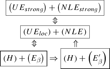
Theorem 4.6

(Grigor’yan and Hu) [GH00, Theorem 3.14]) Let $(M,d,\mu )$ be a metric measure space and let $\left( V_{\alpha }\right)$ hold. Let $(\mathcal {E},\mathcal {F})$ be a regular, strongly local Dirichlet form in $L^{2}(M,\mu )$. Then, the following equivalences are true:

$$\begin{aligned} \left( H\right) +\left( E_{\beta }^{\prime }\right)&\Leftrightarrow \left( G_{\beta }\right) \Leftrightarrow \left( H\right) +\left( R_{\beta }\right) \\&\Leftrightarrow \left( UE_{loc}\right) +(NLE) \\&\Leftrightarrow \left( UE_{strong}\right) +\left( NLE_{strong}\right) . \end{aligned}$$

We mention that condition $\left( V_{\alpha }\right)$ can be replaced by conditions $(\textit{VD})$ and $(\textit{RVD})$, the latter refers to the reverse doubling condition (cf. [GH00]).

Sketch of proof for Theorem 4.6 The proofs of Theorem 4.6 consists of two parts.

• Part One. Firstly, the following implications hold:

  

  In fact, by Theorem 4.3, we only need to show that

  $$\begin{aligned} \left( E_{\beta }\right)&\Rightarrow \left( E_{\beta }^{\prime }\right) ,\end{aligned}$$

  (4.11)
  $$\begin{aligned} \left( H\right) +\left( E_{\beta }^{\prime }\right)&\Longrightarrow \left( UE_{loc}\right) +(NLE). \end{aligned}$$

  (4.12)

  The implication (4.11) can be proved directly by using the probability argument, see [GH00, Theorem 3.14]. And the implication (4.12) can be done by showing the following

  $$\begin{aligned} \left( H\right) +\left( E_{\beta }^{\prime }\right)&\Rightarrow \left( \textit{FK}\right) \text { ([GT12, formula (3.17) and T.3.11])} \\ \left( E_{\beta }^{\prime }\right)&\Rightarrow \left( S_{\beta }\right) \text { (by [GHL00, formula (6.34)])} \\ \left( \textit{FK}\right) +\left( S_{\beta }\right)&\Rightarrow \left( UE_{loc}\right) \text { (by Theorem 3.8)} \\ \left( H\right) +\left( E_{\beta }^{\prime }\right)&\Rightarrow \left( NLE\right) \text { (by [GT12, Section 5.4]).} \end{aligned}$$

• Part Two. Secondly, we need to show that

  $$\begin{aligned} \left( H\right) +\left( E_{\beta }^{\prime }\right) \Leftrightarrow \left( G_{\beta }\right) \Leftrightarrow \left( H\right) +\left( R_{\beta }\right) . \end{aligned}$$

  This is the hard part. The cycle implications are obtained in [GH00, Section 8 ] as follows:

  $$\begin{aligned} \left( H\right) +\left( R_{\beta }\right) \Longrightarrow \left( G_{\beta }\right) \Longrightarrow \left( H\right) +\left( E_{\beta }^{\prime }\right) \Longrightarrow \left( H\right) +\left( R_{\beta }\right) . \end{aligned}$$

  One of the most challenging results (cf. [GH00, Lemma 5.7]) is to obtain an annulus Harnack inequality for the Green function, without assuming any specific properties of the metric $d$, unlike previously known similar results in [Bar05, GT02] where the geodesic property of the distance function was used. $\blacksquare$

4.2 Matching Upper and Lower Bounds

The purpose of this subsection is to improve both $\left( UE_{loc}\right)$ and $\left( NLE\right)$ in order to obtain matching upper and lower bounds for the heat kernel. The reason why $\left( UE_{loc}\right)$ and $\left( NLE\right)$ do not match, in particular, why $\left( NLE\right)$ contains no information about lower bound of $p_{t}\left( x,y\right)$ for distant $x,y$ is the lack of chaining properties of the distance function, that is an ability to connect any two points $x,y\in M$ by a chain of balls of controllable radii so that the number of balls in this chain is also under control.

For example, the chain condition considered above is one of such properties. If $\left( M,d\right)$ satisfies the chain condition, then as we have already mentioned, $\left( NLE\right)$ implies the full sun-Gaussian lower estimate by the chain argument and the semigroup property (see for example [GHL03, Corollary 3.5]).

Here we consider a setting with weaker chaining properties. For any $\varepsilon >0,$ we introduce a modified distance $d_{\varepsilon }\left( x,y\right)$ by

$$\begin{aligned} d_{\varepsilon }\left( x,y\right) =\inf _{\left\{ x_{i}\right\} \,\text {is } \varepsilon \text {-chain}}\sum _{i=1}^{N}d\left( x_{i},x_{i-1}\right) , \end{aligned}$$

(4.13)

where an $\varepsilon$ -chain is a sequence $\left\{ x_{i}\right\} _{i=0}^{N}$ of points in $M$ such that

$$\begin{aligned} x_{0}=x,\quad x_{N}=y,\quad {\text {and }}d(x_{i},x_{i-1})<\varepsilon \;\mathrm{{for\,\,all}}\;i=1,2,...,N. \end{aligned}$$

Clearly, $d_{\varepsilon }\left( x,y\right)$ is decreases as $\varepsilon$ increases and $d_{\varepsilon }\left( x,y\right) =d\left( x,y\right)$ if $\varepsilon >d\left( x,y\right)$. As $\varepsilon \downarrow$ $0$, $d_{\varepsilon }\left( x,y\right)$ increases and can go to $\infty$ or even become equal to $\infty$. It is easy to see that $d_{\varepsilon }\left( x,y\right)$ satisfies all properties of a distance function except for finiteness, so that it is a distance function with possible value $+\infty$.

It is easy to show that

$$\begin{aligned} d_{\varepsilon }\left( x,y\right) \asymp \varepsilon N_{\varepsilon }\left( x,y\right) , \end{aligned}$$

where $N_{\varepsilon }\left( x,y\right)$ is the smallest number of balls in a chain of balls of radius $\varepsilon$ connecting $x$ and $y$ (Fig. 7):

$N_{\varepsilon }$ can be regarded as the graph distance on a graph approximation of $M$ by an $\varepsilon$-net.

If $d$ is geodesic, then the points $\left\{ x_{i}\right\}$ of an $\varepsilon$-chain can be chosen on the shortest geodesic, whence $d_{\varepsilon }\left( x,y\right) =d\left( x,y\right)$ for any $\varepsilon >0$. If the distance function $d$ satisfies the chain condition, then one can choose in (4.13) an $\varepsilon$-chain so that $d\left( x_{i},x_{i+1}\right) \le C\frac{d\left( x,y\right) }{N}$, whence $d_{\varepsilon }\left( x,y\right) \le Cd\left( x,y\right)$. In general, $d_{\varepsilon }\left( x,y\right)$ may go to $\infty$ as $\varepsilon \rightarrow 0$, and the rate of growth of $d_{\varepsilon }\left( x,y\right)$ as $\varepsilon \rightarrow 0$ can be regarded as a quantitative description of the chaining properties of $d$.

Fig. 7

Chain of balls connecting $x$ and $y$

We need the following hypothesis

• $C_{\beta }$ (Chaining property) For all $x,y\in M$,

  $$\begin{aligned} \varepsilon ^{\beta -1}d_{\varepsilon }\left( x,y\right) \rightarrow 0\;\ \text {as }\varepsilon \rightarrow 0, \end{aligned}$$

  or equivalently,

  $$\begin{aligned} \varepsilon ^{\beta }N_{\varepsilon }\left( x,y\right) \rightarrow 0\;\text { as }\varepsilon \rightarrow 0. \end{aligned}$$

For $x\ne y$ we have $\varepsilon ^{\beta -1}d_{\varepsilon }\left( x,y\right) \rightarrow \infty$ as $\varepsilon \rightarrow \infty ,$ which implies under $\left( C_{\beta }\right)$ that for any $t>0,$ there is $\varepsilon =\varepsilon \left( t,x,y\right)$ satisfying the identity

$$\begin{aligned} \varepsilon ^{\beta -1}d_{\varepsilon }\left( x,y\right) =t \end{aligned}$$

(4.14)

(always take the maximal possible value of $\varepsilon$). If $x=y,$ then set $\varepsilon \left( t,x,x\right) =\infty .$

Theorem 4.7

(Grigor’yan, Telcs [GT12, Section 6]) Assume that all the hypothesis of Theorem 4.6 hold. If $\left( E_{\beta }\right) +\left( H\right)$ and $\left( C_{\beta }\right)$ are satisfied, then

$$\begin{aligned} p_{t}\left( x,y\right)&\asymp \frac{C}{t^{\alpha /\beta }}\exp \left( -c\left( \frac{d_{\varepsilon }^{\beta }(x,y)}{t}\right) ^{\frac{1}{\beta -1} }\right) \end{aligned}$$

(4.15)

$$\begin{aligned}&\asymp \frac{C}{t^{\alpha /\beta }}\exp \left( -cN_{\varepsilon }\left( x,y\right) \right) , \end{aligned}$$

(4.16)

where $\varepsilon =\varepsilon \left( t,x,y\right)$.

Since $d_{\varepsilon }\left( x,y\right) \ge d\left( x,y\right)$, the upper bound in (4.15) is an improvement of $\left( UE_{loc}\right)$; similarly the lower bound in (4.15) is an improvement of $\left( NLE\right)$. The proof of the upper bound in (4.15) follows the same line as the proof of $\left( UE_{loc}\right)$ with careful tracing all places where the distance $d\left( x,y\right)$ is used and making sure that it can be replaced by $d_{\varepsilon }\left( x,y\right)$. The proof of the lower bound in (4.16) uses $\left( NLE\right)$ and the semigroup identity along the chain with $N_{\varepsilon }$ balls connecting $x$ and $y$ . Finally, observe that (4.15) and (4.16) are equivalent, that is

$$\begin{aligned} N_{\varepsilon }\asymp \left( \frac{d_{\varepsilon }^{\beta }(x,y)}{t} \right) ^{\frac{1}{\beta -1}}, \end{aligned}$$

which follows by substituting here $N_{\varepsilon }\asymp d_{\varepsilon }/\varepsilon$ and $t=$ $\varepsilon ^{\beta -1}d_{\varepsilon }\left( x,y\right) .$

By Theorem 4.6, the same conclusion in Theorem 4.7 is true if $\left( E_{\beta }\right) +\left( H\right)$ is instead replaced by the one of conditions $\left( H\right) +\left( E_{\beta }^{\prime }\right) ,\left( G_{\beta }\right)$ and $\left( H\right) +\left( R_{\beta }\right)$.

Example 4.8

A good example to illustrate Theorem 4.7 is the class of post critically finite (p.c.f.) fractals. For connected p.c.f. fractals with regular harmonic structure, the heat kernel estimate (4.16) was proved by Hambly and Kumagai [HK99], see also [KS05, Theorem 5.2]. In this setting $d\left( x,y\right)$ is the resistance metric of the fractal $M$ and $\mu$ is the Hausdorff measure of $M$ of dimension $\alpha :=\dim _{H}M$. Hambly and Kumagai proved that $\left( V_{\alpha }\right)$ and $\left( E_{\beta }\right)$ are satisfied with $\beta =\alpha +1$. The condition $\left( C_{\beta }\right)$ follows from their estimate

$$\begin{aligned} N_{\varepsilon }\left( x,y\right) \le C\left( \frac{d\left( x,y\right) }{ \varepsilon }\right) ^{\beta /2}, \end{aligned}$$

because

$$\begin{aligned} \varepsilon ^{\beta }N_{\varepsilon }\left( x,y\right) \le Cd\left( x,y\right) ^{\beta /2}\varepsilon ^{\beta /2}\rightarrow 0\;\text {as } \varepsilon \rightarrow 0. \end{aligned}$$

The Harnack inequality $\left( H\right)$ on p.c.f. fractals was proved by Kigami [Kig01, Proposition 3.2.7, p.78]. Hence, Theorem 4.7 applies and gives the estimates (4.15) and (4.16).

The estimate (4.16) means that the diffusion process goes from $x$ to $y$ in time $t$ in the following way. The process firstly “computes” the value $\varepsilon \left( t,x,y\right)$, secondly “detects” a shortest chain of $\varepsilon$-balls connecting $x$ and $y$, and then goes along that chain (Fig. 8).

Fig. 8

Two shortest chains of $\varepsilon$-ball for two distinct values of $\varepsilon$ provide different routes for the diffusion from $x$ to $y$ for two distinct values of $t$

This phenomenon was first observed by Hambly and Kumagai on p.c.f. fractals, but it seems to be generic. Hence, to obtain matching upper and lower bounds, one needs in addition to the usual hypotheses also the following information, encoded in the function $N_{\varepsilon }\left( x,y\right)$: the graph distance between $x$ and $y$ on any $\varepsilon$-net approximation of $M$.

Example 4.9

(Computation of $\varepsilon$) Assume that the following bound is known for all $x,y\in M$ and $\varepsilon >0$

$$\begin{aligned} N_{\varepsilon }\left( x,y\right) \le C\left( \frac{d\left( x,y\right) }{ \varepsilon }\right) ^{\gamma }, \end{aligned}$$

where $0<\gamma <\beta$, so that $\left( C_{\beta }\right)$ is satisfied (since $N_{\varepsilon }\ge d\left( x,y\right) /\varepsilon$, one must have $\gamma \ge 1$). Since by (4.14) we have $\varepsilon ^{\beta }N_{\varepsilon }\asymp t$, it follows that

$$\begin{aligned} \varepsilon ^{\beta }\left( \frac{d\left( x,y\right) }{\varepsilon }\right) ^{\gamma }\ge ct, \end{aligned}$$

whence

$$\begin{aligned} \varepsilon \ge c\left( \frac{t}{d\left( x,y\right) ^{\gamma }}\right) ^{ \frac{1}{\beta -\gamma }}. \end{aligned}$$

Consequently, we obtain

$$\begin{aligned} N_{\varepsilon }\left( x,y\right) \le Cd\left( x,y\right) ^{\gamma }\varepsilon ^{-\gamma }\le Cd\left( x,y\right) ^{\gamma }\left( \frac{ d\left( x,y\right) ^{\gamma }}{t}\right) ^{\frac{\gamma }{\beta -\gamma } }=C\left( \frac{d\left( x,y\right) ^{\beta }}{t}\right) ^{\frac{\gamma }{ \beta -\gamma }}, \end{aligned}$$

and so

$$\begin{aligned} p_{t}\left( x,y\right) \ge \frac{c}{t^{\alpha /\beta }}\exp \left( -\left( \frac{d\left( x,y\right) ^{\beta }}{ct}\right) ^{\frac{\gamma }{\beta -\gamma }}\right) . \end{aligned}$$

Similarly, the lower estimate of $N_{\varepsilon }$

$$\begin{aligned} N_{\varepsilon }\left( x,y\right) \ge c\left( \frac{d\left( x,y\right) }{ \varepsilon }\right) ^{\gamma } \end{aligned}$$

implies an upper bound for the heat kernel

$$\begin{aligned} p_{t}\left( x,y\right) \le \frac{C}{t^{\alpha /\beta }}\exp \left( -\left( \frac{d\left( x,y\right) ^{\beta }}{Ct}\right) ^{\frac{\gamma }{\beta -\gamma }}\right) . \end{aligned}$$

Remark 4.10

Assume that $\left( V_{\alpha }\right)$ holds and all balls in $M$ of radius $\ge r_{0}$ are connected, for some $r_{0}>0$. We claim that $\left( C_{\beta }\right)$ holds with any $\beta >\alpha$. The $\alpha$-regularity of measure $\mu$ implies, by the classical ball covering argument, that any ball $B_{r}$ of radius $r$ can be covered by at most $C\left( \frac{r}{\varepsilon }\right) ^{\alpha }$ balls of radii $\varepsilon \in \left( 0,r\right)$. Consequently, if $B_{r}$ is connected then any two points $x,y\in B_{r}$ can be connected by a chain of $\varepsilon$-balls containing at most $C\left( \frac{r}{\varepsilon } \right) ^{\alpha }$ balls, so that

$$\begin{aligned} N_{\varepsilon }\left( x,y\right) \le C\left( \frac{r}{\varepsilon }\right) ^{\alpha }. \end{aligned}$$

Since any two points $x,y\in M$ are contained in a connected ball $B_{r}$ (say, with $r=r_{0}+d\left( x,y\right)$), we obtain

$$\begin{aligned} \varepsilon ^{\beta }N_{\varepsilon }\left( x,y\right) \le C\varepsilon ^{\beta -\alpha }r^{\alpha }\rightarrow 0 \end{aligned}$$

as $\varepsilon \rightarrow 0$, which was claimed.

4.3 Further Results

We discuss here some consequences and extensions of the above results. For this, we introduce two-sided estimates of the heat kernel.

• $(ULE_{loc})$ (Upper and lower estimates) The heat kernel $p_{t}\left( x,y\right)$ exists and satisfies

  $$\begin{aligned} p_{t}\left( x,y\right) \asymp \frac{C}{t^{\alpha /\beta }}\exp \left( -c\left( \frac{d^{\beta }(x,y)}{t}\right) ^{\frac{1}{\beta -1}}\right) . \end{aligned}$$

  (4.17)

Theorem 4.11

Let $(M,d,\mu )$ be a metric measure space, and let $(\mathcal { E},\mathcal {F})$ be a regular, conservative Dirichlet form in $L^{2}(M,\mu )$ . If $\left( M,d\right)$ satisfies the chain condition, then the following equivalences take place:

$$\begin{aligned} \left( V_{\alpha }\right) +\left\{ \begin{array}{l} \left( E_{\beta }\right) +\left( H\right) \\ \left( E_{\beta }^{\prime }\right) +\left( H\right) \\ \left( R_{\beta }\right) +\left( H\right) \\ \left( G_{\beta }\right) \end{array} \right. +(\text {locality})\Longleftrightarrow (ULE_{loc}), \end{aligned}$$

where condition $($locality$)$ means that $(\mathcal {E},\mathcal {F})$ is local.

Remark 4.12

Observe that if $(\mathcal {E},\mathcal {F})$ is regular, conservative and local, then $(\mathcal {E},\mathcal {F})$ is strongly local; this is easily seen by using the Beuling-Deny decomposition [FOT11, Theorem 3.2.1, p. 120] and by noting that both killing and jump measures disappear.

Remark 4.13

Observe also that $\left( V_{\alpha }\right) +(NLE)+$ $\left( \text {chain condition}\right)$ implies that the off-diagonal lower estimate

$$\begin{aligned} p_{t}\left( x,y\right) \ge \frac{C^{\prime }}{t^{\alpha /\beta }}\exp \left( -c^{\prime }\left( \frac{d^{\beta }(x,y)}{t}\right) ^{\frac{1}{\beta -1}}\right) \end{aligned}$$

(4.18)

for $\mu$-almost all $x,y\in M$ and all $t>0$, see for example [GHL08, Proposition 3.1] or [Bar98], [GHL03, Corollary 3.5].

Sketch of proof for Theorem 4.11 (1) “$\Rightarrow$”.

Let us show the implication

$$\begin{aligned} \left( V_{\alpha }\right) +\left( E_{\beta }\right) +\left( H\right) +(\text { locality})\Rightarrow (ULE_{loc}). \end{aligned}$$

(4.19)

Indeed, by Remark 4.12, we have that $(\mathcal {E},\mathcal {F})$ is strongly local. Now, using Theorem 4.3, we obtain $\left( UE_{loc}\right) +(NLE).$ Using Remark 4.13, we see that (4.18) holds, showing that $(ULE_{loc})$ is true.

Similarly, using Theorem 4.6, we obtain the other three implications “$\Rightarrow$”.

(2) “$\Leftarrow$”.

Let us show the opposite implication

$$\begin{aligned} (ULE_{loc})\Rightarrow \left( V_{\alpha }\right) +\left( E_{\beta }\right) +\left( H\right) +(\text {locality}). \end{aligned}$$

(4.20)

Indeed, note that

$$\begin{aligned} (ULE_{loc})&\Rightarrow \left( V_{\alpha }\right) \text { (by Theorem 2.2)} \\ \left( UE_{loc}\right)&\Rightarrow (\text {locality})\text { (by Theorem 2.14)} \\ \left( UE_{loc}\right) +\left( NLE\right)&\Rightarrow \left( E_{\beta }\right) +\left( H\right) \text { (by Theorem 4.3)} \end{aligned}$$

showing that the implication (4.20) holds.

Similarly, all the other three implications “$\Longleftarrow$” also hold. $\blacksquare$

Remark 4.14

The implication (4.19) can also be proved by using Theorem 4.7 and the fact that $d_{\varepsilon }\asymp d$.

Conjecture 4.15

The condition $\left( E_{\beta }\right)$ above may be replaced by

In fact, $\left( E_{\beta }\right)$ in all statements can be replaced by the resistance condition:

where $B_{r}=B\left( x,r\right)$. In the strongly recurrent case $\alpha <\beta ,$ it alone implies the elliptic Harnack inequality $\left( H\right)$ so that two sided heat kernel estimates are equivalent to $\left( V_{\alpha }\right) +\left( R_{\beta }\right)$ as was proved by Barlow, Coulhon, Kumagai [BCK05] (in a setting of graphs) and was discussed in M. Barlow’s lectures.

An interesting (and obviously hard) question is the characterization of the elliptic Harnack inequality $(H)$ in more geometric terms—so far nothing is known, not even a conjecture.

One can consider also a parabolic Harnack inequality $(\textit{PHI})$, which uses caloric functions instead of harmonic functions. Then in a general setting and assuming the volume doubling condition $(\textit{VD})$ (instead of $\left( V_{\alpha }\right)$), the following holds (cf. [BGK12]):

$$\begin{aligned} (\textit{PHI}) \Leftrightarrow \left( UE_{loc}\right) +\left( NLE\right) . \end{aligned}$$

On the other hand, $(\textit{PHI})$ is equivalent to

$$\begin{aligned} \text {Poincar}\acute{\mathrm{e}} \,\text {inequality} + \text {cutoff Sobolev inequality,} \end{aligned}$$

see [BBK06].

Conjecture 4.16

The cutoff Sobolev inequality here can be replaced by $\left( \lambda _{\beta }\right)$ and/or $\left( R_{\beta }\right) .$

5 Upper Bounds for Jump Processes

We have investigated above the heat kernel for the local Dirichlet form. In this section we shall study the non-local Dirichlet form and present the equivalence conditions for upper bounds of the associated heat kernel. As an interesting example, we discuss the heat kernel estimates for effective metric spaces.

A non-local Dirichlet form will give arise to a jump process, that is, the trajectories of this process are discontinuous, as we have already seen for a symmetric stable process of index $\beta$ (Lévy process). And the heat kernel decays at a polynomial rate (cf. 1.2), instead of an exponential rate as for a local Dirichlet form.

Jump process have found various applications in science. For instance, a Lévy flight is a jump process and can be used to describe animal foraging patterns, the distribution of human travel and some aspects of earthquake behavior (cf. [BBW08]).

5.1 Upper Bounds for Non-local Dirichlet Forms

The techniques for obtaining heat kernel bounds for non-local Dirichlet forms has been developed by a number of authors, see for example [BBCK09, BGK09, BL02, CK03, CK08] and the references therein. The basic approach to obtaining heat kernel upper estimates used in these papers consists of the two steps. The first step is to obtain the heat kernel upper bounds for a truncated Dirichlet form, that is, in the case when the jump density $J\left( x,y\right)$ has a bounded range. In this case one uses the Davies method as it was presented in the seminal work [CKS87] and where the cut-off functions of form $\left( \lambda -d(x_{0},x)\right) _{+}$ were used (where $\lambda$ is a positive constant). This method can be used as long as the cut-off functions belong to the domain of the Dirichlet form, which is the case only when $\beta <2$ (hence, if $\beta \ge 2$ then this method does not work).

The second step is to obtain heat kernel estimates for the original Dirichlet form by comparing the heat semigroup of the truncated Dirichlet form with the original heat semigroup. We remark that while the first step was done by purely analytic means, the second step in the above-mentioned papers used a probabilistic argument.

Here we describe an alternative new approach of [GHL00] for obtaining upper bounds.

Recall that by a theorem of Beurling and Deny, any regular conservative Dirichlet form admits a decomposition

$$\begin{aligned} \mathcal {E}(u,v)=\mathcal {E}^{(L)}(u,v)+\mathcal {E}^{(J)}(u,v), \end{aligned}$$

(5.1)

where $\mathcal {E}^{(L)}$ is a local part and

$$\begin{aligned} \mathcal {E}^{\left( J\right) }\left( u,v\right) =\mathop {\displaystyle \int \int }\limits _{M\times M\setminus \mathop {{\mathrm{diag}}}\nolimits }\left( u(x)-u(y)\right) \left( v(x)-v(y)\right) dj(x,y) \end{aligned}$$

(5.2)

is a jump part with a jump measure $j$ defined on $M\times M\setminus \mathop {{\mathrm{diag}}}\nolimits$. In our setting the jump measure $j$ will have a density with respect to $\mu \times \mu$, which will be denoted by $J\left( x,y\right) ,$ and so the jump part $\mathcal {E}^{\left( J\right) }$ becomes

$$\begin{aligned} \mathcal {E}^{\left( J\right) }\left( u,v\right) =\mathop {\mathop {\displaystyle \int \int }}\limits _{M\times M}\left( u(x)-u(y)\right) \left( v(x)-v(y)\right) J(x,y)d\mu (y)d\mu (x). \end{aligned}$$

(5.3)

We introduce the following hypothesis.

• $\left( \mathbf {V}_{\mathbf {\le }}\right)$ (Upper $\alpha$- regularity) For all $x\in M$ and all $r>0$,

  $$\begin{aligned} V(x,r)\le Cr^{\alpha }. \end{aligned}$$

• $\mathbf {(UE)}$ (Upper estimate of non-local type) The heat kernel $p_{t}$ exists and satisfies the off-diagonal upper estimate

  $$\begin{aligned} p_{t}(x,y)\le \frac{C}{t^{\alpha /\beta }}\left( 1+\frac{d(x,y)}{t^{1/\beta }}\right) ^{-\left( \alpha +\beta \right) } \end{aligned}$$

  for all $t>0$ and $\mu$-almost all $x,y\in M.$

• $\mathbf {(J}_{\mathbf {\le }}\mathbf {)}$ (Upper bound of jump density) The jump density exists and admits the estimate

  $$\begin{aligned} J(x,y)\le Cd(x,y)^{-(\alpha +\beta )}, \end{aligned}$$

  for $\mu$-almost all $x,y\in M$.

• $\mathbf {(T}_{strong}\mathbf {)}$ (Strong tail estimate) There exist constants $c>0$ and $\beta >0$ such that, for all balls $B=B(x_{0},r)$ and for all $t>0$,

  $$\begin{aligned} P_{t}\mathbf {1}_{B^{c}}(x)\le \frac{ct}{r^{\beta }}\;\text {for }\mu \text { -almost all }x\in \frac{1}{4}B. \end{aligned}$$

  Clearly, we have that $\left( T_{\exp }\right) \Rightarrow \left( T_{strong}\right) \Rightarrow \left( T_{\beta }\right) .$

We now state the main technical result of [GHL00].

Theorem 5.1

(Grigor’yan et al. [GHL00]) Let $(M,d,\mu )$ be a metric measure space with precompact balls, and let $(\mathcal {E},\mathcal {F})$ be a regular conservative Dirichlet form in $L^{2}\left( M,\mu \right)$ with jump density $J$. Then the following implication holds:

$$\begin{aligned} \left( V_{\le }\right) +\left( \textit{DUE}\right) +(J_{\le })+\left( S_{\beta }\right) \Rightarrow \left( UE\right) . \end{aligned}$$

(5.4)

We remark that by [GHL03, Theorem 3.2], if $(\mathcal {E},\mathcal {F})$ is conservative then

$$\begin{aligned} \left( V_{\le }\right) +(UE)\Rightarrow \left( V_{\alpha }\right) . \end{aligned}$$

Hence, the hypotheses of Theorem 5.1 imply that $\mu$ is $\alpha$-regular.

Sketch of proof for Theorem 5.1 We sketch the ideas of the proof.

• Step $1$ . We decompose $\mathcal {E}(u)$ into two parts:

  $$\begin{aligned} \mathcal {E}(u)=\mathcal {E}^{(\rho )}(u)+\int \limits _{M}\int \limits _{M\setminus B(x,\rho )}\left( u(x)-u(y)\right) ^{2}J(x,y)d\mu (y)d\mu (x), \end{aligned}$$

  where $\rho \in \left( 0,\infty \right)$ is any fixed number. Then the form $\left( \mathcal {E}^{\left( \rho \right) },\mathcal {F}\right)$ can be extended to a regular Dirichlet form $\left( \mathcal {E}^{\left( \rho \right) },\mathcal {F}^{\left( \rho \right) }\right) .$ Indeed, since using condition $(J_{\le }),$

  $$\begin{aligned} \mathop {{\mathrm{esup}}}_{x\in M}\int \limits _{B(x,\rho )^{c}}J(x,y)d\mu (y)<\infty , \end{aligned}$$

  the form $\left( \mathcal {E}^{(\rho )},\mathcal {F}\right)$ is closable, and its closure $\left( \mathcal {E}^{\left( \rho \right) },\mathcal {F}^{\left( \rho \right) }\right)$ in $L^{2}$ is a regular Dirichlet form in $L^{2}.$ Note that $\left( \mathcal {E}^{\left( \rho \right) },\mathcal {F}^{\left( \rho \right) }\right)$ is $\rho$ -local (non-local): $\mathcal {E} ^{\left( \rho \right) }(f,g)=0$ for any two functions $f,g\in \mathcal {F} ^{\left( \rho \right) }$ with compact supports such that

  $$\begin{aligned} \mathop {{\mathrm{dist}}} \left( \mathop {{\mathrm{supp}}} f, \mathop {{\mathrm{supp}}} g\right) >\rho . \end{aligned}$$

• Step $2$. We need to obtain upper estimates of the heat kernel $q_{t}(x,y)$ of the truncated Dirichlet form $\left( \mathcal {E}^{(\rho )},\mathcal {F}^{(\rho )}\right)$. Indeed, conditions $(\textit{DUE}),\left( J_{\le }\right) ,(S_{\beta })$ and $\left( V_{\le }\right)$ imply the following estimate of $q_{t}(x,y):$

  $$\begin{aligned} q_{t}(x,y)\le \frac{C}{t^{\alpha /\beta }}\exp \left( 4\rho ^{-\beta }t\right) \exp \left( -c\left( \frac{d(x,y)}{\rho }\wedge \frac{\rho }{ t^{1/\beta }}\right) \right) \end{aligned}$$

  (5.5)

  for all $t>0$ and $\mu$-almost all $x,y\in M$, where constants $C,c>0$ depend on the constants in the hypotheses but are independent of $\rho .$ This can be done with a certain amount of effort, by using the bootstrapping technique where the comparison inequality [GHL10, Corollary 4.8, Remark 4.10] for heat semigroups play an important rôle.

• Step $3$ . Next we apply the following useful inequality between two heat kernels:

  $$\begin{aligned} p_{t}(x,y)\le q_{t}(x,y)+2t\mathop {{\mathrm{esup}}}_{x\in M,y\in B(x,\rho )^{c}}J(x,y) \end{aligned}$$

  (5.6)

  for all $t>0$ and almost all $x,y\in M;$ this inequality follows from the parabolic maximum principle alone. Therefore, by choosing an appropriate $\rho$, it follows from (5.5), (5.6) that, for any real $n\ge 0,$

  $$\begin{aligned} p_{t}(x,y)\le \frac{c(n)}{t^{\alpha /\beta }}\left( 1+\frac{d(x,y)}{ t^{1/\beta }}\right) ^{-\frac{\left( \alpha +\beta \right) n}{n+\alpha +\beta }} \end{aligned}$$

  (5.7)

  for almost all $x,y\in M$ and all $t>0$.

  Note that (5.7) is nearly close to our desired estimate $\left( UE\right) .$ However, one can not just obtain $\left( UE\right)$ by directly taking the limit as $n\rightarrow \infty$, since we do not know whether the coefficient $c(n)$ is bounded uniformly in $n$. We need the second iteration.

• Step $4$ . Finally, we will obtain $(UE)$ by a self-improvement of (5.7). Indeed, one can use (5.7) to obtain

  $$\begin{aligned} \int \limits _{B(x,r)^{c}}p_{t}(x,y)d\mu (y)\le C(n)\left( rt^{-1/\beta }\right) ^{-\theta }, \end{aligned}$$

  where $\theta =\frac{n\beta -\alpha \left( \alpha +\beta \right) }{n+\alpha +\beta }\in (0,\beta )$ (note that this estimate is sharper than condition $\left( S_{\beta }\right)$), and then repeating the above procedure, we arrive at $\left( UE\right)$. $\blacksquare$

Now we can state some equivalences for $\left( UE\right)$.

Theorem 5.2

(Grigor’yan et al. [GHL00]) Let $(M,d,\mu )$ be a metric measure space with precompact balls, and let $(\mathcal {E},\mathcal {F})$ be a regular conservative Dirichlet form in $L^{2}\left( M,\mu \right)$ with jump density $J$. If $\left( V_{\le }\right)$ holds, then the following equivalences are true:

$$\begin{aligned} \left( UE\right)&\Leftrightarrow \left( UE\Phi \right) +(J_{\le }) \nonumber \\&\Leftrightarrow \left( \textit{DUE}\right) +(J_{\le })+\left( T_{\beta }\right) \nonumber \\&\Leftrightarrow \left( \textit{DUE}\right) +(J_{\le })+\left( S_{\beta }\right) \nonumber \\&\Leftrightarrow \left( \textit{DUE}\right) +(J_{\le })+\left( T_{strong}\right) . \end{aligned}$$

(5.8)

Proof

Observe that the implication $\left( UE\right) \Rightarrow (J_{\le })$ holds by [BGK09, p. 150], and $\left( UE\right) \Rightarrow \left( UE\Phi \right)$ is trivial by taking $\Phi (s)=\left( 1+s\right) ^{-\left( \alpha +\beta \right) }$. The implication $\left( UE\Phi \right) \Rightarrow \left( \textit{DUE}\right)$ is obvious. The implication $\left( UE\Phi \right) \Rightarrow \left( T_{\beta }\right)$ was proved in (3.10) (see also [GHL03, formula (3.6), p. 2072]). Since $(\mathcal {E},\mathcal {F})$ is conservative, the equivalence $\left( T_{\beta }\right) \Leftrightarrow \left( S_{\beta }\right)$ holds by [GH08, Theorem 3.1, p. 96]. By Theorem 5.1 we have

$$\begin{aligned} \left( \textit{DUE}\right) +(J_{\le })+\left( S_{\beta }\right) \Rightarrow \left( UE\right) , \end{aligned}$$

which closes the cycle of implications, thus proving the first three equivalences.

Finally, the implication $\left( UE\right) \Rightarrow \left( T_{strong}\right)$ is true by using (3.10), and hence

$$\begin{aligned} \left( UE\right)&\Rightarrow \left( \textit{DUE}\right) +(J_{\le })+\left( T_{strong}\right) \\&\Rightarrow \left( \textit{DUE}\right) +(J_{\le })+\left( T_{\beta }\right) \Rightarrow \left( UE\right) , \end{aligned}$$

which finishes the proof. $\blacksquare$

Remark 5.3

The upper estimate $\left( UE\right)$ is best possible for non-local forms in the following sense: if the heat kernel $p_{t}$ satisfies the estimate

$$\begin{aligned} p_{t}(x,y)\le \frac{1}{t^{\alpha /\beta }}\Phi \left( \frac{d(x,y)}{ t^{1/\beta }}\right) \end{aligned}$$

for all $t>0$ and $\mu$-almost all $x,y\in M$, where $\Phi$ is a continuous decreasing function on $[0,+\infty ),$ then necessarily

$$\begin{aligned} \Phi \left( s\right) \ge c\left( 1+s\right) ^{-\left( \alpha +\beta \right) } \end{aligned}$$

for some $c>0$ (see Theorem 2.14).

Remark 5.4

Under the standing assumptions of Theorem 5.2, the following equivalence is true

$$\begin{aligned} \left( UE_{loc}\right) \Leftrightarrow \left( \textit{DUE}\right) + (\text {``locality''})+\left( S_{\beta }\right) . \end{aligned}$$

Indeed, since $\left( UE_{loc}\right)$ is stronger than $\left( UE\right)$ , it implies $\left( \textit{DUE}\right)$ and $\left( S_{\beta }\right)$ by Theorem 5.2. Next, $\left( UE_{loc}\right) \Rightarrow$(“locality”) by Theorem 2.14 above. The opposite implication

$$\begin{aligned} \left( \textit{DUE}\right) +\text {(``locality'')}+\left( S_{\beta }\right) \Rightarrow \left( UE_{loc}\right) \end{aligned}$$

was stated in Theorem 3.8.

In order to state some consequence of Theorem 5.2, we need the following Proposition.

Define first the following condition:

• $\mathbf {(J}_{\mathbf {\ge }}\mathbf {)}$ (Lower bound of jump density) There exist constants $C,\alpha ,\beta >0$ such that, for $\mu$ -almost all $x\ne y,$

  $$\begin{aligned} J(x,y)\ge C^{-1}d(x,y)^{-(\alpha +\beta )}. \end{aligned}$$

Proposition 5.5

Let $(M,d,\mu )$ be a metric measure space, and let $(\mathcal {E}, \mathcal {F})$ be a regular Dirichlet form in $L^{2}\left( M,\mu \right)$ with jump density $J$. Then

$$\begin{aligned} (V_{\alpha })+(J_{\ge })\Rightarrow \left( \textit{DUE}\right) . \end{aligned}$$

(5.9)

Proof

As was proved in [HuK06, Theorem 3.1], under $\left( V_{\alpha }\right)$ the following inequality holds for all non-zero functions $u\in L^{1}\cap L^{2}$:

$$\begin{aligned} \int \limits _{M}\int \limits _{M}\frac{\left( u\left( x\right) -u\left( y\right) \right) ^{2} }{d\left( x,y\right) ^{\alpha +\beta }}d\mu \left( x\right) d\mu \left( y\right) \ge c||u||_{2}^{2(1+\beta /\alpha )}\left\| u\right\| _{1}^{-2\beta /\alpha }, \end{aligned}$$

where $c$ is a positive constant. Using (5.1), (5.3) and $\left( J_{\ge }\right)$ we obtain

$$\begin{aligned} \mathcal {E}\left( u\right)&= \mathcal {E}^{(L)}\left( u\right) +\mathcal {E} ^{(J)}\left( u\right) \\&\ge C\int \limits _{M}\int \limits _{M}\frac{\left( u\left( x\right) -u\left( y\right) \right) ^{2}}{d\left( x,y\right) ^{\alpha +\beta }}d\mu \left( x\right) d\mu \left( y\right) \\&\ge c||u||_{2}^{2(1+\beta /\alpha )}\left\| u\right\| _{1}^{-2\beta /\alpha } \end{aligned}$$

for all $u\in \mathcal {F}\cap L^{1}$. Hence, $\left( \textit{DUE}\right)$ follows by Theorem 3.6. $\blacksquare$

We obtain the following consequence of Theorem 5.2.

Theorem 5.6

(Grigor’yan et al. [GHL00]) Let $(M,d,\mu )$ be a metric measure space with precompact balls, and let $(\mathcal {E},\mathcal {F})$ be a regular conservative Dirichlet form in $L^{2}\left( M,\mu \right)$ with jump density $J$. If $\left( V_{\alpha }\right)$ holds and $J(x,y)\asymp d(x,y)^{-(\alpha +\beta )}$, then

$$\begin{aligned} \left( UE\right) \Leftrightarrow \left( S_{\beta }\right) . \end{aligned}$$

(5.10)

Proof

Let us show that $\left( S_{\beta }\right) \Rightarrow \left( UE\right) .$ Indeed, $\left( \textit{DUE}\right)$ holds by Proposition 5.5. Hence, $\left( UE\right)$ is satisfied by Theorem 5.2. The opposite implication $\left( UE\right) \Rightarrow \left( S_{\beta }\right)$ holds also by Theorem 5.2. $\blacksquare$

Therefore, if $\left( V_{\alpha }\right)$ holds and $J(x,y)\asymp d(x,y)^{-(\alpha +\beta )},$ then in order to obtain off-diagonal upper bounds of heat kernels, one needs only to verify the survival condition $\left( S_{\beta }\right) .$ In the sequel, we will show that the survival condition $\left( S_{\beta }\right)$ holds for a class of measure spaces with effective resistance metrics.

5.2 Upper Bounds Using Effective Resistance

We will show how Theorem 5.2 can be applied for a certain class of metric measure spaces with effective resistance.

Let $\left( \mathcal {E},\mathcal {F}\right)$ be a regular Dirichlet form in $L^{2}\left( M,\mu \right)$ as before. Recall that the effective resistance $R(A,B)$ between two disjoint non-empty closed subsets $A$ and $B$ of $M$ is defined by

$$\begin{aligned} R(A,B)^{-1}=\inf \left\{ \mathcal {E}\left( u\right) :\text { }u\in \mathcal {F} \cap C_{0},\text { }u|_{A}=1\text { and }u|_{B}=0\right\} . \end{aligned}$$

(5.1)

It follows from (5.1) that, for any fixed $A$, $R(A,B)$ is a non-increasing function of $B$. Denote by

$$\begin{aligned} R(x,B):=R(\{x\},B)\text { and }R(x,y):=R(\{x\},\{y\}). \end{aligned}$$

In general, it may happen that $R(x,y)=\infty$ for some points $x,y\in M$. Below we will exclude this case.

Fix a parameter $\gamma >0,$ and introduce conditions $\left( R_{1}\right)$ and $\left( R_{2}\right)$.

• $\mathbf {(R}_{1}\mathbf {):}$ For all $u\in \mathcal {F}\cap C_{0}(M)$ and all $x,y\in M$, the following inequality holds:

  $$\begin{aligned} \left| u(x)-u(y)\right| ^{2}\le Cd(x,y)^{\gamma }\mathcal {E}\left( u\right) . \end{aligned}$$

• $\mathbf {(R}_{2}\mathbf {):}$ For all $x\in M$ and $r>0$,

  $$\begin{aligned} R(x,B(x,r)^{c})\ge C^{-1}r^{\gamma }. \end{aligned}$$

Theorem 5.7

(Grigor’yan et al. [GHL00]) Let $\left( \mathcal {E},\mathcal {F}\right)$ be a regular Dirichlet form in $L^{2}\left( M,\mu \right)$. Then

$$\begin{aligned} \left( V_{\alpha }\right) +\left( R_{1}\right) +\left( R_{2}\right) \Rightarrow \left( S_{\beta }\right) +(\textit{DUE}), \end{aligned}$$

where $\beta =\alpha +\gamma$. Consequently, under the standing conditions $\left( V_{\alpha }\right) +\left( R_{1}\right) +\left( R_{2}\right)$, we have that

$$\begin{aligned} (UE)\Leftrightarrow (J_{\le }). \end{aligned}$$

(5.2)

Sketch of proof for Theorem 5.7 The proof consists of the following five steps.

• Step $1$. For any ball $B:=B(x_{0},r)$, using conditions $\left( R_{1}\right)$ and $\left( R_{2}\right) ,$ we can obtain the two-sided estimate of the Green functions $g_{B}(x,y):$

  $$\begin{aligned} \sup _{x,y\in B}g_{B}(x,y)&\le Cr^{\gamma }, \end{aligned}$$

  (5.3)
  $$\begin{aligned} \inf _{y\in B(x_{0},\eta r)}g_{B}(x_{0},y)&\ge C^{-1}r^{\gamma }, \end{aligned}$$

  (5.4)

  where $C>0$ and $\eta \in (0,1).$

• Step $2$. Therefore, under condition $\left( V_{\alpha }\right)$, it follows from (5.3), (5.4) that condition $\left( E_{\beta }^{\prime }\right)$ holds:

  $$\begin{aligned} \mathop {{\mathrm{esup}}}_{B}E^{B}&\le Cr^{\alpha +\gamma }, \end{aligned}$$

  (5.5)
  $$\begin{aligned} \underset{\delta _{1}B}{\mathop {{\mathrm{einf}}}}E^{B}&\ge C^{-1}r^{\alpha +\gamma }, \end{aligned}$$

  (5.6)

  where $E^{B}$ is the weak solution of the Poisson-type equation (4.7) as before, and $C>0$ and $\delta _{1}\in (0,1/2)$.

• Step $3$. To show condition $\left( S_{\beta }\right)$, observe that, for all $t>0$ and $\mu$-almost all $x\in B,$

  $$\begin{aligned} P_{t}^{B}1_{B}(x)\ge \frac{E^{B}(x)-t}{\left\| E^{B}\right\| _{\infty }}, \end{aligned}$$

  (5.7)

  which follows by using the parabolic maximum principle, nothing else. Hence, using (5.5), (5.6),

  $$\begin{aligned} P_{t}^{B}1_{B}(x)&\ge \frac{E^{B}(x)-t}{\left\| E^{B}\right\| _{\infty }} \\&\ge c-c_{1}tr^{-\beta } \\&\ge \frac{c}{2}, \end{aligned}$$

  for all $t>0$ and $\mu$-almost all $x\in$ $B(x_{0},\delta _{1}r)$, provided that $tr^{-\beta }$ is small enough, thus proving $\left( S_{\beta }\right)$.

• Step $4$. We show that $\left( R_{1}\right) \Rightarrow (\textit{DUE})$. Consider a function $f\in \mathcal {F}\cap C_{0}(\Omega )$ normalized so that $\sup |f|=1,$ and let $x\in \Omega$ be a point such that $|f(x)|=1$. Let $r$ be the largest radius such that $B(x,r)\subset \Omega$. Then the ball $B\left( x,2r\right)$ is not covered by $\Omega$ so that there exists a point $y\in B\left( x,2r\right) \setminus \Omega$ (note that $M$ is unbounded by condition $\left( V_{\alpha }\right)$). In particular, $y\notin \mathop {{\mathrm{supp}}}f$ (see Fig. 9). Noting that $\mathcal {E}^{(J)}\left( f\right) \le \mathcal {E}\left( f\right)$ and by the $\alpha$-regularity of $\mu$

  $$\begin{aligned} r\le C\left[ \mu \left( B(x,r)\right) \right] ^{1/\alpha }\le C\left[ \mu \left( \Omega \right) \right] ^{1/\alpha }, \end{aligned}$$

  we obtain from $\left( R_{1}\right)$ that

  $$\begin{aligned} 1&= |f(y)-f(x)|^{2} \\&\le Cd(y,x)^{\beta -\alpha }\mathcal {E}^{(J)}\left( f\right) \\&\le C\left( 2r\right) ^{\beta -\alpha }\mathcal {E}\left( f\right) \le C2^{\beta -\alpha }\left[ \mu \left( \Omega \right) \right] ^{\beta /\alpha -1}\mathcal {E}\left( f\right) . \end{aligned}$$

  Since $\left\| f\right\| _{2}^{2}\le \mu \left( \Omega \right)$, it follows that

  $$\begin{aligned} \frac{\mathcal {E}\left( f\right) }{\left\| f\right\| _{2}^{2}}\ge c \left[ \mu \left( \Omega \right) \right] ^{-\beta /\alpha }, \end{aligned}$$

  for some $c>0$, thus proving the Faber-Krahn inequality. Hence, condition $(\textit{DUE})$ follows by using Theorem 3.6.

• Step $5$. Finally, with a certain amount of effort [GHL00, Proposition 6.5, Lemma 6.4], one can show that

  $$\begin{aligned} \left( R_{1}\right) +\left( R_{2}\right) \Rightarrow \text {conservativeness of }\left( \mathcal {E},\mathcal {F}\right) . \end{aligned}$$

  Therefore, the equivalence (5.2) follows directly by using Theorem 5.2.

Fig. 9

Points x, y

References

Andres, S., Barlow, M.: Energy inequalities for cutoff fucntions and some applications. J. Reine Angew. Math. (preprint)
Aronson, D.: Bounds for the fundamental solution of a parabolic equation. Bull. Amer. Math. Soc. 73, 890–896 (1967)
Aronson, D.: Non-negative solutions of linear parabolic equations. Ann. Scuola Norm. Sup. Pisa. Cl. Sci. 22, 607–694 (1968) (Addendum 25:221–228, 1971)
Barlow, M.: Diffusions on fractals. Lecture Notes of Mathematics, vol. 1690, pp. 1–121. Springer, Berlin (1998)
Barlow, M.: Which values of the volume growth and escape time exponents are possible for graphs? Rev. Mat. Iberoamericana 20, 1–31 (2004)
Barlow, M.: Some remarks on the elliptic harnack inequality. Bull. London Math. Soc. 37, 200–208 (2005)
Barlow, M., Bass, R., Chen, Z.-Q., Kassmann, M.: Non-local Dirichlet forms and symmetric jump processes. Trans. Amer. Math. Soc. 361, 1963–1999 (2009)
Barlow, M., Bass, R., Kumagai, T.: Stability of parabolic Harnack inequalities on metric measure spaces. J. Math. Soc. Japan 58, 485–519 (2006)
Barlow, M., Coulhon, T., Kumagai, T.: Characterization of sub-Gaussian heat kernel estimates on strongly recurrent graphs. Comm. Pure Appl. Math. 58, 1642–1677 (2005)
Barlow, M., Grigor’yan, A., Kumagai, T.: Heat kernel upper bounds for jump processes and the first exit time. J. Reine Angew. Math. 626, 135–157 (2009)
Barlow, M., Grigor’yan, A., Kumagai, T.: On the equivalence of parabolic harnack inequalities and heat kernel estimates. J. Math. Soc. Japan 64, 1091–1146 (2012)
Barlow, M., Perkins, E.: Brownian motion on the Sierpínski gasket. Probab. Theory Relat. Fields 79, 543–623 (1988)
Barthelemy, P., Bertolotti, J., Wiersma, D.: A L\(\acute{e}\)vy flight for light. Nature 453, 495–498 (2008)
Bass, R., Levin, D.: Transition probabilities for symmetric jump processes. Trans. Amer. Math. Soc. 354, 2933–2953 (2002)
Carlen, E., Kusuoka, S., Stroock, D.: Upper bounds for symmetric Markov transition functions. Ann. Inst. H. Poincaré-Probab. Statist. 23, 245–287 (1987)
Carron, G.: Inégalités isopérimétriques de Faber-Krahn et conséquences. In: Actes de la table ronde de géométrie différentielle (Luminy, 1992) Collection SMF Séminaires et Congrès, 1 (1996), pp. 205–232
Chen, Z., Kumagai, T.: Heat kernel estimates for stable-like processes on \(d\)-sets. Stoch. Process. Appl. 108, 27–62 (2003)
Chen, Z., Kumagai, T.: Heat kernel estimates for jump processes of mixed types on metric measure spaces. Probab. Theory Relat. Fields 140, 277–317 (2008)
Coulhon, T., Grigor’yan, A.: Random walks on graphs with regular volume growth. Geom. Funct. Anal. 8, 656–701 (1998)
Davies, E.: Heat kernel bounds, conservation of probability and the Feller property. J. d’Analyse Math. 58, 99–119 (1992)
Fukushima, M., Oshima, Y. Takeda, M.: Dirichlet forms and symmetric Markov processes. In: de Gruyter, W. (ed.) Studies in Mathematics, vol. 19, 2nd edn. Springer, Berlin (2011)
Goldstein, S.: Random walks and diffusion on fractals. In: Kesten, H. (ed.) Percolation Theory and Ergodic Theory of Infinite Particle Systems, vol. 8, pp. 121–129, IMA Math. Appl. Springer, New York (1987)
Grigor’yan, A.: The heat equation on noncompact riemannian manifolds. Mat. Sb. 182(1), 55–87 (1991) (translation in Math. USSR-Sb. 72(1) (1992), 47–77)
Grigor’yan, A.: Heat kernel upper bounds on a complete non-compact manifold. Rev. Mat. Iberoamericana 10, 395–452 (1994)
Grigor’yan, A., Hu, J.: Off-diagonal upper estimates for the heat kernel of the dirichlet forms on metric spaces. Invent. Math. 174, 81–126 (2008)
Grigor’yan, A., Hu, J.: Upper bounds of heat kernels on doubling spaces. Moscow Math. J. 14, 505–563 (2014)
Grigor’yan, A., Hu, J.: Heat kernels and green functions on metric measure spaces. Canad. J. Math. 66, 641–699 (2014)
Grigor’yan, A., Hu, J., Lau, K.-S.: Heat kernels on metric-measure spaces and an application to semilinear elliptic equations. Trans. Amer. Math. Soc. 355, 2065–2095 (2003)
Grigor’yan, A., Hu, J., Lau, K.-S.: Obtaining upper bounds of heat kernels from lower bounds. Comm. Pure Appl. Math. 61, 639–660 (2008)
Grigor’yan, A., Hu, J., Lau, K.-S.: Heat kernels on metric spaces with doubling measure. In: Bandt, C., Mörters, P., Zähle, M. (eds.) Fractal Geometry and Stochastics IV, Progress in Probability, vol. 61, pp. 3–44. Birkh\(\ddot{a}\)user, Basel (2009)
Grigor’yan, A., Hu, J., Lau, K.-S.: Comparison inequalities for heat semigroups and heat kernels on metric measure spaces. J. Funct. Anal. 259, 2613–2641 (2010)
Grigor’yan, A., Hu, J., Lau, K.-S.: Estimates of heat kernels for non-local regular dirichlet forms. Trans. AMS (to appear)
Grigor’yan, A., Kumagai, T.: On the dichotomy in the heat kernel two sided estimates. In: P. E. et al. (ed.) Analysis on Graphs and its Applications, Procedings of the Symposia in Pure Mathematics, American Mathematical Society, vol. 77, pp. 199–210 (2008)
Grigor’yan, A., Telcs, A.: Harnack inequalities and sub-Gaussian estimates for random walks. Math. Ann. 324, 521–556 (2002)
Grigor’yan, A., Telcs, A.: Two-sided estimates of heat kernels on metric measure spaces. Ann. Probab. 40, 1212–1284 (2012)
Hambly, B., Kumagai, T.: Transition density estimates for diffusion processes on post critically finite self-similar fractals. Proc. London Math. Soc. 79, 431–458 (1999)
Hu, J., Kumagai, T.: Nash-type inequalities and heat kernels for non-local Dirichlet forms. Kyushu J. Math. 60, 245–265 (2006)
Jonsson, A.: Brownian motion on fractals and function spaces. Math. Zeit. 222, 495–504 (1996)
Kigami, J.: Analysis on fractals. Cambridge University Press, Cambridge (2001)
Kumagai, T., Sturm, K.: Construction of diffusion processes on fractals, \(d\)-sets, and general metric measure spaces. J. Math. Kyoto Univ. 45, 307–327 (2005)
Kusuoka, S.: A diffusion process on a fractal. In: Symposium on Probabilistic Methods in Mathematical Physics, pp. 251–274. Katata, Academic Press, Amsterdam, Taniguchi (1987)
Nash, J.: Continuity of solutions of parabolic and elliptic equations. Amer. J. Math. 80, 931–954 (1958)
Pietruska-PaŁuba, K.: On function spaces related to fractional diffusion on \(d\)-sets. Stoch. Stoch. Rep. 70, 153–164 (2000)
Stós, A.: Symmetric \(\alpha \)-stable processes on \(d\)-sets. Bull. Pol. Acad. Sci. Math. 48, 237–245 (2000)
Author information
Authors and Affiliations
Corresponding author
Editor information
Editors and Affiliations
Rights and permissions
Copyright information
© 2014 Springer-Verlag Berlin Heidelberg
About this paper
Cite this paper
Grigor’yan, A., Hu, J., Lau, KS. (2014). Heat Kernels on Metric Measure Spaces. In: Feng, DJ., Lau, KS. (eds) Geometry and Analysis of Fractals. Springer Proceedings in Mathematics & Statistics, vol 88. Springer, Berlin, Heidelberg. https://doi.org/10.1007/978-3-662-43920-3_6
Download citation
DOI: https://doi.org/10.1007/978-3-662-43920-3_6
Published:
Publisher Name: Springer, Berlin, Heidelberg
Print ISBN: 978-3-662-43919-7
Online ISBN: 978-3-662-43920-3
eBook Packages: Mathematics and StatisticsMathematics and Statistics (R0)