Variability in Power Plant Control Software

Abstract

The automatic start-up of large-scale fossil fuel-type power station from the cold plant state until to the state where synchronization of rated generating capacity to the power grid completes, accompanied by its shutdown, has been implemented by TOSHIBA Corporation in 1968 at Hachinohe power station of Tohoku Electrical Company (250 MW). This was the first automated power station in the world.

These keywords were added by machine and not by the authors. This process is experimental and the keywords may be updated as the learning algorithm improves.

What you will learn in this chapter

• We study how to successfully develop automatic start-and-stop control system families for steam power plants.

• The formalization of the system semantics based on frequent field analysis concerning operational modes, events, and other data of the operated devices.

• The basic schemes and the major features of the software product line described in this industrial experience.

• How we evaluated the ROI of our software product line.

1 Introduction

The automatic start-up of large-scale fossil fuel-type power station from the cold plant state until to the state where synchronization of rated generating capacity to the power grid completes, accompanied by its shutdown, has been implemented by TOSHIBA Corporation in 1968 at Hachinohe power station of Tohoku Electrical Company (250 MW). This was the first automated power station in the world. Lately, most utility companies are required to furnish electric power utility for both base load and variable load. In daily operations of those utility companies, the amount of generated electricity must be adjusted so as to meet variation of daily power demands in timely manner each day. For example, the peak load within a day reaches as much as twice the minimum load during the day.

To cope with those circumstances, it is required that (1) the reduction of start time (the time span covering boiler ignition, steam-turbine acceleration, various equipments buildup, and generator synchronization: see the lower part of Fig. 14.1), (2) the reduction of stop time (the time span covering generator disconnection, turbine stop, and boiler extinguishment), (3) the reduction of the number of the operating personnel, (4) the reduction of start-up loss (the energy loss in fuel, electrical power, and water flow spent during plant start-up), and (5) the enhancement of equipment lifetime by reducing mechanical stress can be implemented.

Fig. 14.1

Schematic illustration of power plant and plant start-up process flow

In order to meet those requirements, an automatic plant start-and-stop control system (hereafter called APSS system) was developed as one of the key solutions. For putting the manufacturing of the APSS systems to commercial base, we developed the framework, which enabled tailoring of application systems from a variability-based software product line, called Electric Power Generation Software Product Line (EPG-SPL) [1, 2]. This software product line realizes the customization of variability by the interpretation of rules described with using a domain-specific language, called Domain-Specific Language for Electric Power Generation (DSL-EPG). EPG-SPL has been utilized by the EPG application development teams to generate the application system for every power station that was ordered by different electric power utility companies not only from Japan but also from worldwide. The number of power stations built by the EPG-SPL adoptions by the year of 2010 amounts more than 150 including up to 1,000 MW power stations.

Our accomplishment has been recognized by the participants of Software Product Line Conference in 2007, and EPG-SPL was inducted into the Product Line Hall of Fame of Software Engineering Institute/Carnegie Mellon University in 2008.

2 Background

In the fossil fuel-type power stations, a set of boiler, steam turbine, electric power generator, and several other subsystems are connected as shown in Fig. 14.1.

Figure 14.2 illustrates the configuration of a plant monitoring control system (only a part is shown), which highlights the automatic control of a pump and the valve associated with it.

Fig. 14.2

Plant monitoring and control system

The plant monitoring control system shown in Fig. 14.2 is connected in fault-tolerance mode with a set of ten units of embedded type computers, and graphic operators’ consoles. Each embedded computer is connected with a number of device controllers and actuators through industrial Ethernet (100 Mbps).

The graphic operators’ console serves the following functions:

• Remote manipulation of plant control devices with using touch screen and mouse

• Monitoring of plant status through graphic displays

• Audio–visual guidance for plant operations

• Audio–visual annunciation in case of plant abnormality

• Recording of plant events and status

• Plant performance monitoring

The major challenges that we encountered when we started APSS are summarized in the following:

• 1. Complexity of plant dynamics and indeterminable plant disturbance: The APSS’s design, devised in the 1960s, was a theory-based one, so to speak, for example, main steam pressure value at some condition can be presumed with using the values of fuel flow and feed water flow time. However, theory-based presumption often failed because of the complexity of system dynamism and external disturbance that we frequently suffer even in regular operating conditions. In order to resolve these circumstances, we devised what we call “man-simulation” scheme, where “man” means a plant operator, and computer simulates operator’s behaviors in “man-simulation” scheme. The plant operations can be interpreted as the sets of rules, where each rule defines a relationship between a particular plant status, events, conditions, and operator’s actions. APSS memorizes all these rules by learning operator’s behaviors. In the execution stage, APSS monitors plant status, events, and conditions in real-time base. Using the monitored results and the memorized rules, APSS selects one of the operator’s behaviors that it learned previously and controls the target plant.

• 2. Customer’s collaboration: The collaboration by the customer, especially the cooperative participation by the plant operators, was crucial to formally describe operating procedures and actions at each plant start-and-stop step. In order to establish solid bridge between plant operators and APSS developers, formal field analysis described in Sect. 3 was conducted. The results of the field analysis were presented with using the formal documents called “role description cards.” The responsibility for the role description cards was shared both by the customer, plant operators, and APSS developers. The role descriptions are transformed to the descriptions in DSL-EPG as is described in Sect. 4.

3 Development of EPG-SPL

3.1 Field Analysis

Preceding the development of DSL-EPG, the field analysis, detailed in the following, was conducted to classify plant properties into invariants and variants.

EPG plant is usually controlled through a central control room, where operators’ teams work on a rotating schedule. A team, in each shift, consists of one duty supervisor, three group leaders, and several operators, organized as shown in Fig. 14.3.

Fig. 14.3

Power plant operators’ team

The duty supervisor monitors and supervises plant-operation processes, makes high-level decision with regard to plant conditions, and provides direction to group leaders. The group leaders, each of who is responsible for a plant subsystem, check up equipments and devices accommodated in the responsible subsystem and ask operators to start operating steps.

3.2 SPL Approach

The field analysis for the development of DSL-EPG was made through the following steps:

• 1. Developers of APSS system interviewed operators’ teams ten times, each after plant start-up operation at the target power station, involving selected duty supervisors, group leaders and operators, based on the operational guidance prepared in the power utility companies. The result of each interview was recorded in the formalized role description cards, which includes monitored variables, plant and environmental conditions, and operational timing, procedures, and actions that were undertaken.

• 2. The data collected and recorded in the formalized cards are classified according to the roles of the supervisor, group leader, and operator, to bring out the timing and logic charts exemplified in Figs. 14.4 and 14.5.

  Fig. 14.4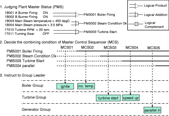

  

  Example of duty supervisor role description

  Fig. 14.5

  

  Example of group leader’s role description

In the first part of Fig. 14.4, an exemplified logic diagram is shown, which is used to identify plant master status (PMS) with the measured sensor values. In the second part of Fig. 14.4, master control sequencers (MCS), which are produced by the result of logical additions of one or more PMS values, are shown. For example, MCS05 is produced by the result of logical addition of PMS001, PMS002, and PMS003. In the third part of Fig. 14.4, the activities to be triggered by the respective MCS are shown.

Each activity enclosed in a shaded box is initiated by the respective MCS. These activities are conducted by the group leaders and operators.

The refinement of activity “turbine start,” defined in Fig. 14.4, is illustrated in Fig. 14.5. In the first part of Fig. 14.5, it is shown that MSD101, the logical product of 1T020, and 1T021, which are logical variables, triggers MSD101. In the second part of Fig. 14.5, the “IF-THEN rule” that triggers OPERATION or PRECONDITION BAD is illustrated. Each OPERATION is controlled by the shown logical expression on the logical variables: TANS, CANS, and PANS (TANS corresponds to trigger condition, CANS to post-condition, and PANS to precondition). As shown in Fig. 14.5, OPERATION is refined into atomic actions: WORKER, MESSAGE, VOICE ANNOUNCE, and LAMP. PRECONDITION BAD is refined into several individual messages.

Using the duty supervisor role descriptions and group leader role descriptions shown in Figs. 14.4 and 14.5, how to classify invariants from variants are analyzed. The results of the analysis are summarized as follows:

• 1. Invariants

  • (a) The semantics of the EPG-SPL framework, which is described in Sect. 5

  • (b) The logical expression to define conditions for controlling every activities

  • (c) The operational semantics for APSS called SCIA, which is described in Sect. 4

• 2. Variants

  • (a) The expressions used to identify variables in PMS, MCS, MSD, and OB

  • (b) The measured values to be used in the conditions defined in the logical expressions

  • (c) The expressions used to identify actions

  • (d) The expressions used to identify messages

Each set of role descriptions is transformed to each table respectively in the way as described below:

• (a) The role descriptions of the duty supervisor shown in Fig. 14.4 are transformed to the table called Master Control Status (MCS) and Plant Master Status (PMS).

• (b) The role descriptions of group leader shown in Fig. 14.5 are transformed to the table called Operation Block (OB) and Multicondition Status Determiner (MSD).

• (c) The role descriptions of operator, not shown in the Figs. 14.4 and 14.5, are transformed to the table called Worker Control Driver (WCD).

4 APSS Framework

Status, Condition, Interaction, and Control (SCIA) is an operational semantics that satisfies the execution of the component-based software architecture called APSS framework shown in Fig. 14.11. The APSS framework allows building hierarchically structured program components for implementing APSS systems. In SCIA, the execution of every atomic component is concurrent and their coordination is expressed in terms of event-oriented architecture.

• Status is the state that is common to all plant start-up operations such as “Start Preparation,” “Condense Water Clean-up,” “Low Pressure Heater Clean-up,” “High Pressure Heater Clean-up,” “Ignition Preparation,” “Boiler Ignition,” “Turbine Start-up,” “Synchronization,” and “Increase Power.”

• Condition is the logical variable defined by a logical expression that consists of logical variables called events and logical operators. Logical composition of atomic events, each of which denotes a deviation of input value from some threshold values.

• Event is defined by interaction involves plant status, events, conditions, and controls, and defines rules to activate or deactivate controls using logical expressions that comprise status events and conditions.

• Control presents logical expressions to define preconditions, trigger conditions, trap condition, and post-conditions that used to control corresponding actions.

Figure 14.6. illustrates an example of temporal relationship between status, trap condition, trigger condition, precondition, post-condition, and control.

Fig. 14.6

Timing chart [3]

Table 14.1 illustrates an example of the semantic relationships between conditions, variables, rules, and controls. The controller Cont.1521 can be activated or deactivated by the result of logical conjunction between condition Cond.0311 and Cond.0312, shown in Table 14.1. The activities to be performed by Cont.1521 are defined in Table 14.2.

Table 14.1 Conditions for controller initiation

Table 14.2 Definition of controller activities

DSL-EPG for the APSS system consists of the six kinds of fill-in-the-blank formats, which are Plant Master Status (PMS), Multicondition Status Determiner (MSD), Master Control Sequencer (MCS), Alarm Group (ALG), Operation Block (OB), and Auxiliary Tables.

• 1. DSL-PMS: DSL for defining Plant Master Status (an example is shown in Fig. 14.7): the logical tables to specify plant master status and to set system flags such as boiler ignition, turbine start-up, synchronization, etc.

  Fig. 14.7

  

  DSL-PMS

• 2. DSL-MCS: DSL for defining Master Control Sequencer (an example is shown in Fig. 14.8): the decision tables that specify parameters that are used to choose control sequence codes.

  Fig. 14.8

  

  DSL-MCS

• 3. DSL-MSD: DSL for defining Multicondition Status Determiner (an example is shown in Fig. 14.9): the logical tables that specify parameters used to select processes to be activated.

  Fig. 14.9

  

  DSL-MSD

• 4. DSL-ALG: DSL for defining Alarm Group definition: the logical tables that specify alarming devices and how to drive those devices.

• 5. DSL-OB: DSL for defining Operation Block (an example is shown in Fig. 14.10): the logical tables that are used to select the objective WCD and to specify preconditions, post-conditions, and logical expressions.

  Fig. 14.10

  

  DSL-OB

• 6. Auxiliary Table:

  • (a) I–O List: Input–Output List

  • (b) WCD: DSL for defining control of worker drivers

Inside the APSS framework, seven software components (Process-scheduler, ACP, EAC, BOC, WCP, CIS, and MAS) and three code storages (I/O-code base, plant-code base, and worker-code base), shown in Fig. 14.11, are accommodated. The APSS framework will be included as a constituent of the provisional machine shown in Fig. 14.14.

Fig. 14.11

APSS framework

The roles of those components are as follows:

• Process-scheduler: The role of Process-scheduler (PS) is the mediation between other six framework components and the operating system. PS schedules, monitors, and controls processes to drive processes called ACP, EAC, BOC, WCP, CIS, and MAS.

• Contact Input Scan (CIS): Driven periodically by PS, CIS scans states of switch contacts using the data provided by I/O-code base. Whenever any event (deviation from the defined range or condition) is found, CIS sends action to EAC.

• Multiple Analog Scan (MAS): Driven periodically by PS, MAS scans states of analog inputs using the data provided by I/O-code base. Whenever any event (deviation from the defined range or condition) is found, MAS sends action to EAC.

• Executive Action Control (EAC): EAC is activated periodically in the highest priority, and receives actions sent from CIS and MAS. Accordingly, EAC transfers to ACP, the names of the occurred actions and the identification numbers of OB tables (OB assignment) that are related with the actions.

• Activity Control Processor (ACP): Driven by the messages from EAC, ACP takes the codes of the assigned OB tables from the plant-code base and interprets. As the result of interpretation, WCP or BCO is activated.

• Worker Control Processor (WCP): This is the process to drive various external devices such as relays, switches, servo motors, or valve controllers. WCD interprets the codes in the worker-code base and plant-code base assigned by ACP and sends outputs to control external devices.

• Blocking Conditioning Output (BCO): This is the process to select and block some outputs for the purposes of protection by interpreting the assigned conditions from the I/O-code base and plant-code base.

In order to verify the function of APSS software, Toshiba has developed the testing software environment shown in Fig. 14.12. The testing software environment implements the following subfunctions:

Fig. 14.12

Testing environment for APSS codes generated from DSL-EPG

• Plant input SIMulation Program System (SIMPS): The function to apply time sequential data to each input of APSS software.

• Output Value Monitor: The function to enable monitoring each output of APSS software by using graphical method.

• Data Feedback Simulator: The function to simulate the feedback from output data to input of APSS system based on the combination of software code. This function is applied to verify the functions of some important part of the plant such as main turbine.

These functions effectively work for verifying the APSS software functions, for example, validity of data provided I/O-code base, activities, controlled by plant-code base and process driven by worker-code base.

5 Software Product Line

5.1 Product Line Scoping Supports Business Strategy [7]

The scoping [4, 5] of EPG-SPL has been decided based on the Toshiba Corporation’s business strategy that defines market segments in the EPG world. The market segments covered by the EPG-SPL are fossil fuel fired (coal fired, oil fired, or liquefied natural gas fired) steam cycle, steam/gas combined-cycle and nuclear power plants (e.g., boiling-water type) to be provided by public utility companies, as well as by private companies. The EPG-SPL scope also includes other parameters such as listed as follows:

• 1. Type of software platform

• 2. Type of EPG middleware

• 3. Type of DSL-EPG interpreter

• 4. Various specialties that are required depending on each market segment

• 5. Various specialties that are derived from the properties of customers, plant-equipment manufacturers, and type of plant/control devices

• 6. Type of functionalities covered by the EPG-SPL

The functionalities covered by the EPG-SPL are plant-monitoring, plant-performance calculation, APSS, man–machine interactions, plant-operational graphics display. The EPG-SPL constituents are classified in accordance with those EPG-SPL functionalities. It means that APSS is one of the EPG-SPL constituents, and the operational semantics SCIA, described in Sect. 4, is the semantics that specifically supports only APSS.

The model of EPG-SPL-code configuration is shown in Fig. 14.13. It comprises four major parts: DSL-EPG-code generator, code based for the defined four market segments, functional programs for DSL-EPG interpreter and specialties used for the particular functionalities, and EPG middleware.

Fig 14.13

Model of code configuration of the EPG-SPL

5.2 Architecture of EPG-SPL [8]

The architecture of EPG-SPL and how to use it is modeled in Fig. 14.14. The invariants described in Sect. 3.2, e.g., the operational semantics (SCIA) for APSS, commonly used logical expressions, and event-driven architecture, are classified in accordance with the market segments and associated parameters, explained in Sect. 5.1., and mounted on the repository described in the left edge of Fig. 14.14 through Meta Class format sheets. The variants described in Sect. 3.2, which are variables in PMS, MCS, MSD, and OB, variables to identify actions, and variables to identify messages, are input to the code generators through the DSL documents shown in the top right corner of Fig. 14.14.

Fig. 14.14

Architecture of EPG software product line

In case that we need to construct a whole set of codes to be released to a target power plant, the plant-specific invariants defined by the meta-classes, described using the Meta Class format sheets shown in the left-top part of Fig. 14.14, are put into the EPG-SPL by the developers. The task called “configuration,” shown in Fig. 14.14, selects the necessary sets of invariants, defined in the Meta Class format sheets, from the repository, and put those invariant sets into the provisional machine automatically. The provisional machine consists of code bases, interpreters, EPG software framework core, platform and hardware. The interpreters can be made to execute using all the defined variants and invariants using EPG middleware, platform, and hardware, on the provisional machine. The codes system mounted on the provisional machine can be tested using plant input SIMulation Program System (SIMPS) by the human task “testing”.

In case that the codes released and deployed in the target plant should be changed as results of maintenance, improvement or enhancement, contents of the repository will be updated accordingly in order to match with the deployed codes through human tasks “testing,” “fixing,” and “revision.” The fact that any revision has been made will be announced to other plants by the human task “distribution.” When any new invariant features are developed, those invariants can be uploaded to the repository through human task “registration.”

6 Cost and Benefits

In order to manage and control cost and benefits during the development and adoption of EPG-SPL, a guideline was developed [1, 2]. The guideline consists of three kinds of tables shown in Tables 14.3, 14.4, and 14.5, namely ROI calculation form, variable cost table, and fix cost table. Using this guideline, cost and benefits are controlled so that shortage of return, to be entered in the bottom row of Table 14.3, should never get into the red in each fiscal year.

Table 14.3 ROI calculation form

Table 14.4 Calculation of variable cost

Table 14.5 Calculation of fixed cost

The ordinal numbers shown in the top of every table identify the sequential order of the fiscal years in the adoption stage. Usually, the corporate level of the company defines the values such as standard interest rate (cost of capital), the tax rate, and the depreciation. The number of shipments in fiscal year i, or n(i), means the number of systems released and installed within this fiscal year, developed by the adoption of EPG-SPL. The sales amount S(i) means the sum of customer’s payment within fiscal year i.

The breakdowns of “variable cost” and “fixed cost” are listed respectively in Tables 14.4 and 14.5. The explanations for every symbolized item are noted in the rightmost columns.

In Table 14.4, the cost of maintenance, enhancement, and configuration management required for running installed systems should be included in team cost TC(i).

The costs of activities, such as development of new items necessary to satisfy individual customer’s requirements, development of additional assets, improvement of the existing assets, and the development of sub-domain product lines, modification efforts (such as development of sub-domain EPG-SPL, and modification of EPG-SPL adoption programs) should also be included in TC(i).

In Table 14.5, the organizational costs necessary for keeping the fixed activities and tasks, such as the ones conducted by the fixed organizational elements should be included in department expense DX(i).

Using VC(i) and FC(i) calculated in Tables 14.4 and 14.5, the shortage of the return SR(i) should be calculated using the equation in the bottom row of Table 14.3. This value suggests the residual return that should be recovered by the cash flows in the residual years.

The guide addresses the following processes:

• 1. Time scale: The length of EPG-SPL life and the time span necessary for conducting each stage should be estimated at the beginning of or in the early stage of development. At every fiscal year in the adoption stage, its ordinal number starting from the first year should be identified and entered in the row #1 of the tables.

• 2. PV calculation: The expected cash flows which could be obtained at every fiscal year in the adoptions stage should be predicted at the end of development stage at the row #19 of Table 14.3. And NPV (accumulation of the PVs) should be calculated and used for getting SR(i) at the row #20 of Table 14.3.

• 3. Cost control in adoption stage: The cost limit for conducting adoption stage could be determined using the calculated SR(i) described in item (2), so that the cost limit should not exceed the NPV. The adoption stage should be managed and controlled so that the actual cost should be less than the cost limit.

• 4. Renewal of SPL generation: If it becomes clear that the shortage of return will not to be recovered within the predetermined EPG-SPL lifetime, EPG-SPL adoption plan should be modified and improved totally. In our case, such an overall improvement was made in 1982, 1988, 1993, and 1996, as is described by Matsumoto 2007 [2].

7 Conclusion

In this chapter, major features of APSS system and the software family, including DSL-EPG, its processor and EPG-SPL, which supports automatic code generation for each APSS application, are introduced. The sets of rules for operating the plant, where each rule defines a relationship between plant status, events, conditions, and operator’s actions, are defined in the collaborative work participated by customers, plant operators, and APSS developers. The variants included in each rules can be specified, and described with using DSL-EPG. The DSL-EPG processor analyzes those descriptions to generate application codes [9]. The paper also illustrates how EPG-SPL, which comprises APSS, is structured and maintained from the viewpoint of cost and benefit.

The text of this paper was mostly produced by the third author, one of the original creators of the system covered by this paper, and was compiled with the figures, tables and references by the first and second authors.

References

Matsumoto, Y.: Management and financial controls of a software product line adoption. In: Kang, K.C., et al. (eds.) Applied Software Product Line Engineering, pp. 399–419. CRC Press, Taylor Francis Group, Boca Raton, FL. 33497–2742 (2009)
Matsumoto, Y.: A guide for management and financial controls of product lines. In: Proceedings of IEEE 11th International Software Product Line Conference, pp. 163–170 (2007)
Matsumoto, Y.: A method of software requirements definition in process control. In: Proceedings of COMPSAC77, pp. 128–132 (1977)
Clements, P., Northrop, L.: Software Product Lines: Practices and Patterns. Addison-Wesley, Reading, MA (2002)
Czarnecki, K., Eisennecker, U.W.: Generative Programming: Methods, Tools, and Applications. Addison-Wesley, New York (2000)
IEEE Std 828-1988, IEEE Standard for Software Configuration Management Plans. Software Engineering Standards Committee of the IEEE Computer Society (1998)
ISO/IEC DIS 26551, Software and systems engineering – Tools and methods for product line requirements engineering. International Organization for Standardization/International Electrotechnical Commission (2012)
ISO/IEC DIS 26555, Software and systems engineering – Tools and methods for product line technical management. International Organization for Standardization/International Electrotechnical Commission (2012)
Matsumoto, Y.: Mapping Dynamic Software Product Line Properties to the Current Toshiba Software Product Line for Electric Power Generation, http://www5d.biglobe.ne.jp/~y-h-m/Mapping_DSPL_Properties.pdf
Author information
Authors and Affiliations
Corresponding author
Editor information
Editors and Affiliations
Rights and permissions
Copyright information
© 2013 Springer-Verlag Berlin Heidelberg
About this chapter
Cite this chapter
Okamoto, M., Fujii, M., Matsumoto, Y. (2013). Variability in Power Plant Control Software. In: Capilla, R., Bosch, J., Kang, KC. (eds) Systems and Software Variability Management. Springer, Berlin, Heidelberg. https://doi.org/10.1007/978-3-642-36583-6_14
Download citation
DOI: https://doi.org/10.1007/978-3-642-36583-6_14
Published:
Publisher Name: Springer, Berlin, Heidelberg
Print ISBN: 978-3-642-36582-9
Online ISBN: 978-3-642-36583-6
eBook Packages: Computer ScienceComputer Science (R0)