Proof Nets as Formal Feynman Diagrams

Abstract

The introduction of linear logic and its associated proof theory has revolutionized many semantical investigations, for example, the search for fully-abstract models of PCF and the analysis of optimal reduction strategies for lambda calculi. In the present paper we show how proof nets, a graph-theoretic syntax for linear logic proofs, can be interpreted as operators in a simple calculus.

This calculus was inspired by Feynman diagrams in quantum field theory and is accordingly called the φ-calculus. The ingredients are formal integrals, formal power series, a derivative-like construct and analogues of the Dirac delta function.

Many of the manipulations of proof nets can be understood as manipulations of formulas reminiscent of a beginning calculus course. In particular, the “box” construct behaves like an exponential and the nesting of boxes phenomenon is the analogue of an exponentiated derivative formula. We show that the equations for the multiplicative-exponential fragment of linear logic hold.

These keywords were added by machine and not by the authors. This process is experimental and the keywords may be updated as the learning algorithm improves.

1 Introduction

Girard’s geometry of interaction programme [Gir89a, Gir89b, Gir95a] gave shape to the idea that computation is a branch of dynamical systems. The point is to give a mathematical theory of the dynamics of computation and not just a static description of the results as in denotational semantics.

The key intuition is that a proof net, a graphical representation of a proof, is decorated with operators at the nodes which direct the flow of information through the net. Now the process of normalization is not just described by a syntactic rewriting of the net, as is usually done in proof theory, but by the action of these operators. The operators are interpreted as linear operators on a suitable Hilbert space. In this framework normalizability corresponds to nilpotence of a suitable operator. Given the correspondence between proof nets and the λ-calculus, a significant shift has occurred. One now has a local, asynchronous algorithm for β-reduction [DR93, ADLR94]. Abramsky and Jagadeesan [AJ94b] presented geometry of interaction using dataflow nets using fixed point theory instead of the apparatus of Hilbert spaces and operators. However, the information flow paradigm is clear in both presentations of the geometry of interaction.

In the present paper we begin an investigation into the notion of information flow. Our starting point is the notion of Feynman diagram in Quantum Field Theory [Fey49b, Fey49a, Fey62, IZ80]. These are graphical structures which can be seen as visualizations of interactions between elementary particles. The particles travel along the edges of the graph and interact at the vertices. Associated with these graphs are integrals whose values are related to the observable scattering processes. This intuitive picture can be justified from formal quantum field theory [Dys49]. Mathematically quantum field theory is about operators acting on Hilbert spaces, which describe the flow of particles. One can seek a formal analogy then with the framework of quantum field theory and the normalization process as described by the geometry of interaction.

We have, however, not yet reached a full understanding of the geometry of interaction. We have, instead, made a correspondence between proof nets and terms in a formal calculus, the φ-calculus, which closely mimics some of the ideas of quantum field theory. In particular we have imitated some of the techniques, called “functional methods” in the quantum field theory literature [IZ80], and shown how to represent the exponential types in linear logic as an exponential power series. The manipulations of boxes in linear logic amounts to certain simple exponential identities. Thus we have more than a pictorial correspondence; we have formal integrals whose evaluation corresponds to normalization.

This work was originally presented at the Newton Institute Semantics of Computation Seminar in December 1995. The publication of this edition provided an excellent opportunity to revive the work. We thank Bob Coecke for giving us the opportunity to do so.

1.1 Functional Integrals in Quantum Field Theory

Before we describe the φ-calculus in detail we will sketch the theory of functional integrals as they are used in quantum field theory. This section should be skipped by physicists. This section is very sketchy, but, it is hoped, it will provide an overview of the method of functional integrals and, more importantly, it will give a context for the φ-calculus to be introduced in the next section. It has been our experience that computer scientists, categorists and logicians, who have typically never heard of functional integrals tend to view the φ-calculus as an ad-hoc formalism “engineered” to capture the combinatorics of proof nets. In fact, almost everything that we introduce has an echo in quantum field theory.

There are numerous sources for functional integrals. The idea originated in Feynman’s doctoral dissertation [Bro05] published in 1942, now available as a book. The basic idea is simple. Usually in nonrelativistic quantum mechanics one associates a wave function $\psi(\boldsymbol{x},t)$ which obeys a partial differential equation govening its time evolution, the Schrödinger equation. The physical interpretation is that the probability density of finding the particle at location $\boldsymbol{x}$ at time t is given by $|\psi(\boldsymbol{x},t)|^2$. The wave function describes how the particle is “smeared out” over space; it is called a probability amplitude function.

In the path integral approach, instead of associating a wave function with a particle one looks at all possible trajectories of the particle – whether dynamically possible or not according to classical mechanics – and associates a probability amplitude with each trajectory. Then one sums over all paths to obtain the overall probability amplitude function. This requires making sense of the “sum over all paths.” It is well known that the naive integration theory cannot be used, since there are no nontrivial translation-invariant measures on infinite-dimensional spaces, like the space of all paths. However, Feynman made skillful use of approximation arguments and showed how one could calculate many quantities of interest in quantum mechanics [FH65]. Furthermore, this way of thinking inspired his later work on quantum electrodynamics [Fey49b, Fey49a]. Since then the theory of path integrals has been placed on a firm mathematical footing [GJ81, Sch81, Sim05].¹

The functional integral is the extension of the path intgeral to infinite-dimensional systems. Moving to infinite dimensional systems raises the mathematical stakes considerably and led to much controversy about whether this is actually well-defined. In the past two decades a rigourous theory, due to Cartier and DeWitt-Morette has appeared [CDM95] but not everyone accepts that this formalises what physicists actually do when they make field-theoretic calculations.

What physicists do is to use a set of rules that make intuitive sense and which are guided by analogy with the ordinary calculus. Some of the ingredients of this formal calculus are entirely rigourous, for example, the variational derivative [GJ81]; but the existence of the integrals remains troublesome.

In classical field theory one has a function, say φ defined on the spacetime M. This function may be real or complex valued, and in addition, it may be vector or tensor or spinor valued. Let us consider for simplicity a real-valued function; this is called a scalar field. Thw field obeys a dynamical equation, for example the scalar field may obey an equation like $\Box\phi + m^2\phi=0$ where □ is the four-dimensional laplacian.

In quantum field theory, the field is replaced by an operator acting on a Hilbert space of states. The quantum field is required to obey certain algebraic properties that capture aspects of causality, positivity of energy and relativistic invariance. The Hilbert space is usually required to have a special structure to accomodate the possibility of multiple particles. There is a distinguished state called the vacuum and one can vary the number of particles present by applying what are called creation and annihilation operators. There is a close relation between these operators and the field operator: the field operator is required to be a sum of a creation and an annihilation operator.

The main idea of the functional integral approach is that the fundamental quantities of interest are transition amplitudes between states. These are usually states of a quantum field theory and are often given in terms of how many particles of each type and momentum are present in the field: this description of the states of a quantum field is called the Fock representation. The most important quantity is the vacuum-to-vacuum transition amplitude, written ${\langle {0,-} \mid {0,+}\rangle}$, where ${{\langle {0,-}\mid}}$ represents the vacuum at early times and ${{\mid {0,+}\rangle}}$ is the late vacuum. The idea of the functional approach is this can be obtained by summing a certain quantity—the action—over all field configurations interpolating between the initial and the final field.

This can be written as

$$W = \int [d\phi]\exp{[-\int d^3\boldsymbol{x} \left(\frac12 \phi{{\cal D}}\phi\right)]}$$

where ${{\cal D}}$ is some differential operator coming from the classical free field theory. The $[d\phi]$ is supposed to be the measure over all field configurations. Though we do not define it, we can do formal manipulations of this functional. In order to extract interesting results, we want not just the vacuum-to-vacuum trnasition probabilities but the expectation values for products of field operators, e.g. ${{\langle {0} \mid {\phi(x)\phi(y)}\mid {0}\rangle}}$ and other such combinations. In order to do this we add a “probe” to the field which couples to the field and which can be varied. This is fictitious, of course, and will be set to zero at the end. The probe (usually called a current) is typically written as $J(x)$. The form we now get for W is

$$W[J] = \int [d\phi]\exp{[-\int d^3\boldsymbol{x} \left(\frac12 \phi{{\cal D}}\phi\right) -J\phi]}.$$

Note that W is now a functional of J.

Before we can do any calculations we need to rewrite the term. Consider, for the moment ordinary many-variable calculus. Suppose we write $(,\!)$ for the inner product on $\mathbb{R}^n$ we can write a form

$$Q(x) = \frac12 (x,Ax) + (b,x) .$$

Now recall the gaussian integral in many variables is just

$$\int d^nx \exp{-\frac12(x,Ax)} = [det(A)^{-\frac12}]$$

where A is an ordinary $n\times n$ matrix with positive eigenvalues and we have ignored factors involving 2π. To deal with Q we complete the square by setting $y = A^{-1}b$ and get

$$Q(y) + \frac12 (x-y,A(x-y)) = Q(x).$$

Using this and changing variables appropriately, we get

$$\int d^nx \exp{-Q(x)} = [\textit{det} A]^{-\frac12}\exp{-Q(y)}.$$

Now in the functional case, the determinant of an operator does not make sense naively, we will just ignore it here. In actual practice these divergent determinants are made finite by a process called regularization and dealt with. It should be noted that there is a fascinating mathematical theory of these determinants that we will not pursue here.

Returning to our functional expression we get

$$W[J] = \exp{\frac12 \int d^4 x d^y J(x) {{\cal D}}^{-1} J(y)}.$$

How are we to make sense of the inverse of a differential operator? It is well-known in mathematics and physics as the Green’s function.² It is well-defined as a distribution. In quantum field theory, the Green’s function with appropriately chosen boundary conditions is called the Feynman propagator.

In order to obtain interesting quantities we “differentiate” $W[J]$ with respect to the function $J(x)$. This is called the variational derivative and is well defined, see, for example, [GJ81]. Roughly speaking, one should think of this as a directional derivative in function space. The definition given in [GJ81] (page 202) is

$$(D_{\psi}(A))(\phi) = \lim_{\epsilon\rightarrow 0} [A(\phi +\epsilon\psi) - A(\phi)]/\epsilon.$$

This is the derivative of the functional A of φ in the direction of the function φ. Now we can consider the special case where ψ is the Dirac delta “function” $\delta(x)$ and write is using the common notation as

$$\frac{\delta}{\delta\phi(x)} A(\phi) \equiv D_{\delta(x)} A(\phi).$$

A very useful formula is

$$\frac{\delta}{\delta\phi(x)} \phi(y) = \delta(x,y).$$

Please note that some of the deltas are part of the variational derivative and some are Dirac distributions: unfortunate, but this is the common convention.

How do we use these variational derivatives? If we consider the form of $W[J]$ before we rewrote it in terms of propagators we see that a variational derivative with respect to J brings down a factor of φ and thus, if we do this twice, for example, gives us ${{\langle {0} \mid {\phi(x_1)\phi(x_2)}\mid {0}\rangle}}$. If we look at the trnasformed version of W the same derivatives tell us how to compte this quantity in terms of propagators. So in the end one gets explicit rules for calculating quantities of interest.

For a given field theory, the set of rules are called the Feynman rules and give explicit calculational prescriptions. The functional integral formalism is used to derive these rules. The rules can also be obtained more rigourously from the Hamiltonian form of the field theory as was shown by Dyson [Dys49]. All this can be made much more rigourous. The point is to show some of the calculational devices that physicists use. It is not be expected that after reading this section one will be able to calculate scattering cross-sections in quantum electrodynamics. The point is to the see that the φ-calculus is closely based on the formalisms commonly in use in quantum field theory.

1.2 Linear Realizability Algebra

This section is a summary of the theory of linear realizability algebras as developed by Abramsky [Abr91]. The presentation here closely follows that of Abramsky and Jagadeesan [AJ94a]. The basic idea is to take proofs in linear logic in sequent form and to interpret them as processes. The first step is to introduce locations; which one can think of as places through which information flows in or out of a proof. Of course the diagrammatic form of proof nets carry all this information without, in Girard’s phrase “the bureaucracy of syntax”. However, to make contact with an algebraic notation we have to reintroduce the locations to indicate how things are connected. In process terms these will correspond to ports or channels or names as in the π-calculus [Mil89]. In our formal calculus, locations will be introduced with roughly the same status. The set of locations $\mathcal{L}$ is ranged over by x,y,z,….

The next important idea is that of located sequents, of the form

$$\vdash x_1 : A_1, \ldots, x_k: A_k$$

where the x _i are distinct locations, and the A _i are formulas of $\texttt{CLL}_2$. These sequents are to understood as unordered, i.e. as functions from $\{ x_1,\ldots, x_k \}$- the sort of the sequent- to the set of $\texttt{CLL}_2$ formulae.

A syntax of terms (Fig. 7.3) is introduced , which will be used as realizers for sequent proofs in $\texttt{CLL}_2$. The symbols P,Q,R are used to range over these terms, and write $\texttt{FN}(P)$ for the set of names occurring freely in P—its sort. With each term-forming operation one gives a linearity constraint on how it can be applied, and specifies its sort. In the very last case, the so-called “of course” modality, we have imposed a restriction that if a location is introduced by an “of course” we will require that all the other variables have been previously introduced by either derelictions, weakenings or contractions. We are interested in terms that arise from proof nets so we think of our terms as being typed; this is a major difference between our LRAs and those introduced by Abramsky and Jagadeesan [AJ94b].

Fig 7.1

Syntax: linear realizability algebra

There is an evident notion of renaming $P[x/y]$ and of α-conversion $P \equiv_{\alpha} Q$.

Terms are assigned to sequent proofs in $\texttt{CLL}_2$ as in Fig. 7.3.

The rewrite rules for terms, corresponding to cut-elimination of sequent proofs, can now be given. This is factored into two parts, in the style of [BB90]: a structural congruence ≡ and a reduction relation →.

The structural congruence is the least congruence ≡ on terms such that:

• (SC1) $P \equiv_{x} Q {{\Rightarrow}} P \equiv Q$

• (SC2) $P {{\cdot_{x}}} Q \equiv Q {{\cdot_{x}}} P$

• (SC3) $\omega(P_1,\ldots ,P_k) \equiv \omega(P_1,\ldots, P_i {{\cdot_{x}}} Q, \ldots ,P_k)$, if $x \in \texttt{FN}(P_i)$.

The reductions are as follows:

• .

• (R7)   $W_{z}(P) {{\cdot_{z}}} {{\textbf{\,!\,}}}^{x}_{z}(Q) {{ \rightarrow }} W_{\boldsymbol{x}}(P)$, where $\texttt{FN}(Q) \setminus \{ x \} = \boldsymbol{x}$.

• (R8)   $C^{z',z''}_{z}(P) {{\cdot_{z}}} {{\textbf{\,!\,}}}^{x}_{z}(Q) {{ \rightarrow }} C^{\boldsymbol{x'},\boldsymbol{x''}}_{\boldsymbol{x}} (P {{\cdot_{z'}}} {{\textbf{\,!\,}}}^{x}_{z'}(Q[\boldsymbol{x'} /\boldsymbol{x}]) {{\cdot_{z''}}} {{\textbf{\,!\,}}}^{x}_{z''}(Q[\boldsymbol{x''} /\boldsymbol{x}]))$, where $\texttt{ FN}(Q) \setminus \{ x \} = \boldsymbol{x}$.

• (R9)   ${{\textbf{\,!\,}}}^{x}_{z}(P) {{\cdot_{u}}} {{\textbf{\,!\,}}}^{v}_{u}(Q) {{ \rightarrow }} {{\textbf{\,!\,}}}^{x}_{z}(P {{\cdot_{u}}} {{\textbf{\,!\,}}}^{v}_{u}(Q))$, if $u \in \texttt{FN}(P)$.

Fig 7.2

Realizability semantics

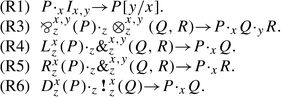
We are using the same numbering as in [AJ94b] and have left out R2, which talks about units. We write bold face to stand for sequences of variables.

These reductions can be applied in any context.

$${{ \frac{{{P {{ \rightarrow }} Q}}}{{{C[P] {{ \rightarrow }} C[Q]}}}}}$$

and are performed modulo structural congruence.

$${{ \frac{{{P' \equiv P \;\;\; P {{ \rightarrow }} Q \;\;\; Q' \equiv Q }}}{{{P {{ \rightarrow }} Q}}}}}$$

The basic theorem is that this algebra models cut elimination is classical linear logic. The precise statement is

Proposition 7.3.1

[Abramsky] Let Π be a sequent proof of ⊢Γ in $\texttt{CLL}_2$ with corresponding realizing term P. If $P {{ \rightarrow }} Q$, with Q cut-free (i.e. no occurrences of ${{\cdot_{\alpha}}}$), then Π reduces under cut-elimination to a cut-free sequent proof Π‣ with corresponding realizing term Q.

In order to verify that one correctly models the process of cut-elimination in linear logic it suffices to verify the LRA equations R1 through R9. In fact we will also check the following equation:

$${{\&}}^{x,y}_{z}(P,Q) {{\cdot_{u}}} R {{ \rightarrow }} {{\&}}^{x,y}_{z}(P {{\cdot_{u}}} R ,Q {{\cdot_{u}}} R ) \; [u \in \texttt{ FN}(P) \cap \!\texttt{ FN}(Q)]$$

This is the commutative with-reduction and is not satisfied in the extant examples of LRA.

1.3 The φ-Calculus

In this section we spell out the rules of our formal calculus. Briefly the ingredients are

• Locations:   which play the same role as the locations in the located sequents of LRA.

• Basic terms:   which, for the multiplicative fragment, play the role of LRA terms.

• Operators:   Which act on basic terms and which play the role of terms in the full LRA.

In order to define the basic terms we need locations, formal distributions, formal integrals and simple rules obeyed by these. In order to define operators we need to introduce a formal analogue of the variational derivative. This variational derivative construct is very closely modelled on the derivation of Feynman diagrams from a generating functional.

We assume that we are modelling a typed linear realizability algebra with given propositional atoms. We first formalize locations. We assume further that axiom links are only introduced for basic propositional atoms. We use the phrases “basic types” and “basic propositional atoms” interchangeably.

Definition 1

We assume that there are countably many distinct symbols, called locations for each basic type. We assume that there are the following operations on locations: if x and y are locations of types A and B respectively, then $\langle x,y \rangle$ and $[x,y]$ are locations of type $A{\otimes} B$ and respectively. We use the usual sequent notation $x: A,y: B\vdash \langle x,y\rangle : A{\otimes} B$ and to express this.

Now we define expressions.

Definition 2

The collection of expressions is given by the following inductive definition. We also define, at the same time, the notion of the sort of an expression, which is the set of free locations, and their types, that appear in the expression.

• 1. Any real number r is an expression of sort ∅.

• 2. Given any two distinct locations, $x: A$ and $y: A^{\perp} \delta(x,y)$ is an expression of sort $\{x: A,y: A^{\perp}\}$.

• 3. Given any two expressions P and Q, PQ and $P + Q$ are expressions of sort $\mathsf{S}(P)\cup \mathsf{S}(Q)$.

• 4. Given any expression P and any location $x: A$ in P, the expression $\int P dx$ is an expression of sort $\mathsf{S}(P)\setminus\{x: A\}$.

The expressions above look like the familiar expressions that one manipulates in calculus. The sorts describe the free locations that occur in expressions. The integral symbol is the only binding operator and is purely formal. Indeed any suitable notation for a binder will do, a more neutral one might be something like $Tr(e,x)$, which is more suggestive of a trace operation.

The equations obeyed by these expressions mirror the familiar rules of calculus. The only exotic ingredients are that the δ behaves like a Dirac delta “function”. We will actually present a rewrite system rather than an equational system but one can think of these as equations.

We use the familiar notation $P(\ldots,y/x,\ldots)$ to mean the expression obtained by replacing all free occurrences of x by y with appropriate renaming of bound variables as needed to avoid capture; x and y must be of the same type of course. We now define equations that the terms obey.

Definition 3

• 1. $\delta(x,y) = \delta(y,x)$

• 2. $\int (\int P dx) dy = \int (\int P dy) dx$

• 3. $(P+Q)+R=P+(Q+R)$

• 4. $(P + Q) = (Q + P)$

• 5. $P\cdot (Q\cdot R)=(P\cdot Q)\cdot R$

• 6. $P\cdot Q = Q\cdot P$

• 7. $P\cdot (Q_1+Q_2)=P\cdot Q_1+P\cdot Q_2$

• 8. $P+0= P$.

• 9. $P\cdot 1= P$.

• 10. $P\cdot 0= 0$.

• 11. $\int P(\ldots,x,\ldots)\delta(x,y) dx = P(\ldots,y/x,\ldots)$.

• 12. $\delta([x,y],\langle u,v\rangle) = \delta(x,u)\delta(y,v)$.

• 13. If $P= P'$ then $PQ= P'Q$.

• 14. If $P= P'$ then $P+Q= P'+Q$.

• 15. If $P= P'$ then $\int P dx = \int P' dx$.

These equations are very straightforward and can be viewed as basic properties of functions and integration or about matrices and matrix multiplication. The only point is that with ordinary functions one cannot obtain anything with the behaviour of the δ-function; these are, however, easy to model with distributions or measures.

In order to model the exponentials and additives we need a rather more elaborate calculus. We introduce operators which are inspired by the use of generating functionals for Feynman diagrams in quantum field theory [IZ80, Ram81]. The two ingredients are formal power series and variational derivatives. In order to model pure linear logic the formal power series that arise as power-series expansions of exponentials are the only ones that are needed. We introduce a formal analogue of the variational derivative operator, commonly used in both classical and quantum field theories [Ram81]. For us the variational derivative plays the role of a mechanism that extracts a term from an exponential.

As before we have locations and expressions. We first introduce a new expression constructor.

Definition 4

If x is a location of type A then $\alpha_A(x)$ is an expression of sort $\{ x:A\}$.

The point of α is to provide a “probe”, which can be detected as needed. For each type and location there is a different α. We will usually not indicate the type subscript on the αs unless they are necessary. The last ingredient that we need in the world of expressions is an expression that plays the role of a “discarder”, used, of course, for weakening.

Definition 5

If x is a location of type $\{ x:A\}$, where A is a multiplicative type, then $W_A(x)$ is an expression of sort $\{ x:A\}$. This satisfies the equations

• 1. $W_{A{\otimes} B}(\langle x,y\rangle) = W_A(x)W_B(y)$,

• 2. .

We can think of $W(x)$ intuitively as “grounding” in the sense of electrical circuits. In effect it provides a socket into which x is plugged but which is in turn connected to nothing else. So it is as if x were “grounded”. If such a $W(x)$ is connected to a wire, $\int W(x)\delta(x,y) dx$ the result will be the same as grounding y. The other two equations express the fact that a complex W can be decomposed into simpler ones. We will introduce another decomposition rule for W after we have described the variational derivatives and a corresponding operator for weakening.

We introduce syntax for operators; these will be defined as maps from expressions to expressions.

Definition 6

Operators are given by the following inductive definition.

• 1. If M is any expression $\hat{M}$ is an operator of the same sort as M.

• 2. If $x:A$ is a location then ${{([{.}]|_{\alpha({x})=0})}}$ is an operator of sort $x:A$.

• 3. If $x:A$ is a location then ${{\frac{\delta}{\delta\alpha({x})}}}$ is an operator of sort $x:A$.

• 4. If P and Q are operators then so are $P+Q$ and $P\circ Q$ their sort is the union of the individual sorts.

• 5. If P is an operator then so is $\int P dx$; its sort is $\mathsf{S}(P)\setminus \{ x\}$.

An operator of sort S acts on an expression of sort S‣ if $S\cap S'$ is not empty.

Operators map expressions to expressions. An important difference between the algebra of expressions and that of operators is that the (commutative) multiplication of expressions has been replaced by the (non-commutative) composition of operators.

The meaning of the operators above is given as follows. We use the meta-variables M,N for expressions and P,Q for operators. We begin with the definition of $\hat{M}$.

Definition 7

$\hat{M}(N) = M\cdot N$.

The notion of composition of operators is the standard one

Definition 8

$[P\circ Q](M) = P(Q(M))$.

Clearly we have $\hat{M}\circ\hat{N} = \hat{MN}$; thus we have an extension of the algebra of expressions. We will write 1 and 0 rather than, for example, $\hat{1}$ to denote the operators. The resulting ambiguity will rarely cause serious confusion.

The next set of rules define the operator ${{([{.}]|_{\alpha({x})=0})}}$. Intuitively this is the operation of “setting $\alpha(x)$ to 0” in an algebraic expression.

Definition 9

If M is an expression then the operator ${{([{.}]|_{\alpha({x})=0})}}$ acts as follows:

• 1. If $\alpha(x)$ does not appear in M then ${{([{M}]|_{\alpha({x})=0})}} = M$.

• 2. ${{([{M N}]|_{\alpha({x})=0})}} = ({{([{M}]|_{\alpha({x})=0})}})({{([{N}]|_{\alpha({x})=0})}})$.

• 3. ${{([{M + N}]|_{\alpha({x})=0})}} = ({{([{M}]|_{\alpha({x})=0})}})+({{([{N}]|_{\alpha({x})=0})}})$.

• 4. ${{([{M\alpha(x)}]|_{\alpha({x})=0})}} = 0$.

The rules for the variational derivative formalize what one would expect from a derivative, most notably the Leibniz rule, rule 5 below.

Definition 10

If M is an expression and x is a location we have the following equations:

• 1. If x and y are distinct locations then ${{\frac{\delta}{\delta\alpha({x})}}}\alpha(y) = 0$.

• 2. If $\alpha(x)$ does not occur in the expression M then ${{\frac{\delta}{\delta\alpha({x})}}}M = 0$.

• 3. ${{\frac{\delta}{\delta\alpha({x})}}}\alpha(x) = 1$.

• 4. ${{\frac{\delta}{\delta\alpha({x})}}}(M+N) = ({{\frac{\delta}{\delta\alpha({x})}}}M)+({{\frac{\delta}{\delta\alpha({x})}}}N)$.

• 5. ${{\frac{\delta}{\delta\alpha({x})}}}(MN) = (M{{\frac{\delta}{\delta\alpha({x})}}}N)+(({{\frac{\delta}{\delta\alpha({x})}}}M)N)$.

Clause 1 is, of course, a special case of clause 2 but is added for emphasis. Intuitively the variational derivative should be viewed as “probing for the presence of α”. The reason that we use these variational derivatives rather than ordinary derivatives is that the dependence on the location is crucial for our purposes. Typically we use the combination of ${{([{.}]|_{\alpha({x})=0})}}$ and ${{\frac{\delta}{\delta\alpha({x})}}}$ so that we are “inserting probes”, “testing for their presence” and then “removing them”. The power of the formalism comes from the interaction between variational derivatives and exponentials.

The remaining rules defining the algebra of operators are given in the next definition.

Definition 11

Operators obey the following equations:

• 1. $\hat{0}(M) = 0$.

• 2. $\hat{1}(M) = M$.

• 3. $(P+Q)(M) = P(M)+Q(M)$.

• 4. $[\int P dx](M) = \int P(M) dx$, where x is not free in M.

One can prove the following easy lemma by structural induction on expressions.

Lemma 7.4.1

If x and y are distinct locations ${{\frac{\delta}{\delta\alpha({x})}}}\circ{{\frac{\delta}{\delta\alpha({y})}}}(M) = {{\frac{\delta}{\delta\alpha({y})}}}\circ{{\frac{\delta}{\delta\alpha({x})}}}(M)$.

This if of course the familiar notion of commuting.

Definition 12

Two operators P and Q which satisfy $P\circ Q=Q\circ P$ are said to commute.

It will turn out that commuting operators satisfy some nice properties that will be important in what follows.

The main mathematical gadget that we need is the notion of formal power series. For our purposes we will only need exponential power series but we give fairly general definitions.

Definition 13

If $(M_i|i\in I)$ is an indexed family of expressions then $\varSigma_I M_i$ is an expression. If $(P_i|i\in I)$ is an indexed family of operators then $\varSigma_I P_i$ is an operator. If I is a finite set, the result is the same as the ordinary sum; if I is infinite, the result is called a formal power series.

One may question the use of the word “power” in “power series” since there is nothing in the definition that says that we are working with powers of a single entity. Nevertheless we use this suggestive term since the series we are interested really are formal power series.

The meaning of a power series of operators is given in the evident way.

Definition 14

If $\varSigma_{i\in I} P_i$ is a formal power series of operators and M is an expression then $(\varSigma_{i\in I} P_i)(M) = \varSigma_{i\in I} (P_i(M))$.

The key power series that we use is the exponential. We first give a preliminary account and then a more refined account.

Definition 15

If M is an expression then the exponential series is

$$\varSigma_{k\geq 0} M^k/k!$$

and is written $\exp(M)$; here M ^k means the k-fold product of M with itself.

What we are not making precise at the moment is the meaning of M ⁿ.

A number of properties follow immediately from the preceding definition.

Lemma 7.4.2

If the expression M contains no occurrence of $\alpha(x)$ then:

• 1. ${{\frac{\delta}{\delta\alpha({x})}}}(MN) = M{{\frac{\delta}{\delta\alpha({x})}}}(N)$;

• 2. $({{([{.}]|_{\alpha({x})=0})}}\circ{{\frac{\delta}{\delta\alpha({x})}}})\exp(M\alpha(x)) = M$;

• 3. $({{([{.}]|_{\alpha({x})=0})}}\circ{{\frac{\delta}{\delta\alpha({x})}}}\circ\ldots n\ldots\circ{{\frac{\delta}{\delta\alpha({x})}}})\exp(M\alpha(x)) = M^n$.

The combination ${{\frac{\delta}{\delta\alpha({x})}}}\circ\ldots n\ldots\circ{{\frac{\delta}{\delta\alpha({x})}}}$ is often written ${{\frac{\delta^{{n}}}{\delta\alpha({x})^{{n}}}}}$.

The following facts about exponentials recall the usual elementary ideas about the exponential function from an introductory calculus course.

Lemma 7.4.3

Suppose that M is an expression, the following equations hold.

• 1. ${{\frac{\delta}{\delta\alpha({x})}}}\exp(M\alpha(x)) = M\cdot\exp(M\alpha(x))$.

• 2. ${{([{\exp(M)}]|_{\alpha({x})=0})}} = \exp({{([{M}]|_{\alpha({x})=0})}})$.

• 3. $\exp(0) = 1$.

In fact the above definition of exponentials overlooks a subtlety which makes a difference as soon as we exponentiate operators. The factors of the form $1/(n!)$ are not just numerical factors, they indicate symmetrization. This is the key ingredient needed to model contraction in linear logic. We introduce a new syntactic primitive for symmetrization and give its rules.

Definition 16

If k is a positive integer and $x_1,\ldots,x_k$ and x are distinct locations then $\varDelta^k(x_1,\ldots,x_k;x)$ is an expression, x is called the principal location. It has the following behaviour; all differently-named locations are assumed distinct.

• 1. $\begin{aligned}\int\varDelta^{(k)}(x_1,\ldots,x_k;x)M(x,y_1,\ldots,y_l)\,dx = \\ \int \prod_{i=1}^k M[x_i/x,y^i_1/y_1,\ldots,y^i_l/y_l] \prod_{j=1}^l \varDelta^{(k)}(y^1_j,\ldots,y^k_j;y_j)\,dy_1^1\ldots\;dy^k_l.\end{aligned}$

• 2. $\begin{aligned}\int\varDelta^{(k)}(x_1,\ldots,x_k;x) \varDelta^{(m+1)}(x,x_{k+1},\ldots,x_{k+m};y)\ dx \\ = \varDelta^{(k+m)}(x_1,\ldots,x_k,x_{k+1},\ldots,x_{k+m};y).\end{aligned}$

• 3. $\int\varDelta^{(k)}(u_1,\ldots,u_k;x)\varDelta^{(k)}(u_1,\ldots,u_k;y) \ du_1\ldots du_k =\delta(x,y)$.

• 4. $\begin{aligned}\int\varDelta^{(k)}(x_1,\ldots,x_k;x)\varDelta^{(m)}(y_1,\ldots,y_m;x)dx = \\ \varSigma_{\iota\in inj(\{1,\ldots,k\},\{1,\ldots,m\})} \delta(x_1,y_{\iota(1)})\ldots\delta(x_k,y_{\iota(k)})\end{aligned}$, where $k\leq m$ and if S and T are sets, $inj(S,T)$ means injections from S to T.

The idea is that the Δ operators cause several previously distinct locations to be identified. The ordinary δ allows renaming of one location of another but the Δ allows, in effect, several locations to be renamed to the same one. The first rule says that when a location in an expression is connected to a symmetrizer we can multiply the expression k-fold using fresh locations. These locations are then symmetrized on the output. In other words this tells you how to push expressions through symmetrizers. We often write just Δ for Δ ² and of course we never use Δ ¹ since it is the ordinary δ. The important idea is the the Δs cause symmetrization of the locations being identified. The last rule in the definition of Δ is what makes it a symmetrizer. To see this more clearly, note the following special case which arises when $k = m$.

$$\begin{gathered} \int\varDelta^{(k)}(x_1,\ldots,x_k;x)\varDelta^{(k)}(y_1,\ldots,y_k;x)dx \\ = \varSigma_{\sigma\in perm\{1,\ldots,k\}}\delta(x_1,y_{\sigma(1)})\ldots\delta(x_k,y_{\sigma(end)}). \end{gathered}$$

Before we continue we emphasize that the rule for the δ expression applies to operators as well. We formalize this as the following lemma.

Lemma 7.4.4

If $P(x',\boldsymbol{y})$ is an operator then $\int \delta(x,x')Pdx' = P[x/x']$ in the sense that for any expression M, with x not free in M, $[\int \delta(x,x')Pdx'](M) = P[x/x'](M[x/x'])$.

Proof

We give a brief sketch. First note that we can prove, by structural induction on M, for any expression M, that

$$\int\delta(x,x'){{\frac{\delta}{\delta\alpha({x'})}}}(M)dx' = {{\frac{\delta}{\delta\alpha({x})}}}(M[x/x'])$$

which justifies the operator equation $\int\delta(x,x'){{\frac{\delta}{\delta\alpha({x'})}}}dx' = {{\frac{\delta}{\delta\alpha({x})}}}$. Similarly one can show that $\int\delta(x,x'){{([{M}]|_{\alpha({x'})=0})}} = {{([{M[x/x']}]|_{\alpha({x})=0})}}$. Now structural induction on P establishes the result.

We record a useful but obvious fact about derivatives of operators.

Lemma 7.4.5

If $\alpha(x)$ does not occur in P then ${{\frac{\delta}{\delta\alpha({x})}}}(PQ) = P{{\frac{\delta}{\delta\alpha({x})}}}(Q)$.

We are now ready to define the exponential of an operator.

Definition 17

Let $Q(x_1,\ldots,x_m)$ be an operator with its sort included in $\{x_1,\ldots,x_m\}$. The exponential of Q is the following power series, where we have used juxtaposition to indicate composition of the Qs:

$$\begin{gathered} \exp(Q) = 1 + Q(x_1,\ldots,x_m) + \\ (1/2)\int Q(x_1',\ldots,x_m')Q(x_1'',\ldots,x_m'') \varDelta(x_1',x_1'';x_1)\ldots\varDelta(x_m',x_m'';x_m)\\ dx_1'\ldots dx_m' dx_1''\ldots dx_m'' \\ +\ldots \\ + (1/(k!)) \int Q(x_1^{(1)},\ldots,x_m^{(k)})\ldots Q(x_1^{(k)},\ldots,x_m^{(k)}) \\ \varDelta^k(x_1^{(1)},\ldots,x_1^{(k)};x_1)\ldots \varDelta^k(x_m^{(1)},\ldots,x_m^{(k)};x_m) \\ dx_1^{(1)}\ldots dx_m^{(1)}\ldots dx_1^{(k)}\ldots dx_m^{(k)} + \ldots \end{gathered}$$

The above series is just the usual one for the exponential. What we have done is introduce the Δ operators rather than just writing Q ^k for the k-fold composition of Q with itself. This makes precise the intuitive notation Q ^k and interprets it as k-fold symmetrization of k distinct copies of Q. However, if we wish to speak informally, we can just forget about the Δ operators and pretend that we are working with the familiar notion of exponential power series of a single variable.

We have an important lemma describing how the Δs interacts with differentiating and evaluating at 0.

Lemma 7.4.6

If M is an expression then

$$\begin{gathered} \left[\int\varDelta^k(x_1,\ldots,x_k;x) \right.\left({{([{.}]|_{\alpha({x_1})=0})}}\circ{{\frac{\delta}{\delta\alpha({x_1})}}}\right) \circ\ldots\\\circ\left({{([{.}]|_{\alpha({x_k})=0})}}\circ{{\frac{\delta}{\delta\alpha({x_k})}}}\right)\left. dx_1\ldots dx_k\vphantom{\int\varDelta^k(x_1,\ldots,x_k;x)}\right](M)\\ = (1/(k!)) \!\left(\int\!\!\varDelta^k(x_1,\ldots,x_k;x) {{([{.}]|_{\alpha({x})=0})}}\right.\left({{\frac{\delta}{\delta\alpha({x_1})}}}\circ\ldots\circ {{\frac{\delta}{\delta\alpha({x_k})}}}\right) dx_1\ldots dx_k\!\!\left.\right)\!(M). \end{gathered}\\$$

Thus, we can remove the M and assert the evident operator equation.

Proof

Note that the only terms that can survive the effect of the operator on the LHS are those of the form $M'\alpha(x_1)\ldots\alpha(x_k)$. If any $\alpha(x_j)$ occurred to a higher power it would be killed by the operator ${{([{x_j}]|_{\alpha({.})=0})}}$ that acts after the variational derivative. If any of the αs do not occur the term would be killed by the variational derivative. Now note that the ${{([{x_i}]|_{\alpha({.})=0})}}$ and the ${{\frac{\delta}{\delta\alpha({x_j})}}}$ commute if x _i and x _j are distinct. Thus we can move the ${{([{.}]|_{\alpha({x_j})=0})}}$ operators to the left. Now if we look at the kinds of terms that survive and compute the derivatives we get the result desired.

Intuitively we can think of the symmetrizers as “multiplexers”. This is of course part of the definition of symmetrizer for expressions. The following lemma makes this precise. The proof is notationally tedious but is a routine structural induction, which we omit. We use the phrase exponential-free to mean an operator constructed out of ordinary expressions, and variational derivatives and setting α to 0, no exponentials (or other power-series) occur.

Lemma 7.4.7

If $P(x,y_1,\ldots,y_m))$ is an exponential-free operator then $\begin{aligned} \int \varDelta^{(k)}(x_1,\ldots,x_k;x)P\;\;dx\;\;= \\ \rule{1cm}{0pt} \int [\prod_{j=1}^m\varDelta^{(k)}(y_j^1,\ldots,y_j^k;y_j)] \prod_{i=1}^k[P(x_i/x,y^i_1,\ldots,y^i_m)]\\ \rule{5cm}{0pt}dx_1\ldots dx_k\;dy_1^1\ldots\;dy_m^k\end{aligned}$.

What the lemma says is that when we have a k-fold symmetrized location in an operator with m other locations we can make k copies of the operator with fresh copies of all the locations. In the $y_j^l$, the subscript (running from 1 to m) says which location was copied and the superscript (running from 1 to k) which of the k copies it is. The k fresh copies of the locations are each symmetrized to give the original locations; this explains the product of all the $\varDelta^{(k)}$ terms.

We close this section by completing the definition of the weakening construct W by giving the decomposition rules for W.

Definition 18

[Decomposition Rules for W]

• 1. $W_{\phi}(u){{([{.}]|_{\alpha({x})=0})}}\circ{{\frac{\delta}{\delta\alpha({x})}}}=W_{{{\textbf{\,?\,}}}\phi}(x)$

• 2. $\int \varDelta^{(k)}(x_1,\ldots,x_k;x)W_{\phi}(x_1)\ldots W_{\phi}(x_k) \;dx_1\ldots dx_k = W_{\phi}(x)$

Fig 7.3

Syntax of expressions in the φ-calculus

Fig 7.4

Syntax of operators in the φ-calculus

1.4 Exponential Identities for Operators

Much of the combinatorial complexity of proof nets can be concealed within the formulas for derivatives of exponentials. In this section we collect these formulas in one place for easy of reference. There are, of course, infinitely many identities that one could write down, we will write only the ones that arise in the interpretation of linear logic.

We typically have to assume that various operators commute. If the operators do not commute one gets very complicated expressions, such as the Campbell-Baker formula, occurring in the study of Lie algebras and in quantum mechanics, for products of exponentials of operators. In the case of linear logic the linearity conditions will lead to operators that commute.

Proposition 7.5.1

If the operator P contains no occurrence of $\alpha(x)$ then:

• 1. $({{([{.}]|_{\alpha({x})=0})}}\circ{{\frac{\delta}{\delta\alpha({x})}}})\exp(P\alpha(x)) = P$;

• 2.
  $$\begin{gathered} \int({{([{.}]|_{\alpha({x})=0})}}\circ{{\frac{\delta}{\delta\alpha({x})}}}\ldots n\ldots\circ{{\frac{\delta}{\delta\alpha({x})}}})\exp(P\alpha(x))dx\\ =\int\varDelta^n(x^1,\ldots,x^n;x)\prod_{k=1}^m[\varDelta^n(y^1_k,\ldots,y^n_k;y_k)] \end{gathered}$$
  $$\begin{gathered} \prod_{j=i}^n[P(y^j_1/y_1,\ldots,y^j_k/y_k,\ldots,y^j_m/y_m)]\\ dy_1^1\ldots dy_1^n\ldots dy_2^1\ldots dy_2^n \ldots\ldots dy_m^1\ldots dy_m^n, \end{gathered}$$

  where the RHS is essentially P ⁿ.

In this formula the locations in P are $\{x,y_1,\ldots,y_m\}$ and there are n copies of P with fresh copies of each of these locations and there are $m+1$ symmetrizers, one to identify each of the n copies of the $m+1$ locations in P. Subscripts range (from 1 to m) over the locations in P and superscripts range (from 1 to n) over the different copies of the locations.

Proof

The first part is just a special case of the second. One can just expand the power series and carry out the indicated composition term by term on a given expression using Lemma 7.4.6. There are three types of terms in the power-series expansion of the exponential: (1) terms of power less than n, (2) the term of power n and (3) terms of power greater than n. Terms of type (1) vanish when the variational derivative is carried out, terms of type (3) will have $\alpha(x)$ still present after the differentiation is done and will vanish when we carry out ${{([{.}]|_{\alpha({x})=0})}}$. The entire contribution comes from terms of type (2). From the definition of the exponential we get that the order n term is

$$\begin{gathered} (1/(n!))\cdot\int P(x^1/x,y_1^1/y^1,\ldots,y_1^m/y^m)\ldots P(x^n,y_1^n,\ldots,x_m^n) \alpha(x^1)\ldots\alpha(x^n)\\ \varDelta^n(x^1,\ldots,x^n;x)\varDelta^n(y_1^1,\ldots,y_1^n;x_1) \ldots\varDelta^n(y_m^1,\ldots,y_m^n;y_m)\\ dy_1^1\ldots dy_m^1\ldots dy_1^n\ldots dy_m^n \end{gathered}$$

where the free locations in P are $\{x,y^1,\ldots,y^m\}$. The variational derivatives are all of the form ${{\frac{\delta}{\delta\alpha({x})}}}$ and there are n of them. They can be written as

$$\int \varDelta^n(u_1,\ldots,u_n;x)\prod_{j=1}^n{{\frac{\delta}{\delta\alpha({u_j})}}}du_1\ldots du_n.$$

Now when we do the x integral the only terms involving x are Δs. Thus using the definition of symmetrization 16 part (3) we get the sum over n! combinations of the form $\prod_{i=1}^n\delta(u_i,x^{\sigma(i)})$ where σ is a permutation of $\{1,\ldots,n\}$; the sum is over all the permutations. Note however that the rest of the expression is completely symmetric with respect to any permutation of $\{x^1,\ldots,x^n\}$; thus we can replace this sum over all permutations with n! times any one term, say $\prod_{i=1}^n\delta(u_i,x^i)$. Now doing the u _i integral with these δs replaces the ${{\frac{\delta}{\delta\alpha({u_i})}}}$ with ${{\frac{\delta}{\delta\alpha({x^i})}}}$. The variational derivatives are now exactly matched with the αs so we can carry out the indicated differentiations by just deleting ${{([{x}]|_{\alpha({.})=0})}}$, and all the ${{\frac{\delta}{\delta\alpha({.})}}}$ and all the αs. The $n!$ from the sum over permutations cancels the $1/(n!)$ in the expansion of the exponential giving the required result.

This proof is necessary to do once, to show that the symmetrizers interact in the right way to make sense of the n! factors as permutations. Henceforth we will not give the same level of detail, instead we will use the abbreviation ${{\frac{\delta}{\delta\alpha({x})}}}^n$ and revert to the formal notation only after the intermediate steps are completed.

The following easy, but important, proposition can now be established. It is essentially the “nesting of boxes” formula.

Proposition 7.5.2

Suppose that P and Q are operators not containing $\alpha(x)$ and suppose that they commute, then $\exp(P\circ{{\frac{\delta}{\delta\alpha({x})}}})\circ\exp(Q\alpha(x))$ is the same as $\exp(P\circ{{\frac{\delta}{\delta\alpha({x})}}}\circ\exp(Q\alpha(x)))$.

Proof

We will outline the basic calculation which basically just uses Lemma 7.4.2 and Proposition 7.5.1. We will suppress the Δs in the following in order to keep the notation more readable. We expand the LHS in a formal power series to get

$$\varSigma_{k=0}^{\infty}(1/k!)P^k{{\frac{\delta^{{k}}}{\delta\alpha({x})^{{k}}}}}\circ\exp(Q\alpha(x)).$$

Because $P,Q,{{\frac{\delta}{\delta\alpha({x})}}}$ all commute we can Proposition 7.5.1 for the variational derivatives of exponentials and rearrange the order of terms to get

$$\varSigma_{k=0}^{\infty} (1/k!)P^k\circ Q^k\circ\exp(Q\alpha(x)).$$

Using the exponential formula to sum this series we get

$$\exp(P\circ Q)\circ\exp(Q\alpha(x)).$$

But this is exactly what the RHS expands to if we use the exponential formula.

The last proposition is a general version of promotion, we do not really need it but it shows the effect of multiply stacked exponentials.

Lemma 7.5.3

If the operators P and Q have no locations in common then

$$\begin{gathered} \int\varDelta(x',x'';x)P(x',\ldots){{\frac{\delta}{\delta\alpha({x''})}}}\exp(\alpha(x)Q(x,\boldsymbol{u})dxdx'dx''\\ =\int Q(x''/x,\boldsymbol{u}''/\boldsymbol{u})\varDelta(\boldsymbol{u},\boldsymbol{u}';\boldsymbol{u}'') P(x',\ldots) \exp(\alpha(x')Q(x'/x,\boldsymbol{u}'/\boldsymbol{u})dx'dx''. \end{gathered}$$

The proof is omitted, it is a routine calculation done by expanding each side and comparing terms. It allows us to finesse calculating the effect of multiply stacked exponentials of operators.

Finally we need the following lemma when proving that contraction works properly in conjunction with exponentiation. We suppress the renaming and symmetrizations to make the formula more readable, note that it is just a special case of a multiplexing formula of the kind defined in Lemma 7.4.7, with an exponentiated operator and $k=2$.

Lemma 7.5.4

$$\begin{gathered} \int \varDelta(y,z;u)\exp(Q(u,x_1,\ldots,x_k))\;\;du =\\ \int\exp(Q(y/u,x_1',\ldots,x_k'))\exp(Q(z/u,x_1'',\ldots,x_k''))\;\; \left[\prod_{j=1}^k\varDelta(x_j',x_j'';x_j)\right]\\ dx_1'\ldots dx_k'\; dx_1''\ldots dx_k''. \end{gathered}$$

Proof

We proceed by induction on the exponential nesting depth. The base case is just the multiplexing formula proved in Lemma 7.4.7. In this proof we start from the right-hand side. Now we note that if we have two operators, A and B, which commute with each other then we have

$$e^{A+B}=e^Ae^B.$$

This can easily be verified by the usual calculation which, of course, uses commutativity crucially. Now on the rhs of the equation we have the exponentials of two operators which commute because they have no variables in common. Using the formula then we get

$$\begin{gathered} \int\exp(Q(y/u,x_1',\ldots,x_k')+Q(z/u,x_1'',\ldots,x_k''))\\ \left[\prod_{j=1}^k\varDelta(x_j',x_j'';x_j)\right] \;dx_1'\ldots dx_k'\; dx_1''\ldots dx_k''. \end{gathered}$$

The Δs symmetrize all the locations, it makes no difference if the power series is first expanded and then symmetrized or vice-verse thus all the Δs can be promoted to the exponential. Now using the inductive hypothesis we get the result.

Before we close this section we remark that if A and B do not commute we get a more complicated formula called the Campbell-Baker-Hausdorff formula. This formula does not arise in linear logic because of all the linearity constraints which ensure that operators do commute.

1.5 Interpreting Proof Nets

We now interpret terms in the linear realizability algebra as terms of the φ-calculus and show that the equations of the algebra are valid.

The translation is shown in Fig. 7.6. In the next section we show some example calculations. In this section we prove that this interpretation is sound.

The intuition behind the translation is as follows. The axiom link is just the identity which is modelled by the Dirac delta; in short we use a trivial propagator. The cut is modelled as an interaction, which means that we identify the common point (the interaction is local) and we integrate over the possible interactions. The par and tensor links are constructing composite objects. They are modelled by using pairing of locations. The promotion corresponds to an exponentiation and dereliction is a variational derivative which probes for the presence of the α in an exponential. Weakening is like a dereliction, except that there is a W to perform discarding. Finally contraction is effected by a symmetrizer; we think of it like multiplexing.

Fig 7.5

Translation of LRA terms to the Φ-calculus

We proceed to the formal soundness argument.

Theorem 7.61

The interpretation of linear realizability algebra terms in the φ-calculus obeys the equations R1,R3,R6,R7,R8,R9.

Proof

The proof of R1 is immediate from the definition of the Dirac delta function. For R3 we calculate as follows.

For equation R6 we calculate as follows.

$$\begin{aligned} & [\hspace{-.35ex}[{D^x_z(P){{\cdot_{{z}}}}{{\textbf{\,!\,}}}^y_z(Q)}]\hspace{-.35ex}]& \\ =& \int P(x,\ldots)\delta(x,z){{([{.}]|_{\alpha({z})=0})}}\circ{{\frac{\delta}{\delta\alpha({z})}}} \delta(y,z)\exp(\alpha(z)Q)\; dzdxdy & \\ & \text{ by definition } \end{aligned}$$

$$\begin{aligned} = & \int P(x,\ldots)\delta(x,z){{([{.}]|_{\alpha({z})=0})}}\circ{{\frac{\delta}{\delta\alpha({z})}}} \exp(\alpha(z)Q[z/y])\;dxdz & \\ & \text{ using}\, \delta(y,z) \,\hbox{to do the}\, z\, \textrm{integral} &\\ =& \int P(x,\ldots){{([{.}]|_{\alpha({x})=0})}}\circ{{\frac{\delta}{\delta\alpha({x})}}}\exp(\alpha(x)Q[x/y])\;dx &\\ & \text{ using Lemma 7.4.4 and} \, \delta(x,z) & \\ =& \int PQ[x/y]\;dx & \\ & \text{ using Lemma 7.5.1} & \\ =& [\hspace{-.35ex}[{P{{\cdot_{{x}}}}Q[x/y]}]\hspace{-.35ex}] & \\ & \text{by definition.} & \end{aligned}$$

For R7 we have to show

$$[\hspace{-.35ex}[{W_z(P){{\cdot_{z}}}{{\textbf{\,!\,}}}^y_z(Q)}]\hspace{-.35ex}] = [\hspace{-.35ex}[{W_{\boldsymbol{u}}(P)}]\hspace{-.35ex}]$$

where $\boldsymbol{u}=\{ u_1,\ldots,u_k\}$ is the set of free locations in Q other than y and $W_{\boldsymbol{u}}$ is shorthand for $W_{u_1}\ldots W_{u_k}$. The linearity constraints ensure that $\boldsymbol{u}\cap \mathsf{S}(P)=\emptyset$. If we use the translation and use the simple exponential identity Proposition 7.5.1, part 1, we get the formula below, which does not mention P,

$$\int W(z){{([{z}]|_{\alpha({.})=0})}}\circ{{\frac{\delta}{\delta\alpha({z})}}}\exp(\alpha(z)Q[z/y])\;dz = \int W(z)Q[z/y]\;dz.$$

In fact P has nothing to do with this rule so we will ignore it in the rest of the discussion of this case. Now in order to complete the argument we must prove the following lemma:

Lemma 7.6.2

$$\int W_{\phi}(z)Q(z,\boldsymbol{u})\;dz = \prod_i W(u_i){{([{.}]|_{\alpha({u_i})=0})}}\circ{{\frac{\delta}{\delta\alpha({u_i})}}}.$$

We have explicitly shown the formula φ that is being weakened on the left-hand side but not the subformulas of φ which are associated with the Ws on the right-hand side. We have implicitly used the decomposition formula for W that says

$$W_B(z){{([{.}]|_{\alpha({z})=0})}}\circ{{\frac{\delta}{\delta\alpha({z})}}}{z} = W_{{{\textbf{\,?\,}}}{}B}(z).$$

Proof

We begin with an induction on the complexity of the weakened formula φ. In the base case we assume that φ is atomic, say A. Now we do an induction on the structure of Q, which means that we look at the last rule used in the construction of the proof Q. Since we have an atomic formula being cut the last rule used in the construction of Q can only be a dereliction, or a weakening or a contraction. The dereliction case corresponds to Q being of the form $Q'{{([{.}]|_{\alpha({u})=0})}}\circ{{\frac{\delta}{\delta\alpha({u})}}}$, where u is one of the locations in $\boldsymbol{u}$. Thus we have $\int W_A(z)Q'(z,u,\ldots){{([{.}]|_{\alpha({u})=0})}}\circ{{\frac{\delta}{\delta\alpha({u})}}}\;dz$. Now since Q′ is a smaller proof by structural induction we have the result for all the locations other than u and we explicitly have the operator for u. The weakening case is exactly the same. For contraction we have the term $\int W_A(z)\varDelta(z_1,z_2;z) Q'(z_1,z_2,\ldots) \;dz dz_1 dz_2$. Using the second decomposition rule for weakening in definition 18 we get $\int W_A(z_1)W_A(z_2) Q'(z_1,z_2,\ldots)dz_1 dz_2$ and now by the structural induction hypothesis we get the result. This completes the base case in the outer structural induction. The rest of the proof is essentially a use of the decomposition rules for W. We give one case. Suppose that φ is of the $\hbox{form} {{\textbf{\,?\,}}}\psi$. Then we have on the lhs $\int W_{\psi}(z){{([\circ]|_{\alpha({z})=0})}}{{\frac{\delta}{\delta\alpha({z})}}} Q(z,\boldsymbol{u})\;dz$, where we have used the decomposition formula 18, part 1. But by the typing of proof nets Q itself must be $\exp(\alpha_{\psi}Q')$. Now using the usual calculation, from Formula 7.5.1, part 1, gives the result.

The proofs of R8 and R9 follow from the exponential identities. For R8 we can use Lemma 7.5.4 directly. While for R9 we can directly use the Lemma 7.5.2.

In this proof the most work went into analyzing weakening, the other rules really follow very easily from the basic framework. The reason for this is that weakening destroys a complex formula but the rest of the framework is local. Thus we have to decompose a W into its elementary pieces in order to get the components annihilated in atomic pieces.

1.6 Example Calculations

In this section we carry out some basic calculations that illustrate how the manipulations of proof nets are mimicked by the algebra of our operators. In the first two examples we will just use the formal terms needed for the multiplicatives and thereafter we use operators and illustrate them on examples using exponentials. It should be clear, after reading these examples, that carrying out the calculation with half a dozen contractions (the largest that we have tried by hand) is no more difficult than the examples below, even the bookkeeping with the locations is not very tedious. We do not explicitly give an example involving nested boxes because this would be very close to what is already shown in the proof of the last section.

1.7 A Basic Example with Cut

We reproduce the example from the section on multiplicatives. The simplest possible example involves an axiom link cut with another axiom link shown in Fig. 7.6.

The LRA term is $I_{x,u}{{\cdot_{u,v}}}I_{v,y}$. The expression in the φ-calculus is

$$\int \delta(x,u)\delta(u,v)\delta(v,y) du dv.$$

Fig 7.6

Two axiom links CUT together

Carrying out the v integration and getting rid of the δ we get $\int \delta(x,u)\delta(u,y)du$. Using the convolution property of δ we get $\delta(x,y)$ which corresponds to the axiom link $I_{x,y}$.

1.8 Tensor and Par

Consider the proof net constructed as follows. We start with two axiom links, one for A and one for B. We form a single net by tensoring together the ${{A}^{\perp}}$ and the ${{B}^{\perp}}$. Now consider a second proof net constructed in the same way. With the second such net we introduce a par link connecting the A and the B. Now we cut the first net with the second net in the evident way, shown in Fig. 7.7.

The φ-calculus term, with locations introduced as appropriate is

$$\begin{array}{l} \int \left[\int \delta_A(x,y)\delta_B(u,v)\delta(z,{{\langle {y},{v}\rangle}})\textit{dvdy}\right] \\\\[-6pt] \> \left[\int \delta_A(p,q)\delta_B(r,s)\delta(t,{{\langle {q},{s}\rangle}})\delta(w,[p,r])\textit{dpdqdrds}\right]\\ \>\>\>\> \delta(w,z)\textit{dw dz}. \end{array}$$

Fig 7.7

Cutting a ⊗ link with a link

We first do the w integral and eliminate the term $\delta(w,z)$. This will cause z to replace w. Now we do the z integral and eliminate the term $\delta(z,{{\langle {y},{v}\rangle}})$. This will yield the term $\delta({{\langle {y},{v}\rangle}},[p,r])$, which can be decomposed into $\delta(y,p)\delta(v,r)$. The full term is now

$$\int \delta_A(x,y)\delta_B(u,v)\delta_A(p,q)\delta_B(r,s)\delta(y,p)\delta(v,r)\delta(t,{{\langle {q},{s}\rangle}}) \textit{dydvdpdrdsdq}.\\$$

This is the φ-calculus term that arises by translating the result of the first step of the cut-elimination process. Note that it has two cuts on the simpler formulas A and B. Now, as in the previous example we can perform the integrations over y and v using the formula for the δ and then we can perform the integrations over p and r using the convolution formula. The result is

$$\int \delta_A(x,q)\delta_B(u,s) \delta(t,{{\langle {q},{s}\rangle}})\textit{dqds},$$

which is indeed the form of the φ-calculus term that results from the cut-free proof.

1.9 A Basic Exponential Example

We consider the simplest possible cut involving exponential types. Consider the an axiom link for $A,A^{\perp}$. We can perform dereliction on the $A^{\perp}$. Now take another copy of this net and exponentiate on A. Finally cut the ${{\textbf{\,?\,}}} A^{\perp}$ with the ${{\textbf{\,!\,}}} A$. The proof net is shown in Fig. 7.8.

The result of translating this into the φ-calculus is (after some obvious simplifications)

$$\int \delta(x,y){{([{.}]|_{\alpha({y})=0})}}{{\frac{\delta}{\delta\alpha({y})}}} \exp[\alpha(u)\delta(u,v){{([{.}]|_{\alpha({v})=0})}}{{\frac{\delta}{\delta\alpha({v})}}}]\delta(y,u)\textit{dy du}.$$

Fig 7.8

The simplest possible example with exponentials

We can perform the u integration and eliminate the term $\delta(y,u)$. Then we can take the variational derivative of the exponential term which will yield

$$\int \delta(x,y)\delta(y,v){{([{.}]|_{\alpha({v})=0})}}{{\frac{\delta}{\delta\alpha({v})}}}dy.$$

Now the last integral can be done with the convolution property of δ and we get

$$\delta(x,v){{([{.}]|_{\alpha({v})=0})}}{{\frac{\delta}{\delta\alpha({v})}}}$$

which is what we expect from the cut-free proof.

Fig 7.9

An example with contraction

1.10 An Example with Contraction

We take a pair of axiom links for $A,A^{\perp}$ and derelict each one on the $A^{\perp}$ formula. We then combine them into a single net by tensoring the two A formulas. The two derelicted formulas are combined by contraction. Finally we take the basic exponentiated net, as in the last example and cut it with the proof net just constructed in the evident way. The resulting φ-calculus term is:

$$\begin{array}{l} \int \delta(x_1,y_1)\delta(x_2,y_2)\delta(x,{{\langle {x_1},{x_2}\rangle}})\\ \>\> {{\frac{\delta}{\delta\alpha({y_1})}}}{{\frac{\delta}{\delta\alpha({y_2})}}}\varDelta(y;y_1,y_2)\delta(y,u)\\ \>\> \exp(\alpha(u)\delta(u,v){{\frac{\delta}{\delta\alpha({v})}}}) dx_1dx_2dy_1dy_2\textit{dydu}. \end{array}$$

where we have written ${{\frac{\delta}{\delta\alpha({v})}}}$ rather than ${{([(\cdot)]|_{\alpha({v})=0})}}{{{\frac{\delta}{\delta\alpha({v})}}}}$ to avoid cluttering up the notation. We first get rid of the integration created by the cut so that u is replaced by y in the exponential. Next we extract the quadratic term from the power-series expansion of the exponential. All the other terms will vanish after taking derivatives. The relevant part of the exponential series is the term

$$(1/2)\varDelta(y;y',y'')\alpha(y')\alpha(y'')\delta(y',v')\delta(y'',v'') \varDelta(v;v',v''){{\frac{\delta}{\delta\alpha({v'})}}}{{\frac{\delta}{\delta\alpha({v''})}}}.$$

Now when we carry out the y integral the term $\varDelta(y;y_1,y_2)\varDelta(y;y',y'')$ becomes $2[\delta(y_1,y')\delta(y_2,y'')]$. The factor of 2 from the symmetrization cancels the factor of 1/2 from the power-series expansion. Now we can carry out the y_1 and y_2 integrations to get

$$\begin{array}{r} \int \delta(x_1,y')\delta(x_2,y'')\delta(x,{{\langle {x_1},{x_2}\rangle}})\\ {{\frac{\delta}{\delta\alpha({y'})}}}{{\frac{\delta}{\delta\alpha({y''})}}}\alpha(y')\alpha(y'')\delta(y',v')\delta(y'',v'') \varDelta(v;v',v''){{\frac{\delta}{\delta\alpha({v'})}}}{{\frac{\delta}{\delta\alpha({v''})}}}\\ dv'dv''dy'dy''dx_1dx_2. \end{array}$$

Now we can do the derivatives and the yȲ,y″ integrals to get

$$\int \delta(x_1,v')\delta(x_2,v'')\delta(x,{{\langle {x_1},{x_2}\rangle}}) />/> \varDelta(v;v',v''){{\frac{\delta}{\delta\alpha({v'})}}}{{\frac{\delta}{\delta\alpha({v''})}}} />/>/>/> dv'dv''dx_1dx_2.$$

this is what we expect after cut elimination. Notice how the argument to the exponentiation has become duplicated and has picked up a contraction on its other variables.

1.11 An Example with Contraction and Weakening

We consider a minor variation of the last example. Instead of using the tensor to obtain a pair of derelictions that need to be contracted we could have obtained a ${{\textbf{\,?\,}}}{{({A})^{\perp}}}$ by weakening. The φ-calculus term would then be

$$\begin{array}{l} \int \delta(x,y_1)W(y_2){{\frac{\delta}{\delta\alpha({y_1})}}}{{\frac{\delta}{\delta\alpha({y_2})}}}\varDelta(y;y_1,y_2)\\ \>\> \delta(y,u) \exp(\alpha(u)\delta(u,v){{\frac{\delta}{\delta\alpha({v})}}}) dy_1dy_2\textit{dydu}. \end{array}$$

We can reproduce the calculations as before to get

$$\begin{array}{l} \int \delta(x,y')W(y'')\delta(y',v')\delta(y'',v'')\\ \>\> \varDelta(v;v',v''){{\frac{\delta}{\delta\alpha({v'})}}}{{\frac{\delta}{\delta\alpha({v''})}}}dv'dv''dy'dy''. \end{array}$$

Carrying out the, by now routine, simplifications, we get $\int \delta(x,v')W(v'')\varDelta(v;v',v''){{\frac{\delta}{\delta\alpha({v'})}}}{{\frac{\delta}{\delta\alpha({v''})}}}dv'dv''.$ In this example note how the original weakening at the location y″ has turned into a weakening at the location v″.

1.12 Conclusions

We feel that the most interesting feature of this work is that the subtle combinatorics of proof nets is captured by the elementary rules of the φ-calculus. More specifically, the formal devices of a variational derivative, formal power series, symmetrizers and integrals. The fact that the equations of a linear realizability algebra are obeyed for our fragment shows that the basic normalization behaviour of proof nets is captured.

But the main caveats are as follows. We have to posit quite a lot of rules to make weakening behave correctly. This reflects the idea that we are using up resources piece by piece, whereas weakening causes a “large” type to appear all at once. Thus, in the reductions, we have to decompose this before throwing it away. We have not addressed additives in the present paper. It turns out that the same kind of variational derivative formalism works. There are some interesting features, we model additives with superposition rather than choice and as a result one can push a cut inside a “with box.”

Originally, we had sought to model the exponential type using the so called Fock space construction of quantum field theory [Blu93]; this led to our present investigations. Fock space—also known as the symmetric tensor algebra—can be viewed as the space of analytic functions on a Banach space and, in a formal sense can be viewed as an exponential. Our original work [RBS93] fell short of modelling linear logic. Girard [Gir95b] later succeeded in modelling linear logic using analytic functions on what he called coherent Banach spaces. A key idea in that work is that the exponentials correspond to the Fock-space construction.

The connection with quantum field theory may be mere analogy but the use of formal power series and variational derivatives is more than that. The technical result of this paper is that the combinatorics of proof nets (at least for multiplicative-exponential linear logic) have been captured by the mathematical structures that we have introduced. Furthermore, these structures have an independent mathematical existence that has nothing to do with proof nets or linear logic or quantum field theory. They form the basis therefore of a research program to investigate several topics that have recently been based on linear logic. Foremost among these are the spectacular results of Abramsky, Jagadeesan and Malacaria [AJM00], and Hyland and Ong [HO00] and Nickau [Nic94] which have led to semantically-presented fully-abstract models of PCF [Mil77],[Plo77]. These models are based on the intuitions of games and the flow of information between the players of the games. The variational derivative, as we have used it, seems to embody the same ideas. It is used to query a term for the presence of an exponential.

Since this work was first presented in 1995, there have been some interesting developments. A categorical view of quantum computation[AC04], and indeed of quantum mechanics, has taken hold and been vigourously pursued [Sel07].

Important work, in terms of the relevance to the present work, is found in the investigations of Marcelo Fiore et al. where similar formal differential structure is discussed in the context of bicategories, see, for example, recent papers and slides available on Fiore’s web page [Fio06, FGHW07, Fio07]. There are close connections between the structure that he finds and the creation and annihilation operators of quantum field theory which act on Fock space. There has also been independent work by Jamie Vickary, so far unpublished, which develops a theory of creation and annihilation operators on Fock space in the context of categorical quantum mechanics [AC04].

Also clearly relevant is the work of Ehrhard and Regnier [ER03, ER06] in the notion of differential λ-calculus and differential linear logic. These papers provide an extension of the usual notions of λ-calculus and linear logic to include a differential combinator, and explore the syntactic consequences. The possible relationships to the present work are striking. Ehrhard and Regnier’s work was subsequently categorified in [BCS06].

Finally it is possible to construct a mathematical model for the φ-calculus. The manipulations that we have done with variational derivatives and exponentials are very close to the calculations that one does to derive Feynman diagrams from the generating functional of a quantum field theory [Ram81]. A precise calculus for these functional derivatives viewed as operators and for propagators appears in the treatment of functional integration in “Quantum Physics” by Glimm and Jaffe [GJ81].

References

Abramsky, S.: Computational interpretations of linear logic. Lecture at Category Theory Meeting in Montreal (1991)
Abramsky, S., Coecke, B.: A categorical semantics of quantum protocols. In: Proceedings of the 19th Annual IEEE Symposium on Logic in Computer Science: LICS 2004, pp. 415–425. IEEE Computer Society (2004)
Asperti, A., Danos, V., Laneve, C., Regnier, L.: Paths in the *-calculus. In: Proceedings of the 9th Annual IEEE Symposium On Logic In Computer Science, Paris, France, July 1994
Abramsky, S., Jagadeesan, R.: Games and full completeness for multiplicative linear logic. Symbolic J. Logic 59(2), 543–574 (1994)
Abramsky, S., Jagadeesan, R.: New foundations for the geometry of interaction. Inf. Comput. 111(1), 53–119 (May 1994)
Abramsky, S., Jagadeesan, R., Malacaria, P.: Full abstraction for PCF. Inf. Comput. 163, 409–470 (2000)
Berry, G., Boudol, G.: The chemical abstract machine. In: Proceedings of the 17th Annual ACM Symposium on Principles of Programming Languages, pp. 81–94. ACM (1990)
Blute, R., Cockett, R., Seely, R.: Differential categories. Math. Struct. Comput. Sci. 16, 1049–1083 (2006)
Blute, R.: Linear logic, coherence and dinaturality. Theor. Comput. Sci. 115, 3–41 (1993)
Brown, L.M. (ed.): Feynman’s thesis. World Scientific, 2005. Book version of R.P. Feynman’s PhD thesis from Princeton University (1942)
Cartier, P., DeWitt-Morette, C.: A new perspective on functional integration. J. Math. Phys. 36, 2237–2312 (1995)
Danos, V., Regnier, L.: Local and asynchronous *-reduction. In: Proceedings of the 8th IEEE Symposium on Logic in Computer Science, Montréal. IEEE Press, Canada, June 1993
Dyson, F.J.: The radiation theories of Tomanaga, Schwinger and Feynman. Phys. Rev. 75, 486–502 (1949)
Ehrhard, T., Regnier, L.: The differential lambda-calculus. Theor. Comput. Sci. 309, 1–41 (2003)
Ehrhard, T., Regnier, L.: Differential interaction nets. Theor. Comput. Sci. 364, 166–195 (2006)
Feynman, R.P.: The space-time approach to quantum electrodynamics. Phys. Rev. 76, 769–789 (1949)
Feynman, R.P.: The theory of positrons. Phys. Rev. 76, 749–759 (1949)
Feynman, R.P.: Quantum Electrodynamics. Lecture Note and Preprint Series. Benjamin, W.A. Inc. (1962)
Fiore, M.P., Gambino, N., Hyland, M., Winskel, G.: The cartesian closed bicategory of generalised species of structures. J. London Math. Soc. 77, 203–220 (2007)
Feynman, R.P., Hibbs, A.R.: Quantum mechanics and path integrals. McGraw Hill, New York (1965)
Fiore, M.P.: Adjoints and fock space in the context of profunctors. Talk given at the Cats, Kets and Cloisters Workshop, Oxford University, Oxford. (July 2006)
Fiore, M.P.: Differential structure in models of multiplicative biadditive intuitionistic linear logic. In: Typed Lambda Calculi and Applications, Number 4583 in Lecture Notes in Computer Science, pp. 163–177 (2007)
Girard, J.-Y.: Geometry of interaction I: Interpretation of system F. In: Ferro, R. et. al. (eds.) Proceedings Logic Colloquium 88, pp. 221–260. North-Holland, Amsterdam (1989)
Girard, J.-Y.: Geometry of interaction II: Deadlock free algorithms. In: Martin-Lof, P., Mints, G. (eds.) Proceedings of COLOG 88, Number 417 in Lecture Notes In Computer Science, pp. 76–93. Springer, New York 1989
Girard, J.-Y.: Geometry of interaction III: Accomodating the additives. In: Girard, J.-Y., Lafont, Y., Regnier, L. (eds.) Advances in Linear Logic, Number 222 in London Mathematics Society Lecture Note Series, pp. 329–389. Cambridge University Press, Cambridge (1995)
Girard, J.-Y.: Linear logic: Its syntax and semantics. In: Girard, J.-Y., Lafont, Y., Regnier, L. (eds.) Advances in Linear logic, Number 222 in London Mathematics Society Lecture Note Series, pp. 1–42. Cambridge University Press, Cambridge (1995)
Glimm, J., Jaffe, A.: Quantum Physics: A Functional Integral Point of View. Springer, New York (1981)
Hyland, J.M.E., Ong, C.-H.L.: On full abstraction for pcf: I. models, observables and the full abstraction problem, II. dialogue games and innocent strategies, III. a fully abstract and universal game model. Inf. Comput. 163, 285–408 (2000)
Itzykson, C., Zuber, J.-B.: Quantum Field Theory. McGraw-Hill, New York (1980)
Milner, R.: Fully abstract models of typed lambda-calculi. Theor. Comput. Sci. 4(1), 1–23 (1977)
Milner, R.: Communication and Concurrency. Prentice-Hall, Upper Saddle River (1989)
Nickau, H.: Hereditarily sequential functionals. In: Nerode, A., Matiyasevich, Yu.V. (eds.) In: Proceedings of the Symposium on Logical Foundations of Computer Science: Logic at St. Petersburg, volume 813 of Lecture Notes in Computer Science, pp. 253–264. Springer, New York (1994)
Plotkin, G.D.: LCF considered as a programming language. Theor. Comput. Sci. 5(3), 223–256 (1977)
Ramond, P.: Field Theory, A Modern Primer. Frontiers in Physics. Benjamin-Cummings (1981)
Panangaden, P., Blute, R., Seely, R.: Holomorphic functions as a model of exponential types in linear logic. In: Brookes, S. et al. (eds.) Proceedings of the 9th International Conference on Mathematical Foundations of Programming Semantics, volume 802 of Lecture Notes In Computer Science. Springer, New York (1993)
Schulman, L.S.: Techniques and applications of path integrals. Wiley, New York (1981)
Selinger, P.: Dagger compact closed categories and completely positive maps. In: Proceedings of the 3rd International Workshop on Quantum Programming Languages (QPL 2005), Number 170 in ENTCS, pp. 139–163 (2007)
Simon, B.: Functional Integration and Quantum Physics. AMS Chelsea, 2nd edn. AMS Chelsea Publishing, Providence (2005)
Acknowledgement
We would like to thank Samson Abramsky, Martin Hyland, Radha Jagadeesa and Mikhail Gromov for interesting discussions.
Author information
Authors and Affiliations
Corresponding authors
Editor information
Editors and Affiliations
Rights and permissions
Copyright information
© 2010 Springer-VerlagBerlin Heidelberg
About this chapter
Cite this chapter
Blute, R., Panangaden, P. (2010). Proof Nets as Formal Feynman Diagrams. In: Coecke, B. (eds) New Structures for Physics. Lecture Notes in Physics, vol 813. Springer, Berlin, Heidelberg. https://doi.org/10.1007/978-3-642-12821-9_7
Download citation
DOI: https://doi.org/10.1007/978-3-642-12821-9_7
Published:
Publisher Name: Springer, Berlin, Heidelberg
Print ISBN: 978-3-642-12820-2
Online ISBN: 978-3-642-12821-9
eBook Packages: Physics and AstronomyPhysics and Astronomy (R0)