General Oligopolies

Abstract

In the previous chapter we analyzed concave oligopolies where the best response functions were monotonic and therefore the local and global analysis of the corresponding dynamic processes were relatively simple. The examples discussed there have allowed the reader to become familiar with the major concepts and methods that we shall use in the rest of the book. If we drop the simplifying assumptions of the previous chapter then more complex dynamics may arise. In this chapter we will present a collection of such models.

We initiate our discussion in Sect. 3.1 where we consider oligopolies with isoelastic price functions and dynamics in discrete time. We give a detailed analysis of local and global stability of some particular examples. In Sect. 3.2 we return to the issue of oligopolies with cost externalities, which may display multiple interior Nash equilibria. The global analysis of some specific examples indicates how the oligopoly may converge to particular equilibria.

These keywords were added by machine and not by the authors. This process is experimental and the keywords may be updated as the learning algorithm improves.

In the previous chapter we analyzed concave oligopolies where the best response functions were monotonic and therefore the local and global analysis of the corresponding dynamic processes were relatively simple. The examples discussed there have allowed the reader to become familiar with the major concepts and methods that we shall use in the rest of the book. If we drop the simplifying assumptions of the previous chapter then more complex dynamics may arise. In this chapter we will present a collection of such models.

We initiate our discussion in Sect. 3.1 where we consider oligopolies with isoelastic price functions and dynamics in discrete time. We give a detailed analysis of local and global stability of some particular examples. In Sect. 3.2 we return to the issue of oligopolies with cost externalities, which may display multiple interior Nash equilibria. The global analysis of some specific examples indicates how the oligopoly may converge to particular equilibria.

3.1 Isoelastic Price Functions

In this section we assume that the price function is isoelastic, as in Example 1.5. As in the previous chapters let N denote the number of firms, let x_k be the output of firm k (k = 1, 2, …, N) and Q =∑_{k = 1}^Nx_k the total output of the industry. Then the price function is f(Q) = A ∕ Q with some positive constant A. If no externalities are assumed and C_k(x_k) denotes the cost of firm k, then its profit is given as

$${ \varphi }_{k}({x}_{1},\ldots ,{x}_{N}) = \left \{\begin{array}{@{}l@{\quad }l@{}} -{C}_{k}(0),\quad \quad &{ if}\quad {x}_{k} = 0, \\ {A{x}_{k}} {{Q}_{k} + {x}_{k}} - {C}_{k}({x}_{k}),\quad \quad &{ if}\quad {x}_{k} > 0, \end{array} \right .$$

where we use again the simplifying notation Q_k =∑_l≠kx_l. In the following discussion we will assume that for all k, C_k is twice continuously differentiable, increasing and convex, so that for all feasible values of x_k,

• (D) C′_k(x_k) > 0 and C_k′(x_k) ≥ 0.

We can now calculate the best response of firm k. Assume first that Q_k = 0, so that the other firms do not produce. Then

$${ \varphi }_{k}({x}_{1},\ldots ,{x}_{N}) = \left \{\begin{array}{@{}l@{\quad }l@{}} -{C}_{k}(0),\quad \quad &{ if}\quad {x}_{k} = 0, \\ A - {C}_{k}({x}_{k}),\quad \quad &{ if}\quad {x}_{k} > 0. \end{array} \right .$$

In this case firm k has no best choice, however it is in its interest to select a positive value of x_k that is as small as possible. In other words, firm k does not have a maximum profit for Q_k = 0, its profit has only a supremum at x_k = 0. If Q_k > 0, so that the other firms produce, then

$$\frac{\partial } {\partial {x}_{k}}{\varphi }_{k}({x}_{1},\ldots ,{x}_{N}) = \frac{A{Q}_{k}} {{({Q}_{k} + {x}_{k})}^{2}} - {C}_{k}'({x}_{k}),$$

(3.2)

and

$$\frac{{\partial }^{2}} {\partial {x}_{k}^{2}}{\varphi }_{k}({x}_{1},\ldots ,{x}_{N}) = - \frac{2A{Q}_{k}} {{({Q}_{k} + {x}_{k})}^{3}} - {C}_{k}''({x}_{k}) < 0,$$

showing that φ_k is strictly concave in x_k with fixed positive values of Q_k. If we assume again that each firm has a finite capacity limit, L_k, then the best response exists and is unique for each firm and is given by

$${ R}_{k}({Q}_{k}) = \left \{\begin{array}{@{}l@{\quad }l@{}} 0,\quad \quad &{ if}\quad {A} {{Q}_{k}} - {C}_{k}'(0) \leq 0, \\ {L}_{k},\quad \quad &{ if}\quad {A{Q}_{k}} {{({Q}_{k} + {L}_{k})}^{2}} - {C}_{k}'({L}_{k}) \geq0, \\ {z}_{k}^{{_\ast}},\quad \quad &{ otherwise},\\ \quad \end{array} \right .$$

where z_k^∗ is the unique solution of the strictly monotonic equation

$$\frac{A{Q}_{k}} {{({Q}_{k} + {z}_{k})}^{2}} - {C}_{k}'({z}_{k}) = 0$$

(3.4)

in the interval (0, L_k). The derivative of the best response function is obtained by implicit differentiation of the equivalent equation

$$A{Q}_{k} - {C'}_{k}({z}_{k}){({Q}_{k} + {z}_{k})}^{2} = 0,$$

from which we have

$$A - {C''}_{k}{R'}_{k}{({Q}_{k} + {z}_{k})}^{2} - 2{C'}_{ k}({Q}_{k} + {z}_{k})(1 + {R'}_{k}) = 0$$

implying that

$${R'}_{k}({Q}_{k}) = \frac{A - 2{C}_{k}'Q} {{C''}_{k}{Q}^{2} + 2{C'}_{k}Q}.$$

(3.5)

Here the denominator is always positive but the sign of the numerator is indeterminate. Hence, R_k(Q_k) is not necessarily monotonic, which stands in contrast to the concave case discussed in the previous chapter. If we express the best response functions in terms of the total output of the industry, then the resulting modified best response function $\widetilde{{R}}_{k}(Q)$ will not be monotonic either. Therefore the existence and uniqueness of the equilibrium cannot be examined in the same way as was done for concave oligopolies. However, by using a different approach, the existence of a unique equilibrium is proved in Szidarovszky and Okuguchi (1997), and this result is also presented with further details in Okuguchi and Szidarovszky (1999).

Consider now an interior equilibrium, then from (3.4),

$$A\bar{{Q}}_{k} - {C'}_{k}(\bar{{x}}_{k})\bar{{Q}}^{2} = 0$$

for all k. The numerator of (3.5) at the equilibrium becomes

$$A -\frac{2A\bar{{Q}}_{k}} {\bar{Q}} = \frac{A} {\bar{Q}}(\bar{Q} - 2\bar{{Q}}_{k}),$$

so ${R}_{k}'(\bar{{Q}}_{k}) \leq 0$ if and only if $\bar{Q} \leq 2\bar{{Q}}_{k}$.

Notice in addition that

$${R'}_{k}({Q}_{k}) > \frac{-{C''}_{k}{Q}^{2} - 2{C'}_{k}Q} {{C''}_{k}{Q}^{2} + 2{C'}_{k}Q} = -1.$$

(3.6)

It is interesting to note that this is exactly the same lower bound as in the concave case. If N = 2, then at a symmetric equilibrium R′_k = 0 for k = 1, 2. If the equilibrium is asymmetric, then R′_k is positive for one firm and is negative for the other, so R′₁R′₂ < 0. Assume next that N ≥ 3, and for all firms, x_k ≤ Q_k. This condition means that there is no large firm dominating the rest of the industry. In this case Q ≤ 2Q_k for all k, so − 1 < R′_k ≤ 0 which is similar to the concave case. Notice that in the general case the condition Q ≤ 2Q_k at the equilibrium can be violated by at most one firm, so there is at most one firm with positive derivative R′_k at the equilibrium.

Example 3.1.

In Example 1.5 we have already considered the isoelastic case with p = f(Q) = A ∕ Q and linear cost functions C_k(x_k) = d_k + c_kx_k. There we derived the equilibrium quantities of the firms which are given by

$$\bar{{x}}_{k} = \frac{(N - 1)A} {{\sum\nolimits }_{l}{c}_{l}} -\frac{{(N - 1)}^{2}A{c}_{k}} {{({\sum\nolimits }_{l}{c}_{l})}^{2}} ,$$

for k = 1, 2, …, N, and the total industry output

$$\bar{Q} = \frac{(N - 1)A} {{\sum\nolimits }_{l}{c}_{l}} .$$

Hence, we obtain

$$\bar{{Q}}_{k} =\bar{ Q} -\bar{ {x}}_{k} = \frac{{(N - 1)}^{2}A{c}_{k}} {{({\sum\nolimits }_{l}{c}_{l})}^{2}} .$$

In order to guarantee that $\bar{{x}}_{k} \geq0$ we have to assume that

$${c}_{k} \leq \frac{{\sum\nolimits }_{l}{c}_{l}} {N - 1}\quad rm{ or}\quad {c}_{k} \leq \frac{{\sum\nolimits }_{\neq k}{c}_{l}} {N - 2} .$$

(3.7)

We can also find conditions such that $\bar{Q} \leq 2\bar{{Q}}_{k}$ for all k implying that − 1 < R′_k ≤ 0 at the equilibrium, so the local asymptotic properties of the equilibrium become the same as in the concave case. This condition has the special form

$$\frac{(N - 1)A} {{\sum\nolimits }_{l}{c}_{l}} \leq \frac{2{(N - 1)}^{2}A{c}_{k}} {{({\sum\nolimits }_{l}{c}_{l})}^{2}} ,$$

which can be rewritten as

$${c}_{k} \geq\frac{{\sum\nolimits }_{l}{c}_{l}} {2(N - 1)}.$$

Notice that this lower bound is the half of the upper bound given in (3.7). The upper bound guarantees the non-negativity of the equilibrium outputs and the lower bound guarantees that the derivatives of the best responses at the equilibrium are between − 1 and 0 as in the concave case. If N = 2, then this is true if c₁ = c₂, otherwise it holds for one firm and does not hold for the other. If N ≥ 3, then this condition is certainly satisfied if none of the firms has very low marginal costs compared to its competitors.

3.1.1 Discrete Time Models and Local Stability

The local asymptotic behavior of the best reply dynamics with adaptive expectations and partial adjustment towards the best response with naive expectations (1.28)–(1.30) are equivalent to each other as has been shown earlier. So similar to the concave case we will discuss only system (1.30). The Jacobian of this dynamic system was derived in (1.20), where we did not use any special form of the best response functions, therefore the nonzero eigenvalues of the Jacobian of the isoelastic case are also the eigenvalues of the matrix $\bar{H}$. Its characteristic equation is also given by (1.23), or equivalently by (1.24).

In the case when all r_k = R′_k(Q_k) values are non-positive, all local stability results remain the same as demonstrated for the concave case. However in the general case the local asymptotic behavior of the equilibrium becomes more complicated.

Assume now that for a firm k₀, ${r}_{{k}_{0}}\,>\,0$. Then $\bar{Q}\,>\,2\bar{{Q}}_{{k}_{0}}$ or equivalently, $\bar{{x}}_{{k}_{0}}\,>\,\bar{{Q}}_{{k}_{0}}$. This condition means that firm k₀ produces more than the total output of the rest of the industry at the equilibrium, therefore r_k > 0 is possible for at most one firm. Similarly to the concave case we assume that a_k = α′_k(0) > 0 for all k. Number the firms in such a way that the different a_k(1 + r_k) values are

$${a}_{1}(1 + {r}_{1}) > {a}_{2}(1 + {r}_{2}) > \cdots> {a}_{s}(1 + {r}_{s}),$$

and these values are repeated m₁, m₂, …, m_s times, respectively, among the N firms. By adding the terms with identical denominators in the bracketed factor of (1.23) we obtain (1.24), where at most one θ_j can be positive. If all θ_j values are non-positive, then the problem remains the same as in the concave case with the same stability results. Therefore assume now that there is a j₀ such that ${\theta }_{{j}_{0}}\,>\,0$. If θ_j≠0 and m_j = 1, then 1 − a_j(1 + r_j) is not an eigenvalue of the Jacobian. Otherwise it is, and the other eigenvalues are the roots of the equation

$$1 +{ \sum\nolimits }_{j=1}^{s} \frac{{\theta }_{j}} {1 - {a}_{j}(1 + {r}_{j}) - \lambda } = 0,$$

where we assume that all θ_j≠0.

Let g(λ) denote again the left hand side of the last equation. Then clearly

$${ \lim }_{\lambda \rightarrow \pm \infty }g(\lambda ) = 1,$$

$${ \lim }_{\lambda \rightarrow 1-{a}_{j}(1+{r}_{j})\pm 0}g(\lambda ) = \begin{cases} \mp \infty & {{\rm{if}} j = {j}_{0}}, \\ \pm \infty & {{\rm{if}} j\neq {j}_{0},}\\ \end{cases}$$

however in contrast to the concave case, g′(λ) has no definite sign, that is, g is not necessarily monotonic. All poles are less than unity. Depending on the value of j₀ we have the following cases:-

• j₀ = 1.The graph of g(λ) for this case is shown in Fig. 3.1. There are s − 2 real roots between each pair of poles 1 − a_j(1 + r_j) and 1 − a_{j + 1}(1 + r_{j + 1}) for j = 2, …, s − 1. If the other two roots are real and they are between 1 − a₁(1 + r₁) and 1 − a_s(1 + r_s), then the equilibrium is locally asymptotically stable if 1 − a₁(1 + r₁) >− 1.

• j₀ = s.The graph of g(λ) in this case is shown in Fig. 3.2. All roots are real, one is before the smallest pole, one after the largest pole, and one between each pair of poles 1 − a_j(1 + r_j) and 1 − a_{j + 1}(1 + r_{j + 1}) for j = 1, …, s − 2. All roots are between -1 and 1 if 1 − a₁(1 + r₁) >− 1 and g( − 1) > 0 and g(1) > 0.

• 1 < j₀ < s.The graph of g(λ) is shown in Fig. 3.3. There are s − 2 real roots. If we assume that the remaining two roots are real and are between 1 − a₁(1 + r₁) and 1 − a_s(1 + r_s), then all roots are between − 1 and 1 if 1 − a₁(1 + r₁) >− 1 and g( − 1) > 0. Notice that conditions g( − 1) > 0 and g(1) > 0 can be written as (1.22) and

  $${\sum\nolimits }_{k=1}^{N} \frac{{r}_{k}} {1 + {r}_{k}} < 1,$$

  respectively.

  Fig. 3.1

  

  The oligopoly with isoelastic price function and convex cost functions with partial adjustment towards the best response with naive expectations. The graphical determination of the eigenvalues in the case j₀ = 1

  Fig. 3.2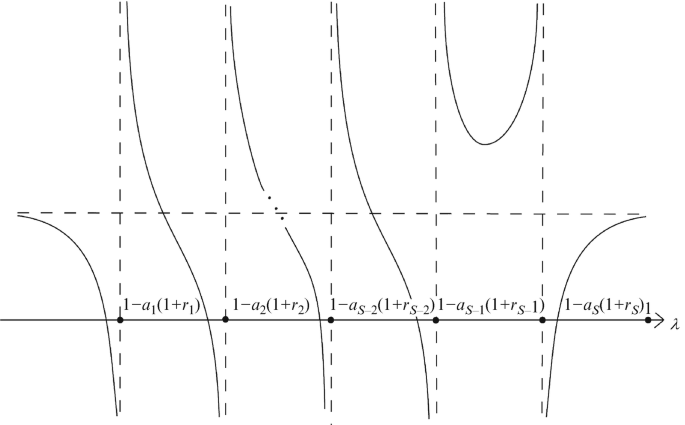

  

  The oligopoly with isoelastic price function and convex cost functions with partial adjustment towards the best response with naive expectations. The graphical determination of the eigenvalues in the case j₀ = s

  Fig. 3.3

  

  The oligopoly with isoelastic price function and convex cost functions with partial adjustment towards the best response with naive expectations. The graphical determination of the eigenvalues in the case 1 < j₀ < s

  Fig. 3.4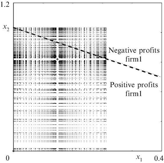

  

  Example 3.4; discrete time oligopoly with isoelastic demand and linear cost functions – the duopoly case. The cost ratio κ = c₂ ∕ c₁ = 0. 16. (a) The chaotic attractor in the (x₁, x₂) plane and the dividing line between regions of negative and positive profits for firm 1. (b) Time series of a portion of the chaotic attractor

  In the case of complex roots, no similar stability condition can be given. The possibility of complex roots will be shown later in Example 3.2.

The assumption that C_k is a convex function in its entire domain guarantees the existence of a Nash equilibrium. However if this condition is not satisfied everywhere and there is an interior equilibrium, then we have to assume that C′_k > 0 and C_k′ ≥ 0 in its neighborhood in order to assure local asymptotic stability of that equilibrium. As an illustration consider a duopoly with linear cost functions and isoelastic price function.

Example 3.2.

In this example we consider the duopoly case (N = 2). By using the notation of Example 3.1 we assume that the cost function of firm k is C_k(x_k) = d_k + c_kx_k (k = 1, 2), the price function is f(Q) = A ∕ Q with some positive constant A and the capacity limits are sufficiently large. The equilibrium is positive, since condition (3.7), that is c_k ≤ c₁ + c₂, is satisfied for both firms. Furthermore at the equilibrium

$$\bar{Q} = \frac{A} {{c}_{1} + {c}_{2}}\qquad \mbox{ and}\qquad \bar{{Q}}_{k} = \frac{A{c}_{k}} {{({c}_{1} + {c}_{2})}^{2}}.$$

From Example 1.5 we know that

$${R}_{k}({Q}_{k}) = \sqrt{\frac{A{Q}_{k } } {{c}_{k}}} - {Q}_{k},$$

and so

$${R'}_{k}(\bar{{Q}}_{k}) = \frac{{c}_{1} + {c}_{2}} {2{c}_{k}} - 1,$$

therefore

$${r}_{1} = \frac{{c}_{2} - {c}_{1}} {2{c}_{1}} \qquad \mbox{ and}\qquad {r}_{2} = \frac{{c}_{1} - {c}_{2}} {2{c}_{2}} .$$

Assume that c₁≠c₂, and that the firms select identical adjustments, that is, ${a}_{1}\,=\,{a}_{2}\,\equiv \,a$. The characteristic equation of the Jacobian of the dynamic process with partial adjustment towards the best response is given in general by (1.23), which simplifies to

$${\prod\nolimits }_{k=1}^{2}(1 - a(1 + {r}_{ k}) - \lambda )\left [1 + \frac{{r}_{1}a} {1 - a(1 + {r}_{1}) - \lambda } + \frac{{r}_{2}a} {1 - a(1 + {r}_{2}) - \lambda }\right ] = 0.$$

This equation reduces to the quadratic

$${\lambda }^{2} + \lambda (2a - 2) + (1 - 2a + {a}^{2} - {a}^{2}{r}_{ 1}{r}_{2}) = 0,$$

with roots

$${\lambda }_{1,2} = (1 - a) ia\sqrt{-{r}_{1 } {r}_{2}},$$

since

$${r}_{1}{r}_{2} = -\frac{{({c}_{1} - {c}_{2})}^{2}} {4{c}_{1}{c}_{2}} < 0.$$

By an appropriate choice of the parameters c₁ and c₂ the quantity r₁r₂ can take any negative value. Clearly if c₁≠c₂, then both roots are complex, and since

$$\vert {\lambda }_{1,2}{\vert }^{2} = 1 - 2a + {a}^{2}(1 - {r}_{ 1}{r}_{2}),$$

the roots can be both inside and outside the unit circle. The equilibrium is locally asymptotically stable if

$$a(1 - {r}_{1}{r}_{2}) < 2,$$

and unstable if this condition is violated with strict inequality. An analogous condition for the stability of the equilibrium in the duopoly case with constant adjustment speeds has been derived by Puu (2003, Chap. 7). With fixed r₁ and r₂, stability occurs if the value of a is sufficiently small. With a fixed value of a ∈ (0, 1] we have stability if the product | r₁r₂ | is sufficiently small, which holds if c₁ and c₂ are sufficiently close to each other.

Example 3.3.

Next we examine an N-firm semi-symmetric oligopoly with linear cost functions, so we assume that firms 2, 3, …, N have identical marginal costs, c_k = c₂ (k = 2, 3, …, N), identical capacity limits and common linear adjustment functions, and their initial outputs are also the same, so that x₂(0) = … = x_N(0). Given these assumptions the entire output trajectories of these firms are the same. Therefore we get a two-dimensional system with state variables x₁ and x₂ where x_k = x₂ for k ≥ 2. In this case Q₁ = (N − 1)x₂ and Q₂ = x₁ + (N − 2)x₂. Assuming that the capacity limits L_k are sufficiently large the general expressions for the equilibrium quantities given in Example 3.1 imply for the semi-symmetric case that

$$\begin{array}{rcl} \bar{{x}}_{1}& = \frac{(N-1)A} {{c}_{1}+(N-1){c}_{2}} \left (1 - \frac{(N-1){c}_{1}} {{c}_{1}+(N-1){c}_{2}} \right ) & \\ & = \frac{(N-1)A} {{c}_{1}+(N-1){c}_{2}} \left (\frac{(N-1){c}_{2}-(N-2){c}_{1}} {{c}_{1}+(N-1){c}_{2}} \right ) & \\ \bar{{x}}_{2}& = ... =\bar{ {x}}_{N} = \frac{(N-1)A} {{c}_{1}+(N-1){c}_{2}} \left (1 - \frac{(N-1){c}_{2}} {{c}_{1}+(N-117g1){c}_{2}} \right )& \\ & = \frac{(N-1)A} {{c}_{1}+(N-1){c}_{2}} \left ( \frac{{c}_{1}} {{c}_{1}+(N-1){c}_{2}} \right ). & \\ \end{array}$$

For the total industry output in equilibrium we obtain

$$\bar{Q} =\bar{ {x}}_{1} + (N - 1)\bar{{x}}_{2} = \frac{(N - 1)A} {{c}_{1} + (N - 1){c}_{2}}.$$

The derivatives of the best replies are obtained from (3.5) as

$${r}_{1} = {R'}_{1}(\bar{{Q}}_{1}) = \frac{A - 2{c}_{1}\bar{Q}} {2{c}_{1}\bar{Q}} = \frac{(N - 1){c}_{2} + (3 - 2N){c}_{1}} {2(N - 1){c}_{1}} ,$$

and

$${r}_{2} = {R'}_{2}(\bar{{Q}}_{2}) = \frac{A - 2{c}_{2}\bar{Q}} {2{c}_{2}\bar{Q}} = \frac{{c}_{1} - (N - 1){c}_{2}} {2(N - 1){c}_{2}} .$$

Conditions (3.7) for k = 1 and k = 2 are of the form

$${c}_{1} \leq \frac{{c}_{1} + (N - 1){c}_{2}} {N - 1} ,\quad {c}_{2} \leq \frac{{c}_{1} + (N - 1){c}_{2}} {N - 1} ,$$

where the second inequality always holds and the first one can be written as

$$\kappa:= \frac{{c}_{2}} {{c}_{1}} \geq\frac{N - 2} {N - 1},$$

where κ denotes the cost ratio between the firms. In addition,

$${r}_{1} = \frac{(N - 1)\kappa+ (3 - 2N)} {2(N - 1)} \quad { and}\quad {r}_{2} = \frac{1 - (N - 1)\kappa } {2(N - 1)\kappa } .$$

The dynamic process can be written as

$$\begin{array}{rcl}{ x}_{1}(t + 1)& = (1 - {a}_{1}){x}_{1}(t) + {a}_{1}{R}_{1}((N - 1){x}_{2}(t)), & \\ {x}_{2}(t + 1)& = (1 - {a}_{2}){x}_{2}(t) + {a}_{2}{R}_{2}({x}_{1}(t) + (N - 2){x}_{2}(t)),& \\ \end{array}$$

so the Jacobian has the special form

$$\left (\begin{array}{*{10}c} 1 - {a}_{1} & {a}_{1}{r}_{1}(N - 1) \\ {a}_{2}{r}_{2} & 1 - {a}_{2} + {a}_{2}{r}_{2}(N - 2) \end{array} \right )$$

where r₁ = R′₁ and r₂ = R′₂ at the equilibrium. The characteristic equation of this matrix can be written as

$$(1 - {a}_{1} - \lambda )(1 - {a}_{2} + {a}_{2}{r}_{2}(N - 2) - \lambda ) - {a}_{1}{a}_{2}{r}_{1}{r}_{2}(N - 1) = 0,$$

which can be simplified to

$$\begin{array}{rcl}{ \lambda }^{2}& +\lambda (-2 + {a}_{ 1} + {a}_{2} + (2 - N){a}_{2}{r}_{2}) + (1 - {a}_{1} - {a}_{2} + (N - 2){a}_{2}{r}_{2}& \\ & +{a}_{1}{a}_{2}(1 + (2 - N){r}_{2} + (1 - N){r}_{1}{r}_{2})) = 0. & \\ \end{array}$$

Using results from Appendix F we know that the roots are inside the unit circle if and only if

$$-{a}_{1} + {a}_{2}((N - 2){r}_{2} - 1) + {a}_{1}{a}_{2}(1 + (2 - N){r}_{2} + (1 - N){r}_{1}{r}_{2}) < 0,$$

(3.8)

$$1 + (2 - N){r}_{2} + (1 - N){r}_{1}{r}_{2} > 0,$$

(3.9)

$$4 - 2{a}_{1} + {a}_{2}(-2 + (2N - 4){r}_{2}) + {a}_{1}{a}_{2}(1 + (2 - N){r}_{2} + (1 - N){r}_{1}{r}_{2}) > 0.$$

(3.10)

The form of the stability region for (a₁, a₂) depends on the number of firms and the actual values of the derivatives r₁ and r₂. Inserting the expressions for the derivatives r₁ and r₂ given above, the stability conditions can be written in terms of the cost ratio κ = c₂ ∕ c₁, the number of firms N, and the adjustment coefficients a₁ and a₂ as

$$-4{a}_{1}\kappa (N - 1) + {a}_{1}{a}_{2}{(1 + \kappa (N - 1))}^{2} + 2{a}_{ 2}(-2 + N(1 + \kappa- \kappa N)) < 0,$$

(3.11)

$${ \left (1 + \kappa (N - 1)\right )}^{2} > 0,$$

(3.12)

$$-8(-2+{a}_{1})\kappa (N -1)+{a}_{1}{a}_{2}{(1+\kappa (N -1))}^{2} +4{a}_{ 2}(-2+N(1+\kappa -\kappa N)) > 0.$$

(3.13)

It is clear that the second inequality is always fulfilled. The properties of the stability region for (a₁, a₂) depend on the number of firms and the ratio of the firms’ unit costs.

Instead of giving a complete analysis in general we reconsider the duopoly case of Example 3.2, where a₁ = a₂ = a. In this special case the conditions (3.8)–(3.10) further simplify to

$$-2a + {a}^{2}(1 - {r}_{ 1}{r}_{2}) < 0,$$

$$1 - {r}_{1}{r}_{2} > 0,$$

and

$$4 - 4a + {a}^{2}(1 - {r}_{ 1}{r}_{2}) > 0.$$

The second and third inequalities are always satisfied, since in Example 3.2 we have shown that r₁r₂ < 0. The first relation holds if and only if

$$a(1 - {r}_{1}{r}_{2}) < 2.$$

This condition is the same as the one that was obtained earlier in Example 3.2.

The case of linear cost functions is examined in detail in the book of Okuguchi and Szidarovszky (1999) and Puu (2003).

3.1.2 Global Dynamics of Discrete Time Models

As we have seen in the discussion in Chap. 1 on concave oligopolies, the conditions for global asymptotic stability are very restrictive. In most cases of isoelastic price functions this is true as well.

Under condition (D) of Sect. 3.1, for at most one firm r_k > 0, and for all other firms, − 1 < r_k ≤ 0. If all r_k values are non-positive, then the global stability conditions are still given by (1.31). However if one r_k is positive, this condition can no longer be used, it has to be modified accordingly.

We also notice that the global stability condition given in Theorem B.3 cannot be applied either. At Q_k = 0, firm k has no best response, which is clear from its definition given in Example 1.5 and in the first part of Sect. 3.1. Therefore the set where the dynamical system

$${x}_{k}(t + 1) = {x}_{k}(t) + {\alpha }_{k}({R}_{k}({Q}_{k}(t)) - {x}_{k}(t)),\quad (k = 1,2,\ldots ,N),$$

is defined is not closed, so the contraction mapping theorem (upon which the proof of Theorem B.3 relies) cannot be used. If we consider the continuous extension by defining R_k(0) = 0, then in addition to the Nash equilibrium the zero output vector also becomes a steady state of the above dynamical system, so the presence of multiple steady states excludes the possibility of global asymptotic stability.

In this subsection we start to investigate the kinds of dynamic behavior that we can observe when the restrictive conditions for global stability are not satisfied. A characterization of the global dynamics is not trivial, since we are dealing with an N-dimensional piecewise differentiable dynamical system. Therefore, our study is based on a combination of analytical, geometrical and numerical arguments. As has been demonstrated in previous chapters, qualitative changes of the dynamics are often caused by contacts between singularities known as critical sets (see Appendix C), lines of non-differentiability, and basin boundaries. In general such contacts can only be revealed numerically, since the equations of the curves which are involved in such contacts cannot be analytically expressed in terms of elementary functions. Hence, an analysis of global bifurcations is, in general, carried out by using both theoretical and numerical methods. The occurrence of such bifurcations is shown by computer-assisted proofs, and is based on the knowledge of the properties of the singularities involved and their graphical representation (see Mira et al. (1996) for many examples and see also Brock and Hommes (1997)). This “modus operandi” is quite common in the study of the global properties of nonlinear two-dimensional discrete dynamical systems. However an extension of such methods to higher-dimensional dynamical systems is obviously limited. A practical problem which arises is that the visualization of objects in a phase space of dimension greater than two and the detection of contacts between surfaces may become very difficult. Consequently, in the examples that follow we will (again) restrict ourselves to the case of duopoly or the semi-symmetric case of an oligopoly. It should be mentioned that in the case of isoelastic demand, the non-negativity of prices is always guaranteed. So, in contrast to the oligopolies with for example linear or quadratic price functions as considered before, we do not need to ensure this property by selecting the values of the model parameters carefully. On the other hand, we still need to look at the profits along the sequence of quantity decisions in order to see if the long-run dynamics are viable from an economic point of view. Although the problem of negative profits is regularly neglected in the literature on complex dynamics in oligopolies, it is a crucial element of the analysis of an adjustment type model. The dynamical system just represents the firms’ individual production decisions, but does not directly tell us if the firms are profitable as a result of the collective outcome.

Example 3.4.

We consider again the reaction functions in the model with isoelastic demand and linear cost functions derived at the beginning of this chapter, which in the current example becomes

$${ R}_{k}({Q}_{k}) = \left \{\begin{array}{ll} 0 & { if }{z}_{k}^{{_\ast}}\leq 0{ , i.e., }{Q}_{k} \geq\frac{A} {{c}_{k}}, \\ {L}_{k} &{ if }{z}_{k}^{{_\ast}}\geq{L}_{k}{ , i.e., }{Q}_{k}^{2} + \left (2{L}_{k} - \frac{A} {{c}_{k}}\right ){Q}_{k} + {L}_{k}^{2} \leq 0, \\ {z}_{k}^{{_\ast}} = \sqrt{\frac{A{Q}_{k } } {{c}_{k}}} - {Q}_{k}&{ otherwise}, \end{array} \right .$$

(3.14)

where k = 1, …, N. Notice that the constraint z_k^∗ = L_k is ineffective if L_k ≥ A ∕ (4c_k), otherwise we have R_k = L_k for

$$\begin{array}{rcl}{ Q}_{k} \in {[}\left ( \frac{A} {2{c}_{k}} - {L}_{k}\right )& & - \frac{1} {2{c}_{k}}\sqrt{A\left (A - 4{c}_{k } {L}_{k } \right )},\left ( \frac{A} {2{c}_{k}} - {L}_{k}\right ) \\ & & + \frac{1} {2{c}_{k}}\sqrt{A\left (A - 4{c}_{k } {L}_{k } \right )}{]} \\ \end{array}$$

(see Fig. 1.9). In the duopoly case, N = 2, already considered in Example 3.2, partial adjustment towards the best response is governed by the discrete time dynamical system

$$\begin{array}{rcl}{ x}_{1}(t + 1)& = (1 - {a}_{1}){x}_{1}(t) + {a}_{1}{R}_{1}({x}_{2}),&<EquationNumber>3.15</EquationNumber> \\ {x}_{2}(t + 1)& = (1 - {a}_{2}){x}_{2}(t) + {a}_{2}{R}_{2}({x}_{1}),& \\ \end{array}$$

(3.15)

and the unique Nash equilibrium is given by

$$\bar{x} = (\bar{{x}}_{1};\bar{{x}}_{2}) = \left ( \frac{A{c}_{2}} {{({c}_{1} + {c}_{2})}^{2}}; \frac{A{c}_{1}} {{({c}_{1} + {c}_{2})}^{2}}\right ).$$

(3.16)

The local stability properties of $\bar{x}$ in the duopoly case have already been derived in Example 3.2. For identical adjustment coefficients, a₁ = a₂ = a, the equilibrium is locally asymptotically stable if a(1 − r₁r₂) < 2, where r_k = R_k′(Q_k) = (c₁ + c₂ − 2c_k) ∕ (2c_k). Inserting these expressions for the derivatives of the best replies allows us to express the stability condition in terms of the cost ratio κ = c₂ ∕ c₁ (cf. also Example 3.3 for the semi-symmetric case). Hence, in this case local asymptotic stability of the equilibrium given in (3.16) is ensured if

$$\frac{a{(1 + \kappa )}^{2}} {4\kappa } < 2.$$

Consequently, for any given a ∈ (0, 1], as long as

$$\kappa\in \left (\frac{4 - a - 2\sqrt{4 - 2a}} {a} , \frac{4 - a + 2\sqrt{4 - 2a}} {a} \right )$$

holds, the equilibrium is stable. Note that since κ = 1 is always inside this interval for all adjustment coefficients a ∈ (0, 1], the equilibrium is always stable if firms have identical marginal costs. It is also worth pointing out that the cost difference between the firms has to be quite strong in order to render the equilibrium unstable. To demonstrate this, we look at a particular case of the best reply dynamics, namely a₁ = a₂ = 1. Here the Nash equilibrium (3.16) is stable if and only if the cost ratio $\kappa= {c}_{2}/{c}_{1} \in(3 - 2\sqrt{2},3 + 2\sqrt{2}) \simeq \left (0.17,5.83\right )$ (see also Puu (1991, 2003)). If, for example, c₁ = 1, this result shows that the unit cost of firm 2 has to be either at least almost 6 times higher than firm 1’s unit cost or less than about 1 ∕ 6 of it in order that instability occurs. If the cost ratio c₂ ∕ c₁ exits this interval, then the Nash equilibrium loses stability via a period doubling bifurcation. For values of the cost ratio outside the interval $(3 - 2\sqrt{2},3 + 2\sqrt{2})$ the asymptotic dynamics may converge to periodic cycles or even exhibit chaotic motion around the Nash equilibrium. A numerically computed chaotic trajectory is shown in Fig. 3.4, obtained for A = 1, a₁ = a₂ = 1, c₁ = 1, c₂ = 0. 16. It can be noticed that the chaotic area is quite large, hence we expect no correlations between x₁(t) and x₂(t), in the sense that high values of x₁(t) are associated either with high or with low values of x₂(t) in the same time period; see Fig. 3.4b, where a portion of the chaotic trajectory of Fig. 3.4a is represented for the time periods t ∈ 300, 370. Note that the profits for the firms are non-negative only if x₁ + x₂ ≤ A ∕ c_k, k = 1, 2. In Fig. 3.4a we depict the line of zero profits for firm 1, which is represented by the equation x₁ + x₂ = A ∕ c₁ = 1. Notice that the zero profit line of firm 2, x₁ + x₂ = 6. 25, is outside the area shown in the figure. This indicates that the profits for the low-cost firm 2 are always positive, whereas firm 1 makes a loss in some periods along any trajectory which describes the long-run dynamics. The latter point becomes even more obvious if we consider other kinds of long-run dynamics for the duopoly with best reply dynamics. For example, let c₂ = 0. 161, with all other parameter values as before. The cost ratio is now outside the stability region, and the disequilibrium dynamics in this case are described by a 4-cyclic chaotic attractor¹ (see Fig. 3.5²). Of course, even if in this case chaotic dynamics are observed, the time series are much more regular, since they are characterized by a quasi-cyclic behavior (Fig. 3.5b). Furthermore, the zero profit line for firm 1 depicted in Fig. 3.5a indicates that the high-cost firm 1 would make a loss after every fourth period with certainty, and potentially also makes a loss after every third period. Consequently, given the regularity of the trajectories in this situation and the possibility of losses following a regular pattern, it seems that the assumption of naive expectations would be more plausible in the former case, where the chaotic attractor extends over a larger portion of the phase space.

Fig. 3.5

Example 3.4; discrete time oligopoly with isoelastic demand and linear cost functions – the duopoly case. The cost ratio κ = c₂ ∕ c₁ = 0. 161. (a) A 4-cyclic chaotic attractor in the (x₁, x₂) plane and dividing line between regions of positive and negative profits for firm 1. (b) Time series of a portion of the chaotic attractor. Note how they are more regular than those in Fig. 3.4b

Let us now turn to the semi-symmetric case obtained by assuming c₂ = . . .= c_N, a₂ = . . .= a_N, L₂ = . . .= L_N and x₂(0) = . . .= x_N(0). This particular situation, which has been already studied in Example 3.3, allows us to get some insight into the effects of increasing the number of competitors. As we have seen already in the previous chapters, if the firms partially adjust their production quantities towards the best replies, then the decisions made by firm 1 and the identical firms 2, …, N are captured by the two-dimensional dynamical system

$$ T : \left \{\begin{array}{l} {x}_{1}(t + 1) = (1 - {a}_{1}){x}_{1}(t) + {a}_{1}{R}_{1}((N - 1){x}_{2}), \\ {x}_{2}(t + 1) = (1 - {a}_{2}){x}_{2}(t) + {a}_{2}{R}_{2}({x}_{1} + (N - 2){x}_{2}). \end{array} \right . $$

Assuming an interior equilibrium, it is given by

$$ \begin{array}{rcl} \bar{{x}}_{1}& = \frac{(N-1)A} {{c}_{1}+(N-1){c}_{2}} \left (\frac{(N-1){c}_{2}-(N-2){c}_{1}} {{c}_{1}+(N-1){c}_{2}} \right ), & \\ \bar{{x}}_{2}& = ... =\bar{ {x}}_{N} = \frac{(N-1)A} {{c}_{1}+(N-1){c}_{2}} \left ( \frac{{c}_{1}} {{c}_{1}+(N-1){c}_{2}} \right )& \\ \end{array} $$

and it is locally asymptotically stable if

$$ \begin{array}{rcl} & \qquad - 4{a}_{1}\kappa (N - 1) + {a}_{1}{a}_{2}{(1 + \kappa (N - 1))}^{2} + 2{a}_{2}(-2 + N(1 + \kappa- \kappa N)) < 0 & \\ & -8(-2 + {a}_{1})\kappa (N - 1) + {a}_{1}{a}_{2}{(1 + \kappa (N - 1))}^{2}+4{a}_{2}(-2+N(1 + \kappa -\kappa N)) > 0,&<EquationNumber>3.17</EquationNumber>\\ \end{array} $$

(3.17)

where κ = c₂ ∕ c₁ denotes the cost ratio between firms (see Example 3.3; recall that the other stability condition derived there is always fulfilled). For given adjustment coefficients and unit costs, these conditions tell us for which number of firms the equilibrium becomes unstable. Consider for example A = 16, a₁ = 0. 4, a₂ = 0. 3, c₁ = 5, c₂ = 6, L₁ = L₂ = 2. Then it is easy to see that the first condition holds always for N > 2, so we do not consider it in the following analysis. The second inequality becomes − 88N² + 1246(N − 1) > 0, and it holds as long as the number of firms N ≤ 13. So in these cases the equilibrium is stable. For N = 14 this inequality is violated, showing that the equilibrium becomes unstable. Figure 3.6 shows a bifurcation diagram for N in the range 2, 30. As expected, the Nash equilibrium $\bar{x}$ is stable as long as the number of competitors is less than 13, and then it loses stability through a period doubling bifurcation . For even higher values of N other bifurcations occur leading to more complicated kinds of asymptotic behavior. Since more detailed results can be easily derived on the basis of a standard local stability analysis, we now turn to the more interesting investigation of the global properties of our model.

Fig. 3.6

Example 3.4; discrete time oligopoly with isoelastic demand and linear cost functions – the semi-symmetric case. Bifurcation diagrams of outputs x₁, x₂ with respect to the number of firms

In order to explain what kind of bifurcations and global dynamic properties are involved in the qualitative changes of the dynamics observed in Fig. 3.6, we study the properties of the piecewise smooth map T. We first divide the strategy space $\mathbb{D} =\left [0,{L}_{1}\right ] \times \left [0,{L}_{2}\right ]$ into regions ${\mathbb{D}}^{(k)}$ where the map T has different expressions. As observed in Chap. 1, the curves that divide these regions are curves of non-differentiability, and these curves may play the role of folding curves (or critical curves, following the terminology used in Mira et al. (1996)). In order to write the expression of the map T in the different regions ${\mathbb{D}}^{(k)}$, notice that for the set of parameters considered, in the expression of the reaction curve (3.14) of firm 1 we have

$${z}_{1}^{{_\ast}} < 0{ for }{x}_{ 2} > \frac{16} {5\left (N - 1\right )},$$

whereas the constraint z₁^∗ > L₁ is ineffective since L₁ > A ∕ (4c₁). Likewise, for the reaction function R₂ of firms 2, …, N, we have

$${z}_{2}^{{_\ast}} < 0{ for }{x}_{ 1} + \left (N - 2\right ){x}_{2} > 8/3$$

and the constraint z₂^∗ > L₂ is ineffective since L₂ > A ∕ (4c₂). The lines ${x}_{2} = \frac{16} {5\left (N-1\right )}$ and ${x}_{2} = \frac{8-3{x}_{1}} {3\left (N-2\right )}$ divide the strategy space $\mathbb{D}$ into 4 regions. In region ${\mathbb{D}}^{(1)}$, where ${x}_{2} < \frac{16} {5\left (N-1\right )}$ and ${x}_{2} < \frac{8-3{x}_{1}} {3\left (N-2\right )}$, we have

$$T{\vert }_{{\mathbb{D}}^{(1)}} : \left \{\begin{array}{l} {x}_{1}(t + 1) = (1 - {a}_{1}){x}_{1}(t) + {a}_{1}\left [\sqrt{\frac{16(N-1){x}_{2 } (t)} {5}} - (N - 1){x}_{2}(t)\right ], \\ beginequation{_\ast}8pt]{x}_{2}(t + 1) = (1 - {a}_{2}){x}_{2}(t) + {a}_{2}{[}\sqrt{\frac{16({x}_{1 } (t)+(N-2){x}_{2 } (t))} {6}} - {x}_{1}(t) \\ \qquad \qquad \quad - (N - 2){x}_{2}(t){]}. \end{array} \right .$$

In region ${\mathbb{D}}^{(2)}$, where x₂ < \frac{16} __ {5N − 1} and x₂ > \frac{8 − 3x₁} {3N − 2} , the map is

$$T{\vert }_{{\mathbb{D}}^{(2)}} : \left \{\begin{array}{l} {x}_{1}(t + 1) = (1 - {a}_{1}){x}_{1}(t) + {a}_{1}\left [\sqrt{\frac{16(N-1){x}_{2 } (t)} {5}} - (N - 1){x}_{2}(t)\right ], \\ {x}_{2}(t + 1) = (1 - {a}_{2}){x}_{2}(t). \end{array} \right .$$

In region ${\mathbb{D}}^{(3)}$, where x₂ > \frac{16} __ {5N − 1} and x₂ > \frac{8 − 3x₁} {3N − 2} , the map is

$$T{\vert }_{{\mathbb{D}}^{(3)}} : \left \{\begin{array}{c} {x}_{1}(t + 1) = (1 - {a}_{1}){x}_{1}(t), \\ {x}_{2}(t + 1) = (1 - {a}_{2}){x}_{2}(t). \end{array} \right .$$

In region ${\mathbb{D}}^{(4)}$, where x₂ > \frac{16} __ {5N − 1} and x₂ < \frac{8 − 3x₁} {3N − 2} , we have

$$T{\vert }_{{\mathbb{D}}^{(4)}} : \left \{\begin{array}{l} {x}_{1}(t + 1) = (1 - {a}_{1}){x}_{1}(t), \\ {x}_{2}(t + 1) = (1 - {a}_{2}){x}_{2}(t) + {a}_{2}{[}\sqrt{\frac{16({x}_{1 } (t)+(N-2){x}_{2 } (t))} {6}} - {x}_{1}(t) \\ \qquad \qquad \quad - (N - 2){x}_{2}(t){]}. \end{array} \right .$$

The positive equilibrium

$$\bar{x} = \left (\frac{16\left (N - 1\right )\left (N + 4\right )} {{\left (6N - 1\right )}^{2}} , \frac{80\left (N - 1\right )} {{\left (6N - 1\right )}^{2}} \right )$$

is in region ${\mathbb{D}}^{(1)}$, whereas no equilibria exist in regions ${\mathbb{D}}^{(k)}$, k = 2, 3, 4. In order to study the local stability of the positive fixed point \bar{x}, we consider the Jacobian matrix

$${{{ J}}}^{(1)} = \left (\begin{array}{cc} 1 - {a}_{1} & {a}_{1}\left [ \frac{2\left (N-1\right )} {\sqrt{5(N-1){x}_{2}}} - (N - 1)\right ] \\ {a}_{2}\left [ \frac{\sqrt{2}} {\sqrt{3\left [{x}_{1 } +(N-2){x}_{2 } \right ]}} - 1\right ]&1 - {a}_{2} + \left (N - 2\right ){a}_{2}\left [ \frac{\sqrt{2}} {\sqrt{3\left [{x}_{1 } +(N-2){x}_{2 } \right ]}} - 1\right ] \end{array} \right )$$

(3.18)

computed at \bar{x}. Using the characteristic equation, the stability condition − 88N² + 1246(N − 1) > 0 given before follows after some calculation. As noticed above, the equilibrium \bar{x} undergoes a flip (or period doubling) bifurcation for increasing N. After the first flip bifurcation, occurring at N ≃ 13, further period doublings occur and a route towards chaotic behavior is observed for increasing values of N. However, it is obvious from the stability conditions in (3.17) that the values of the two speeds of adjustment also play an important role. Stability of the positive equilibrium is always ensured for appropriately selected low values of the adjustment speed a₂. This can also be confirmed by numerical simulations. In Fig. 3.7 we show a bifurcation diagram obtained with N = 23, where all the other parameters are chosen as in Fig. 3.6 and with the bifurcation parameter a₂ spanning the whole range (0, 1]. For low values of a₂ the equilibrium is stable. For increasing values of a₂ several sudden transitions between chaotic and periodic behavior characterize the asymptotic dynamics. Many of these bifurcations are different from the common bifurcations observed for smooth dynamical systems as the reader might notice. The reason is that the bifurcations observed here are strongly influenced by the presence of the lines of non-differentiability. As already stressed in Chap. 1, these can be often classified as border collision bifurcations, occurring when an equilibrium point (or a periodic point) of a piecewise differentiable dynamical system crosses a curve of non-differentiability. Such a contact may produce many kinds of effects (transition to another cycle of any period or a sudden transition to chaos) depending on the eigenvalues of the two Jacobian matrices on the two adjacent sides of the curve of non-differentiability involved in the contact (see for example, Banerjee et al. (2000b)).

Fig. 3.7

Example 3.4; discrete time oligopoly with isoelastic demand and linear cost functions – the semi-symmetric case. Bifurcation diagrams of outputs x₁, x₂ with respect to a₂ with the number of firms held fixed at N = 23. The parameters are otherwise as in Fig. 3.6

Moreover, as we have shown in Chap. 1 (see also Appendix C) the lines of non-differentiability may represent “folding lines,” and consequently they have a role similar to that of the critical curves, where the latter are defined as sets of points where the Jacobian determinant vanishes. In other words, candidates for the “folding curves” F⁽ⁱ⁾ in the particular example we are considering are:

• The curves of non-differentiability, that is the lines x₂ = \frac{16}__ {5N − 1} and x₂ = \frac{8 − 3x₁} {3N − 2} ;

• The curves of vanishing Jacobian, where the Jacobian matrices in the regions ${\mathbb{D}}^{(k)}$, k = 1, …, 4, are respectively J⁽¹⁾, given in (3.18),

  $${ J}^{(2)} = \left (\begin{array}{cc} 1 - {a}_{1} & {a}_{1}\left ( \frac{2\left (N-1\right )} {\sqrt{5(N-1){x}_{2}}} - (N - 1)\right ) \\ 0 & 1 - {a}_{2}\end{array} \right ),$$
  $${ J}^{(3)} = \left (\begin{array}{cc} 1 - {a}_{1} & 0 \\ 0 &1 - {a}_{2}\end{array} \right ),$$

  and

  $${ J}^{(4)} = \left (\begin{array}{cc} 1 - {a}_{1} & 0 \\ {a}_{2}\left ( \frac{\sqrt{2}} {\sqrt{3\left [{x}_{1 } +(N-2){x}_{2 } \right ]}}-1\right )&1-{a}_{2} + \left (N-2\right ){a}_{2}\left ( \frac{\sqrt{2}} {\sqrt{3\left [{x}_{1 } +(N-2){x}_{2 } \right ]}}-1\right ) \end{array} \right ).$$

Notice that only in regions ${\mathbb{D}}^{(1)}$ and ${\mathbb{D}}^{(4)}$ may we have points at which the Jacobian determinant vanishes.

Fig. 3.8

Example 3.4; discrete time oligopoly with isoelastic demand and linear cost functions. Global dynamics in the semi-symmetric case. (a) At a₂ ≃ 0. 2466 a border collision bifurcation occurs when one of the two periodic points intersects the “folding line” F and a 4-piece chaotic attractor is born. (b) As a₂ increases to a₂ = 0. 26 the chaotic attractor intersects a “folding line”

After the foregoing preparations, we are now in a position to describe some border collision bifurcations as well as some methods to bound chaotic attractors that involve the lines of non-differentiability for a specific numerical example. Let us start from the set of parameters used to obtain the bifurcation diagram Fig. 3.7, that is N = 23, A = 16, a₁ = 0. 4, c₁ = 5, c₂ = 6, L₁ = L₂ = 2. From the second stability condition in (3.17) we can deduce that at a₂ = \frac{21120}_ {127781} ≃ 0. 165 the Nash equilibrium \bar{x} loses stability through a flip bifurcation, at which it becomes a saddle point, and a stable cycle of period 2 is created around it. Just after this bifurcation, the two periodic points are close to the saddle point \bar{x}, hence they belong to region ${\mathbb{D}}^{(1)}$. As the parameter a₂ is further increased, the two periodic points move away from the fixed point, and one of them intersects the boundary of region ${\mathbb{D}}^{(1)}$, denoted as “folding line” F in Fig. 3.8. This first border crossing may produce many kinds of effects. However, in this case there are no evident effects: if one of the periodic points moves into region ${\mathbb{D}}^{(2)}$ (while the other remains in region ${\mathbb{D}}^{(1)}$), the 2-cycle remains attracting. This is an example of a border collision without any change in the qualitative dynamics. At a₂ ≃ 0. 2462 the 2-cycle undergoes a flip bifurcation and a stable cycle of period 4 appears. As before, just after the bifurcation the four periodic points are close to the 2-cycle saddle, and far from the lines of non-differentiability. However, as the parameter a₂ is further increased, one of the periodic points moves towards the folding line F, and at a₂ ≃ 0. 2466, a periodic point intersects the boundary of region ${\mathbb{D}}^{(1)}$, that is the “folding line” F (see Fig. 3.8a). This marks the occurrence of a true border collision bifurcation, with the effect of a transition to a 4-piece chaotic attractor (see Fig. 3.8b with a₂ = 0. 26).

As can be seen, the chaotic attractor crosses the folding line F. Hence, it is bounded by the images of this line, denoted as T⁽ⁱ⁾(F), i = 1…, 8, in Fig. 3.8b. This suggests that when a chaotic attractor intersects a folding line F, the boundary of the chaotic area includes points belonging to images of increasing rank of F. This is a well-known property of the critical lines of smooth noninvertible maps (see Appendix C), which is here extended to the lines of non-differentiability of a piecewise differentiable map (see Mira et al. (1996)). As a₂ is further increased, the 4-cyclic chaotic attractor becomes wider (see Fig. 3.9a) until the merging of the pieces occurs. This merging leads to a 2-cyclic chaotic attractor (this occurs at a₂ ≃ 0. 2765) and then a unique large chaotic attractor emerges (see Fig. 3.9b), obtained for a₂ ≃ 0. 2965). Also in this case, the boundary of the chaotic area is given by the images of a suitable portion of the folding line F. Finally, we once again point out that in the two cases shown in Fig. 3.9, the upper portion of the chaotic attractors is included in the region with negative profits, that is above the lines representing the equation x₁ + (N − 1)x₂ = A ∕ c_k, k = 1, 2. This means that along the chaotic trajectories that describe the long run time evolution of the production decisions of the firms, some periods with negative profits are involved.

Fig. 3.9

Example 3.4; discrete time oligopoly with isoelastic demand and linear cost functions. Global dynamics in the semi-symmetric case. Parameters are the same as in Fig. 3.8. (a) As a₂ increases further to a₂ ≃ 0. 2765 the pieces of the chaotic attractor merge into a 2-cyclic chaotic attractor. (b) At a₂ ≃ 0. 2965 a unique large chaotic attractor emerges

3.1.3 Continuous Time Models and Local Stability

In this section model (1.31), describing the continuous time dynamics of partial adjustment towards the best response with naive expectations, is examined in the isoelastic case. The Jacobian of the system again has the form (1.46), and its characteristic equation has the special form of (1.47). We assume again that a_k = α′_k(0) > 0 for all k. Here either all r_k values are in the interval ( − 1, 0], or exactly one r_k value is positive. If none of the r_k values is positive, then the local asymptotic behavior of the equilibrium is the same as in the concave case. By adding up the terms with identical denominators in the bracketed factor of (1.47) we obtain (1.48), where at most one θ_j > 0. If all θ_j ≤ 0, then the problem is the same as in the concave case, so the equilibrium is always locally asymptotically stable. Therefore we may assume that ${\theta }_{{j}_{0}}\,>\,0$ for some j₀. If θ_j≠0 and m_j = 1, then − a_j(1 + r_j) is not an eigenvalue of the Jacobian. Otherwise it is, and the other eigenvalues are the roots of the equation

$$1 -{\sum\nolimits }_{j=1}^{s} \frac{{\theta }_{j}} {{a}_{j}(1 + {r}_{j}) + \lambda } = 0,\qquad \qquad$$

where we assume again that θ_j≠0 for all j, a_k > 0 for all firms, and

$${a}_{1}(1 + {r}_{1}) > {a}_{2}(1 + {r}_{2}) > \ldots> {a}_{s}(1 + {r}_{s}).$$

If g(λ) denotes again the left hand side of the above equation, then

$${ \lim }_{\lambda \rightarrow \pm \infty }g(\lambda ) = 1,$$

$${ \lim }_{\lambda \rightarrow -{a}_{j}(1+{r}_{j})\pm 0}g(\lambda ) = \begin{cases} \mp \infty & {{\rm{if}} j = {j}_{0}},\\ \pm \infty & {{\rm{if}} j\neq {j}_{0}.}\\ \end{cases}$$

However similarly to the discrete time case, g′(λ) has no definite sign. The graph of g(λ) is the same as shown earlier in Figs. 3.1–3.3 with the only difference being that the poles are all negative and given by − a₁(1 + r₁), …, − a_s(1 + r_s). Therefore we have again three cases.

• If j₀ = 1, then there are s − 2 real roots between each pair of poles − a_j(1 + r_j) and − a_{j + 1}(1 + r_{j + 1}) for j = 2, …, s − 1. If the other two roots are real and are between − a₁(1 + r₁) and − a_s(1 + r_s), then the equilibrium is locally asymptotically stable.

• If j₀ = s, then all roots are real and are negative if g(0) > 0. This condition can be rewritten as

  $${\sum\nolimits }_{k=1}^{N} \frac{{r}_{k}} {1 + {r}_{k}} < 1.$$

• If 1 < j₀ < s, then there are s − 2 real roots, one before − a₁(1 + r₁), and one in between each pair of poles − a_j(1 + r_j) and − a_{j + 1}(1 + r_{j + 1}) for j = 1, …, j₀ − 2, j₀ + 1, …, s − 1. If we assume that the remaining two roots are real and between − a₁(1 + r₁) and − a_s(1 + r_s), then all roots are negative.

The possibility of complex roots will be shown later in Example 3.6. If there are complex roots, then no simple stability conditions can be given. We will next return to the case of Example 3.3, but under the assumption of continuous time dynamics.

Example 3.5.

Consider again the N-person semi-symmetric oligopoly of Example 3.3, now under the assumption of continuous time adjustment of the outputs of the firms of the oligopoly. Assume again that c₂ = . . .= c_N. Then Q₁ = (N − 1)x₂ and Q₂ = x₁ + (N − 2)x₂ by assuming that firms 2, …, N select identical linear adjustment function and initial outputs. From Example 3.3 we know that at the interior equilibrium

$$\begin{array}{rcl} \bar{Q}& = \frac{(N-1)A} {{c}_{1}+(N-1){c}_{2}} , & \\ {r}_{1}& = {R'}_{1}(\bar{{Q}}_{1}) = \frac{(N-1){c}_{2}+(3-2N){c}_{1}} {2(N-1){c}_{1}} ,& \\ {r}_{2}& = {R'}_{2}(\bar{{Q}}_{2}) = \frac{{c}_{1}-(N-1){c}_{2}} {2(N-1){c}_{2}} . & \\ \end{array}$$

Condition (3.7) for k = 1 and k = 2 is

$${c}_{1} \leq \frac{{c}_{1} + (N - 1){c}_{2}} {N - 1} ,\quad {c}_{2} \leq \frac{{c}_{1} + (N - 1){c}_{2}} {N - 1} .$$

The second inequality always holds, the first can be rewritten as

$$\frac{{c}_{2}} {{c}_{1}} \geq\frac{N - 2} {N - 1}.$$

(3.19)

By introducing again the notation κ = c₂ ∕ c₁ we have

$$\begin{array}{rcl} \kappa & \geq\frac{N-2} {N-1}, & \\ {r}_{1}& = \frac{(N-1)\kappa +(3-2N)} {2(N-1)} { and }{r}_{2} = \frac{1-(N-1)\kappa } {2(N-1)\kappa } .& \\ \end{array}$$

The two-dimensional system for the adjustment of firms’ outputs has the form

$$\begin{array}{rcl} \dot{{x}}_{1}& = {a}_{1}({R}_{1}((N - 1){x}_{2}) - {x}_{1}), & \\ \dot{{x}}_{2}& = {a}_{2}({R}_{2}({x}_{1} + (N - 2){x}_{2}) - {x}_{2}),& \\ \end{array}$$

with Jacobian matrix

$$\left (\begin{array}{*{10}c} -{a}_{1} & {a}_{1}{r}_{1}(N - 1) \\ {a}_{2}{r}_{2} & {a}_{2}({r}_{2}(N - 2) - 1) \end{array} \right ).$$

The characteristic equation can be written as

$$(-{a}_{1} - \lambda )({a}_{2}({r}_{2}(N - 2) - 1) - \lambda ) - {a}_{1}{a}_{2}{r}_{1}{r}_{2}(N - 1) = 0$$

or

$${\lambda }^{2} + \lambda [{a}_{ 1} + {a}_{2}(1 + {r}_{2}(2 - N))] + {a}_{1}{a}_{2}[1 + (2 - N){r}_{2} - (N - 1){r}_{1}{r}_{2}] = 0.$$

(3.20)

Clearly,

$${r}_{2} \leq \frac{1 - (N - 1){N - 2} {N - 1}} {2(N - 1)\kappa } = \frac{3 - N} {2(N - 1)\kappa }.$$

Notice first that the linear coefficient of (3.20) is always positive since r₂ ≤ 0. With the new variable $\mathcal{K} = (N - 1)\kappa$, the multiplier of a₁a₂ in the constant term of (3.20) has the form

$$\begin{array}{rcl} 1 + (2 - N)\frac{(1 -\mathcal{K})} {2\mathcal{K}} - (N - 1)\frac{(\mathcal{K} + (3 - 2N))} {2(N - 1)} \frac{1 -\mathcal{K}} {2\mathcal{K}} & & \\ = \frac{1} {4\mathcal{K}}[4\mathcal{K} + (4 - 2N)(1 -\mathcal{K}) - (1 -\mathcal{K})(\mathcal{K} + 3 - 2N)] = \frac{{(\mathcal{K} + 1)}^{2}} {4\mathcal{K}} > 0.& & \\ \end{array}$$

Then Lemma F.2 implies that the equilibrium is always locally asymptotically stable.

Example 3.6.

Assume in the previous example that N = 2, a₁ = a₂ = a. Then (3.20) simplifies to

$${\lambda }^{2} + 2a\lambda+ {a}^{2}(1 - {r}_{ 1}{r}_{2}) = 0.$$

From Example 3.2 we know that r₁r₂ < 0 if c₁≠c₂. In this case both the linear and constant coefficients are positive (as in the general case of the previous example), and the discriminant is

$$4{a}^{2} - 4{a}^{2}(1 - {r}_{ 1}{r}_{2}) = 4{a}^{2}{r}_{ 1}{r}_{2} < 0.$$

So both roots are complex, showing that there is no guarantee that the eigenvalues are real, contrary to the case of concave oligopolies discussed in Sect. 1.5.

The book by Okuguchi and Szidarovszky (1999) contains some stability results in the case of linear cost functions. A detailed stability analysis is presented by Chiarella and Szidarovszky (2002) for the general nonlinear case. Models with continuously distributed time lags are identical to the concave case, so the derivations and the similar results are not duplicated here.

3.2 Cost Externalities and Multiple Interior Nash Equilibria

In Chap. 1 we demonstrated that under some standard assumptions on the demand function and on the cost functions of the oligopolists, the reaction functions of the firms are decreasing. However, there are several situations where the microeconomic fundamentals of an oligopoly model lead to reaction functions which are non-monotonic. For example, in the previous subsection we have shown that with isoelastic price functions the reaction functions are increasing over the range where the expected aggregate quantity of the other players is small, otherwise it is decreasing (see also Example 1.5 and Bulow et al. (1985b)). Using non-monotonic reaction functions, several authors have considered the best response dynamics and the partial adjustment towards the best response and have demonstrated that such adjustment processes may lead to non-convergence with complicated, but bounded fluctuations of the production sequences (for example, Rand (1978), Dana andMontrucchio (1986), Witteloostuijn and Lier (1990) and Puu (1991)). The focus of these contributions has been mainly towards questions of local stability of the Nash equilibria and the creation of complex attractors if convergence to an equilibrium fails. The emphasis of the analysis is, in this case, on the delineation of a trapping region in the space of production quantities, where the asymptotic dynamics of the oligopoly game are ultimately bounded.

In the present subsection we will turn our attention to externalities in the cost functions, which might also give rise to non-monotonic reaction functions (see Example 1.6, Kopel (1996), Puhakka and Wissink (1995), Bischi and Lamantia (2002) and Furth (1986, 2009)). We will consider a duopoly market and we will show that in a simple model with cost externalities we obtain several coexisting equilibria. Since an equilibrium point can be considered as a convention that arises among firms interacting repeatedly, stability arguments are often used to solve this coordination problem. See for example, Van Huyck and Battalio (1998) and Van Huyck et al. (1984, 1997). If a stability argument selects a single equilibrium, this point can be considered as the solution of the oligopoly game. However, as we will see, in the model with cost externalities multiple equilibria survive this type of refinement and several (locally) stable equilibria coexist. Each of these equilibria has its own basin of attraction and, consequently, the dynamic process becomes path dependent. The long run outcome of the players’ myopic output decisions crucially depends on the initial production quantity. Hence, in such a situation it is not sufficient to analyze the local stability properties. In order to be able to give some insight into the long run market outcome, it is important to gain some knowledge about the boundaries that separate the basins of attraction of the various coexisting equilibria, and to study the role of these boundaries in the occurrence of global bifurcations that drastically change the topological structure of the basins.

Recall from Example 1.6 that if the inverse demand function is linear, p = f(Q) = A − BQ, and the cost functions of the oligopolists are characterized by interfirm externalities, that is C_k(x_k, Q_k) = x_kM_k(Q_k) with M_k(Q_k) = A − B(1 + 2μ_k)Q_k − 2Bμ_kQ_k², then the best response of firm k is given by

$${ R}_{k}({Q}_{k}) = \left \{\begin{array}{ccc} 0 & { if} & {\mu }_{k}{Q}_{k}(1 - {Q}_{k}) \leq 0, \\ {L}_{k} & { if} &{\mu }_{k}{Q}_{k}(1 - {Q}_{k}) \geq{L}_{k}, \\ {z}_{k}^{{_\ast}}&{ otherwise},& \end{array} \right .$$

where z_k^∗ = μ_kQ_k(1 − Q_k) and L_k denotes the capacity of firm k. The parameters μ_k measure the intensity of the interfirm cost externality (see Kopel (1996)). In what follows we consider a duopoly market (N = 2), so that Q₁ = x₂ and Q₂ = x₁. We let μ_k ∈ (1, 4] and for simplicity we assume that L_k = 1. Under these assumptions the reaction functions reduce to

$${R}_{1}\left ({x}_{2}\right ) = {\mu }_{1}{x}_{2}\left (1 - {x}_{2}\right ),\quad {R}_{2}\left ({x}_{1}\right ) = {\mu }_{2}{x}_{1}\left (1 - {x}_{1}\right ).$$

(3.21)

The Nash equilibria of this duopoly are located at the intersections of the two reaction curves x₁ = R₁(x₂) and x₂ = R₂(x₁). The reaction functions are shown in Fig. 3.10, where the two panels illustrate that beside the trivial Nash equilibrium O = 0, 0, multiple interior Nash equilibria can exist depending on the level of the cost externalities. For example, for μ₁ = 3, μ₂ = 3. 5 there is just one interior Nash equilibrium E_S (part (a)), whereas for μ₁ = 3. 7, μ₂ = 3. 5 there are two additional interior Nash equilibria E₁ and E₂ (part (b)). Analytically, the interior equilibria are obtained as the real solutions of the fourth degree algebraic system

$${x}_{1} = {\mu }_{1}{x}_{2}\left (1 - {x}_{2}\right ),\quad {x}_{2} = {\mu }_{2}{x}_{1}\left (1 - {x}_{1}\right ),$$

and this system can have up to four solutions.

Fig. 3.10

Oligopolies with linear inverse demand function and cost externalities. The case of duopoly, multiple Nash equilibria become a possibility. (a) A unique interior Nash equilibrium occurs when μ₁ = 3, μ₂ = 3. 5. (b) Three interior Nash equilibria occur when μ₁ = 3. 7, μ₂ = 3. 5

In order to keep the following analysis tractable, we make the (rather reasonable) assumption that the influence of each firm’s action on the marginal costs of the competitor is identical for both firms, that is

$${\mu }_{1} = {\mu }_{2} = \mu .$$

(3.22)

In the case of μ > 1 there is always an interior Nash equilibrium E_S which belongs to the diagonal $\Delta= \left \{\left (x,x\right ),x \in\mathbb{R}\right \}$. Its coordinates are given by

$${E}_{S} = \left (1 - \frac{1} {\mu },1 - \frac{1} {\mu }\right ),$$

and it is characterized by identical production quantities of the two firms. At μ > 3 two further Nash equilibria exist. They are given by

$$\begin{array}{l} {E}_{1} = \left ({\mu+ 1 + \sqrt{\left (\mu+ 1 \right ) \left (\mu- 3 \right )}} {2\mu } , {\mu+ 1 -\sqrt{\left (\mu+ 1 \right ) \left (\mu- 3 \right )}} {2\mu } \right ), \\ {E}_{2} = \left ({\mu+ 1 -\sqrt{\left (\mu+ 1 \right ) \left (\mu- 3 \right )}} {2\mu } , {\mu+ 1 + \sqrt{\left (\mu+ 1 \right ) \left (\mu- 3 \right )}} {2\mu } \right ), \end{array}$$

(3.23)

and they are located in symmetric positions with respect to the diagonal Δ. Notice that for μ = 3, E₁, E₂ and E_S coincide. These Nash equilibria are characterized by different production quantities of the two players. It is easy to see that the market share of firm 1 (firm 2) is larger in E₁ (E₂). Obviously, in a situation where multiple Nash equilibria coexist, a coordination problem for the two firms arises. It is not clear which of the Nash equilibria the firms can agree upon as an outcome of the game. One possibility to discriminate among the equilibria is to assume that players start with quantity pairs out of equilibrium and adjust their production decision to evolving changes in their environment, for example, using their best replies or estimates of the gradient of the profit functions. Then we can use local stability, global dynamics, or for example, the extent of the basins of attraction in the case of multiple locally stable equilibria to obtain insights into the question about which of the equilibria is more likely to be a long run outcome of the game (see Kopel (2009) and Cox and Walker (1998)).

We will assume that in order to update their production decisions, the duopolists use partial adjustment towards the best response with naive expectations. Recall, however, that in Chap. 1 we have shown that in the duopoly case the best reply dynamics with adaptive expectations is identical to the dynamical system obtained by partial adjustment towards the best response with naive expectations (see (1.20) and (1.21)). Consequently, for our duopoly model with symmetric cost externalities, in either case the dynamical systems which generates the sequences of (expected) production quantities is given by

$$\begin{array}{l} {x}_{1}(t+1) = (1-{a}_{1}){x}_{1}(t)+{a}_{1}{R}_{1}({x}_{2}(t))=\left (1\,-\,{a}_{1}\right ){x}_{1}\left (t\right ) + {a}_{1}\mu {x}_{2}(t)\left (1 - {x}_{2}(t)\right ),\\ \\ {x}_{2}(t+1) = (1 - {a}_{2}){x}_{2}(t)+{a}_{2}{R}_{2}({x}_{1}(t)) = (1-{a}_{2}){x}_{2}\left (t\right ) + {a}_{2}\mu {x}_{1}(t)\left (1-{x}_{1}(t)\right )\end{array}$$

(3.24)

3.2.1 Identical Speeds of Adjustment

We first assume that the speeds of adjustment are identical for the two firms, that is

$${a}_{1} = {a}_{2} = a.$$

Under this assumption, in contrast to the previous examples, the singularities that are involved in global bifurcations can be given in closed form. Moreover, the exact values for the parameters at which global bifurcations occur can be explicitly determined (see Bischi and Kopel (2001) for further details).

In this case, it is obvious that the steady states of this system correspond to the Nash equilibria of the game and are independent of the adjustment speed a. A proper study of the two-dimensional map T : x₁, x₂ → x₁^′, x₂^′ defined by

$$T : \left \{\begin{array}{l} {x}_{1}^{{\prime}} = \left (1 - a\right ){x}_{1} + a\mu {x}_{2}\left (1 - {x}_{2}\right ), \\ {x}_{2}^{{\prime}} = \left (1 - a\right ){x}_{2} + a\mu {x}_{1}\left (1 - {x}_{1}\right ), \end{array} \right .$$

(3.25)

should provide some answers to the questions stated above. Since we restrict ourselves to μ ∈ (1, 4], the strategy space $\mathcal{S}\,=\,\left \{\left [0,1\right ] \times \left [0,1\right ]\right \}$ is trapping for each value of a ∈ (0, 1] and for each initial value of production quantities in $\mathcal{S}$.³ In other words, any sequence of production quantities which starts inside $\mathcal{S}$ remains feasible for all t ≥ 0.

We first turn to the question of local stability of the interior Nash equilibria and provide a characterization of the corresponding stability regions (see also Fig. 3.11).

Fig. 3.11

Oligopolies with linear inverse demand function and cost externalities. The case of duopoly with identical speeds of adjustment. Multiple Nash equilibria in the (μ, a) plane. Note that E_S is unique and stable for μ < 3. For μ > 3 E_S becomes unstable and two stable equilibria E₁, E₂ occur

Proposition 3.1.

Let $\Omega= \left \{\left (\mu ,a\right ) \in{\mathbb{R}}^{2}\vert 1 < \mu\leq 4,0 < a \leq 1\right \}$ denote the appropriate region in the parameter space. Then the following holds.

• The symmetric Nash equilibrium E _S = 1 − 1∕μ,1 − 1∕μ exists for all μ,a ∈ Ω. It is locally asymptotically stable for μ,a ∈ Ω, if 1 < μ < 3.

• The Nash equilibria E _i , i = 1,2, given in (3.23) exist for μ > 3. They are locally asymptotically stable for μ,a ∈ Ω, if a < a_hμ = 2∕(μ²− 2μ − 3).

• In the set

  $${\Omega }^{s}({E}_{ i},{C}_{2})=\left \{\left (\mu ,a\right )\in \Omega \,\vert \,\mu> 3,{a}_{h}\left (\mu \right ) > a\,>\,{a}_{p}\left (\mu \right ) = \frac{6 -\sqrt{12\mu \left (\mu- 2 \right )}} {3 + 2\mu- {\mu }^{2}} \right \},$$

  (3.26)

  the two stable Nash equilibria E _i , i = 1,2, given in (3.23) coexist with a stable cycle of period two

  $${C}_{2} = \left \{\left ({p}_{1},{p}_{1}\right ),\left ({p}_{2},{p}_{2}\right )\right \} \in\Delta ,$$

  (3.27)

  with coordinates

  $${p}_{1} = \frac{a\left (\mu- 1\right ) + 2 -\sqrt{{a}^{2 }{ \left (\mu- 1 \right ) }^{2 } - 4}} {2a\mu } ,$$

  and

  $${p}_{2} = \frac{a\left (\mu- 1\right ) + 2 + \sqrt{{a}^{2 }{ \left (\mu- 1 \right ) }^{2 } - 4}} {2a\mu } .$$

For the interested reader it should be mentioned that for μ, a ∈ Ω with a > a_hμ, more complicated dynamics might be observed. The proof of this proposition is based on a standard analysis of the eigenvalues of the Jacobian matrix and is given in detail in Bischi and Kopel (2001).

The results given in this proposition show that for a large set of values of the cost externality μ and the adjustment speed a, multiple stable Nash equilibria are obtained (see the shaded area in Fig. 3.11). Additionally, for sufficiently high values of the adjustment coefficient a in this area, namely for a > a_pμ, a stable 2-cycle C₂ coexists with the two stable equilibria E₁ and E₂. This latter point seems to be important for the following reason. If the adjustment process converges to the equilibria only if initial conditions are chosen from a certain subset of $\mathcal{S}$ and otherwise it cannot be observed, it becomes crucial to obtain information on the relative size of the set of initial conditions from which players can eventually coordinate their actions (see Mailath (1998), Fudenberg and Levine (1998)).

We will now turn to the analysis of the global dynamics of the model. Since we are not able to discriminate among the equilibria E₁ and E₂ on the basis of the local stability properties, to obtain further information on the stability properties of the Nash equilibria we will study their basins of attraction. Figure 3.12 depicts the basins of the locally stable equilibria E₁ and E₂ for two quite distinct situations. In Fig. 3.12a, obtained with μ = 3. 4 and a = 0. 2 < 1 ∕ (1 + μ) = 0. 2273, the basins have a quite simple structure. For initial production quantities in $\mathcal{S}$ with x₁(0) > x₂(0) the adjustment process (3.25) converges to the equilibrium E₁. On the other hand, if the reverse inequality holds, then the process converges to the equilibrium E₂. Therefore, if firm 1 (firm 2) initially dominates the market in terms of market share, this property prevails throughout and the equilibrium E₁ (equilibrium E₂) is eventually selected. In contrast to this, the situation shown in Fig. 3.12b, is quite different. It is obtained with the same value of the cost externality μ, but with higher values of the adjustment coefficients, namely a = 0. 5 > 1 ∕ (1 + μ) = 0. 2273. In this case the basins are no longer simply connected sets, and portions of each basin are present both in the region above and below the diagonal Δ. The basins are now disconnected sets, and the adjustment process starting from initial conditions below or above the diagonal may lead to convergence to either E₁ or E₂.

Fig. 3.12

Oligopolies with linear inverse demand function and cost externalities. The case of duopoly with identical speeds of adjustment. Basins of attraction of the multiple Nash equilibria (a) Simple structure for μ = 3. 4 and a = 0. 2. Convergence to either E₁ or E₂ depending on which firm dominates initially. (b) Non-connected basins for μ = 3. 4 and a = 0. 5, now convergence to E or E₂ cannot be determined on the basis of which firm dominates initially

The transition from simply connected basins to disconnected basins is caused by a global bifurcation. We will now describe the mechanism which causes this bifurcation in more detail. The argument begins by noticing that the map T defined in (3.25) is noninvertible. Given a point $\left ({x}_{1}^{{\prime}},{x}_{2}^{{\prime}}\right ) \in \mathcal{S}$, its preimages are computed by solving with respect to x₁ and x₂ the algebraic system

$$\left \{\begin{array}{c} (1 - a){x}_{1} + a\mu {x}_{2}(1 - {x}_{2}) = {x}_{1}^{{\prime}},\\ \\ (1 - a){x}_{2} + a\mu {x}_{1}(1 - {x}_{1}) = {x}_{2}^{{\prime}}. \end{array} \right .$$

(3.28)

As noticed before, this is a fourth degree algebraic system, which may have four or two real solutions, or no real solution at all. Hence, the strategy set $\mathcal{S}$ can be subdivided into the regions Z₄, Z₂, and Z₀, separated by branches of the critical curve LC. For the differentiable map (3.25) the curve LC_{− 1} coincides with the set of points at which the determinant of the Jacobian matrix vanishes (see Appendix C) so that

$$\left ({x}_{1} -\frac{1} {2}\right )\left ({x}_{2} -\frac{1} {2}\right ) = \frac{{\left (1 - a\right )}^{2}} {4{a}^{2}{\mu }^{2}} .$$

(3.29)

Equation (3.29) represents an equilateral hyperbola. The curve LC_{− 1} is formed by the union of two disjoint branches, say LC_{− 1} = LC_{− 1}^(a) ∪LC_{− 1}^(b), which are depicted in Fig. 3.13a. Also its image LC = T(LC_{− 1}) is the union of two branches, LC^(a) = T(LC_{− 1}^(a)) and LC^(b) = T(LC_{− 1}^(b)). This is shown in Fig. 3.13b. The branch LC^(a) separates the region Z₀, whose points have no preimages, from the region Z₂, whose points have two distinct rank-1 preimages. The other branch LC^(b) separates the region Z₂ from the region Z₄, whose points have four distinct preimages.⁴ In order to give a geometrical interpretation of the “unfolding action” of the multivalued inverse T^{− 1}, it is useful to consider a region Z_k as the superposition of k sheets, each associated with a different inverse. Such a representation is known as Riemann foliation of the plane (see for example, Mira et al. (1996)). Different sheets are connected by folds joining two sheets, and the projections of such folds on the phase plane are arcs of LC. The foliation associated with the map (3.25) is qualitatively represented in Fig. 3.13c. It can be noticed that the cusp point of LC^(b) denoted by K is characterized by three merging preimages at the junction of two folds.

Fig. 3.13

Oligopolies with linear inverse demand function and cost externalities, the case of duopoly with identical speeds of adjustment. (a) The two disjoint branches, LC_{− 1}^(a) and LC_{− 1}^(b) of the curve LC_{− 1}. (b) The critical curves LC = T(LC_{− 1}). Note the cusp at K. (c) Illustrating the Riemann foliation of the (x₁, x₂) plane

This cusp point K of LC^(b) plays a crucial role in the analysis, since when K enters the strategy set $\mathcal{S}$ (for aμ + 1 > 1, see below), suddenly points of $\mathcal{S}$ have a higher number of preimages then before. The unfolding process of the inverse of the map T then causes the creation of disconnected components of the basins. The bifurcation occurring at aμ + 1 = 1 is a global (or contact) bifurcation, which is characterized by a contact between the stable set of E_S along the diagonal Δ and a critical curve LC. The coordinates of the cusp point of LC^(b) can be easily computed in our case. Using (3.29) it is easy to see that the intersection of LC_{− 1}^(b) with the diagonal Δ occurs at

$${K}_{-1} = L{C}_{-1}^{(b)} \cap\Delta= \left ({k}_{ -1},{k}_{-1}\right ){ with\,\,\,\,\,}{k}_{-1} = \frac{a\left (\mu+ 1\right ) - 1} {2a\mu } .$$

Then the coordinates of the cusp point of the curve LC^(b) = T(LC_{− 1}^(b)) are given by

$$K=L{C}^{(b)} \cap\Delta =\left (k,k\right ){ with\,\,\,\,\,}k = f({k}_{ -1}) = \frac{\left (a\left (\mu+ 1\right ) - 1\right )\left (a\mu+ 3(1 - a)\right )} {4a\mu } ,$$

where the one-dimensional map f(x) = 1 + aμ − 1x − aμx² is the restriction of the map T to the diagonal. It now becomes obvious that at aμ + 1 = 1 the cusp point K enters the strategy set $\mathcal{S}$ and that after this bifurcation there are points in the strategy set that have a higher number of preimages.

To elaborate a little further on the workings of the mechanism which transforms the basins from simply connected sets to disconnected sets, consider the origin O = 0, 0. If 0 < a < 1 ∕ μ + 1, then O ∈ Z₂ and there are just two rank-1 preimages of O. Both belong to the diagonal Δ, with one preimage is O itself (since O is a fixed point), and the other preimage is

$${O}_{-1}^{(1)} = \left (\frac{1 + a\left (\mu- 1\right )} {a\mu } , \frac{1 + a\left (\mu- 1\right )} {a\mu } \right ).$$

This can be easily seen by using the restriction of the map T to the diagonal. The situation is depicted in Fig. 3.14a, where for the sake of mathematical exposition we show the whole extent of the basins of attraction of the locally stable equilibria E₁ and E₂ (and not just the region belonging to the strategy space $\mathcal{S}$ as in Fig. 3.12). Observe that as long as the cusp point is outside the basins of attraction, the basins are simple and connected sets. If however a > 1 ∕ μ + 1, then the origin O ∈ Z₄ since the cusp point has entered $\mathcal{S}$, and two more rank-1 preimages of O exist. These two further preimages, O_{− 1}⁽²⁾ and O_{− 1}⁽³⁾, are located on the line Δ_{− 1} of the equation⁵

$${x}_{1} + {x}_{2} = 1 + \frac{1} {\mu }\left (1 -\frac{1} {a}\right ).$$

in symmetric positions with respect to Δ (see Fig. 3.14b). Hence

$$\begin{array}{rcl}{ O}_{-1}^{(2)} =& \left (\frac{a\left (\mu +1\right )-1+\sqrt{{a}^{2 } {\mu }^{2 } +2a\mu \left (1-a \right ) -3\left ({a}^{2 } +1 \right ) +6a}} {2a\mu } ,\right .& \\ & \left .\frac{a\left (\mu +1\right )-1-\sqrt{{a}^{2 } {\mu }^{2 } +2a\mu \left (1-a \right ) -3\left ({a}^{2 } +1 \right ) +6a}} {2a\mu } \right )&\end{array}$$

(3.30)

and the symmetric point O_{− 1}⁽³⁾ is obtained from O_{− 1}⁽²⁾ by swapping the two coordinates.

Fig. 3.14

Linear inverse demand function and cost externalities. The case of duopoly with identical speeds of adjustment - basins of attraction of the two equilibria E₁ and E₂. (a) Here μ = 3. 4, a = 0. 2 < 1 ∕ (μ + 1), and the basins of attraction are simple and connected sets. (b) Here μ = 3. 4, a = 0. 5 < 1 ∕ (μ − 1), and the basins of attraction become disconnected

To conclude this subsection, we would like to reflect on several issues. First, the occurrence of the bifurcation which transforms the basins from simply connected to disconnected sets causes a loss of predictability concerning the long-run outcome of the adjustment process. The presence of many disjoint components of both basins causes a sensitivity with respect to the initial production quantities, in the sense that a small perturbation may lead to a crossing of the boundary which separates the two basins and, consequently, the trajectory may converge to a different Nash equilibrium. Second, for increasing values of the adjustment coefficient a, as the line Δ_{− 1} in Fig. 3.14b moves upwards, certain connected parts of the basins of the equilibria come closer to the corresponding other equilibrium. That is, initial production quantities which eventually lead to convergence to E_i are located close to the equilibrium E_j, i≠j, and vice versa. In contrast to a global analysis, a study based only on the local properties of the process around the equilibria would not have been able to provide us with information on the size of the neighborhood from which convergence to the corresponding equilibrium is achieved. Finally, our global analysis also reveals that for μ, a ∈ Ω^sE_i, C₂ three coexisting attractors are present⁶. Hence the outcome of the oligopoly game is highly path dependent and could end up at any of the attractors depending on the initial conditions.

3.2.2 Non-Identical Speeds of Adjustment

We now turn to the case of different speeds of adjustment. In contrast to the previous situation, a rigorous mathematical analysis cannot be provided. However, guided by the knowledge of the critical curves, we can still analyze the structure of the basins of the two coexisting stable Nash equilibria and we can characterize the bifurcations that cause their qualitative changes using numerical and graphical procedures.

As in the case of identical speeds of adjustment, there exists a rather large set of parameter values for μ, a₁, and a₂ for which two stable equilibria exist. Moreover, it is easy to realize that small differences between the two adjustment coefficients do not cause significant changes in the local stability properties, that is in the modulus of the eigenvalues. On the other hand, as will be demonstrated below, such small differences may cause drastic effects with regard to the structure of the basins. Many of the arguments given in the previous section for the study of the boundaries of the basins and their global bifurcations continue to hold for non-identical adjustment speeds. However, there are some important differences.

• The main difference is that the diagonal Δ is no longer invariant. Even ifthe fixed points remain the same, the basins are no longer symmetric with respect to Δ.

• The preimages of the unstable fixed point O belong to the boundary of the set of points which generate bounded trajectories, but a simple analytical expression of the preimages of O cannot be obtained. Since they are solutions of a fourth degree algebraic equation, they can be computed by standard numerical routines.

• For increasing values of μ or a_i the point O enters the region Z₄. However the exact values of the parameters at which this occurs cannot be computed analytically.

• Although the boundary which separates the basins of E₁ and E₂ is still formed by the whole stable set of E_S, in the case of a₁≠a₂ the local stable set of E_S is not along the diagonal Δ. The contact between the stable set of E_S and the critical curve LC^(b), which causes the transition from simple to complex basins, does not occur at the fixed point O (since now the origin O does not belong to the stable set of E_S) and no longer involves the cusp point of LC^(b). Again, the parameter values at which such contact bifurcations occur cannot be computed analytically. However, the bifurcation is always caused by a contact between LC and a basin boundary.

We will finally demonstrate that the occurrence of these bifurcations can be detected by computer-assisted proofs, based on the knowledge of the properties of the critical curves and their graphical representation. As mentioned before, this “modus operandi” is typical in the study of the global bifurcations of nonlinear two-dimensional maps. Figure 3.15a shows the situation obtained for μ = 3. 6 and a₁ = 0. 55, a₂ = 0. 7. The stable set of E_S forms the boundary of the basin of E₁. On the one hand, the effect of such a small asymmetry in the adjustment speeds on the local stability properties is negligible. The eigenvalues of the two fixed points are exactly the same and are very close to the eigenvalues obtained for identical adjustment speeds with the same value of μ and with, for example, a = a₁ + a₂ ∕ 2. On the other hand, as far as the global dynamics is concerned, non-identical adjustment speeds have a strong effect on the structure of the basins of attraction of the Nash equilibria E₁ and E₂. Our numerical simulations show that in general the Nash equilibrium E_i dominates E_j in terms of the size of the basin if a_i > a_j. Figure 3.15a shows that although the basin of E₁ is a simply connected set, the basin of E₂ is now multiply connected. The basin of E₁ forms a big “hole” (or “island,” to use the term of Mira et al. (1996)) inside the basin of E₂. The stable set of E_S, that is the boundary which separates the two basins, is entirely included inside the regions Z₂ and Z₀. Note, however, that the stable set of E_S is close to the critical curve LC, which is a signal for the occurrence of a global bifurcation. If a change in parameters causes a contact between the stable set of E_S (a basin boundary) and LC, then this contact marks a bifurcation which normally causes a qualitative change in the structure of the basins.

Fig. 3.15

Linear inverse demand function and cost externalities. The case of duopoly with different speeds of adjustment. (a) Here μ = 3. 6, a₁ = 0. 55, a₂ = 0. 7 - the basin of E₁ forms an island inside the basin of E₂. (b) Here μ = 3. 6, a₁ = 0. 59, a₂ = 0. 7 - a contact bifurcation has occurred and the basin of E₂ becomes a set of disjoint islands inside the basin E₂

This is demonstrated in Fig. 3.15b, where μ = 3. 6 and a₁ = 0. 59, a₂ = 0. 7. Such a small change in the adjustment speed of player 2 causes a portion of the basin of E₁ to enter the region Z₄ (denoted by H₀ in the figure). Consequently, new rank-1 preimages of that portion will appear near LC_{− 1}^(b), and such preimages must belong to the basin of E₁. These rank-1 preimages, denoted by H_{− 1}⁽¹⁾ and H_{− 1}⁽²⁾, are located at opposite sides with respect to LC_{− 1}^(b) and merge onto it. Obviously, the set H_{− 1} = H_{− 1}⁽¹⁾ ∪H_{− 1}⁽²⁾ constitutes a disconnected portion of the basin of E₁. Moreover, since H_{− 1} belongs to the region Z₄, it also has four rank-1 preimages. Two of them are located in the strategy space $\mathcal{S}$ and are denoted by H_{− 2}^(j), j = 1, 2. Points belonging to these “islands” are mapped into H₀ in two iterations of the map T. Indeed, infinitely many higher rank preimages of H₀ exist, even if only some of them are inside the strategy space S = [0, 1] ×[0, 1], thus giving smaller disjoint “islands” of the basin of E₁. Hence, at the contact between the stable set of E_S and the critical curve LC, the basin of E₁ is transformed from a simply connected set into a disconnected set.

In summary, in the case of non-identical adjustment speeds, parameter changes may also result in global bifurcations. Such bifurcations are related to a contact between a basin boundary and critical curves and change the qualitative structure of the basins. Since the whole basin of E₁ is given by the union of the infinitely many preimages of its immediate basin ${\mathcal{B}}_{0}\left ({E}_{1}\right )$, that is $\mathcal{B}\left ({E}_{1}\right ) = { cup}_{k\geq 0}{T}^{-k}\left ({\mathcal{B}}_{0}\left ({E}_{1}\right )\right )$, the unfolding action of the inverses of the map T can result in disconnected portions of the basin which are quite far away from the Nash equilibrium. In a sense, this gives rise to a higher degree of uncertainty with respect to the possibility of predicting the effects of any small change in the initial market share of the competitors on the long-run outcome of the duopoly game.

References

Agliari, A., Bischi, G. I., & Gardini, L. (2002a). Some methods for the global analysis of dynamic games represented by noninvertible maps. In T. Puu & I. Sushko (Eds.), Oligopoly dynamics: Models and tools (pp. 31–83). Berlin: Springer. Chapter 3.
Banerjee, S., Ranjan, P., & Grebogi, C. (2000b). Bifurcations in two-dimensional piecewise smooth maps – theory and applications in switching circuits. IEEE Transactions on Circuits and Systems – I: Fundamental Theory and Applications, 47(5), 633–643.
Bischi, G. I., Gardini, L., & Kopel, M. (2000a). Analysis of global bifurcations in a market share attraction model. Journal of Economic Dynamics and Control, 24, 855–879.
Bischi, G. I., & Kopel, M. (2001). Equilibrium selection in a nonlinear duopoly game with adaptive expectations. Journal of Economic Behavior and Organization, 46(1), 73–100.
Bischi, G. I., & Lamantia, F. (2002). Nonlinear duopoly games with positive cost externalities due to spillover effects. Chaos, Solitons & Fractals, 13, 808–822.
Brock, W., & Hommes, C. (1997). A rational route to randomness. Econometrica, 65(5),1059–1095.
Bulow, J., Geanakoplos, J., & Klemperer, P. (1985a). Holding idle capacity to deter entry. The Economic Journal, 95, 178–182.
Chiarella, C., & Szidarovszky, F. (2002). The asymptotic behavior of dynamic rent-seeking games. Computers and Mathematics with Applications, 43, 169–178.
Cox, J., & Walker, M. (1998). Learning to play Cournot duopoly strategies. Journal of Economic Behavior and Organization, 36, 141–161.
Fudenberg, D., & Levine, D. (1998). The theory of learning in games. Cambridge, MA: MIT.
Furth, D. (1986). Stability and instability in oligopoly. Journal of Economic Theory, 40, 197–228.
Kopel, M. (1996). Simple and complex adjustment dynamics in Cournot duopoly models. Chaos, Solitons & Fractals7(12), 2031–2048.
Kopel, M. (2009). Oligopoly dynamics. in J. Barkley-Rosser Jr. (Ed.), Handbook of research on complexity. Northampton, MA: Edward Elgar. Chapter 6.
Mailath, G. (1998). Do people play Nash equilibrium? Lessons from evolutionary game theory. Journal of Economic Literature, 36, 1347–1374.
Mira, C., Gardini, L., Barugola, A., & Cathala, J. (1996). Chaotic dynamics in two-dimensional noninvertible maps. Nonlinear Sciences, Series A. Singapore: World Scientific.
Okuguchi, K., & Szidarovszky, F. (1999). The theory of oligopoly with multi-product firms (2nd ed.). Berlin: Springer.
Puhakka, M., & Wissink, J. (1995). Strategic complementarity, multiple equilibria and externalities in Cournot competition. Center for analytic economics working papers #95-18. New York: Cornell University.
Puu, T. (1991). Chaos in duopoly pricing. Chaos, Solitons & Fractals, 1(6), 573–581.
Puu, T. (2003). Attractors, bifurcations, & chaos: Nonlinear phenomena in economics (2nd ed.). Berlin: Springer.
Rand, D. (1978). Exotic phenomena in games and duopoly models. Journal of Mathematical Economics, 5, 173–184.
Szidarovszky, F., & Okuguchi, K. (1997). On the existence and uniqueness of pure Nash equilibrium in rent-seeking games. Games and Economic Behavior, 18, 135–140.
Van Huyck, J., & Battalio, R. (1998). Coordination failure in market statistic games. Laser-script from http://econlab10.tamu.edu/JVH_gtee/.
Van Huyck, J., Cook, J., & Battalio, R. (1984). Selection dynamics, asymptotic stability, and adaptive behavior. Journal of Political Economy, 102, 975–1005.
Witteloostuijn, A. V., & Lier, A. V. (1990). Chaotic patterns in Cournot competition. Metroeconomica, 41, 161–185.
Author information
Authors and Affiliations
Corresponding authors
Rights and permissions
Copyright information
© 2010 Springer-Verlag Berlin Heidelberg
About this chapter
Cite this chapter
Bischi, GI., Chiarella, C., Kopel, M., Szidarovszky, F. (2010). General Oligopolies. In: Nonlinear Oligopolies. Springer, Berlin, Heidelberg. https://doi.org/10.1007/978-3-642-02106-0_3
Download citation
DOI: https://doi.org/10.1007/978-3-642-02106-0_3
Published:
Publisher Name: Springer, Berlin, Heidelberg
Print ISBN: 978-3-642-02105-3
Online ISBN: 978-3-642-02106-0
eBook Packages: Business and EconomicsEconomics and Finance (R0)