
Abstract
One of the main reasons why quantities like the anomalous magnetic moment of the muon attract so much attention is their prominent role in basic tests of QFT in general and of Quantum Electrodynamics (QED) and the Standard Model (SM) in particular.
Access provided by CONRICYT-eBooks. Download chapter PDF
One of the main reasons why quantities like the anomalous magnetic moment of the muon attract so much attention is their prominent role in basic tests of QFT in general and of Quantum Electrodynamics (QED) and the Standard Model (SM) in particular. QED and the SM provide a truly basic framework for the properties of elementary particles and allow us to make unambiguous theoretical predictions which may be confronted with clean experiments which allows one to control systematic errors with amazing precision. In order to set up notation we first summarize some basic concepts. The reader familiar with QED, its renormalization and leading order radiative corrections may skip this introductory section, which is a modernized version of material covered by classical textbooks [1, 2]. Since magnetic moments of elementary particles are intimately related to the spin the latter plays a key role for this book. In a second section, therefore, we will have a closer look at how the concept of spin comes into play in quantum field theory.
1 Quantum Field Theory Background
1.1 Concepts, Conventions and Notation
We briefly sketch some basic concepts and fix the notation. A relativistic quantum field theory (QFT), which combines special relativity with quantum mechanics [3], is defined on the configuration space of space–time events described by points (contravariant vector)
in Minkowski space with metric
The metric defines a scalar productFootnote 1
invariant under Lorentz transformations, which include
-
1.
rotations
-
2.
special Lorentz transformations (boosts)
The set of linear transformations \((\varLambda ,a)\)
which leave invariant the distance
between two events x and y from the Poincaré group \(\mathcal{P}\). \(\mathcal{P}\) includes the Lorentz transformations and the translations in time and space.
Besides the Poincaré invariance, also space reflections (called parity) P and time reversal T, defined by
play an important role. They are symmetries of the electromagnetic (QED) and the strong interactions (QCD) but are violated by weak interactions. The proper orthochronous transformations \(\mathcal{P}_+ ^{\uparrow }\) do not include P and T, which requires the constraints on the determinant (orientation of frames) \(\mathrm {det} \varLambda = 1\) and the direction of time \(\varLambda ^{0}_{\,\,\,0} \ge 0\).
Finally, we will need the totally antisymmetric pseudo–tensor
which besides \(g^{\mu \nu }\) is the second numerically Lorentz–invariant (L–invariant) tensor. Useful relations are
In QFT relativistic particles are described by quantum mechanical states,Footnote 2 like \(|{\ell ^-(\mathbf {p},r)}\rangle \) for a lepton \(\ell ^-\) of momentum \(\mathbf {p}\) and 3rd component of spin r [4] (Wigner states). Spin will be considered in more detail in the next section. These states carry L–invariant mass \(p^2=m^2\) and spin s, and may be obtained by applying corresponding creation operators \(a^+(\mathbf {p},r)\) to the ground state \(|{0}\rangle \), called vacuum:
The energy of the particle is \(p^0=\omega _p=\sqrt{\mathbf {p}^2+m^2}\). The Hermitian adjoints of the creation operators, the annihilation operators \(a(\mathbf {p},r)\doteq (a^+(\mathbf {p},r))^+\), annihilate a state of momentum \(\mathbf {p}\) and 3rd component of spin r,
and since the vacuum is empty, in particular, they annihilate the vacuum
The creation and annihilation operators for leptons (spin 1/2 fermions), a and \(a^+\), and the corresponding operators b and \(b^+\) for the antileptons, satisfy the canonical anticommutation relations (Fermi statistics)
with all other anticommutators vanishing. Note, the powers of \(2\pi \) appearing at various places are convention dependent. Corresponding creation and annihilation operators for photons (spin 1 bosons) satisfy the commutation relations (Bose statistics)
In configuration space particles have associated fields [5,6,7]. The leptons are represented by Dirac fields \(\psi _\alpha (x)\), which are four–component spinors \(\alpha =1,2,3,4\), and the photon by the real vector potential field \(A^\mu (x)\) from which derives the electromagnetic field strength tensor \(F^{\mu \nu }=\partial ^\mu A^\nu -\partial ^\nu A^\mu \). The free fields are represented in terms of the creation and annihilation operators
for the fermion, and
for the photon (h.c. \(=\) Hermitian conjugation). The Fourier transformation has to respect that the physical state is on the mass–shell and has positive energy (spectral condition: \(p^2=m^2,~p^0 \ge m,~m\ge 0\) see Fig. 2.1), thus \(p^0=\omega _p=\sqrt{m^2+\mathbf {p}^2}\) and

Left the spectral condition: \(p^2=m^2\ge 0, p^0=E=\sqrt{\mathbf {p}^2+m^2}\ge 0\). Right Einstein causality: physical signals propagate inside the light–cone \(x^2\ge 0\) (time-like)
Note that Fourier amplitudes \(\text {e}^{\mp \text {i}px}\) in (2.12) and (2.13), because of the on–shell condition \(p^0=\omega _p\), are plane wave (free field) solutions of the Klein–Gordon equation: \((\Box _x + m^2)\,\text {e}^{\mp \text {i}px}=0\) or the d’ Alembert equation \(\Box _x \,\text {e}^{\mp \text {i}px}=0\) for the photon where \(m_\gamma =0\). Therefore, the fields themselves satisfy the Klein–Gordon or the d’ Alembert equation, respectively. The “amplitudes” u, v and \(\varepsilon _\mu \), appearing in (2.12) and (2.13) respectively, are classical one–particle wave functions (plane wave solutions) satisfying the free field equations in momentum space.Footnote 3 Thus u the lepton wavefunction and v the antilepton wavefunction are four–spinors, c–number solutions of the Dirac equations,
As usual, we use the short notation \(\not \!p\doteq \gamma ^\mu p_\mu =\gamma ^0p^0-\varvec{\gamma } \mathbf {p}\) (repeated indices summed over). Note that the relations (2.15) directly infer that the Dirac field is a solution of the Dirac equation \((\text {i}\gamma ^\mu \partial _\mu -m)\,\psi (x)=0\).
The \(\underline{\gamma {\!\!}-{\!\!}\text {matrices}}\) are \(4 \times 4\) matrices which satisfy the Dirac algebra Footnote 4:
The L–invariant parity odd matrix \(\gamma _5\) (under parity \(\gamma ^0 \rightarrow \gamma ^0,\; \gamma ^i \rightarrow -\gamma ^i \) \(i=1,2,3\))
satisfies the anticommutation relation
and is required for the formulation of parity violating theories like the weak interaction part of the Standard Model (SM) and for the projection of Dirac fields to left–handed (L) and right–handed (R) chiral fields
where
are Hermitian chiral projection matricesFootnote 5
Note that \(\psi ^+\psi \) or \(u^+u\), which might look like the natural analog of \(|\psi |^2=\psi ^*\psi \) of the lepton wave function in quantum mechanics, are not scalars (invariants) under Lorentz transformations. In order to obtain an invariant we have to sandwich the matrix A which implements Hermitian conjugation of the Dirac matrices \(A \gamma _\mu A^{-1}=\gamma ^+_\mu \). One easily checks that we may identify \(A=\gamma ^0\). Thus defining the adjoint spinor by \(\bar{\psi }\doteq \psi ^+ \gamma ^0\) we may write \(\psi ^+A \psi =\bar{\psi }\psi \) etc.
The standard basis of \(4 \times 4\) matrices in four–spinor space is given by the 16 elements
The corresponding products \(\bar{\psi } \varGamma _i \psi \) are scalars in spinor space and transform as ordinary scalar (S), pseudo–scalar (P), vector (V), axial–vector (A) and tensor (T), respectively, under Lorentz transformations.
Products of Dirac matrices may be expressed in terms of the basis, as
The Dirac spinors satisfy the normalization conditions
and completeness relations
For the photon the polarization vector \(\varepsilon _\mu (p, \lambda )\) satisfies the normalization
the completeness relation
and the absence of a scalar mode requires
The “four–vectors” f in the completeness relation are arbitrary gauge dependent quantities, which must drop out from physical quantities. Gauge invariance, i.e. invariance under Abelian gauge transformations \(A_\mu \rightarrow A_\mu - \partial _\mu \alpha (x)\), \(\alpha (x)\) an arbitrary scalar function, amounts to the invariance under the substitutions
of the polarization vectors. One can prove that the polarization “vectors” for massless spin 1 fields can not be covariant. The non–covariant terms are always proportional to \(p_\mu \), however.
Besides a definite relativistic transformation property, like
for a Dirac field, where \(D(\varLambda )\) is a four–dimensional (non–unitary) representation of the group \( SL (2,C)~\)which, in contrast to \(\mathrm {L}_+^\uparrow \) itself, exhibits true spinor representations (see Sect. 2.2). The fields are required to satisfy Einstein causality: “no physical signal may travel faster than light”, which means that commutators for bosons and anticommutators for fermions must vanish outside the light cone (see Fig. 2.1)
This is only possible if all fields exhibit two terms, a creation and an annihilation part, and for charged particles this means that to each particle an antiparticle of the same mass and spin but of opposite charge must exist [8]. In addition, and equally important, causality requires spin 1/2, 3/2, \(\cdots \) particles to be fermions quantized with anticommutation rules and hence necessarily have to fulfill the Pauli exclusion principle [9], while spin 0, 1, \(\cdots \) must be bosons to be quantized by normal commutation relations [10]. Note that neutral particles only, like the photon, may be their own antiparticle, the field then has to be real. The main consequences of the requirements of locality and causality of a relativistic field theory may be cast into the two theorems: \(-\) the spin–statistics theorem \(-\)
Theorem 2.1
Bosons quantized with commutation relations must have integer spin. Fermions quantized with anticommutation relations must have half odd–integer spin.
\(-\) the particle–antiparticle crossing theorem \(-\)
Theorem 2.2
Each particle of mass m and spin j must have associated an antiparticle with the same mass and spin, and which transforms under the same representation of \(\mathcal{P}_+^\uparrow \). A particle may be its own antiparticle. If charged, particle and antiparticle have opposite charge.
For rigorous proofs of the theorems I refer to [11].
1.2 C, P, T and CPT
In QED as well as in QCD, not however in weak interactions, interchanging particles with antiparticles defines a symmetry, charge conjugation C. It is mapping particle into antiparticle creation and annihilation operators and vice versa:
up to a phase. For the Dirac field charge conjugation reads (see 2.36)
with (\(X^T =\) transposition of the matrix or vector X)
Properties of \(\mathcal{C}\) are:
and for the spinors charge conjugation takes the form
which may be verified by direct calculation.
As under charge conjugation the charge changes sign, also the electromagnetic current must change sign
Notice that for any contravariant four–vector \(j^\mu \) we may write the parity transformed vector \((j^0, - \mathbf {j}\,) \equiv j_\mu \) as a covariant vector. We will use this notation in the following.
Since the electromagnetic interaction \(\mathcal{L}_{\mathrm {int}}^{\mathrm {QED}} = e j_\mathrm {em}^\mu (x) A_\mu (x) \) respects C–, P– and T–invarianceFootnote 6 separately, we immediately get the following transformation properties for the photon field:
Notice that the charge parity for the photon is \(\eta _C^{\gamma } = -1\;.\)
For the Dirac fields C, P and T take the form
where the phases have been chosen conveniently. We observe that, in contrast to the boson fields, the transformation properties of the Dirac fields are by no means obvious; they follow from applying C, P and T to the Dirac equation.
A very important consequence of relativistic local quantum field theory is the validity of the CPT–theorem:
Theorem 2.3
Any Poincaré (\(\mathcal{P}^{\uparrow }_{+}\)) [special Lorentz transformations, rotations plus translations] invariant field theory with normal commutation relations [bosons satisfying commutation relations, fermions anticommutation relations] is CPT invariant.
Let \(\varTheta \) \(=\) CPT where C, P and T may be applied in any order. There exists an anti–unitary operator \(\bar{U} (\varTheta )\) which (with an appropriate choice of the phases) is transforming scalar, Dirac and vector fields according to
and which leaves the vacuum invariant: \(\bar{U} (\varTheta )|{0}\rangle =|{0}\rangle \) up to a phase. The CPT–theorem asserts that the transformation \(\bar{U} (\varTheta )\) under very general conditions is a symmetry of the theory (Lüders 1954, Pauli 1955, Jost 1957) [12].
The basic reason for the validity of the CPT–theorem is the following: If we consider a Lorentz transformation \(\varLambda \in \mathrm {L}_+^\uparrow \) represented by a unitary operator \(U(\varvec{\chi },\varvec{\omega }=\mathbf {n}\,\theta )\) (\(\varvec{\chi }\) parametrizing a Lorentz–boost, \(\varvec{\omega }\) parametrizing a rotation), then the operator \(U(\varvec{\chi },\mathbf {n}\,(\theta +2\pi ))=- U(\varvec{\chi },\mathbf {n}\,\theta )\) is representing the same L–transformation. In a local quantum field theory the mapping \(\varLambda \rightarrow - \varLambda \) for \(\varLambda \in \mathrm {L}_+^\uparrow \), which is equivalent to the requirement that \(\varTheta : x \rightarrow -x\) must be a symmetry: the invariance under four–dimensional reflections.
Consequences of CPT are that modulus of the charges, masses, g–factors and lifetimes of particles and antiparticles must be equal. Consider a one particle state \(|{\psi }\rangle =|{e,\mathbf {p},\mathbf {s}}\rangle \) where e is the charge, \(\mathbf {p}\) the momentum and \(\mathbf {s}\) the spin. The CPT conjugate state is given by \(\tilde{|{\psi }\rangle }=|{-e,\mathbf {p},-\mathbf {s}}\rangle \). The state \(|{\psi }\rangle \) is an eigenstate of the Hamiltonian which is describing the time evolution of the free particle:
and the CPT conjugate relation reads \(\tilde{\mathcal{H}} \tilde{|{\psi }\rangle }=E \tilde{|{\psi }\rangle }\). Since \(\tilde{\mathcal{H}}=\mathcal{H}\) by the CPT theorem, we thus have
At \(\mathbf {p}=0\) the eigenvalue E reduces to the mass and therefore the two eigenvalue equations say that the mass of particle and antiparticle must be the same:
The equality of the g–factors may be shown in the same way, but with a Hamiltonian which describes the interaction of the particle with a magnetic field \(\mathbf {B}\). Then (2.38) holds with eigenvalue
The CPT conjugate state (\(e \rightarrow -e,\,\mathbf {s} \rightarrow -\mathbf {s},\,m \rightarrow \bar{m},\,g \rightarrow \bar{g}, \mathbf {B} \rightarrow \mathbf {B}\)) according to (2.39) will have the same eigenvalue
and since \(\bar{m}=m\) we must have
For the proof of the equality of the lifetimes
we refer to the textbook [13]. Some examples of experimental tests of CPT, relevant in our context, are (see [14])
The best test of CPT comes from the neural Kaon mass difference
The existence of a possible electric dipole moment we have discussed earlier on p. 9 of the Introduction. An electric dipole moment requires a T violating theory and the CPT theorem implies that equivalently CP must be violated. In fact, CP invariance alone (independently of CPT and T) gives important predictions relating decay properties of particles and antiparticles. We are interested here particularly in \(\mu \)–decay, which plays a crucial role in the muon \(g-2\) experiment. Consider a matrix element for a particle a with spin \(\mathbf {s}_a\) at rest decaying into a bunch of particles b, c, \(\cdots \) with spins \(\mathbf {s}_b\), \(\mathbf {s}_c\), \(\cdots \) and momenta \(\mathbf {p}_b\), \(\mathbf {p}_c\), \(\cdots \):
Under CP we have to substitute \(\mathbf {s}_a \rightarrow \mathbf {s}_{\bar{a}},\,\mathbf {p}_a \rightarrow - \mathbf {p}_{\bar{a}},\,\) etc. such that, provided \( \mathcal{H}_{\mathrm {int}}\) is CP symmetric we obtain
The modulus square of these matrix–elements gives the transition probability for the respective decays, and (2.46) tells us that the decay rate of a particle into a particular configuration of final particles is identical to the decay rate of the antiparticle into the same configuration of antiparticles with all momenta reversed.
For the muon decay \(\mu ^- \rightarrow e^- \bar{\nu }_e \nu _\mu \), after integrating out the unobserved neutrino variables, the decay electron distribution is of the form
where \(x=2p_{e^-}/m_\mu \) with \(p_{e^-}\) the electron momentum in the muon rest frame and \(\cos \theta =\hat{\mathbf {s}}_\mu \cdot \hat{\mathbf {p}}_{e-}\), \(\hat{\mathbf {s}}_\mu \) and \(\hat{\mathbf {p}}_{e-}\) the unit vectors in direction of \(\mathbf {{s}}_\mu \) and \(\mathbf {{p}}_{e-}\).
The corresponding expression for the antiparticle decay \(\mu ^+ \rightarrow e^+ \nu _e \bar{\nu }_\mu \) reads
and therefore for all angles and all electron momenta
or
It means that the decay asymmetry is equal in magnitude but opposite in sign for \(\mu ^-\) and \(\mu ^+\). This follows directly from CP and independent of the type of interaction (V−A, V\(+\)A, S, P or T) and whether P is violated or not. In spite of the fact that the SM exhibits CP violation (see the Introduction to Sect. 4.2), as implied by a CP violating phase in the quark family mixing matrix in the charged weak current, in \(\mu \)–decay CP violation is a very small higher order effect and by far too small to have any detectable trace in the decay distributions, i.e., CP symmetry is perfectly realized in this case. The strong correlation between the muon polarization and charge on the one side (see Chap. 6) and the decay electron/positron momentum is a key element of tracing spin polarization information in the muon \(g-2\) experiments.
CP violation, and the associated T violation plays an important role in determining the electric dipole moment of electrons and muons. In principle it is possible to test T invariance in \(\mu \)–decay by searching for T odd matrix elements like
This is very difficult and has not been performed. A method which works is the study of the effect of an electric dipole moment on the spin precession in the muon \(g-2\) experiment. This will be studied in Sect. 6.3.1 on p. 584.
Until recently, the best limit for the electron (1.8) has been obtained by investigating T violation in Thallium (\(^{205}\mathrm {Tl}\)) where the EDM is enhanced by the ratio \(R=d_\mathrm {atom}/d_e \), which in the atomic Thallium ground state studied is \(R= -585\). Investigated are \(\mathbf {v}\times \mathbf {E}\) terms in high electrical fields \(\mathbf {E}\) in an atomic beam magnetic–resonance device [15]. A new experiment [16], using the polar molecule Thorium monoxide (ThO), finds
This corresponds to an upper limit of \(|d_e| < 8.7\times 10^{-29}\,e\cdot \mathrm {cm}\) with 90% confidence, an order of magnitude improvement in sensitivity compared to the previous best limits.
2 The Origin of Spin
As promised at the beginning of the chapter the intimate relation of the anomalous magnetic moment to spin is a good reason to have a closer look at how spin comes into play in particle physics. The spin and the magnetic moment of the electron did become evident from the deflection of atoms in an inhomogeneous magnetic field and the observation of the fine structure by optical spectroscopy [17,18,19].Footnote 7 Spin is the intrinsic “self–angular momentum” of a point–particle and when it was observed by Goudsmit and Uhlenbeck it was completely unexpected. The question about the origin of spin is interesting because it is not obvious how a point–like object can possess its own angular momentum. A first theoretical formulation of spin in quantum mechanics was given by Pauli in 1927 [20], where spin was introduced as a new degree of freedom saying that there are two species of electrons in a doublet.
In modern relativistic terms, in the SM, particles and in particular leptons and quarks are considered to be massless originally, as required by chiral symmetry. All particles acquire their mass due to symmetry breaking via the Higgs mechanism: a scalar neutral Higgs fieldFootnote 8 H develops a non–vanishing vacuum expectation value v and particles moving in the corresponding Bose condensate develop an effective mass. In the SM, in the physical unitary gauge a Yukawa interaction term upon a shift \(H \rightarrow H+v\)
induces a fermion mass term with mass \(m_f=\frac{G_f}{\sqrt{2}}v\) where \(G_f\) is the Yukawa coupling.
In the massless state there are actually two independent electrons characterized by positive and negative helicities (chiralities) corresponding to right–handed (R) and left–handed (L) electrons, respectively, which do not “talk” to each other. Helicity h is defined as the projection of the spin vector onto the direction of the momentum vector
as illustrated in Fig. 2.2 and transform into each other by space-reflections P (parity). Only after a fermion has acquired a mass, helicity flip transitions as effectively mediated by an anomalous magnetic moment (see below) are possible. In a renormalizable QFT an anomalous magnetic moment term is not allowed in the Lagrangian. It can only be a term induced by radiative corrections and in order not to vanish requires chiral symmetry to be broken by a corresponding mass term.

Massless “electrons” have fixed helicities
Angular momentum has to do with rotations, which form the rotation group O(3). Ordinary 3–space rotations are described by orthogonal \(3 \times 3\) matrices R (\(RR^T=R^TR=I\) where I is the unit matrix and \(R^T\) denotes the transposed matrix) acting as \(\mathbf {x}'=R\mathbf {x}\) on vectors \(\mathbf {x}\) of three–dimensional Euclidean position space \(\mathbf{R}^3\). Rotations are preserving scalar products between vectors and hence the length of vectors as well as the angles between them. Multiplication of the rotation matrices is the group operation and of course the successive multiplication of two rotations is non–commutative \([R_1,R_2]\ne 0\) in general. The rotation group is characterized by the Lie algebra \([\mathcal{J}_i,\mathcal{J}_j]=\varepsilon _{ijk}\mathcal{J}_k\), where the \(\mathcal{J}_i\)’s are normalized skew symmetric \(3 \times 3\) matrices which generate the infinitesimal rotations around the x, y and z axes, labeled by \(i,j,k=1,2,3\). By \(\varepsilon _{ijk}\) we denoted the totally antisymmetric Levi-Civita tensor. The Lie algebra may be written in the form of the angular momentum algebra
by setting \(\mathcal{J}_i=-\text {i}J_i\), with Hermitian generators \(J_i=J_i^+\). The latter form is well known from quantum mechanics (QM). In quantum mechanics rotations have to be implemented by unitary representations U(R) (\(UU^+=U^+U=I\) and \(U^+\) is the Hermitian conjugate of U) which implement transformations of the state vectors in physical Hilbert space \(|{\psi }\rangle '=U(R)|{\psi }\rangle \) for systems rotated relative to each other. Let \(J_i\) be the generators of the infinitesimal transformations of the group O(3), the angular momentum operators, such that a finite rotation of magnitude \(|\varvec{\omega }|=\theta \) about the direction of \(\mathbf {n}=\varvec{\omega }/\theta \) may be represented by \(U(R(\varvec{\omega }))=\exp -\text {i}\varvec{\omega }\mathbf {J}\) (\(\omega _i\), \(i=1,2,3\) a real rotation vector). While for ordinary rotations the \(J_k\)’s are again \(3 \times 3\) matrices, in fact the lowest dimensional matrices which satisfy (2.53) in a non–trivial manner are \(2 \times 2\) matrices. The corresponding Lie algebra is the one of the group \( SU (2)\) of unitary \(2 \times 2\) matrices U with determinant unity: \(\det U=1\). It is a simply connected group and in fact it is the universal covering group of O(3), the latter being doubly connected. Going to \( SU (2)\) makes rotations a single valued mapping in parameter space which is crucial to get the right phases in the context of QM. Thus \( SU (2)\) is lifting the two–fold degeneracy of O(3). As a basic fact in quantum mechanics rotations are implemented as unitary representations of \( SU (2)\) and not by O(3) in spite of the fact that the two groups share the same abstract Lie algebra, characterized by the structure constants \(\varepsilon _{ijk}\). Like O(3), the group \( SU (2)\) is of order \(r=3\) (number of generators) and rank \(l = 1\) (number of diagonal generators). The generators of a unitary group are Hermitian and the special unitary transformations of determinant unity requires the generators to be traceless. The canonical choice is \(J_i = \frac{\sigma _i }{ 2}; \sigma _i\) the Pauli matrices
There is one diagonal operator \(S_3 = \frac{\sigma _3 }{ 2}\) the \(3^{rd}\) component of spin. The eigenvectors of \(S_3\) are
characterized by the eigenvalues of \( {\frac{1}{2}}, - {\frac{1}{2}}\) of \(S_3\,\) called spin up \([\uparrow ]\) and spin down \([\downarrow ]\), respectively. The eigenvectors represent the possible independent states of the system: two in our case. They thus span a two–dimensional space of complex vectors which are called two–spinors. Thus \( SU (2)\) is acting on the space of spinors, like O(3) is acting on ordinary configuration space vectors. From the two non–diagonal matrices we may form the two ladder operators: \(S_{\pm 1} = {\frac{1}{2}} \left( \sigma _1 \pm \text {i}\sigma _2 \right) \)
which map the eigenvectors into each other and hence change spin by one unit. The following figure shows the simplest case of a so called root diagram: the full dots represent the two states labeled by the eigenvalues \(S_3=\pm \frac{1}{2}\) of the diagonal operator. The arrows, labeled with \(S_{\pm 1}\) denote the transitions between the different states, as implied by the Lie algebra:

The simplest non–trivial representation of \( SU (2)\) is the so called fundamental representation, the one which defines \( SU (2)\) itself and hence has dimension two. It is the one we just have been looking at. There is only one fundamental representation for \( SU (2)\), because the complex conjugate \(U^*\) of a representation U which is also a representation, and generally a new one, is equivalent to the original one. The fundamental representation describes intrinsic angular momentum \(\frac{1}{2}\) with two possible states characterized by the eigenvalues of the diagonal generator \(\pm \frac{1}{2}\). The fundamental representations are basic because all others may be constructed by taking tensor products of fundamental representations. In the simplest case of a product of two spin \(\frac{1}{2}\) vectors, which are called (two component) spinors \(u_iv_k\) may describe a spin zero (anti–parallel spins \([\uparrow \downarrow ]\)) or a spin 1 (parallel spins \([\uparrow \uparrow ]\)).
In a relativistic theory, described in more detail in the previous section, one has to consider the Lorentz group \(\mathrm {L}_+^\uparrow \) of proper (preserving orientation of space–time \([+]\)) orthochronous (preserving the direction of time \([\uparrow ]\)) Lorentz transformations \(\varLambda \), in place of the rotation group. They include besides the rotations \(R(\varvec{\omega })\) the Lorentz boosts (special Lorentz transformations) \(L(\varvec{\chi })\) Footnote 9 by velocity \(\varvec{\chi }\). Now rotations do not play any independent role as they are not a Lorentz invariant concept. Correspondingly, purely spatial 3–vectors like the spin vector \(\mathbf {S}=\frac{\varvec{\sigma }}{2}\) do not have an invariant meaning. However, the three–vector of Pauli matrices \(\varvec{\sigma }\) may be promoted to a four–vector of \(2 \times 2\) matrices:
which will play a key role in what follows. Again, the L–transformations \(\varLambda \in \mathrm {L}_+^\uparrow \) on the classical level in (relativistic) quantum mechanics have to be replaced by the simply connected universal covering group with identical Lie algebra, which is \( SL (2,C)~\), the group of unimodular (\(\det \, U=1\)) complex \(2 \times 2\) matrix transformations U, with matrix multiplication as the group operation. The group \( SL (2,C)~\)is related to \(\mathrm {L}_+^\uparrow \) much in the same way as \( SU (2)\) to O(3), namely, the mapping \(U_\varLambda \in SL (2,C) \rightarrow \varLambda \in \mathrm {L}_+^\uparrow \) is two–to–one and the two–fold degeneracy of elements in \(\mathrm {L}_+^\uparrow \) is lifted in \( SL (2,C)~\).
The key mapping establishing a linear one–to–one correspondence between real four–vectors and Hermitian \(2 \times 2\) matrices is the following: with any real four–vector \(x^\mu \) in Minkowski space we may associate a Hermitian \(2 \times 2\) matrix
with
while every Hermitian \(2\times 2\) matrix X determines a real four vector by
An element \(U \in SL (2,C)\) provides a mapping
between Hermitian matrices, which preserves the determinant
and corresponds to the real linear transformation
which satisfies \({x'}^\mu {x'}_\mu ={x}^\mu {x}_\mu \) and therefore is a Lorentz transformation.
The Lie algebra of \( SL (2,C)~\)is the one of \(\mathrm {L}_+^\uparrow \) and thus given by 6 generators: \(\mathbf {J}\) for the rotations and \(\mathbf {K}\) for the Lorentz boosts, satisfying
as a coupled algebra of the \(J_i\)’s and \(K_i\)’s. Since these generators are Hermitian \(\mathbf {J}=\mathbf {J}^+\) and \(\mathbf {K}=\mathbf {K}^+\) the group elements \(\text {e}^{-\text {i}\varvec{\omega }\mathbf {J}}\) and \(\text {e}^{\text {i}\varvec{\chi }\mathbf {K}}\) are unitary.Footnote 10 This algebra can be decoupled by the linear transformation
under which the Lie algebra takes the form
of two decoupled angular momentum algebras. Since \(\mathbf {A}^+= \mathbf {B}\) and \(\mathbf {B}^+= \mathbf {A}\), the new generators are not Hermitian any more and hence give rise to non–unitary irreducible representations. These are finite dimensional and evidently characterized by a pair (A, B), with 2A and 2B integers. The dimension of the representation (A, B) is \((2A+1)\cdot (2B+1)\). The angular momentum of the representation (A, B) decomposes into \(J=A+B, A+B-1, \cdots |A-B|\). Massive particle states are constructed starting from the rest frame where J is the spin and the state corresponds to a multiplet of \(2J+1\) degrees of freedom.
The crucial point is that in relativistic QM besides the mass of a state also the spin has an invariant (reference–frame independent) meaning. There exist exactly two Casimir operators, invariant operators commuting with all generators (2.6) and (2.7) of the Poincaré group \(\mathcal{P}_+^{\uparrow }\). One is the mass operator
the other is
where \(L^\mu \) is the Pauli-Lubansky operator. These operators characterize mass m and spin j of the states in an invariant way: \(M^2|{p,j,j_3;\alpha }\rangle =p^2|{p,j,j_3;\alpha }\rangle \) and \(L^2|{p,j,j_3;\alpha }\rangle =-m^2j(j+1)|{p,j,j_3;\alpha }\rangle \).
The classification by (A,B) together with (2.65) shows that for \( SL (2,C)~\)we have two inequivalent fundamental two–dimensional representations: \((\frac{1}{2},0)\) and \((0,\frac{1}{2})\). The transformations may be written as a unitary rotation times a Hermitian boost as followsFootnote 11:
While \(\sigma _\mu \) (2.57) is a covariant vector
with respect to the representation \(U_\varLambda =D^{(\frac{1}{2})}(\varLambda )\), the vector \(\hat{\sigma }_\mu \) (2.57) is covariant with respect to \(\bar{U}_\varLambda =\bar{D}^{(\frac{1}{2})}(\varLambda )\)
Note that
represent the same Lorentz transformation. \(U_\varLambda \) is therefore a double–valued representation of \(\mathrm {L}_+^\uparrow \).
An important theorem [25] says that
Theorem 2.4
A massless particle of helicity \(\lambda \) may be only in the representations satisfying \((A,B)=(A,A-\lambda ),\) where 2A and \(2(A-\lambda )\) are non—negative integer numbers.
Thus the simplest representations for massless fields are the spin 1 / 2 states
of helicity \(+\frac{1}{2}\) and \(-\frac{1}{2}\), respectively.
The finite dimensional irreducible representations of \( SL (2,C)~\)to mass 0 and spin j are one–dimensional and characterized by the helicity \(\lambda =\pm j\). To a given spin \(j>0\) there exist exactly two helicity states. Each of the two possible states is invariant by itself under \(\mathrm {L}_+^\uparrow \), however, the two states get interchanged under parity transformations:
Besides the crucial fact of the validity of the spin–statistics theorem (valid in any relativistic QFT), here we notice another important difference between spin in non–relativistic QM and spin in QFT. In QM spin 1/2 is a system of two degrees of freedom as introduced by Pauli, while in QFT where we may consider the massless case we have two independent singlet states. Parity P, as we know, acts on four–vectors like \(Px=(x^0,-\mathbf {x}\,)\) and satisfiesFootnote 12 \(P^2=1\). With respect to the rotation group \(O_3\), \(P^2\) is just a rotation by the angle \(2\pi \) and thus in the context of the rotation group P has no special meaning. This is different for the Lorentz group. While
commutes
does not. As a consequence, we learn that
and hence
Thus under parity a left–handed massless fermion is transformed into a right–handed one and vice versa, which of course is also evident from Fig. 2.2, if we take into account that a change of frame by a Lorentz transformation (velocity \(v\le c\)) cannot flip the spin of a massless particle.
The necessity to work with \( SL (2,C)~\)becomes obvious once we deal with spinors. On a classical level, two–spinors or Weyl spinors w are elements of a vector space V of two complex entries, which transform under \( SL (2,C)~\)by matrix multiplication: \(w'=Uw\), \(w\in V\), \(U \in SL (2,C)\)
Corresponding to the two representations there exist two local Weyl spinor fields (see (2.12))
with two components \(a=1,2\), which satisfy the Weyl equations
The appropriate one–particle wave functions u(p, r) etc. may be easily constructed as follows: for a massive particle states are constructed by starting in the rest frame where rotations act as (\(\omega =|\varvec{\omega }|\), \(\hat{\varvec{\omega }}=\varvec{\omega }/\omega \))
Notice that this \( SU (2)\) rotation is a rotation by half of the angle, only, of the corresponding classical \(O_3\) rotation. Here the non–relativistic construction of the states applies and the spinors at rest are given by (2.55). The propagating particles carrying momentum \(\mathbf {p}\) are then obtained by performing a Lorentz–boost to the states at rest. A boost \(L(\mathbf {p})\) (2.56) of momentum \(\mathbf {p}\) is given by \(D^{(\frac{1}{2})}\left( L(\mathbf {p}\,) \right) = \text {e}^{\varvec{\chi }\frac{\varvec{\sigma }}{2}} = N^{-1}\,\left( p^\mu \sigma _\mu +m \right) \) and \(\bar{D}^{(\frac{1}{2})}\left( L(\mathbf {p}\,) \right) = \text {e}^{-\varvec{\chi }\frac{\varvec{\sigma }}{2}} = N^{-1}\, \left( p^\mu \hat{\sigma }_\mu +m \right) \), respectively, in the two basic representations. \(N=(2m\,(p^0+m))^{-\frac{1}{2}}\) is the normalization factor. The one–particle wave functions (two–spinors) of a Weyl particle and its antiparticle are thus given by
respectively, where U(r) and \(V(r)=-\text {i}\sigma _2 U(r)\) are the rest frame spinors (2.55). The last relation one has to require for implementing the charge conjugation property for the spinors (2.31) in terms of the matrix (2.30). For the adjoint representation, similarly,
The − sign in the last equation, \((-1)^{2j}\) for spin j, is similar to the \(-i\sigma _2\) in the relation between U and V, both are required to make the fields local and with proper transformation properties. We can easily derive (2.81) now. We may write \(\hat{\sigma }_\mu p^\mu = \omega _p \,\mathbf{1}-\varvec{\sigma }\,\mathbf {p}=2|\mathbf {p}\,| (\frac{\omega _p}{2|\mathbf {p}\,|}\, \mathbf{1} -h)\) where \(h \equiv \frac{\varvec{\sigma }}{2}\, \frac{\mathbf {p}}{|\mathbf {p}\,|}\) is the helicity operator, and for massless states, where \(\omega _p=|\mathbf {p}\,|\), we have \(\hat{\sigma }_\mu p^\mu =2 |\mathbf {p}\,|\,(\frac{1}{2}-h)\) a projection operator on states with helicity \(-\frac{1}{2}\), while \(\sigma _\mu p^\mu =2 |\mathbf {p}\,|\,(\frac{1}{2}+h)\) a projection operator on states with helicity \(+\frac{1}{2}\). Furthermore, we observe that \(p^\mu p^\nu \hat{\sigma }_\mu \sigma _\nu =p^\mu p^\nu \sigma _\mu \hat{\sigma }_\nu =p^2=m^2\) and one easily verifies the Weyl equations using the given representations of the wave functions.
In the massless limit \(m \rightarrow 0 \;\;: p^0=\omega _p=|\mathbf {p}\,|\) we obtain two decoupled equations
In momentum space the fields are just multiplied by the helicity projector and the equations say that the massless fields have fixed helicities:
which suggests to rewrite the transformations as
with
Using \(\sigma _2 \sigma _i \sigma _2 = - \sigma _i^*\) one can show that \(\sigma _2 \varLambda _L \sigma _2=\varLambda _R^*\). Thus, \(\psi _L^c \equiv \sigma _2 \psi _L^*\) (up to an arbitrary phase) is defining a charge conjugate spinor which transforms as \(\psi _L^c \sim \psi _R\). Indeed \(\varLambda _R \psi ^c_L = \varLambda _R \sigma _2 \psi ^*_L = \sigma _2 \varLambda ^*_L \psi ^*_L = \sigma _2 \psi ^{*'}_L = \psi ^{c'}_L\) and thus \(\psi ^c_L \equiv \sigma _2 \psi ^*_L \equiv \varphi \sim \psi _R\). Similarly, \(\psi ^c_R \equiv \sigma _2 \psi ^*_R \equiv \chi \sim \psi _L\). We thus learn, that for massless fields, counting particles and antiparticles separately, we may consider all fields to be left–handed. The second term in the field, the antiparticle creation part, in each case automatically includes the right–handed partners.
The Dirac field is the bispinor field obtained by combining the irreducible fields \(\varphi _{a}(x)\) and \(\chi _{a}(x)\) into one reducible field \((\frac{1}{2},0) \oplus (0,\frac{1}{2})\). It is the natural field to be used to describe fermions participating parity conserving interactions like QED and QCD. Explicitly, the Dirac field is given by
where
\( \psi _\alpha (x)\) satisfies the Dirac equation:
where
are the Dirac matrices in the helicity representation (Weyl basis).
The Dirac equation is nothing but the Weyl equations written in terms of the bispinor \(\psi \). Note that a Dirac spinor combines a right–handed Weyl spinor of a particle with a right–handed Weyl spinor of its antiparticle. For \(m=0\), the Dirac operator \(\text {i}\gamma ^\mu \partial _\mu \) in momentum space is \(\not \!p=\gamma ^\mu p_\mu \). Thus the Dirac equation just is the helicity eigenvalue equation:
Under parity \(\psi _\alpha (x)\) transforms into itself
where \(\gamma ^0\) just interchanges \(\varphi \leftrightarrow \chi \) and hence takes the form
The irreducible components \(\varphi \) and \(\chi \) are eigenvectors of the matrix
and the projection operators (2.20) projecting back to the Weyl fields according to (2.19).Footnote 13
The kinetic term of the Dirac Lagrangian decomposes into a L and a R part \(\mathcal{L}_\mathrm {Dirac} =\bar{\psi } \gamma ^\mu \partial _\mu \psi = \bar{\psi }_{_R} \gamma ^\mu \partial _\mu \psi _{_R}+\bar{\psi }_{_L} \gamma ^\mu \partial _\mu \psi _{_L}\) (4 degrees of freedom). A Dirac mass term \(m \bar{\psi } \psi =m\,( \bar{\psi }_L \psi _R +\bar{\psi }_R \psi _L)\) breaks chiral symmetry as it is non–diagonal in the Weyl fields and induces helicity flip transitions as required by the anomalous magnetic moment in a renormalizable QFT. A remark concerning hadrons. It might look somewhat surprising that hadrons, which are composite particles made of colored quarks and gluons, in many respects look like “elementary particles” which are well described as Wigner particles (if one switches off the electromagnetic interaction which cause a serious IR problem which spoils the naive Wigner state picture as we will describe below), particles of definite mass and spin and charge quantized in units of e and have associated electromagnetic form factors and in particular a definite magnetic moment. However, for the proton for example, the gyromagnetic ratio \(g_P\) from the relation \(\varvec{\mu }_P=g_P\, e \hbar /(2 m_P\,c)\, \mathbf {s}\) turns out to be \(g_P\sim 2.8\) or \(a_P=(g_P-2)/2\sim 0.4\) showing that the proton is not really a Dirac particle and its anomalous magnetic moment indicates that the proton is not a point particle but has internal structure. This was first shown long time ago by atomic beam magnetic deflection experiments [26], before the nature of the muon was clarified. For the latter it was the measurement at CERN which yielded \(a_\mu =0.00119(10)\) [27] and revealed the muon to be just a heavy electron. Within errors at that time the muon turned out to have the same value of the anomalous magnetic moment as the electron, which is known to be due to virtual radiative corrections.
The analysis of the spin structure on a formal level, discussing the quantum mechanical implementation of relativistic symmetry principles, fits very naturally with the observed spin phenomena. In particular the existence of the fundamental spin \(\frac{1}{2}\) particles which must satisfy Pauli’s exclusion principle has dramatic consequences for real life. Without the existence of spin as an extra fundamental quantum number in general and the spin \(\frac{1}{2}\) fermions in particular, stability of nuclei against Coulomb collapse and of stars against gravitational collapse would be missing and the universe would not be ours.
3 Quantum Electrodynamics
The lepton–photon interaction is described by QED, which is structured by local U(1) gauge invarianceFootnote 14
with an arbitrary scalar function \(\alpha (x)\), implying lepton–photon interaction according to minimal coupling, which means that we have to perform the substitution \(\partial _\mu \rightarrow D_\mu =\partial _\mu -\text {i}e A_\mu (x)\) in the Dirac equation \((\text {i}\gamma ^\mu \partial _\mu -m) \psi (x)=0\) of a free lepton.Footnote 15 This implies that the electromagnetic interaction is described by the bare Lagrangian
and the corresponding field equations readFootnote 16
The interaction part of the Lagrangian is
while the bilinear free field parts \(\mathcal{L} _{0 A}^\xi \) and \(\mathcal{L} _{0 \psi }\) define the propagators of the photon and the leptons, respectively (given below). As in classical electrodynamics the gauge potential \(A^\mu \) is an auxiliary field which exhibits unphysical degrees of freedom, and is not uniquely determined by Maxwell’s equations. In order to get a well defined photon propagator a gauge fixing condition is required. We adopt the linear covariant Lorentz gauge : \(\partial _\mu A^\mu =0\), which is implemented via the Lagrange multiplier method, with Lagrange multiplier \(\lambda =1/\xi \), \(\xi \) is called gauge parameter.Footnote 17 The gauge invariance of physical quantities infers that they do not depend on the gauge parameter.
Above we have denoted by e the charge of the electron, which by convention is taken to be negative. In the following we will explicitly account for the sign of the charge and use e to denote the positive value of the charge of the positron. The charge of a fermion f is then given by \(Q_fe\), with \(Q_f\) the charge of a fermion in units of the positron charge e. A collection of charged fermions f enters the electromagnetic current as
for the leptons alone \(j^{\mu \,\mathrm {lep}}_\mathrm {em} =-\sum _\ell \bar{\psi _\ell }\gamma ^\mu \psi _\ell \) (\(\ell =e,\mu ,\tau \)). If not specified otherwise \(\psi (x)\) in the following will denote a lepton field carrying negative charge \(-e\).
The electric charge is a conserved quantity as a consequence of Noether’s theorem:
Theorem 2.5
If the Lagrangian \(\mathcal{L}(\psi ,\partial _\mu \psi \cdots )\) of a system is invariant under a r–parametric group of global field transformations \(\psi (x) \rightarrow \psi (x) +\delta \psi (x), \cdots \) then there exist r conserved currents \(\partial _\mu j_i^{\,\mu }(x)=0\,,\,\,i=1,\cdots ,r\) which imply the existence of r conserved charges
The global symmetry in our QED case is the global \(U(1)_\mathrm{em}\) gauge symmetry (i.e. transformations (2.89) with gauge function \(\alpha =\) constant).
One important object we need for our purpose is the unitary scattering matrix S which encodes the perturbative lepton–photon interaction processes and is given by
The prescription \(\otimes \) says that all graphs (see below) which include vacuum diagrams (disconnected subdiagrams with no external legs) as factors have to be omitted. This corresponds to the proper normalization of the S–operator. Unitarity requires
and infers the conservation of quantum mechanical transition probabilities. The prescription T means time ordering of all operators, like
where the \(+\) sign holds for boson fields and the − sign for fermion fields. Under the T prescription all fields are commuting (bosons) or anticommuting (fermions). All fields in (2.95) may be taken to be free fields. With the help of S we may calculate the basic objects of a QFT, the Green functions. These are the vacuum expectation values of time ordered or chronological products of fields like the electromagnetic correlator
3.1 Perturbation Expansion, Feynman Rules
The full Green functions of the interacting fields like \(A^\mu (x)\), \(\psi (x)\), etc. can be expressed completely in terms of corresponding free fields via the Gell-Mann Low formula [30] (interaction picture)
with \(\mathcal{L}^{(0)}_{\mathrm {int}}(x)\) the interaction part of the Lagrangian. On the right hand side all fields are free fields and the vacuum expectation values can be computed by applying the known properties of free fields. Expanding the exponential as done in (2.99) yields the perturbation expansion. The evaluation of the formal perturbation series is not well defined and requires regularization and renormalization, which we will discuss briefly below. In a way the evaluation is simple: one writes all free fields in terms of the creation and annihilation operators and applies the canonical anticommutation (fermions) and the canonical commutation (bosons) relations to bring all annihilation operators to the right, where they annihilate the vacuum \(\cdots a (\mathbf {p}, r) |{0}\rangle =0 \) and the creation operators to the left where again they annihilate the vacuum \(0=\langle {0}| b^+ (\mathbf {p}, r) \cdots \), until no operator is left over (Wick ordering) [31]. The only non–vanishing contribution comes from the complete contraction of all fields in pairs, where a pairing corresponds to a propagator as a factor. The rules for the evaluation of all possible contributions are known as
The Feynman Rules:
(1) draw all vertices as points in a plane: external ones with the corresponding external fields \(\psi (y_i)\), \(\bar{\psi } (\bar{y}_j)\) or \(A^\mu (x_k)\) attached to the point, and the internal interaction vertices \(- \text {i}e\bar{\psi } \gamma _\mu \psi A^\mu (z_n)\) with three fields attached to the point \(z_n\).
(2) contract all fields in pairs represented by a line connecting the two vertices, thereby fields of different particles are to be characterized by different types of lines.
As a result one obtains a Feynman diagram.
The field pairings define the free propagators

given by the vacuum expectation values of the pair of time–ordered free fields,
The latter may easily be calculated using the free field properties.
Feynman diagrams translate into Feynman integrals via the famous Feynman rules given by Fig. 2.3 in momentum space.

Feynman rules for QED (I)
In configuration space all interaction vertices in (2.99) are integrated over. The result thus is a Feynman integral. In fact the perturbation expansion is not yet well defined. In order to have a well defined starting point, the theory has to be regularized [32] and parameter and fields have to be renormalized in order to obtain a well defined set of renormalized Green functions. The problems arise because propagators are singular functions (so called distributions) the products of them are not defined at coinciding space–time arguments (short–distance [coordinate space] or ultra–violet [momentum space] singularities). An example of such an ill–defined product is the Fermion loop contribution to the photon propagator:
The ambiguity in general can be shown to be a local distribution, which for a renormalizable theory is of the form [33]
with derivatives up to second order at most, which, in momentum space, is a second order polynomial in the momenta.Footnote 18 The regularization we will adopt is dimensional regularization [39], where the space–time dimension is taken to be d arbitrary to start with (see below).
In momentum space each line has associated a d–momentum \(p_i\) and at each vertex momentum conservation holds. Because of the momentum conservation \(\delta \)–functions many d–momentum integrations become trivial. Each loop, however, has associated an independent momentum (the loop–momentum) \(l_i\) which has to be integrated over
in d space–time dimensions. For each closed fermion loop a factor \(-1\) has to be applied because of Fermi statistics. There is an overall d–momentum conservation factor \((2\pi )^d\,\delta ^{(d)}(\sum p_{i\,\mathrm {external}})\). Note that the lepton propagators as well as the vertex insertion \(\text {i}e \gamma _\mu \) are matrices in spinor space, at each vertex the vertex insertion is sandwiched between the two adjacent propagators:
Since any renormalizable theory exhibits fermion fields not more than bilinear, as a conjugate pair \(\bar{\psi } \cdots \psi \), fermion lines form open strings

of matrices in spinor space
or closed strings (fermion loops),

which correspond to a trace of a product of matrices in spinor space:
Closed fermion loops actually contribute with two different orientations. If the number of vertices is odd the two orientations yield traces in spinor space of opposite sign such that they cancel provided the two contributions have equal weight. If the number of vertices is even the corresponding traces in spinor space contribute with equal sign, i.e. it just makes a factor of two in the equal weight case. In QED in fact the two orientations have equal weight due to the charge conjugation invariance of QED. An important consequence of C invariance is Furry’s theorem [40]:
Theorem 2.6
Fermion loops with an odd number of vector-vertices (i.e. \(\gamma ^\mu \) type) are vanishing.
As already mentioned, each Fermion loop carries a factor \(-1\) due the Fermi statistics. All this is easy to check using the known properties of the Dirac fields.Footnote 19
For a given set of external vertices and a given order n of perturbation theory (n internal vertices) one obtains a sum over all possible complete contractions, where each one may be represented by a Feynman diagram \(\varGamma \). The Fourier transform (FT) thus, for each connected component of a diagram, is given by expressions of the form
where \(L_\ell \) is the set of lepton lines, \(L_\gamma \) the set of photon lines and \(\bar{L}_f\) the set of lines starting with an external \(\bar{\psi }\) field, N the number of independent closed loops and F the number of closed fermion loops. Of course, spinor indices and Lorentz indices must contract appropriately, and momentum conservation must be respected at each vertex and over all. The basic object of our interest is the Green function associated with the electromagnetic vertex dressed by external propagators:
which graphically may be represented as follows

with one particle irreducible Footnote 20 (1PI) dressed vertex

where \(\text {i}D'_{\mu \nu }(x'-x)\) is a full photon propagator, a photon line dressed with all radiative corrections:

and \(\text {i}S'_{\mathrm {F}\alpha \alpha '}(y'-y)\) is the full lepton propagator, a lepton line dressed by all possible radiative corrections

The tools and techniques of calculating these objects as a perturbation series in lowest non–trivial order will be developed in the next section.
The perturbation series are an iterative solution of the non-perturbative Dyson–Schwinger Equations (DSE) [41], which read: for the full electron propagator S(p)
for the full photon propagator \(D^{\mu \nu }(p)\)
and for the full electron–photon vertex function \(\varGamma _\mu (p',p)\)
where \(S_0\) is the free electron propagator, \(D_0^{\mu \nu }(p)\) the free photon propagator and \(\varGamma _{\mu \,0}(p',p)\) the free e.m. vertex (see Fig. 2.3). \(K(p+k,p'+k,k)\) is the four-electron T–matrix (vanishing at lowest order). The expansion in the free vertex yields the perturbation series. Graphically the SDE are represented in Fig. 2.4.

The Dyson–Schwinger integral equations
3.2 Transition Matrix–Elements, Particle–Antiparticle Crossing
The Green functions from the point of view of a QFT are building blocks of the theory. However, they are not directly observable objects. The physics is described by quantum mechanical transition matrix elements, which for scattering processes are encoded in the scattering matrix. For QED the latter is given formally by (2.95). The existence of a S–matrix requires that for very early and for very late times (\(t\rightarrow \mp \infty \)) particles behave as free scattering states. For massless QED, the electromagnetic interaction does not have finite range (Coulomb’s law) and the scattering matrix does not exist in the naive sense. In an order by order perturbative approach the problems manifest themselves as an infrared (IR) problem. As we will see below, nevertheless a suitable redefinition of the transition amplitudes is possible, which allows one a perturbative treatment under appropriate conditions. Usually, one is not directly interested in the S–matrix as the latter includes the identity operator I which describes through–going particles which do not get scattered at all. It is customary to split off the identity from the S–matrix and to define the T –matrix by
with the overall four–momentum conservation factored out. In spite of the fact, that Green functions are not observables they are very useful to understand important properties of the theory. One of the outstanding features of a QFT is the particle–antiparticle crossing property which states that in a scattering amplitude an incoming particle [antiparticle] is equivalent to an outgoing antiparticle [particle] and vice versa. It means that the same function, namely an appropriate time–ordered Green function, at the same time describes several processes. For example, muon pair production in electron positron annihilation \(e^+e^-\rightarrow \mu ^+\mu ^-\) is described by amplitudes which at the same time describe electron–muon scattering \(e^- \mu ^- \rightarrow e^- \mu ^-\) or whatever process we can obtain by bringing particles from one side of the reaction balance to the other side as an antiparticle etc. Another example is muon decay \(\mu ^+ \rightarrow e^+ \nu _e \bar{\nu }_\mu \) and neutrino scattering \(\nu _\mu e^- \rightarrow \mu ^- \nu _e\). For the electromagnetic vertex it relates properties of the electrons [leptons, quarks] to properties of the positron [antileptons, antiquarks].
Since each external free field on the right hand side of (2.99) exhibits an annihilation part and a creation part, each external field has two interpretations, either as an incoming particle or as an outgoing antiparticle. For the adjoint field incoming and outgoing get interchanged. This becomes most obvious if we invert the field decomposition (2.12) for the Dirac field which yields the corresponding creation/annihilation operators
Similarly, inverting (2.13) yields

and its Hermitian conjugate for the photon, with  . Since these operators create or annihilate scattering states, the above relations provide the bridge between the Green functions, the vacuum expectation values of time–ordered fields, and the scattering matrix elements. This is how the crossing property between different physical matrix elements comes about. The S–matrix elements are obtained from the Green functions by the Lehmann, Symanzik, Zimmermann [42] (LSZ) reduction formula: the external full
propagators of the Green functions are omitted (multiplication by the inverse full propagator, i.e. no radiative corrections on external amputated legs) and replaced by an external classical one particle wave function and the external momentum is put on the mass shell. Note that the on–shell limit only exists after the amputation of the external one particle poles. Graphically, at lowest order, the transition from a Green function
to a T matrix–element
for a lepton line translates into
. Since these operators create or annihilate scattering states, the above relations provide the bridge between the Green functions, the vacuum expectation values of time–ordered fields, and the scattering matrix elements. This is how the crossing property between different physical matrix elements comes about. The S–matrix elements are obtained from the Green functions by the Lehmann, Symanzik, Zimmermann [42] (LSZ) reduction formula: the external full
propagators of the Green functions are omitted (multiplication by the inverse full propagator, i.e. no radiative corrections on external amputated legs) and replaced by an external classical one particle wave function and the external momentum is put on the mass shell. Note that the on–shell limit only exists after the amputation of the external one particle poles. Graphically, at lowest order, the transition from a Green function
to a T matrix–element
for a lepton line translates into

and a corresponding operation has to be done for all the external lines of the Green function.
The set of relations for QED processes is given in Table 2.1.
We are mainly interested in the electromagnetic vertex here, where the crossing relations are particularly simple, but not less important. From the 1PI vertex function \(\varGamma ^\mu (p_1,p_2)\) we obtain
the electron form factor for \(e^-(p_1) + \gamma (q) \rightarrow e^-(p_2) \)
the positron form factor for \(e^+(-p_2) + \gamma (q) \rightarrow e^+(-p_1) \)
and the \(e^+e^-\)–annihilation amplitude of \(e^-(p_1)+e^+(-p_2) \rightarrow \gamma (-q)\)
For the more interesting case of a two–to–two process like electron–positron (Bhabha) scattering we have three channels:
Note that \(s+t+u=4m_e^2\) which is the height in a isosceles triangle and gives rise to the Mandelstam plane [43] (see Fig. 2.5).

The Mandelstam plane \(s+t+u=\sum _{i=1}^{4} p_i^2=\sum _{i=1}^{4} m_i^2\). Physical regions are shaded and represent different processes for the appropriate ranges of the Mandelstam variables (s, t, u). The Feynman diagrams shown to be read from left (in–state) to right (out–state). Light-by-light scattering \(\gamma \gamma \rightarrow \gamma \gamma \) is a crossing symmetric process where the different channels represent the same process
Given the T matrix–elements, the bridge to the experimental numbers is given by the cross sections and decay rates, which we present for completeness here.
3.3 Cross Sections and Decay Rates
The differential cross section for a two particle collision
is given by
\(s = (p_1 + p_2)^2\) is the square of the total CM energy and \(\lambda (x, y, z) = x^2 + y^2 +z^2 - 2 x y - 2 x z - 2 y z\) is a two body phase–space function. In the CM frame (see the figure):
where \(\mathbf {p}=\mathbf {p}_i\) is the three–momentum of the initial state particle A.

The total cross section follows by integration over all phase space
Finally, we consider the decay of unstable particles. The differential decay rate for \(A \rightarrow B+C+\cdots \) is given by
By “summing” over all possible decay channels we find the total width

where \(\tau \) is the lifetime of the particle, which decays via the exponential decay law
Cross sections are measured typically by colliding beams of stable particles and their antiparticles like electrons \((e^-)\), positrons \((e^+)\), protons (p) or antiprotons \((\bar{p})\). The beam strength of an accelerator or storage ring required for accelerating and collimating the beam particles is determined by the particle flux or luminosity L, the number of particles per \(cm^2\) and seconds. The energy of the machine determines the resolution
while the luminosity determines the collision rate
and the cross section \(\sigma \) is thus given by dividing the observed event rate by the luminosity
4 Regularization and Renormalization
The vertex and self–energy functions, as well as all other Green functions, on the level of the bare theory are well defined order by order in perturbation theory only after smoothing the short distance or ultraviolet (UV) divergences by appropriate regularization. Here we assume QED or the SM to be regularized by dimensional regularization [39]. By going to lower dimensional space–times the features of the theory, in particular the symmetries, remain the same, however, the convergence of the Feynman integrals gets improved. For a renormalizable theory, in principle, one can always choose the dimension low enough, \(d < 2\), such that the integrals converge. By one or two partial integrations one can analytically continue the integrals in steps from d to \(d+1\), such that the perturbation expansion is well defined for \(d=4-\epsilon \) with \(\epsilon \) a small positive number. For \(\epsilon \rightarrow 0 \;\; (d \rightarrow 4)\) the perturbative series in the fine structure constant \(\alpha =e^2/4\pi \) exhibits poles in \(\epsilon \):
and the limit \(d \rightarrow 4\) to the real physical space–time does not exist, at first. The problems turn out to be related to the fact that the bare objects are not physical ones, they are not directly accessible to observation and require some adjustments. This in particular is the case for the bare parameters, the bare fine structure constant (electric charge) which is modified by vacuum polarization (quantum fluctuations), and the bare masses. Also the bare fields are not the ones which interpolate suitably to the physical states they are assumed to describe. The appropriate entities are in fact obtained by a simple reparametrization in terms of new parameters and fields, which is called renormalization.
4.1 The Structure of the Renormalization Procedure
Renormalization may be performed in three steps:
-
(i)
Shift of the mass parameters or mass renormalization: replace the bare mass parameters of the bare Lagrangian by renormalized ones
$$\begin{aligned} \begin{array}{lcll} m_{f0} &{}=&{} m_{f\mathrm{ren}}+\delta m_f &{} ~~~~\text {for fermions}\\ M_{b0}^2 &{}=&{} M^2_{b\mathrm{ren}}+\delta M_b^2 &{}~~~~\text {for bosons} \end{array} \end{aligned}$$(2.108)
-
(ii)
Multiplicative renormalization of the bare fields or wave function renormalization: replace the bare fields in the bare Lagrangian by renormalized ones
$$\begin{aligned} \begin{array}{c} \psi _{f0}=\sqrt{Z_f} \psi _{f\mathrm{ren}} \;,\;\;~~A^\mu _0=\sqrt{Z_\gamma } A^\mu _\mathrm{ren} \end{array} \end{aligned}$$(2.109)
and correspondingly for the other fields of the SM. To leading order \(Z_i=1\) and hence
-
(iii)
Vertex renormalization or coupling constant renormalization: substitute the bare coupling constant by the renormalized one
$$\begin{aligned} e_0=e_\mathrm{ren}+\delta e \;. \end{aligned}$$(2.111)
The renormalization theorem (see e.g. [1, 33, 38]) states that
Theorem 2.7
Order by order in the perturbation expansion all UV divergences showing up in physical quantities (S–matrix elements) get eliminated by an appropriate choice of the counter terms \(\delta m_f\), \(\delta M^2_b\), \(\delta e\) and \(\delta Z_i=Z_i-1\). Physical amplitudes parametrized in terms of physical parameters thus are finite and free of cutoff effects in the large cutoff limit.
In other words, suitably normalized physical amplitudes expressed in terms of measurable physical parameters are finite in the limit \(\epsilon \rightarrow 0\), i.e., they allow us to take away the regularization (cut–off \(\varLambda \rightarrow \infty \) if a UV cut–off was used to regularize the bare theory). Note that for Green functions, which are not gauge invariant in general, also the fictitious gauge parameter has to be renormalized in order to obtain finite Green functions. Unitarity requires the counter terms to be real. Therefore the counter terms are determined by the real parts of the location and residues of the one particle poles. Also note: the Z-factors are gauge dependent and in order to get gauge invariant S-matrix elements there is no freedom in the choice of the wave function renormalization factors. Only the Z-factors fixed by the LSZ-conditions for the individual fields lead to the physical S-matrix [38, 44]. In fact bare on–shell matrix–elements are not gauge invariant, they become gauge invariant only after wave-function renormalization normalized by the LSZ conditions.
The reparametrization of the bare Lagrangian (2.90) in terms of renormalized quantities reads
with \(\xi _\mathrm {ren}=Z_\gamma \xi _0\) the gauge fixing term remains unrenormalized (no corresponding counter term). The counter terms are now showing up in \(\mathcal{L} _{\mathrm {int}}^{\mathrm {QED}}\) and may be written in terms of \(\delta Z_\gamma =Z_\gamma -1\), \(\delta Z_e=Z_e-1\), \(\delta m=m_0Z_e-m_\mathrm {ren}\) and \(\delta e=e_0 \sqrt{Z_\gamma }Z_e-e_\mathrm {ren}\). They are of next higher order in \(e^2\), either \(O(e^2)\) for propagator insertions or \(O(e^3)\) for the vertex insertion, in leading order. The counter terms have to be adjusted order by order in perturbation theory by the renormalization conditions which define the precise physical meaning of the parameters (see below).
The Feynman rules Fig. 2.3 have to be supplemented by the rules of including the counter terms as given in Fig. 2.6 in momentum space.

Feynman rules for QED (II): the counter terms
Obviously the propagators (two–point functions) of the photon and of the electron get renormalized according to
The renormalized electromagnetic vertex function may be obtained according to the above rules as
and consequently
where now the bare parameters have to be considered as functions of the renormalized ones:
and e, m etc. denote the renormalized parameters. The last line of (2.115) gives the perturbatively expanded form suitable for one–loop renormalization. It may also be considered as the leading n–th order renormalization if \(\varGamma ^{'\mu }_{0}\) has been renormalized to \(n-1\)–st order for all sub–divergences. More precisely, if we expand the exact relation of (2.115) (second last line) and include all counter terms, including the ones which follow from (2.116), up to order \(n-1\) in \(\varGamma ^{'\mu }_{0}\), such that all sub–divergences of \(\varGamma ^{'\mu }_{0}\) are renormalized away, only the overall divergence of order n will be there. After including the wavefunction renormalization factors of order n as well (by calculating the corresponding propagators) the remaining overall divergence gets renormalized away by fixing \(\delta e^{(n)}\), according to the last line of (2.115), by the charge renormalization condition:
at zero photon momentum \(q=p_2-p_1=0\) (classical limit, Thomson limit).
4.2 Dimensional Regularization
Starting with the Feynman rules of the classical quantized Lagrangian, called bare Lagrangian, the formal perturbation expansion is given in terms of ultraviolet (UV) divergent Feynman integrals if we try to do that in \(d=4\) dimensions without a UV cut–off. As an example consider the scalar one–loop self–energy diagram and the corresponding Feynman integral

which is logarithmically divergent for the physical space–time dimension \(d=4\) because the integral does not fall–off sufficiently fast at large k. In order to get a well–defined perturbation expansion the theory must be regularized.Footnote 21 The regularization should respect as much as possible the symmetries of the initial bare form of the Lagrangian and of the related Ward–Takahashi (WT) identities of the “classical theory”. For gauge theories like QED, QCD or the SM dimensional regularization [39] (DR) is the most suitable regularization scheme as a starting point for the perturbative approach, because it respects as much as possible the classical symmetries of a Lagrangian.Footnote 22 The idea behind DR is the following:
-
(i)
Feynman rules formally look the same in different space–time dimensions \(d = n (\mathrm {integer})\)
-
(ii)
In the UV region Feynman integrals converge the better the lower d is.
The example given above demonstrates this, in \(d=4 -\epsilon \) (\(\epsilon >0\)) dimensions (just below \(d=4\)) the integral is convergent. Before we specify the rules of DR in more detail, let us have a look at convergence properties of Feynman integrals.
Dyson Power Counting
The action
measured in units of \(\hbar = 1\) is dimensionless and therefore \(\mathrm {dim} \; \mathcal{L}_\mathrm {eff} = d\) in mass units. The inspection of the individual terms yields the following dimensions for the fields:
where \(\epsilon = 4 - d\), \(e_0\) denotes the dimensionless bare coupling constant (\(\mathrm {dim} \; e_0 = 0\)) and \(\mu \) is an arbitrary mass scale. The dimension of time ordered Green functions in momentum space is then given by (the Fourier transformation \(\int \text {d}^dq\, \text {e}^{- \text {i}qx} \cdots \) gives \(-d\) for each field):
where
It is convenient to split off factors which correspond to external propagators (see p. 52) and four–momentum conservation and to work with 1PI amplitudes, which are the objects relevant for calculating T matrix elements. The corresponding proper amputated vertex functions are of dimension
A generic Feynman diagram represents a Feynman integral

The convergence of the integral can be inspected by looking at the behavior of the integrand for large momenta: For \(k_i = \lambda \hat{k}_i\) and \(\lambda \rightarrow \infty \) we find
where
is called the superficial divergence of the 1PI diagram \(\varGamma \). The sum extends over all (n) vertices of the diagram and \(d_i\) denotes the dimension of the vertex i. The \(-d\) at each vertex accounts for d–momentum conservation. For a vertex exhibiting \(n_{i,b}\) Bose fields, \(n_{i,f}\) Fermi fields and \(l_i\) derivatives of fields we have
Here it is important to mention one of the most important conditions for a QFT to develop its full predictive power: renormalizability. In order that \(d(\varGamma )\) in (2.120) is bounded in physical space–time \(d=4\) all interaction vertices must have dimension not more than \(d_i\le 4\). An anomalous magnetic moment effective interaction term (Pauli term)
has dimension 5 (in \(d=4\)) and thus would spoil the renormalizability of the theory.Footnote 23 Such a term is thus forbidden in any renormalizable QFT. In contrast, in any renormalizable QFT the anomalous magnetic moment of a fermion is a quantity unambiguously predicted by the theory.
The relation (2.120) may be written in the alternative form
The result can be easily understood: the loop expansion of an amplitude has the form
where \(\alpha =e^2/4\pi \) is the conventional expansion parameter. \(A^{(0)}\) is the tree level amplitude which coincides with the result in \(d=4\).
We are ready now to formulate the convergence criterion which reads:
In \(d \le 4\) dimensions, a renormalizable theory has the following types of primitively divergent diagrams (i.e., diagrams with \(d (\varGamma ) \ge 0\) which may have divergent sub–integrals)Footnote 24:

\(+(L_{\varGamma }-1) ({d - 4})\) for a diagram with \(L_{\varGamma } (\ge 1)\) loops. The list shows the non–trivial leading one–loop \(d(\varGamma ) \) to which per additional loop a contribution \((d-4)\) has to be added (see (2.122)), in square brackets the values for \(d=4\). Thus the dimensional analysis tells us that convergence improves for \(d < 4\). For a renormalizable theory we have
-
\(d (\varGamma ) \le 2\) for \(d=4\).
In lower dimensions
-
\(d (\varGamma ) < 2\) for \(d < 4\)
a renormalizable theory becomes super–renormalizable, while in higher dimensions
-
\(d(\varGamma )\) unbounded! \(d > 4\)
and the theory is non–renormalizable.
Dimensional Regularization
Dimensional regularization of theories with spin is defined in three steps.
1. Start with Feynman rules formally derived in \(d = 4\).
2. Generalize to \(d = 2 n > 4\). This intermediate step is necessary in order to treat the vector and spinor indices appropriately. Of course it means that the UV behavior of Feynman integrals at first gets worse.
(1) For fermions we need the \(d = 2n\)–dimensional Dirac algebra:
where \(\gamma _5\) must satisfy \(\gamma ^2_5 = \mathbf{1}\) and \(\gamma ^+ _5 = \gamma _5\) such that \(\frac{1}{2}(\mathbf{1}\pm \gamma _5)\) are the chiral projection matrices. The metric has dimension d
By 1 we denote the unit matrix in spinor space. In order to have the usual relation for the adjoint spinors we furthermore require
Simple consequences of this d–dimensional algebra are:
Traces of strings of \(\gamma \)–matrices are very similar to the ones in 4–dimensions. In \(d = 2 n\) dimensions one can easily write down \(2^{d/2}\)–dimensional representations of the Dirac algebra [46]. Then
One can show that for renormalized quantities the only relevant property of f(d) is \(f(d) \rightarrow 4\) for \(d \rightarrow 4\). Very often the convention \(f(d)=4\) (for any d) is adopted. Bare quantities and the related minimally subtracted \(\mathrm {MS}\) or modified minimally subtracted \(\overline{\mathrm {MS}}\) quantities (see below for the precise definition) depend upon this convention (by terms proportional to \(\ln 2\)).
In anomaly free theories we can assume \(\gamma _5\) to be fully anticommuting! But then
The 4–dimensional object
cannot be obtained by dimensional continuation if we use an anticommuting \(\gamma _5\) [46].
Since fermions do not have self interactions they only appear as closed fermion loops, which yield a trace of \(\gamma \)–matrices, or as a fermion string connecting an external \(\psi \cdots \bar{\psi }\) pair of fermion fields. In a transition amplitude \(|T|^2=\text {Tr}\,(\cdots )\) we again get a trace. Consequently, in principle, we have eliminated all \(\gamma \)’s! Commonly one writes a covariant tensor decomposition into invariant amplitudes, like, for example,

where \(\mu \) is an external index, \(q ^{\mu }\) the photon momentum and \(A_i(q^2)\) are scalar form factors.
(2) External momenta (and external indices) must be taken \(d = 4\) dimensional, because the number of independent “form factors” in covariant decompositions depends on the dimension, with a fewer number of independent functions in lower dimensions. Since four functions cannot be analytic continuation of three etc. we have to keep the external structure of the theory in \(d=4\). The reason for possible problems here is the non–trivial spin structure of the theory of interest. The following rules apply:
3. Interpolation in d to complex values and extrapolation to \(d < 4\).
Loop integrals now read
with \(\mu \) an arbitrary scale parameter. The crucial properties valid in DR independent of d are: (F.P. \(=\) finite part)
This implies that dimensionally regularized integrals behave like convergent integrals and formal manipulations are justified. Starting with d sufficiently small, by partial integration, one can always find a representation for the integral which converges for \(d = 4 - \epsilon \;,\; \epsilon > 0\) small.
In order to elaborate in more detail how DR works in practice, let us consider a generic one–loop Feynman integral
which has superficial degree of divergence
where the bound holds for two– or more–point functions in renormalizable theories and for \(d\le 4\). Since the physical tensor and spin structure has to be kept in \(d=4\), by contraction with external momenta or with the metric tensor \(g_{\mu _i \mu _j}\) it is always possible to write the above integral as a sum of integrals of the form
where now \(\hat{\mu }_j\) and \(\hat{p}_i\) are \(d=4\)–dimensional objects and
In the \(d - 4\)–dimensional complement the integrand depends on \(\omega \) only! The angular integration over \(\text {d}\varOmega _ {d - 4}\) yields
which is the surface of the \(d - 4\)–dimensional sphere. Using this result we get (discarding the four–dimensional tensor indices)
where
Now this integral can be analytically continued to complex values of d. For the \(\omega \)–integration we have
i.e. the \(\omega \)–integral converges if
In order to avoid infrared singularities in the \(\omega \)–integration one has to analytically continue by appropriate partial integration. After p–fold partial integration we have
where the integral is convergent in \(4 - 2 p< \text {Re} \,\;d < 2 n - m = 4 - d ^{(4)} (\varGamma ) \ge 2\;. \)
For a renormalizable theory at most 2 partial integrations are necessary to define the theory.
5 Tools for the Evaluation of Feynman Integrals
5.1 \(\epsilon = 4 - d\) Expansion, \(\epsilon \rightarrow + 0\)
For the expansion of integrals near \(d = 4\) we need some asymptotic expansions of \(\varGamma \)–functions:
where \(\zeta (n)\) denotes Riemann’s Zeta function. The defining functional relation is
which for \(n=0,1,2,\cdots \) yields \(\varGamma (n+1)=n!\) with \(\varGamma (1)=\varGamma (2)=1\). Furthermore we have
Important special constants are
As a typical result of an \(\epsilon \)–expansion, which we should keep in mind for later purposes, we have
5.2 Bogolubov–Schwinger Parametrization
Suppose we choose for each propagator an independent momentum and take into account momentum conservation at the vertices by \(\delta \)–functions. Then, for \(d = n\) integer, we use
(i)
(ii)
and find that all momentum integrations are of Gaussian type. The Gaussian integrals yield
for any polynomial P. The resulting form of the Feynman integral is the so called Bogolubov–Schwinger representation, also known as \(\alpha \)-representation (see e.g. [47]).
5.3 Feynman Parametric Representation
Transforming pairs of \(\alpha \)–variables in the above Bogolubov–Schwinger parametrization according to (l is denoting the pair (i, k))
the integrals are successively transformed into \(\int ^1 _0 \text {d}\xi \cdots \) integrals and at the end there remains one \(\alpha \)–integration only which can be performed using
The result is the Feynman parametric representation. If L is the number of lines of a diagram, the Feynman integral is \((L - 1)\)–dimensional.
5.4 Euclidean Region, Wick–Rotations
The basic property which allows us to perform a Wick rotation is analyticity which derives from the causality of a relativistic QFT. In momentum space the Feynman propagator
is an analytic function in \(q^0\) with poles at \(q^0=\pm (\,\omega _p-\text {i}\varepsilon )\) Footnote 25 where \(\omega _p=\sqrt{\mathbf {q}^{\,2}+m^2}\). This allows us to rotate by \(\frac{\pi }{2}\) the integration path in \(q^0\), going from \(-\infty \) to \(+\infty \), without crossing any singularity. In doing so, we rotate from Minkowski space to Euclidean space
and thus \(q^2 \rightarrow -\underline{q} ^2\). This rotation to the Euclidean region is called Wick rotation.

Wick rotation in the complex \(q^0\)–plane. The poles of the Feynman propagator are indicated by \(\otimes \)’s. \(\mathcal{C}\) is an integration contour, R is the radius of the arcs
More precisely: analyticity of a function \(\tilde{f}(q^0,\mathbf {q}\,)\) in \(q^0\) implies that the contour integral
for the closed path C(R) in Fig. 2.7 vanishes. If the function \(\tilde{f}(q^0,\mathbf {q}\,)\) falls off sufficiently fast at infinity, then the contribution from the two “arcs” goes to zero when the radius of the contour \(R \rightarrow \infty \). In this case we obtain
or
which is the Wick rotation. At least in perturbation theory, one can prove that the conditions required to allow us to perform a Wick rotation are fulfilled.
We notice that the Euclidean Feynman propagator obtained by the Wick rotation
has no singularities (poles) and an \(\text {i}\varepsilon \)–prescription is not needed any longer.
In configuration space a Wick rotation implies going to imaginary time \(x^0 \rightarrow \text {i}x^0=x^d\) such that \(qx \rightarrow -\underline{q} \underline{x} \) and hence
While in Minkowski space \(x^2=0\) defines the light–cone \(x^0=\pm |\mathbf {x}\,|\), in the Euclidean region \(\underline{x} ^2=0\) implies \(\underline{x} =0\). Note that possible singularities on the light–cone like \(1/x^2\), \(\delta (x^2)\) etc. turn into singularities at the point \(\underline{x} =0\). This simplification of the singularity structure is the merit of the positive definite metric in Euclidean space.
In momentum space the Euclidean propagators are positive (discarding the overall sign) and any Feynman amplitude in Minkowski space may be obtained via
from its Euclidean version. Here, \(N_\mathrm{int}\) denotes the number of internal lines (propagators) and V the number of vertices if we use the substitutions (convention dependent)
to define the Euclidean Feynman amplitudes. By \(g_i\) we denote the gauge couplings.
For the dimensionally regularized amplitudes, where potentially divergent integrals are defined via analytic continuation from regions in the complex d–plane where integrals are manifestly convergent, the terms from the arc segments can always be dropped. Also note that dimensional regularization and the power counting rules (superficial degree of divergence etc.) hold irrespective of whether we work in d–dimensional Minkowski space–time or in d–dimensional Euclidean space. The metric is obviously not important for the UV–behavior of the integrals.
The relationship between Euclidean and Minkowski quantum field theory is not only a very basic and surprising general feature of any local relativistic field theory but is a property of central practical importance for the non–perturbative approach to QFT via the Euclidean path–integral (e.g., lattice QCD). In a QFT satisfying the Wightman axioms the continuation of the vacuum–expectation values of time–ordered products of local fields (the time–ordered Green functions) from Minkowski space to four–dimensional Euclidean space is always possible [11]. Conversely, the Osterwalder–Schrader theorem [48] ascertains that
Theorem 2.8
In a local relativistic QFT the time–ordered Green functions exhibit an analytic continuation to Euclidean space. Vice versa, the Euclidean correlation functions of an Euclidean QFT can be analytically continued to Minkowski space, provided we have a local action which satisfies the so–called reflection positivity condition.
Accordingly, the full Minkowski QFT including its S–matrix, if it exists, can be reconstructed from the knowledge of the Euclidean correlation functions and from a mathematical point of view the Minkowski and the Euclidean version of a QFT are completely equivalent.
5.5 The Origin of Analyticity
At the heart of analyticity is the causality. The time ordered Green functions which encode all information of the theory in perturbation theory are given by integrals over products of causal propagators (\(z=x-y\))
exhibiting a positive frequency part propagating forward in time and a negative frequency part propagating backward in time. The \(\varTheta \) function of time ordering makes the Fourier–transform to be analytic in a half–plane in momentum space. For \(K(\tau =z^0)=\varTheta (z^0) \text {i}S^+(z)\), for example, we have
such that \(\tilde{K}(\omega =\xi +\text {i}\eta )\) is a regular analytic function in the upper half \(\omega \) –plane \(\eta >0\). This of course only works because \(\tau \) is restricted to be positive.
In a relativistically covariant world, in fact, we always need two terms (see (2.139)), a positive frequency part \(\varTheta (z^0=t-t')\, S^+(z)\), corresponding to the particle propagating forward in time, and a negative frequency part \(\varTheta (-z^0=t'-t)\, S^-(z)\), corresponding to the antiparticle propagating backward in time. The two terms correspond in momentum space to the two terms of (2.135).
Of course, for a free Dirac field we know what the Stückelberg-Feynman propagator in momentum space looks like
and its analytic properties are manifest. It is an analytic function in \(q^0\) with poles at \(q^0=\pm (\,\omega _p-\text {i}\varepsilon )\) where \(\omega _p=\sqrt{\mathbf {q}^{\,2}+m^2}\).
Analyticity is an extremely important basic property of a QFT and a powerful instrument which helps to solve seemingly purely “technical” problems as we will see. For example it allows us to perform a Wick rotation to Euclidean space and in Euclidean space a QFT looks like a classical statistical system and one can apply the methods of statistical physics to QFT [49]. In particular the numerical approach to the intrinsically non–perturbative QCD via lattice QCD is based on analyticity. The objects which manifestly exhibit the analyticity properties and are providing the bridge to the Euclidean world are the time ordered Green functions.
Note that by far not all objects of interest in a QFT are analytic. For example, any solution of the homogeneous (no source) Klein–Gordon equation
like the so called positive frequency part \(\varDelta ^+\) or the causal commutator \(\varDelta \) of a free scalar field \(\varphi (x)\), defined by
which, given the properties of the free field, may easily be evaluated to have a representation
Thus, in momentum space, as solutions of
only singular ones exist. For the positive frequency part and the causal commutator they read
respectively. The Feynman propagator, in contrast, satisfies an inhomogeneous (with point source) Klein–Gordon equation
The \(\delta \) function comes from differentiating the \(\varTheta \) function factors of the T product. Now we have
with
and in momentum space
obviously has analytic solutions, a particular one being the scalar Feynman propagator
The \(\text {i}\varepsilon \) prescription used here precisely correspond to the boundary condition imposed by the time ordering prescription T in configuration space. The symbol \(\mathcal{P}\) denotes the principal value; the right hand side exhibits the splitting into real and imaginary part.
Analyticity will play a crucial role later on and is the basic property from which dispersion relations derive (see Sect. 3.7).
Digression on the configuration space representation of Lorentz invariant distributions
Usually particle physics is practiced in momentum space, perturbative calculations are performed using momentum space Feynman rules and one calculates Feynman integrals and cross sections etc. as functions of energies and momenta (see below). This is in contrast to non- perturbative lattice field theory, where calculations have to be performed on a discretized finite Euclidean space–imaginary-time lattice in configuration space, by numerically evaluating (2.99), reformulated as a path integral, without expanding the exponential (see Sect. 5.3 below). It is therefore instructive to do a short excursion considering the properties of free fields in configuration space. For later reference we consider here the singularity structure of the solutions of the Klein–Gordon equation in configuration space. We first list some one–dimensional Fourier transforms of distributions as boundary values \(\lim _{\varepsilon \rightarrow 0}\) of analytic functions:
where \(\lim _{\varepsilon \rightarrow 0}\) is understood. The solutions of the Klein–Gordon equation:
exhibit several special solutions:
the positive frequency part \(\varDelta ^+\), the negative frequency part \(\varDelta ^-\), the causal commutator \(\varDelta =\varDelta ^++\varDelta ^-\) and \(\varDelta ^{(1)}=\varDelta ^+-\varDelta ^-\), and
the retarded (future time) \(\varDelta _R=\varTheta (x^0)\,\varDelta \), the advanced (past time) \(\varDelta _A=-\varTheta (-x^0)\,\varDelta \), the principal value \(\varDelta _P\) and the Feynman propagator \(\varDelta _F=\varTheta (x^0)\,\varDelta ^+-\varTheta (-x^0)\,\varDelta ^-\). The general homogeneous solution is
and the general inhomogeneous one
where \(\varDelta _P(x)\) is the particular principle value solution. All these solutions are \(L_+^\uparrow \) invariant, where the invariant pieces in configuration space are:

This implies that a general invariant Green function must be of the form
and applying the Klein–Gordon operator \(\partial _{0}^2-\varDelta +m^2\) one obtains a set of differential equations of the form
with \(\nu ^2=1\), \(z=m\sqrt{|\lambda |}\) and \(\lambda \equiv x^2\). The functions \(f(x^2)\) and \(g(x^2)\) are of type \(w^+(z)\), which represents a Bessel function \(J_{\pm \nu }(z)\), a Neumann function \(N_{\nu }(z)\) or one of the Hankel functions \(H^{(1)}(z)=J_\nu (z)+\text {i}\,N_\nu (z)\) or \(H^{(2)}(z)=J_\nu (z)-\text {i}\,N_\nu (z)\) (see [50]). The function \(h(-x^2)\) is of type \(w^-(z)\), which represents a modified Bessel functions \(I_{\pm \nu }(z)\) or \(K_\nu (z)\). As \(\nu ^2=1\), only index \(\nu =1\) functions play a role here. With the appropriate boundary condition, which fixes the right species of solution one finds
which reveals the light cone singularities \(\delta (x^2)\), \(\varTheta (x^2)\), \(1/x^2\) and \(\ln |x^2|\). Interesting is also the causal commutator function \(\varDelta (x)\) which is vanishing for \(x^2<0\):
For the Feynman propagator we have
It is instructive to evaluate
directly, using the Bogolubov–Schwinger representation (2.129):
together with (2.131)
such that
which upon a change of the integration variable \(\alpha \rightarrow \omega =1/4\alpha \) takes the form
always understood that \(\lim _{\varepsilon \rightarrow 0}\) is to be taken. Now, using the integral representation [51] of the Hankel function (for properties see [50])
we obtain
If \(x^2<0\) we may continue
in order to find
It is interesting to see what happens upon a Wick rotation \(p,x\rightarrow p_{_E},x_{_E}\) to the Euclidean region. The Euclidean version will be central for the non-perturbative lattice QCD approach considered in Sect. 5.3 later. Which of the light-cone sectors in configuration space will take over? The Euclidean correlation function of the scalar field is the Wick rotated Feynman propagator as mentioned above. Again we may use the representation
to obtain
and a quadratic completion achieved by the shift \(p_{_E} \rightarrow p'_{_E}=p_{_E}-\text {i}\,x_{_E}/2\alpha \) leads to a simple Gaussian \(p_{_E}\) integration. The integration measure being invariant under the translation, with \(\int _{-\infty }^{+\infty }\text {d}p_i\,\text {e}^{-\alpha p_i^2}=\sqrt{\frac{\pi }{\alpha }}\) (of each of the components) we arrive at
Again this is related to a Bessel type integral, namely
which defines the spherical Bessel function \(K_\nu (z)\). This leads to
in agreement with the result for the \(x^2 <0\) sector in Minkowski space.

Analytic plane contours and solutions of the Klein–Gordon equation. The two simple poles lie on the real axis at \(\pm \omega _p\). Left homogeneous cases \(\mathrm{C}^i\rightarrow \varDelta ^i\) (\(i=+,-\) and (1)) and \(\mathrm{C}\rightarrow \varDelta \). Right inhomogeneous cases \(\mathrm{C}_i\rightarrow \varDelta _i\) (\(i=R,A,P\) and F)
In momentum space a free scalar field L–invariant two point function
satisfies
and the corresponding Green functions are the possible distribution valued singular function of p. The possibilities may be characterized by contours (path) C\(_\mathrm{inv}\) in the complex \(p^0\)–plane as illustrated in Fig. 2.8. In fact a general representation of \(\varDelta _\mathrm{inv}(x)\) is
Key behind is the residue theorem
in case the oriented path C encloses simple poles of f(z).
As \(m^2-p^2=(\omega _p-p^0)(\omega _p+p^0) \;;\;\;\omega _p=\sqrt{m^2+\mathbf {p}^2}\) has two simple zeros, the inverse
has two simple poles. For the evaluation of the contour integrals on uses the fact that the contour can be closed in one of the half planes at infinity, depending on whether \(x^0>0\) or \(x^0<0\), as discussed before.
In Euclidean space a more direct calculation shows how Bessel functions emerge from a Fourier transform of a radial function on R \(^n\)
with \(X,P \in \) R \(^n\) and \(r=|X|\). We first remember that the area of the unit sphere \(S_{n-1}\subseteq \) R \(^n\) is
Let \(f(X)=F(r)\), then, in polar coordinates we can choose axes such that \(PX=s r \cos \theta \). Then
The angular integral is related to a Bessel function by
such that the Fourier transformation of a radial function takes the form
Thus the n dimensional Fourier transform of a radial function is a radial function too. These results will be useful later when discussing the lattice QCD evaluation of the hadronic light-by-light scattering in \(n=4\) Euclidean space, where
End of the Digression.
5.6 Scalar One–Loop Integrals
Here we apply our tools to the simplest scalar one–loop integrals (p.i. \(=\) partial integration).Footnote 26


Standard Scalar One–Loop Integrals (\(m^2\,\hat{=}\,m^2-\text {i}\varepsilon \)).

defines the standard tadpole type integral, where
with
The last identification defines the \(\overline{\mathrm {MS}}\) scheme of (modified) minimal subtraction.

defines the standard propagator type integral, where

defines the standard form factor type integral, where
with

defines the standard box type integral, where
with
Remark: the regulator term \(\text {Reg}\) in (2.145) denotes the UV regulated pole term \(\frac{2 }{ \epsilon }\) supplemented with O(1) terms which always accompany the pole term and result from the \(\epsilon \)–expansion of the d–dimensional integrals. While in the MS scheme just the poles \(\frac{2}{\epsilon }\) are subtracted, in the modified MS scheme \(\overline{\mathrm {MS}}\) also the finite terms included in (2.145) are subtracted. The dependence on the UV cut–off \(\frac{2 }{ \epsilon }\) in the \(\overline{\mathrm {MS}}\) scheme defined by \(\text {Reg}\equiv \ln \mu ^2\) is reflected in a dependence on the \(\overline{\mathrm {MS}}\) renormalization scale \(\mu \).
The UV–singularities (poles in \(\epsilon \) at d \(=\) 4) give rise to finite extra contributions when they are multiplied with d (or functions of d) which arise from contractions like \(g^{\mu } _{\mu } = d\;,\;\; \gamma ^{\mu } \gamma _{\mu } = d\) etc. For \(d \rightarrow 4\) we obtain:
The explicit evaluation of the scalar integrals (up to the scalar four–point function) is discussed in Ref. [52] (see also [53, 54]). The analytic structure of scalar functions is analyzed in [52, 55].
5.7 Tensor Integrals
In dimensional regularization also the calculation of tensor integrals is rather straightforward. Sign conventions are chosen in accordance with the Passarino–Veltman convention [56] (see also [57]). Invariant amplitudes are defined by performing covariant decompositions of the tensor integrals, which then are contracted with external vectors or with the metric tensor. A factor \({\text {i}}/{ 16 \pi ^2}\) is taken out for simplicity of notation, i.e.
(1) One point integrals:
By eventually performing a shift \({k \rightarrow k+p}\) of the integration variable we easily find the following results:
(2) Two point integrals: the defining equations here are
where we denoted scalar propagators by \((1) \equiv k^2 - m_1^2\) and \((2) \equiv (k + p)^2 - m^2_2\). The simplest non–trivial example is \(B_1\). Multiplying the defining equation with \(2p_\mu \) we have
and we may write the numerator as a difference of the two denominators plus a remainder which does not depend on the integration variable:
After canceling the square brackets against the appropriate denominator we obtain
A further useful relation is
In a similar way, by contracting the defining relation with \(p_\nu \) and \(g_{\mu \nu }\) we find for arbitrary dimension d
Expansion in \(d = 4 - \epsilon , \epsilon \rightarrow 0\) yields
where the arguments of the B–functions are obvious.
Note the appearance of \(1/p^2\) terms, which represent a kinematical singularity. Kinematical singularities unavoidably show up when working with covariant decompositions of tensor amplitudes. Observables are always scalars and are obtained from tensor structures via contractions with numerical tensors and the external momenta in our simplest case with \(p_\mu \). Factors \(p^2\) arising from the contraction eliminate/compensate the kinematic singularity of the scalar amplitudes in the contracted object. The higher the tensor the higher the singularity: in general \(B_1\) exhibit a \(1/p^2\), \(B_{21}\) a \((1/p^2)^2\) etc.
(3) Three point integrals: for the simplest cases we define the following invariant amplitudes
where \(p_3 = - (p_1 + p_2)\), \((1) \equiv k^2 - m_1^2\), \((2) \equiv (k + p_1)^2 - m^2_2\) and \((3) \equiv (k + p_1 + p_2)^2 - m^2_3\).
The \(C_{1i}\)’s can be found using all possible independent contractions with \(p_{1\mu ,\nu }\), \(p_{2\mu ,\nu }\) and \(g_{\mu \nu }\). This leads to the equations
with
The inverse of the kinematic matrix of the equation to be solved is
and the solution reads
The same procedure applies to the more elaborate case of the \(C_{2i}\)’s where the solution may be written in the form
with
and
The notation used for the B–functions is as follows: \(B_0(1,2)\) denotes the two point function obtained by dropping propagator \(\frac{1}{ (3)}\) from the form factor i.e. \(\int _k \frac{1 }{ (1)(2)}\) and correspondingly for the other cases.
As we mentioned at the end of the paragraph on the two point tensor integrals above, the tensor decomposition leads to kinematical singularities. In the case of the three point tensor integrals they show up in form of powers of the factors \(\frac{1 }{\mathrm{det}\, X}\) (in place of the simple \(1/p^2\) in case of the two point integrals). The determinant \(\mathrm{det}\, X = p_1^2 p_2^2 - (p_1p_2)^2\) is called Gram determinant and exhibits a zero at points of degenerate momenta i.e. \(p_2 \propto p_1\). After contracting the tensor integral with an external tensor structure in the two independent moments \(p_{1\,\mu }\) and \(p_{2\,\mu }\) and the possible numerical tensors when forming an observable the singularities cancel.
In the following sections we present an introduction to the calculation of the perturbative higher order corrections, also called radiative corrections, for the simplest QED processes. For extensions to electroweak SM processes I refer to my TASI lectures [58].
6 One–Loop Renormalization
6.1 The Photon Propagator and the Photon Self–Energy
We first consider the full photon propagator
which includes all electromagnetic interactions, in momentum space. It is given by repeated insertion of the one–particle irreducible (1PI) self–energy function

also called the vacuum polarization tensor. Since the external photon couples to the electromagnetic current via the vertex \(~~\text {i}e j_\mathrm{em}^\mu (x)A_\mu (x)\), the latter may also be represented as a correlator of two electromagnetic currents (2.93):
Because the electromagnetic current is conserved \(\partial _\mu j_\mathrm{em}^\mu =0\) the non–trivial part of the self–energy function is transversal
which implies \(q_\nu \varPi ^{\mu \nu }=0\) automatically. Note however, that the free propagator, because of the required gauge fixing does not satisfy the transversality condition. The left over terms are gauge fixing artifacts and will drop out from physical matrix elements. An external real photon, for example, is represented by a polarization vector \(\varepsilon ^{\mu } (q,\lambda )\) which satisfy \(q_\mu \varepsilon ^{\mu } (q,\lambda )=0\) and thus nullifies all terms proportional to \(q^\mu \).
In any case, we will need to consider the transverse part only in the following. In order to see how the splitting into transverse and longitudinal parts works, we introduce the projection tensors
which satisfy
Then writing
we have \(L=q^2 \varPi _{2}+\varPi _{1}\) and \(\varPi \equiv \varPi _{1}\). Thus the transverse amplitude \(\varPi \) is uniquely given by the \(g_{\mu \nu }\)–term in the propagator and the longitudinal amplitude L does not mix with the transverse part.
This allows us to calculate the full or dressed photon propagator by simply considering it in the Feynman gauge \(\xi {=}1\), for which the free propagator takes the simple form \(~\text {i}D_\gamma ^{\mu \nu }{=} -\text {i}g^{\mu \nu }/(q^2+\text {i}\varepsilon )\). The so called Dyson series of self–energy insertions then takes the form (we omit the metric tensor \(g^{\mu \nu }\) which acts as a unit matrix)

The fact that the series of self–energy insertions represents a geometrical progression allows one for a closed resummation and is called a Dyson summation. The result is very important. It shows that the full propagator indeed has a simple pole in \(q^2\) only, as the free propagator, and no multi–poles as it might look like before the resummation has been performed.
In a more general form the dressed propagator, including an auxiliary photon mass term for a moment, reads
and we observe that in general the position of the pole of the propagator, at the tree level given by the mass of the particle, gets modified or renormalized by higher order corrections encoded in the self–energy function \(\varPi \). The condition for the position \(q^2=s_P\) of the pole is
By \(U(1)_\mathrm{em}\) gauge invariance the photon necessarily is massless and must remain massless after including radiative corrections. Besides \(m_{0\gamma }=0\) this requires \(\varPi _\gamma (q^2)= \varPi _\gamma (0)+q^2\,\varPi '_\gamma (q^2)\) with \(\varPi _\gamma (0) \equiv 0\), in agreement with the transversality condition (2.160). As a result we obtain
The inverse full bare photon propagator is of the form

After these structural considerations about the photon propagator we are ready to calculate the one–loop self–energy and to discuss the renormalization of the photon propagator. We have to calculateFootnote 27

We have used already the property that the trace of an odd number of \(\gamma \)–matrices is zero. F is the number of closed fermion loops, \(F=1\) in our case. As a convention the string of \(\gamma \)–matrices is read against the direction of the arrows. We again use the short notation
and
Gauge invariance or transversality of the photon field requires
where \(\varPi ^{\mu \nu }\) is the symmetric vacuum polarization tensor. We may check transversality directly as follows
which upon integration should be zero. Indeed, in dimensional regularization, we may shift the integration variable in the second integral \(q+k =k'\), and by integrating we find
It is understood that d is chosen such that the integrals converge to start with. The result is then analytically continued to arbitrary d. This then explicitly proves the transversality (2.160). We may exploit transversality and contract the vacuum polarization tensor with the metric tensor and consider the resulting scalar quantity
Using the d–dimensional Dirac algebra relations (2.125) or, directly the trace relations (2.126), we have \(\gamma ^\alpha \not \!k \gamma _\alpha =(2-d)\,\not \!k\) and thus the trace in the first integral is \((2-d)\,\text {Tr}\,\left( \not \!k (\not \!q+\not \!k \right) = (2-d)\, k(q+k)\, \text {Tr}\,\mathrm {1}\). The scalar products \(k^2+kq\) in the numerator may be written as a difference of the two denominators (1) and (2) plus a term with does not depend on the integration variable k: \(k^2=(1)+m^2\) and \(2kq=(q+k)^2-m^2-k^2+m^2-q^2=(2)-(1)-q^2\) and hence \(k^2+qk=\frac{1}{2}[(2) +(1)-q^2+2m^2]\). The terms proportional to (1) and (2) each cancel against one of the denominators and give a momentum independent tadpole integral.
The point of these manipulations is that we got rid of the polynomial in k in the numerator and thus were able to reduce the integrals to a set of basic integrals of a scalar theory. In our example, with the definitions (2.151) and (2.153), we get
For the one–loop vacuum polarization as a result we then haveFootnote 28
Now we have to expand the result in \(d=4-\epsilon \). At the one–loop level at most simple poles in \(\epsilon \) are expected, thus a bare one–loop amplitude in the vicinity of \(d=4\) is of the form
The expansions for the standard scalar integrals \(A_0\) and \(B_0\) are given in (2.144) and (2.146), respectively, and the singular terms read
which leads to (2.149). In addition, we have to expand
As a result for the bare amplitude we obtain
an expression which exhibits regularized UV singularities, represented by the poles in \(\epsilon \) present in \(A_0\) and \(B_0\).
We now have to discuss the renormalization of the photon propagator. Concerning mass renormalization, we first go back to the general form (2.161) of the vacuum polarization tensor and identify \(\varPi _2=-\varPi '\) and \(\varPi _1=-q^2\varPi _2=q^2 \varPi '(q^2)\) due to transversality. As we have shown earlier in this section, electromagnetic gauge invariance requires:
and we may check now explicitly whether the calculated amplitude satisfies this condition. For \(q^2=0\) we have
and hence, as it should be,
This proves the absence of a photon mass renormalization at this order as a consequence of \(U(1)_\mathrm{em}\) gauge invariance.
Next we consider the wavefunction renormalization. The renormalized photon propagator is \(D'_\mathrm{ren}=Z_\gamma ^{-1} D'_{0}\), where the renormalized physical propagator is required to have residue unity of the pole at \(q^2=0\). This infers that the interacting photon propagator in the vicinity of the pole behaves like a free photon (asymptotically free scattering state). From (2.165) we learn that the residue of the pole \(q^2=0\) in the bare propagator is given by \(1/(1+\varPi '_\gamma (0))\) such that the wave function renormalization condition for the photon reads \(Z_\gamma (1+\varPi '_\gamma (0))=1\) or
We thus have to calculate
where we have used the expansion
Using the integral representation (2.146) it is easy to find
and together with (2.169) we obtain the simple result
where the last expression in given in the \(\overline{\mathrm {MS}}\) scheme with \(\text {Reg}=\ln \mu ^2\). We finally may write down the renormalized photon vacuum polarization which takes the form
Evaluating the integrals one obtains
where
and
For \(0<y<1\), which means \(q^2 > 4 m^2\), the self–energy function is complex, given by
The imaginary part in the time–like region \(q^2 >0 \) for \(\sqrt{q^2}>2m\) is a consequence of the fact that an electron–positron pair can be actually produced as real particles when the available energy exceeds the sum of the rest masses of the produced particles. The vacuum polarization function is thus an analytic function in the complex \(q^2\)–plane with a cut along the positive real axis starting at \(q^2=4m^2\), which is the threshold for pair–creation.Footnote 29
The final result for the renormalized vacuum polarization then reads
which in fact is a function of \(q^2/m^2\). This renormalized vacuum polarization function will play a crucial role in different places later. For later purposes it is useful to note that it may be written in compact form as the following integralFootnote 30
The result (2.176) may be easily extended to include the other fermion contributions. In the \(\overline{\mathrm {MS}}\) scheme, defined by setting \(\text {Reg}=\ln \mu ^2\) in the bare form, we have
where f labels the different fermion flavors (fermion species), \(Q_f\) is the charge in units of e and \(N_{cf}\) the color factor, \(N_{cf}=3\) for quarks and \(N_{cf}=1\) for the leptons. We have introduced the auxiliary function
which vanishes at \(q^2=0\). The imaginary part is given by the simple formula
Using the given low and high energy limits we get
and
This concludes our derivation of the one–loop photon vacuum polarization, which will play an important role also in the calculation of the anomalous magnetic moment of the muon.
Conformal Mapping
For numerical evaluations and for working with asymptotic expansions, it is often a big advantage to map the physical upper half \(s=q^2\)–plane into a bounded region as, for example, the interior of a half unit–circle as shown in Fig. 2.9. Such a conformal mapping is realized by the transformation of variables (\({\upxi }\) should not be confused with the gauge parameter \(\xi \))
or
If we move along the real s axis from \(-\infty \) to \(+\infty \) we move on the half unit–circle from 0 to \(+1\), then on the arc segment counter clockwise and from \(-1\) back to 0. We distinguish the following regions:

Conformal mapping of the upper half s–plane into a half unit–circle
where
On the arc holds \(1/y=\sin ^2 \frac{\varphi }{2}\). The function G(y) has now the representation
As an application we may write the photon vacuum polarization amplitude (2.176) in the form
For \(s>4m^2\) the first form holds with \(\ln \upxi =\ln |\upxi |+\text {i}\pi \). Corresponding representations are used for the vertex function as well as for the kernel function of the vacuum polarization integral contributing to \(g-2\) (see Sect. 5.1.7).
6.2 The Electron Self–Energy
Next we study the full propagator of a Dirac fermion f
in momentum space. Again, the propagator has the structure of a repeated insertion of the 1PI self–energy \(-\text {i}\varSigma _f(p)\)

The Dyson series here is a geometric progression of matrix insertions which again can be summed in closed form and the inverse full fermion propagator reads

The self–energy is given by an expansion in a series of 1PI diagrams

The covariant decomposition of \(\varSigma _f(p)\) for a massive fermion takes the form
where A and B are Lorentz scalar functions which depend on \(p^2\) and on all parameters (indicated by the dots) of a given theory. In vector–like theories, like QED and QCD, no parity violating \(\gamma _5\) terms are present, and the pole of the propagator, or, equivalently, the zero of the inverse propagator, is given by a multiple of the unit matrix in spinor space:
defines the “pole mass” of the fermion in the \(p^2\)–plane
Among the charged leptons only the electron is stable, and hence \(\tilde{m}_e=m_e\) is real and given by the physical electron mass. For the unstable fermions \(s_P=\tilde{m}^2=m^2-\text {i}m\varGamma \) is the complex pole mass, where the real part defines the physical mass m and the imaginary part the width \(\varGamma \), which is the inverse of the life time. Looking at the full propagator
the pole condition may written in a form (2.164)
where
One easily checks that the numerator matrix is non–singular at the zero of the denominator of the full Dirac propagator. Thus the solution may be obtained by iteration of (2.189) to a wanted order in perturbation theory.
Now the fermion wave function renormalization has to be considered. The renormalized propagator is obtained from the bare one by applying the appropriate wave function renormalization factor \(S'_{f \mathrm{ren}}=Z_f^{-1} S'_{f {0}}\) (see (2.109)), where the renormalized physical propagator is required to have residue unity at the pole \(\not \!p=\tilde{m}\). The interacting fermion propagator in the vicinity of the pole is supposed to behave like a free fermion (asymptotically free scattering state). In fact, this naive requirement cannot be satisfied in massless QED due to the long range nature of the electromagnetic interaction. Charged particles never become truly free isolated particles, they rather carry along a cloud of soft photons and this phenomenon is known as the infrared problem of QED. Strictly speaking the standard perturbation theory breaks down if we attempt to work with one–electron states. While the off–shell Green functions are well defined, their on–shell limit and hence the S–matrix does not exist. A way out is the so called Bloch–Nordsieck construction [59] which will be discussed below.
At intermediate stages of a calculation we may introduce an IR regulator like a tiny photon mass, which truncates the range of the electromagnetic interaction and thus allows one for a perturbative treatment to start with.
In vector–like theories the fermion wave function renormalization factor \(\sqrt{Z_f}=1+ \delta Z_f\) is just a number, i.e., it is proportional to the unit matrix in spinor space.Footnote 31 Working now with a finite photon mass we may work out the on–shell wave function renormalization condition (LSZ asymptotic condition). For this purpose, we have to perform an expansion of the inverse bare propagator (2.184) about the pole \(\not \!p=\tilde{m}\).
where \(\tilde{m}\) is the pole solution (2.187):
and thus using \(p^2-\tilde{m}^2=\left( \not \!p+\tilde{m}\right) \left( \not \!p-\tilde{m}\right) \simeq 2\tilde{m}\left( \not \!p-\tilde{m}\right) \) we have
with
such that the renormalized inverse full propagator formally satisfies
with residue unity of the pole.
We are ready now to calculate the lepton self–energy in the one–loop approximation. We have to calculateFootnote 32

We consider the first term, applying relations (2.125) we find
where \(B_1\) is defined in (2.153) and may be expressed in terms of \(B_0\) via (2.154). The limit of vanishing photon mass is regular and we may set \(m_\gamma =0\). Furthermore, expanding d about 4 using (2.149) we find
with
We note that the first term \(T_1\) is gauge independent. In contrast, the second term of (2.192) is gauge dependent. In the Feynman gauge \(\xi =1\) the term vanishes. In general,
where we may rewrite
The first term being odd in the integration variable yields a vanishing result upon integration, while the remaining one’s vanish on the mass shell \(\not \!p=m\) and hence will not contribute to the mass renormalization. We obtain
a result which affects the residue of the pole and thus contributes to the wave function renormalization. To proceed, we may use the pole decomposition
Then all integrals are of the type we already know and the result may be worked out easily. Since these terms must cancel in physical amplitudes, we will not work them out in full detail here. Note that the second term is of order \(O((\not \!p-m)^2)\) near the mass shell and hence does not contribute to the residue of the pole and hence to the wave function renormalization. The first term is very simple and given by
We now consider the mass renormalization. The latter is gauge invariant and we may start from \(\varSigma =-\text {i}e^2 T_1 + \text {i}e^2 T_2\) in the Feynman gauge
The physical on–shell mass renormalization counter term is determined by
and hence
where we have used
As a result the mass renormalization counter term is gauge invariant and infrared finite for \(m_\gamma =0\). The gauge dependent amplitude \(T_2\) does not contribute. Using (2.144) we may write
The wave function renormalization at one–loop order is given byFootnote 33
A calculation of \(\dot{B}_0\) in the limit of a small photon mass yields
a result which exhibits an IR singularity and shows that in massless QED the residue of the pole does not exist. An asymptotically small photon mass \(m_\gamma \) is used as an IR regulator here. In IR regularized QED we may write the result in the form
The important message here is that the residue of the pole of the bare fermion propagator is gauge dependent and infrared singular. What it means is that the LSZ asymptotic condition for a charged particle cannot be satisfied. The cloud of soft photons accompanying any charged state would have to be included appropriately. However, usually in calculating cross sections the Bloch–Nordsieck construction is applied. This will be elaborated on below.
The renormalized fermion self–energy is given by
with
In the context of \(g-2\) the fermion self–energy plays a role as an insertion into higher order diagrams starting at two loops.
6.3 Charge Renormalization
Besides mass and wave function renormalization as a last step we have to perform a renormalization of the coupling constant, which in QED is the electric charge, or equivalently, the fine structure constant. The charge is defined via the electromagnetic vertex. The general structure of the vertex renormalization has been sketched in Sect. 2.4.1, already. Up to one–loop the diagrams to be considered are

Let us first consider the impact of current conservation and the resulting Ward–Takahashi identity. Current conservation, \(\partial _\mu j_\mathrm {em}^\mu (x)=0\) translates into a consideration of
with \(q=p_2-p_1\). First we note that
and thus
which means that contracted with \(q_\mu \) the tree–point function reduces to a difference of two two–point functions (self–energies). Therefore, for the non–trivial one–loop part, using (2.192) we obtain
which yields the electromagnetic Ward–Takahashi (WT) identity
which is the difference of the full inverse electron propagators. This relation can be shown easily to be true to all orders of perturbation theory. It has an important consequence for the renormalization of QED since it relates the vertex renormalization to the one of the charge (factor e) and the multiplicative wave function renormalization of the electron propagator. Combining the general form of the vertex renormalization (2.115) and \(S^{'}_{\mathrm {F}0}=Z_eS^{'}_{\mathrm {F~ren}}\) with the bare form of the WT identity we obtain the relationship
We note that \(Z_e\) dropped out from the renormalized relation and we obtain the Ward–Takahashi identity
The WT identity thus has the important consequence that the charge gets renormalized only by the photon vacuum polarization! This fact will play a crucial role later, when we are going to evaluate the hadronic contributions to the effective fine structure constant.
Another important consequence of the WT identity (2.199) we obtain by taking the limit \(q_\mu \rightarrow 0\):
For on–shell leptons \(\not \!p=\tilde{m}\) (see (2.187)) we arrive at the electromagnetic WT identity in the form
Alternatively, we may write \(Z_f\,\left. \varGamma ^\mu (p,p)\right| _{\mathrm {on-shell}} =-e \gamma ^\mu \) or
where the prime denotes the non–trivial part of the vertex function. This relation tells us that some of the diagrams directly cancel. For example, we have (\(V=\gamma \))

The diagrams with the loops sitting on the external legs are contributions to the wave function renormalization and the factor \(\frac{1}{2}\) has its origin in Eq. (2.110). This cancellation is the reason why the charge renormalization in QED is given by the simple relation (2.200).
We are now ready to calculate the vertex function at one–loop order. The Feynman diagram shown above translates into the Feynman integral
Actually, we are only interested here in the physical on–shell matrix element
\(p_1^2=m^2\), \(p_2^2=m^2\), the photon being still off–shell, however. For notational simplicity we omit writing down the spinors explicitly in most cases, however, always take advantage of simplifications possible if \(\varGamma ^\mu (p_2,p_1)\) would be sandwiched between spinors. The first term of \(D_{\rho \sigma }(k)\) (see (2.191)) produces a term proportional to
and applying the Dirac algebra (2.123) and (2.125) in arbitrary dimension d together with the Dirac equation we can bring this string of \(\gamma \)–matrices to standard form. We anticommute \(\not \!p_2\) to the left and \(\not \!p_1\) to the right such that the Dirac equation \(\bar{u}(p_2,r_2)\,(\not \!p_2-m) \cdots =0\) at the left end of the string of Dirac matrices may be used and \(\cdots (\not \!p_1-m) \,u(p_1,r_1)=0\) at the right end. We denote \(q=p_2-p_1\) and \(P=p_1+p_2\). Furthermore we may write scalar products like \(2kP=2\,[k^2]-[(p_1-k)^2-m^2]-[(p_2-k)^2-m^2]\) in terms of the inverse scalar propagators which cancel against corresponding terms in the denominators. We thus obtain
In order to stick to the definitions (2.155) we have to replace the momentum assignments as \(k \rightarrow -k\), \(p_1 \rightarrow p_1\) and \(p_2 \rightarrow p_2-p_1\), and we obtain
An unphysical amplitude proportional to \(q^\mu \) also shows up at intermediate stages of the calculation. After reduction of the tensor integrals to scalar integrals this term vanishes. On the mass shell \(p_1^2=p_2^2=m^2\) and for \(m_\gamma =0\) the three point tensor integrals in fact are completely expressible in terms of two point functions. Evaluating the C–integrals using (2.156), (2.157) and (2.158)) we find
with \(z=1-y\) where
is the kinematic variable we have encountered earlier in connection with the photon vacuum polarization.
Given the above relations we arrive at fairly simple expressions for the one–loop form factors in the Feynman gauge \(\xi =1\):
with
The only true vertex structure is the scalar three–point function \(C_0\) in \(A_1\), which may be calculated from (2.147) (see [52] Appendix E) with the result
with
The variable
used in this representation, was introduced in Sect. 2.6.1. The Spence functionFootnote 34 or dilogarithm \(\mathrm {Sp} (x)\) is defined by
Looking at the standard form factor integral (2.205) for on–shell electrons, once more, we are confronted with an IR singular object. In massless QED the off–shell vertex function is regular, however, the on–shell limit does not exist. We thus again have to resort to an IR regularization by taking a small photon mass if we insist in calculating the on–shell amplitude.
Together with (2.173) the bare amplitudes may be written in a more explicit manner as in the \(\overline{\mathrm {MS}}\) scheme
The second term of the photon propagator in (2.203) yields a contribution
and for the on–shell vertex, applying the Dirac equation, one easily verifies that
and hence this gauge dependent and UV divergent but \(q^2\) independent term only contributes to the amplitude \(A_1\) and is given by
This term exactly cancels against the gauge parameter dependent lepton part of the wave function renormalization (2.196):

In view of the discussion after (2.201), this cancellation is again a consequence of the WT identity. As it should be the gauge dependent term does not contribute to any physical amplitude after the appropriate wave function renormalization has been applied, i.e., the terms do not appear in the renormalized Dirac form factor \(A_1\). The Pauli form factor in any case is not affected, it is gauge invariant and UV finite and is not subject to renormalization.
In order to discuss charge renormalization, we have to write the form factors in terms of the Dirac (electric) plus a Pauli (magnetic) term. This we may do with the help of the Gordon identity
Starting from our form factor decomposition, which is more convenient from a calculational point of view, we obtain
Charge renormalization, according to (2.115), is fixed by the condition that \(e_\mathrm {ren}=e\) at \(q^2=0\) (classical charge). We therefore have to require
The complete Dirac form factor, including the tree level value is given by
and satisfies the charge renormalization condition
However, the electromagnetic Ward–Takahashi identity (2.201) infers
such that, in agreement with (2.200), the charge renormalization condition fixes the charge counter term to the wave function renormalization constant of the photon
with the explicit result given in the \(\overline{\mathrm {MS}}\) scheme \(\text {Reg}= \ln \mu ^2\).
As a result the renormalized one–loop virtual photon contributions to the lepton electric (E) and magnetic (M) form factors read
In the scattering region \(q^2< 0~ (y<0)\) with \(0\le \upxi \le 1\) the form factors are real; in the production region \(q^2 > 4m^2\,(0<y<1)\) with \(-1\le \upxi \le 0\) we have an imaginary part (using \(\ln (\upxi ) =\ln (-\upxi )+\text {i}\pi \), \(\ln (-q^2/m^2-\text {i}\varepsilon ) = \ln (q^2/m^2) -\text {i}\pi \))
The Dirac form factor for \(q^2 \ne 0\) (on–shell electron, off–shell photon) at this stage is still IR singular in the limit of vanishing photon mass and cannot be physical. Before we continue the discussion of the result we have to elaborate on the infrared problem in massless QED and the difficulties to define scattering states for charged particles.
However, the Pauli form factor, of primary interest to us turns out to be IR save. It is a perturbatively calculable quantity, which seems not to suffer from any of the usual problems of gauge dependence, UV divergences and the related renormalization scheme dependence. We thus are able to calculate the leading contribution to the anomalous magnetic moment without problems. The anomalous magnetic moment of a lepton is given by \(F_\mathrm {M}(0)\) where \(F_\mathrm {M}(q^2)\) is given in (2.213). We hence have to calculate \(-y\,G(y)\) for \(Q^2=-q^2 >0\) and \(Q^2 \rightarrow 0\) or \(y<0\) and \(|y| \rightarrow \infty \). Let \(z=-y=|y|\) and z be large; the expansion yields
and therefore
We thus arrive at
which is Schwinger’s classic result for the anomalous magnetic moment of the electron and which is universal for all charged leptons.
An important cross check of our calculation of \(F_\mathrm {E}\) is also possible at this stage. Namely, we may check directly the WT identity (2.201), which now reads \(\delta F_\mathrm {E}(0)=0\). Taking the limit \(q^2 \rightarrow 0\) for space–like momentum transfer \(q^2<0\), we may use the expansion just presented for calculating \(F_\mathrm {M}(0)={\alpha }/{2\pi }\). For \(y<0\) and \(|y| \rightarrow \infty \) we have \(\upxi \sim 1-2/\sqrt{|y|}\) and the somewhat involved expansion of F(y) in (2.213) yields that \(yF(y) \rightarrow 0\) in this limit. Since \(-yG(y) \rightarrow 1\) we get precisely the cancellations needed to prove \(\delta F_\mathrm {E}(q^2) \rightarrow 0\) for \(q^2 \rightarrow 0\).Footnote 35 The leading term for \(|q^2| \ll 4m^2\) reads
and is IR singular and hence non–physical without including soft real photon emission. The leading behavior of the form factors for large \(|q^2| \gg m^2\) reads
As in the examples discussed so far, often we will need to know the behavior of Feynman amplitudes for large momenta or equivalently for small masses. The tools for estimating the asymptotic behavior of amplitudes are discussed next.
6.4 Dyson– and Weinberg–Power-Counting Theorems
Since, in momentum space, any amplitude may be obtained as a product of 1PI building blocks, the vertex functions \(\varGamma (p_1, \cdots ,p_n)\), it is sufficient to know the asymptotic behavior of the latter. This behavior may be obtained by considering the contributions form individual Feynman integrals \(\varGamma _G(p_1, \cdots ,p_n)\), the index G denoting the corresponding Feynman graph. As we know already from Sect. 2.4.2, power counting theorems play an important role for evaluating
-
1.
the convergence of Feynman integrals (UV divergences),
-
2.
the behavior of Feynman amplitudes for large momenta.
Weinberg’s power-counting theorem is an extension of Dyson’s power–counting theorem, and describes the off–shell behavior of vertex functions (amputated n–point functions with \(n \ge 2\))
for large \(p_i~(i=1, \ldots , m)\) in a subspace of the momenta
where \((p_1, \cdots ,p_n)\) is a fixed set of momenta, \(2 \le m \le n\) and \(\lambda \) a real positive stretching (dilatation) factor, which we are taking to go to infinity. The sum is over all possible Feynman graphs G which can contribute.
We first introduce some notions and notation. A set of external momenta \((p_1,\cdots ,p_m)\) is called non-exceptional if no subsum of momenta vanishes, i.e., the set is generic. The set of external lines which carry momenta going to infinity is denoted by \(\mathcal{E}_\infty \). By appropriate relabeling of the momenta we may always achieve that the first m of the momenta are the ones which go to infinity. Primarily the power counting theorems hold in the Euclidean region (after Wick-rotation) or in the Minkowski region for space–like momenta, which will be sufficient for our purpose. Also for massless theories there may be additional complications [60].
Dyson’s power-counting theorem [61] states that
Theorem 2.9
For all non-exceptional sets of momenta when all momenta are going to infinity a vertex function behaves as
where \(\alpha _\varGamma =\max \limits _{G \in \mathcal{G}}\,d(G)\) with d(G) the superficial degree of divergence of a diagram G, and \(\mathcal{G}\) the set of diagrams which contribute to \(\varGamma (p_1,\cdots ,p_n)\).
d(G) has been introduced in Sect. 2.4.2. The asymptotic coefficient \(\beta _{\varGamma }\) giving the leading power of the logarithm may also be characterized in terms of diagrams [62], but will not be discussed here as we will need the asymptotic behavior modulo logarithms only. For an individual 1PI diagram G the Dyson power-counting theorem says that provided all momenta go to infinity, and the set of momenta is non-exceptional the behavior is determined by the superficial degree of divergence d(G) of the corresponding diagram. The crucial point is that in a renormalizable theory d(G) is independent of the particular graph G and given by the dimension of the vertex function \(\mathrm {dim}\varGamma \) which only depends on type and number of external legs as discussed before in Sect. 2.4.2. In fact, in \(d=4\) dimensions,
with \(b=n_B\) the number of boson lines and \(f=n_F\) the number of fermion lines. \(\ell \) is a non-negative integer depending on the order of perturbation theory. Its maximum possible value \(\ell \le L\) is given by the number L of loops.
Weinberg’s power-counting theorem [63] generalizes Dyson’s theorem and answers the question what happens when a subset only of all momenta is scaled to infinity. We first consider an individual Feynman integral G and 1PI subdiagrams \(H \supset \mathcal{E}_\infty \) which include all lines \(\mathcal{E}_\infty \) tending to infinity. A subset \(H \subset G\) here is a set of lines from G (external and internal) such that at each vertex there is either no line or two or more lines.Footnote 36 Then
where \(H_0\) has maximal superficial degree of divergence d(H). For a characterization of the logarithmic coefficient \(\beta (H)\) see [62]. The result simplifies considerably if we consider the complete vertex function. When a non-exceptional set \(\mathcal{E}_\infty \) of external lines have momenta tending to infinity, then the total vertex function has as its asymptotic power a quantity \(\alpha (\mathcal{E}_\infty )\)
which depends only on the numbers and type of lines in \(\mathcal{E}_\infty \), and is given by
Here \(b(\mathcal{E})\), \(f(\mathcal{E})\) are the number of bosons or fermions in the set \(\mathcal{E}\). The minimum in (2.216) is taken over all sets \(\mathcal{E}'\) of lines such that the virtual transition \(\mathcal{E}_\infty \leftrightarrow \mathcal{E}'\) is not forbidden by selection rules (charge, fermion number etc.). \(\mathcal{E}'\) is the set of external lines of H which are not in \(\mathcal{E}_\infty \). Again, \(\ell \le L\).
Besides the high energy expansion (UV behavior) equally important is the low momentum expansion (IR behavior), which in a theory with massive particle fields is equivalent to a large mass expansion. Interestingly, in QED as well as in QCD (see below) masses are independent parameters of the theory, not related with the coupling constants. It means that on the level of the bare theory, masses only appear in propagators, which behave like \(1/M^2\) for a heavy boson of mass \(M\gg p\) and like 1 / M for a heavy Dirac fermion of mass \(M\gg p\). However, in loop integrals we cannot simply interchange limits \(M\rightarrow \infty \) with \(p\rightarrow \infty \) as the \(O(1/p^2)\) behavior of a boson propagator or a O(1 / p) behavior of a fermion propagator are crucial for the convergence of the loop integrals. Indeed masses in general affect renormalization counterterms as we have seen in our one–loop renormalization calculations above. However, these residual mass effects drop out after renormalization (subtraction of the potential UV singularities). The property that very heavy particles do not affect the physics at much lower scales is called “decoupling” (of the heavy states), which looks to be a natural property of physics in general. Surprisingly, in the weak interaction sector of the electroweak SM decoupling is no longer true as masses and couplings are interrelated (mass generation via the Higgs mechanism, see below). Thus in the broken phase of the SM decoupling only holds in the QCD and QED sectors, and there is controlled by the Appelquist-Carazzone decoupling theorem [64].
Theorem 2.10
If all external momenta of a process or in the corresponding amplitude are small relative to the mass M of a heavy state, then the “light fields only” Green functions of the full theory differ from the theory which has no heavy fields at all, only by finite renormalizations of couplings, masses and fields of the light theory, up to terms which are suppressed by inverse powers of the heavy mass. Thus further corrections are of the form \(\left( \mu /M\right) ^x\) with \(x\ge 1\).
It means that only the renormalization subtraction constants are dependent on M (logarithms) and this M–dependence gets renormalized away by physical subtraction conditions. The decoupling theorem is the root of the famous \(\delta a_\ell \propto m_\ell ^2/M^2\) behavior (1.9) of the lepton anomalies, and plays an important role in the classification of the various types of contributions to \(a_e\) and \(a_\mu \), as we will see.
For useful refinements of asymptotic expansion theorems in momenta and masses see e.g. [65] and references therein. Another tool to study the asymptotic behavior of Green- or vertex-functions is the renormalization group which we will consider next and in particular allows us to control effects due to the large UV logarithms.
6.5 The Running Charge and the Renormalization Group
Charge renormalization is governed by a renormalization group [66] (RG), which controls the response of the theory with respect to a change of the renormalization scale parameter \(\mu \) in the \(\overline{\mathrm {MS}}\) scheme, like for example in the charge renormalization according to (2.212). It gives rise to the definition of an effective or running charge \(\alpha (\mu )\) and running mass \(m(\mu )\) as a function of the renormalization scale \(\mu \). However, the RG not only governs the dependence of a renormalized QFT on the renormalization scale, it yields the behavior of the theory with respect to dilatations, the simultaneous stretching of all momenta, and hence allows one to discuss the asymptotic behavior for small and large momenta. The RG serves as a tool to systematically include large logarithmic radiative corrections, in fact, it permits the resummation to all orders of the perturbation expansion, of leading logarithms (LL), next to leading logarithms (NLL) etc. It thus allows us to estimate leading radiative corrections of higher order without the need to actually perform elaborate calculations, under the condition that large scale changes are involved. Besides the all orders Dyson summation of self–energy corrections and the soft photon exponentiation to be discussed in the next section, the RG is a third method which allows us to predict leading higher order corrections from low order calculations. The RG generalizes the classical concept of dimensional analysis to QFT, where renormalization anomalies of the dilatation current [67] lead to a breaking of dilatation invariance by quantum effects (see Sect. 5.1.6 footnote on p. 375).
The RG may be obtained by starting from the bare vertex functions (the amputated Green functions) mentioned already briefly in Sect. 2.4.2. Note that the renormalization scale parameter \(\mu \) is entering in DR by the fact that in the d–dimensional QFT the bare coupling constant \(\bar{e}_0\) must have a dimension \(\frac{4-d}{2}\), i.e., \(\bar{e} _0 = e_0 \mu ^{\epsilon /2}\) with \(e_0\) dimensionless (see (2.118)). This gives rise to the factors \(\mu ^{4-d}\) in the definitions of the standard integrals in Sect. 2.5.6 when working with the dimensionless bare coupling \(e_0\). As a result the \(\mu \) dependence formally comes in via the UV regulator term (2.145). Since \(\mu \) only enters via the bare coupling \(\bar{e}_0\) all bare quantities, like the vertex function \(\varGamma _0\), at fixed \(\bar{e}_0\) are independent of \(\mu \):
The bare vertex functions in \(d=4-\varepsilon \) dimensions
are homogeneous under simultaneous dilatation of all momenta and all dimensionful parameters including the scale \(\mu \). According to (2.119) we have
with
The renormalized vertex functions are obtained by renormalizing parameters and fields: \(A_0=\sqrt{Z_A}A_r\), \(\psi _0=\sqrt{Z_\psi }\psi _r\), \(e_0=Z_g e_r\) and \(m_0=Z_m m_r\) and thus
where the wave function renormalization factors have the property to make the limit \(\lim _{\varepsilon \rightarrow 0}\,\varGamma _\mathrm {ren}\left( \{p\}; e_r, m_r, \xi _r,\mu \right) _\varepsilon \) exist. The trivially looking bare RG (2.217) becomes highly non–trivial if rewritten as an equation for \(\varGamma _\mathrm {ren}\) as a function of the renormalized parameters. By applying the chain rule of differentiation we find the RG equation
where the coefficient functions are given by
We have used
and the relation \(\xi _0=Z_A\,\xi _r\), i.e., \(Z_\xi =Z_A\), which is a consequence of a WT identity, and implies \(\omega =-2\xi _r\,\gamma _A\). Note that \(\beta =\beta (e_r)\) and \(\gamma _m=\gamma _m(e_r)\) are gauge invariant. In the Landau gauge \(\xi _r=0\) the coefficient function \(\omega \equiv 0\) and \(\gamma _i=\gamma _i(e_r)\) (\(i=A,\psi \)). The right hand sides of (2.220) have to be rewritten in terms of the renormalized parameters by inversion of the formal power series. The renormalization factors \(Z_i\) are of the form
and applying the chain rule, we observe that the coefficient functions are uniquely determined by \(Z_{i,1}(e_r,\xi _r)\) alone:
These are the residues of the simple \(\varepsilon \)–poles of the renormalization counter terms. The one–loop contributions we calculated above: \(Z_A=Z_\gamma \) (2.172), \(Z_\psi =Z_f\) (2.197), \(Z_g=1+\frac{\delta e}{e}\) (2.212) and \(Z_m=1+\frac{\delta m}{m}\) (2.195) with \(\text {Reg}=\ln \mu ^2 \rightarrow \frac{2}{\varepsilon }\) (see (2.145)). Note that in QED the WT identity (2.200) implies \(Z_g=1/\sqrt{Z_\gamma }\), which is very important because it says that charge renormalization is governed by photon vacuum polarization effects. The latter will play a crucial role in calculations of \(g-2\). The UV singular parts of the counter terms read
from which the leading terms of the RG coefficient functions given in (2.222) may be easily read off. The RG equation is a partial differential equation which is homogeneous and therefore can be solved easily along so called characteristic curves. Let s parametrize such a curve, such that all quantities become functions of a the single parameter s: \(e=e(s),~m=m(s),~\mu =\mu (s)\) and
with
which is a set of ordinary differential equations the solution of which is solving the RG equation (2.220). For simplicity of notation and interpretation we have assumed the Landau gauge \(\xi =0\) and we abbreviated \(n_A \gamma _A+n_\psi \gamma _\psi =n\gamma \). The successive integration then yields
(1)
where \(\kappa =\text {e}^s\) is a scale dilatation parameter
(2)
which is the implicit definition of the running coupling \(e(\kappa )\) with \(e=e(1)\) the coupling at reference scale \(\mu _0\) and \(e(\kappa )=e(\mu /\mu _0)\) the coupling at scale \(\mu \).
(3)
(4)
with \(\varGamma = \varGamma (1)\), and
Altogether, we may write this as an equation which describes the response of the theory with respect to a change of the scale parameter \(\mu \):
Thus a change of the scale parameter \(\mu \) is equivalent to a finite renormalization of the parameters and fields and together with the homogeneity relation we have for the vertex functions with scaled momenta
which is the basic relation for a discussion of the asymptotic behavior.
Asymptotic Behavior
Two regimes are of interest, the high energy (ultraviolet) behavior and the low energy (infrared) behavior. For the general discussion we consider a generic gauge coupling g (in place of e in QED).
(1) UV behavior
The ultraviolet behavior, which determines the short distance properties, is obtained by choosing \(\kappa |p| \gg m,\mu \) thus
However, the integral can only become divergent for finite \(g(\kappa )\) if \(\beta (g)\) has a zero at \(\lim _{\kappa \rightarrow \infty } g(\kappa )=g^*\): more precisely, in the limit \(\kappa \rightarrow \infty \) the effective coupling has to move to a fixed point \(g(\kappa ) \rightarrow g^*_-\) if finite, and the fixed point coupling is characterized by \(\beta (g^*_-)=0\), \(\beta '(g^*_-)<0\). Thus \(g^*_-\) is an ultraviolet fixed point coupling. Note that by dilatation of the momenta at fixed m and \(\mu \), the effective coupling is automatically driven into a fixed point, a zero of the \(\beta \)–function with negative slope, if it exists. If \(g^*_-=0\) we have asymptotic freedom. This is how QCD behaves, which has a \(\beta \)–function
with \(\beta _0>0\) (see Fig. 2.10a). QCD will be considered in more detail later on.

RG fixed points are zeros of the \(\beta \)–function: a UV fixed points, b IR fixed points
A possible fixed point is accessible in perturbation theory provided \(g^*\) is sufficiently small, such that perturbation theory is sufficiently “convergent” as an asymptotic series. One may then expand about \(g^*\):
and provided \(\beta '(g^*_-) \ne 0\) we have
where
in the limit of large \(\kappa \) yields a finite scale independent wave function renormalization
We thus find the asymptotic from
which exhibits asymptotic scaling. As naively expected it is given by the vertex functions of a massless theory. Indeed, at high energies masses may be neglected, however on the expense that another mass scale remains in the game, the scale parameter \(\mu \). The first factor \(\kappa ^d\) is trivial and is due to the d–momentum conservation which was factored out. Then each field exhibits a homogeneous (power–like) behavior in the dilatation factor \(\kappa \), the exponent of which exhibits an anomalous dimension as a consequence of the dynamics of the theory:
The first term is the naive or engineers dimension the second part is the anomalous part which is a quantum effect, a relict of the breaking of scale invariance, when \(g\ne g^*\). While naively we would expect that in \(d=4\) dimensions the massless theory has scaling: for example a scalar two–point function, the only dimensionful physical quantity being the momentum, one would expect \(G(p;g) \sim 1/p^2\) as G has dimension 2. However, if there would be a non–trivial UV fixed point one would have \(G(p,g,\mu ) \sim (\mu ^2)^{\gamma ^*}/(p^2)^{1+\gamma ^*}\) (\(\gamma ^*>0\)) which shows the role and unavoidability of the scale parameter \(\mu \), which has to eat up the extra dimension \(\gamma ^*\) induced by the dynamics of the theory. Otherwise only truly free theories could have scaling, called canonical scaling in this case. The discovery of asymptotic freedom of QCD [36] is the prime example of a dynamical theory, nota bene of the theory of strong interactions, exhibiting asymptotic canonical scaling (Bjorken scaling) of liberated quarks (quark parton model) [68]. The latter was discovered before in the pioneering investigations concerning Deep Inelastic Scattering (DIS) [69] of electrons on protons and bound neutrons by Friedman, Kendall and Taylor (Nobel prize 1990). These experiments have been of essential importance for the development of the quark model and to the discovery of QCD as the theory of the strong interactions.
(2) IR behavior
The infrared behavior corresponds to the long distance properties of a system. Here the regime of interest is \(\kappa |p|\ll m,\mu \) and the discussion proceeds essentially as before: now as \(\kappa \rightarrow 0\) the effective \(g(\kappa )\rightarrow g^*_+\) where \(g^*_+\) is a zero of the \(\beta \)–function with positive slope, see Fig. 2.10b, \(\beta (g^*_+) = 0\) and \(\beta '(g^*_+) > 0\). This is the typical situation in the construction of low energy effective theories, particularly in the discussion of critical phenomena of statistical systems (keywords: critical behavior, critical exponents, scaling laws, universality). If \(g^*_+ =0\) the effective theory is infrared free (the opposite of asymptotic freedom), also called Gaussian (Gaussian fixed point). Here the well known examples are QED
or the self–interacting scalar field \(\phi ^4\)–theory
in \(d=4\) dimensions. For QED the running coupling to leading order thus follows from
where the sum extends over all light flavors \(f:~ m_f < \mu \).Footnote 37 The running fine structure constant thus at leading order is given by
where \(\mu _0\) is the scale where the lightest particle starts to contribute, which is the electron \(\mu _0=m_e\). We then may identify \(\alpha (\mu _0)=\alpha \) the classical low energy value of the fine structure constant, with the proviso that only logarithmic accuracy is taken into account (see below). The running \(\alpha \) is equivalent to the Dyson summation of the transversal part of the photon self–energy to the extent that only the logs are kept. The RG running takes into account the leading radiative corrections in the case the logs are dominating over constant terms, i.e., provided large scale changes are involved.
In the calculation of the contributions from electron loops in photon propagators to the muon anomaly \(a_\mu \), such large scale changes from \(m_e\) to \(m_\mu \) are involved and indeed one may calculate such two–loop contributions starting from the lowest order result
where
such that we find
which indeed agrees with the leading log result obtained in [70] long time ago by a direct calculation. The method has been further developed and refined by Lautrup and de Rafael [71]. In the calculation of \(a_\mu \) only the electron VP insertions are governed by the RG and the corresponding one–flavor QED \(\beta \)–function has been calculated to three loops
long time ago by [72], which thus allows us to calculate leading \(\alpha ^n \,(\ln m_\mu /m_e)^n\), next–to–leading \(\alpha ^n \,(\ln m_\mu /m_e)^{n-1}\) and next–to–next–to–leading \(\alpha ^n \,(\ln m_\mu /m_e)^{n-2}\) log corrections. At present \(\beta (\alpha )\) is known to five loops [73, 74] which allows one to calculate leading log \(a_\mu \) contributions to six loops [75].
As \(\alpha (\mu )\) is increasing with \(\mu \), at some point this resummed effective coupling (2.232) exhibits a pole, the so called Landau pole at which the coupling becomes infinite: \(\lim _{\mu \mathop {\rightarrow }\limits ^{<} \mu _L} \alpha (\mu )=\infty \;.\) The “fixed point” very likely is an artifact of perturbation theory, which of course ceases to be valid when the one–loop correction approaches 1. What this tells us is that we actually do not know what the high energy asymptotic behavior of QED is. This is in contrast to QCD, which exhibits the high energy asymptotic behavior of a free (non-interacting) field theory, which means that perturbation theory gets the better the higher the energy,
\(\alpha \) in the on–shell versus \(\alpha \) in the \(\overline{\mathrm {MS}}\) scheme
In our discussion of renormalizing QED we were considering originally the on–shell renormalization scheme, while the RG provides \(\alpha \) in the \(\overline{\mathrm {MS}}\) scheme. Here we briefly discuss the relationship between the OS and the \(\overline{\mathrm {MS}}\) fine structure constants \(\alpha _\mathrm{OS}=\alpha \) and \(\alpha _{\overline{\mathrm{MS}}}\), respectively. Since the bare fine structure constant
is independent of the renormalization scheme. The one–loop calculation in the SM yields (including the charged W contribution for completeness)
and thus
as a low energy matching condition. The \(\alpha \)–shift in the \(\overline{\mathrm {MS}}\) scheme is very simple, just the UV logs,
such that
where the sum goes over all fermions f with \(N_{cf}=1\) for leptons and \(N_{cf}=3\) for quarks.
In perturbation theory, the leading light fermion (\(m_f \ll M_W, \sqrt{s}\)) contribution in the OS scheme is given by
We distinguish the contributions from the leptons, for which the perturbative expression is appropriate, the five light quarks (u, d, s, c, b) and the top
Since the top quark is heavy we cannot use the light fermion approximation for it. A very heavy top in fact decouples like
when \(m_t \gg s\). Since pQCD does not apply at low energies, \(\varDelta \alpha _\mathrm{had}\) has to be evaluated via dispersion relations from \(e^+e^-\)–annihilation data.
Note that in \(d=4\) dimensions both for QCD and QED very likely there is no RG fixed point at finite value of g except \(g=0\), which always is a fixed point, either a UV one (QCD) or an IR one (QED). In QCD this could mean that \(\alpha _s(\mu ) \rightarrow \infty \) for \(\mu \rightarrow 0\) (infrared slavery, confinement). In perturbation theory a Landau pole shows up at finite scale \(\varLambda _\mathrm {QCD}\) when coming from higher energy scales, where \(\alpha _s \rightarrow \infty \) for \(\mu \mathop {\rightarrow }\limits ^{>} \varLambda _\mathrm {QCD}\). In QED likely \(\alpha (\mu ) \rightarrow \infty \) for \(\mu \rightarrow \infty \).
It is important to emphasize that the RG only accounts for the UV logarithms, which in DR are related to the UV poles in \(d=4-\varepsilon \) dimensions. Large logs may also be due to IR singular behavior, like the terms proportional to \(\ln m_\gamma \) which we have regulated with an infinitesimally small photon mass in the on–shell lepton wave function renormalization factor \(Z_\psi =Z_f\) (2.197). In spite of the fact that this term appears in the UV renormalization counter term, it has nothing to do with a UV singularity and does not contribute in the RG coefficients. In DR also IR singularities may be regularized by analytic continuation in d, however, by dimensional continuation to \(d=4+\varepsilon _\mathrm {IR}\), and corresponding IR poles at negative \(\varepsilon _\mathrm {UV}\). Also the terms proportional to \(\ln \frac{-q^2}{m_\gamma ^2}\) showing up in the electric form factor (2.213) is not covered by the RG analysis. As will be explained in the next section, the IR singularities have their origin in the attempt to define free charged particle states as simple isolated poles in the spectrum (by trying to impose an on–shell condition). In reality, the Coulomb potential mediated by the massless photon has infinite range and the charged states feel the interaction whatever the spatial separation in corresponding scattering states is.
6.6 Bremsstrahlung and the Bloch–Nordsieck Prescription
As we have seen the on–shell form factor \(A_1\) is IR singular in the limit of physical zero mass photons at the one–loop level and beyond. As already mentioned, the problem is that we try to work with scattering states with a fixed number of free particles, while in QED due to the masslessness of the photon and the related infinite interaction range of the electromagnetic forces soft photons are emitted and eventually reabsorbed at any distance from the “interaction region”, i.e. the latter extends to \(\infty \). The basic problem in this case is the proper definition of a charged particle state as obviously the order by order treatment of a given scattering amplitude breaks down. Fortunately, as Bloch and Nordsieck [59] have observed, a simple prescription bring us back to a quasi perturbative treatment. The basic observation was that virtual and soft real photons are not distinguishable beyond the resolution of the measuring apparatus. Thus besides the virtual photons we have to include the soft real photons of energies below the resolution threshold. For a given tree level process, the Bloch–Nordsieck prescription requires to include photonic corrections at a given order \(O(e^n)\) irrespective of whether the photons are virtual or real (soft). We thus are led back to a perturbative order by order scheme, on the expense that, at the given order, all possible final states which only differ by (soft) photons have to be summed over.

Bremsstrahlung in \( e(p_1)+ \gamma (q) \rightarrow e'(p_2)\)
Thus in order to obtain a physics–wise meaningful observable quantity, in the case of the electromagnetic form factor
at one–loop order \(O(e^2)\), we have to include the corresponding process
with one additional real (soft) photon attached in all possible ways to the tree diagram as shown in Fig. 2.11. The second photon is assumed to be soft, i.e. having energy \(E_\gamma =|\mathbf {k}|< \omega \), where \(\omega \) is the threshold of detectability of the real photon. Since the photon cannot be seen, the event looks like an “elastic” event, i.e. like one of the same final state as the tree level process. The soft photons thus factorize into the Born term of the original process times a soft photon correction, with the soft photons integrated out up to energy \(\omega \). The correction given by the bremsstrahlung cross section is proportional to the square \(|T_\mathrm {bre}|^2\) of the sum of the matrix elements of the two diagrams which reads
In the soft photon approximation \(k \sim 0\) and hence \(p_1+q=p_2+k \simeq p_2\) we may neglect the \(\not \!k\) terms in the numerator. Using the Dirac–algebra and the Dirac equation we may write, in the first term, \(\bar{u}(p_2)\not \!\varepsilon ^* (\not \!p_2+m)= \bar{u}(p_2)\, [2\varepsilon ^*p_2+(-\not \!p_2+m)\,\not \!\varepsilon ^*]=\bar{u}(p_2) 2\varepsilon ^*p_2\), in the second term, \((\not \!p_1+m)\not \!\varepsilon ^*u(p_1)= [2\varepsilon ^*p_1+\not \!\varepsilon ^*(-\not \!p_1+m)]u(p_1)=2\varepsilon ^*p_1u(p_1)\). Furthermore, in the bremsstrahlung integral the scalar propagators take a very special form, which comes about due to the on–shellness of the electrons and of the bremsstrahlung photon: \((p_2+k)^2-m^2=p_2^2+2(kp_2)+k^2-m^2=2(kp_2)\) and \((p_1-k)^2-m^2=p_1^2-2(kp_1)+k^2-m^2=-2(kp_1)\) as \(p_1^2=p_2^2=m^2\) and \(k^2=0\). Therefore, the soft bremsstrahlung matrix element factorizes into the Born term times a radiation factor
and one obtains
where \(d\sigma _0\) denotes the lowest order cross section for the absorption of a virtual photon by an electron. If we sum over the two photon polarizations \(\lambda \) indexing the polarization vector and use the completeness relation (2.26) we find
Actually, the integral for massless photons does not exist as it is logarithmically IR singular
Again an IR regularization is required and we introduce a tiny photon mass such that \(\omega _k = \sqrt{\mathbf {k}^2+m_\gamma ^2}\). As a correction to the cross section, we may write the inclusive cross section for
as
which, for the vertex on the amplitude level reads
where
with
is the \(O(\alpha )\) contribution to the Dirac form factor due to bremsstrahlung. The first term is the interference from the two diagrams, the second and third correspond to the squares of the first and the second diagram, respectively. For a finite photon mass the integral is finite and may be worked out (see e.g. [52] Sect. 7). The result may be written in the form
with (\(\upxi =(\sqrt{1-y}-1)/(\sqrt{1-y}+1)\) as defined in (2.182))
where, for simplicity, \(F'\) is given for the production channel
where \(0<y<1\) (\(-1<\upxi <0\)). In spite of the fact that the soft bremsstrahlung factor (2.245) looks universal, the result of the evaluation of the integrals is process dependent: apart from the universal terms, which in particular include the IR singular ones, the function \(F'(y)\) depends on the channel considered. Note that, in contrast to the form factors, like \(A_{E\, \mathrm {ren}}\), which are analytic in \(q^2\), \(C_\mathrm {bre}\) is not analytic in the same variable, because it is the integral over the absolute square \(|T|^2\) of a transition matrix element. It must be real and positive. Above, we have chosen to present \(F'(y)\) for the production channel as it allows us to discuss the main points of the Bloch–Nordsieck prescription, keeping the notation substantially simpler.Footnote 38 The leading behavior in this case reads
Now, we are able to calculate the form factor for soft photon dressed electrons. The real part of the Dirac form factor gets modified to
where
This is the result for the time–like region (production or annihilation) where \(-1\le \upxi \le 0\). Here the photon mass has dropped out and we have an IR finite result, at the expense that the form factor is dependent on the experimental resolution \(\omega \), the threshold detection energy for soft photons. This is the Bloch–Nordsieck [59] solution of the IR problem. The Pauli form factor is not affected by real photon radiation. In general, as a rule, soft and collinear real photon radiation is always integral part of the radiative corrections.
When combining virtual and soft photon effects one typically observes the cancellations of large or potentially large radiative correction and the range of validity of the perturbative results must be addressed. To be more specific, the calculation has revealed terms of different type and size: typically IR sensitive soft photons logarithms of the type \(\ln (m/2\omega )\), or collinear logarithms \(\ln (q^2/m^2)\) show up. The latter come from photons traveling in the direction of a lepton, which again cannot be resolved in an experiment with arbitrary precision. This is the reason why the limit \(m \rightarrow 0\), in which photon and lepton would travel in the same direction at the same speed (the speed of light) is singular. These logarithms can be very large (high resolution, high energy) and if the corrections \(\frac{\alpha }{\pi } \ln (q^2/m^2)\) tend to be of O(1) one cannot trust the perturbative expansion any longer. Even more dangerous are the double logarithmic corrections like the so called Sudakov logarithms \(\frac{\alpha }{\pi } \ln ^2 (q^2/m^2)\) or the mixed IR sensitive times collinear terms \(\frac{\alpha }{\pi } \ln (m/2\omega ) \ln (q^2/m^2)\). There are several possibilities to deal with the large logs:
(a) the leading large terms are known also in higher orders and may thus be resummed. The resummation leads to more reliable results. A typical example here is the soft photon exponentiation according to Yennie–Frautschi–Suura [76].
(b) UV sensitive large logs may by resummed by the renormalization group, as discussed above.
(c) Some observable quantities may have much better convergence properties in a perturbative approach than others. A typical example is the attempt of an exclusive measurement of a lepton, which because of the soft photon problematic per se is not a good object to look for. In fact, increasing the exclusivity by choosing the IR cut–off \(\omega \) smaller and smaller, the correction becomes arbitrary large and the perturbative result becomes meaningless. Somehow the experimental question in such a situation is not well posed. In contrast, by choosing \(\omega \) larger the correction gets smaller. The possibility to increase \(\omega \) in the formula given above is kinematically constraint by the requirement of soft radiation factorization. Of course photons may be included beyond that approximation. Indeed, there is a famous theorem, the Kinoshita–Lee–Nauenberg theorem (KLN) [77] which infers the cancellations of mass singularities and infrared divergences for observables which are defined to include summation over all degenerate or quasi degenerate states:
Theorem 2.11
After a summation over all possible degenerate states has been performed for the initial (i) and the final (f) states, the squared transition amplitude
and the corresponding cross section is free of all infrared singularities in the limit of all masses vanishing.
Such observables typically are “all inclusive” cross–sections averaged over the initial spin.
In our example, the inclusive cross section is obtained by adding the hard photons of energy \( E_\gamma > \omega \) up to the kinematic limit \(E_{\gamma \,\mathrm {max}}=\sqrt{q^2-4m^2}/2\). To illustrate the point, let us consider the lepton pair creation channel \(\gamma ^*(q) \rightarrow \ell ^-(p_-)+\ell ^+(p_+) + \gamma (k)\), where the \(^*\) denote that the corresponding state is virtual, i.e. off–shell, with an additional real bremsstrahlung photon \(\gamma (k)\) emitted from one of the final state leptons. We thus include the so called final state radiation (FSR). The “heavy” virtual photon \(\gamma ^*\) of momentum \(q=p_-+p_++k\), we may think to have been created previously in \(e^+e^-\)–annihilation, for example.Footnote 39 The center of mass energy is \(E_\mathrm {cm}=E_-+E_++E_\gamma =\sqrt{q^2}\). Let \(\lambda =2\omega /E_\mathrm {cm}\) and \(1-\lambda \gg y\) such that we may work in the approximation up to terms of order \(O(\alpha \,\frac{m^2}{q^2})\), i.e., neglecting power corrections in \(m^2/q^2\). Relaxing from the soft photon approximation which defined \(C_\mathrm {bre}\) in Eq. (2.245), the hard bremsstrahlung integral of interest is
with the spectral density (integrand)
where \(a=4m^2/q^2\), \(u=(p_-+p_+)^2/q^2\) and \(v=(q-p_-)^2/q^2\). In the rest frame of the heavy photon we have \(u=1-2E_\gamma /M_\gamma \), \(v=1-2E_-/M_\gamma \) and \(1-u-v=1-2E_+/M_\gamma \). In the center of mass frame of the lepton pair
with \(y=a/u\) and \(\varTheta _\pm \) the angle between the final state photon and the lepton with momentum \(p_\pm \) (\(\varTheta _-=\pi -\varTheta _+\)). We have to integrate the distribution over the angles \(0 \le \varTheta _\pm \le \pi /2\) and over the hard photon \(E_\gamma \ge \omega =\lambda \,(M_\gamma /2)\) with \(1-a> \lambda > 0\) yields [78] up to \(O(\alpha y)\) precision
or for \(\omega \ll E_\mathrm {cm}/2\)
In this approximation the complementary soft plus virtual part (see (2.246))
The total inclusive sum is
a truly small perturbative correction. No scale and no log involved, just a pure number. This is the KLN theorem at work. It will play a crucial role later on in this book.
The two separate contributions become large when the cut energy \(\omega \) is chosen very small and in fact we get a negative cross section, which physics wise makes no sense. The reason is that the correction gets large and one has to include other relevant higher order terms. Fortunately, the multi soft \(\gamma \) emission can be calculated to all orders. One can prove [76] that the IR sensitive soft photon exponentiates: Thus,
and the result is
with
a correction which is small if \(q^2/m^2\) is not too large. Otherwise higher order collinear logs have to be considered as well. They do not simply exponentiate. By the resummation of the leading IR sensitive terms we have obtained a result which is valid much beyond the order by order perturbative result. Even the limit \(\omega \rightarrow 0\) may be taken now, with the correct result that the probability of finding a naked lepton of mass m tends to zero. In contrast \(1+C_{< \omega } \rightarrow -\infty \) as \(\omega \rightarrow 0\), a nonsensical result.
For our consideration of soft photon dressed states the inspection of the complementary hard photon part is important as far as the expression (2.249) tells us which are the logs which have to be canceled for getting the log free inclusive result. Namely, the IR sensitive log terms appear with the center of mass energy scale \(\sqrt{q^2}\) not with the lepton mass m. This observation allows us to write the virtual plus soft result in a slightly different form than just adding up the results.
Another consideration may be instructive about the collinear mass singularities (terms \(\propto \ln (q^2/m^2)\)), which are a result of integrating the propagators \(2|\mathbf {k}|(E_i-|\mathbf {p}_i|\cos \varTheta _i))^{-1}\) in the distribution (2.243) or (2.248). If we integrate the angular distribution over a cone \(\varTheta _1,\varTheta _2 \le \delta \) only, instead of over the full angular range and add up the contributions
the collinear singularities exactly cancel in the limit \(m \rightarrow 0\), provided \(\delta >0\). The result reads
with \(\rho =\cos \delta \), \(\lambda =\frac{2\omega }{M_\gamma }\) and we have assumed \(\frac{1-\rho }{2} \gg \frac{m^2}{M_\gamma ^2}\). Thus, in addition to the virtual plus soft photons we have included now the hard collinear photons traveling with the leptons within a cone of opening angel \(\delta \). Here the collinear cone has been defined in the c.m. frame of the lepton pair, where the two cones are directed back to back and non overlapping for arbitrary cuts \(\delta \le \pi /2\). In an experiment one would rather define the collinear cones in the c.m. frame of the incoming virtual photon. In this case a slightly more complicated formula Eq. 14 of Ref. [78] is valid, which simplifies for small angles \(\delta _0\) and \(\lambda =2\epsilon =2\omega /M_\gamma \ll 1\) to
which is the QED analog of the famous Sterman-Weinberg (SW) formula [79]
for the two–jet event rate in QCD. The extra factor \(\frac{4}{3}\) is an \( SU (3)\) Casimir coefficient and \(\alpha _s\) is the \( SU (3)\) strong interaction coupling constant. The physical interpretation of this formula will be considered in Sect. 5.1.5.
Some final remarks are in order here: the IR problem of QED is a nice example of how the “theory reacts” if one is not asking the right physical questions. The degeneracy in the energy spectrum which manifests itself in particular kinematic regions (soft and/or collinear photons), at first leads to ill–defined results in a naive scattering picture approach, misleadingly assuming forces to be of finite range. At the end one learns that in QED the S–matrix as defined by the Gell-Mann Low formula does not exist, because the physical state spectrum is modified by the dynamics and is not the one suggested by the free part of the Lagrangian. Fortunately, a perturbative calculation of cross sections is still possible, by modifications of the naive approach by accounting appropriately for the possible degeneracy of states.
As we have observed in the above discussion, the radiatively induced Pauli form factor is not affected by the IR problem. The Pauli form factor is an example of a so called infrared save quantity, which does not suffer from IR singularities in the naive scattering picture approach. As the anomalous magnetic moment is measured with extremely high accuracy, it nevertheless looks pretty much like a miracle how it is possible to calculate the anomalous magnetic moment in the naive approach to high orders (five loops at the moment) and confront it with an experimental result which is also measured assuming such a picture to be valid. But the states with which one formally is operating do not exist in nature. For a careful investigation of the problem we refer to the article by Steinmann [80].
We have discussed the IR problem for the simplest case, the electromagnetic form factor. In general the problem is more complicated, but the Bloch–Nordsieck prescription works and provides an order by order rule to overcome infrared singularities. The principle behind the “Bloch–Nordsieck solution” is the focus on “truly observable quantities”, which take into account detection problems in the measuring process, when state degeneracies in phase space come into play. One should ask the right questions in order to get useful and testable answers. In contrast, over-idealized formal quantities may be plagued by singularities. Let me sketch the procedure for the simplest case of a two-to-two fermion reaction, the process \(e^+ e^- \rightarrow \mu ^+\mu ^-\), which exhibits the radiative corrections depicted in Fig. 2.12. The amplitudes are considered to be the renormalized on–shell ones, which exist only after IR regularization. Since off–shell amplitudes are IR finite, the off–shellness \(\mu ^2_\mathrm{IR}=m^2-p^2\), p the four-momentum of an external particle of mass m, can be used as an IR regulator, in principle. Actually such a regularization may be the most physical choice.Footnote 40 Practical aspects usually let it look easier to use a small photon mass as a regulator or to apply dimensional regularization by going to \(d=4+\varepsilon \) dimensions with an associated scale parameter \(\mu _\mathrm{IR}\), which should be distinguished from the \(\overline{\mathrm {MS}}\) scale parameter \(\mu \), standing for \(\mu _\mathrm{UV}\), related to the \(d=4-\varepsilon \) expansion.

Diagrams for muon pair production in electron-positron annihilation at lowest order \(O(\alpha )\) (LO), next-to-leading order \(O(\alpha ^2)\) (NLO) and next-to-next-to-leading order \(O(\alpha ^3)\) (NNLO) together with the relevant real photon corrections. For the \(O(\alpha ^3)\) case only a sample of typical diagrams is shown. Corresponding amplitudes are denoted by \(A_0\) at LO, \(A_1,B_1\) at NLO and \(A_2,B_2,C_2\) at NNLO, where \(A_i\), \(B_i\) and \(C_i\) (\(i=0,1,2\)) refer to zero, one and two emitted real photons, respectively
\(A_0\) denotes the tree level amplitude, \(A_1\) is the corresponding 1–loop virtual photon correction, which is IR singular unless we apply a soft photon infrared cutoff \(\mu _\mathrm{IR}\), which may be chosen to be a tiny photon mass. Tiny means smaller than any other relevant physics scale, like the electron mass, for example. The crucial point is that the \(\mu _\mathrm{IR}\)–dependent IR sensitive part of the IR regularized amplitude is proportional to \(A_0\): \(A_1=A_0\,\delta ^{(1)}_v(\mu _\mathrm{IR})+\delta ^\mathrm{fin}A_1\), i.e. the IR dangerous part is factorizable, while the non-factorizable part is finite, independent of the IR regulator. The radiative amplitude splits into \(B_1=B_1^\mathrm{soft}(E_\gamma < \omega )+ \delta B_1^\mathrm{hard}(E_\gamma \ge \omega )\) corresponding to the \(\mu \mu (\gamma )\) and \(\mu \mu \gamma \) final states. The soft part includes the unresolved hidden photon [(\(\gamma \))] part, from photons too soft to be detectable, which indeed look like \(\mu \mu \) “elastic event”,Footnote 41 and hence is factorizable \(B_1^\mathrm{soft} =A_0\,\rho ^\mathrm{soft}(\mathbf {k})\) with a soft photon radiation density \(\rho ^\mathrm{soft}(\mathbf {k})\) (\(\mathbf {k}\) the photon momentum), which has to be integrated over and yields the bremsstrahlung correction \(C^{(1)}_\mathrm{bre}(\mu _\mathrm{IR},\omega )\), where \(\mu _\mathrm{IR} \ll \omega \ll E_{\gamma \mathrm{max}}\) (see (2.245) for the initial state part). The soft photon integral again only exists after IR regularization, by a, relative to the virtual part, commensurate cutoff \(\mu _\mathrm{IR}\). Again a tiny photon mass provides such a cutoff. The soft photon integral should include the soft photons of energy \(E_\gamma < \omega \ll E_{\gamma \,\mathrm{max}}\), where \(\omega \) has to be chosen such that the factorization is within the numerical accuracy of the attempted calculation, ideally it can be identified with the photon detection threshold of the detector utilized to measure the cross section of the process.
In order to get the NLO correction, we have to evaluate
The omitted higher order terms are to be included in the NNLO correction. These also exhibit further IR sensitive contributions, which will cancel against other NNLO IR sensitive terms. Altogether, we then get the physical “soft photon dressed” Born transition probability amplitude at NLO
in which the IR cutoff \(\mu _\mathrm{IR}\) cancels and the result depends on \(\omega \) only. The \(\omega \) dependence disappears if we include the hard photon part from \(|B_1 (E_\gamma \ge \omega )|^2\) as well. The total inclusive cross section, which includes non-factorizable terms as well as hard photon contributions, is a sum of a 2 to 2 and a 2 to 3 cross section, the explicit form of which is beyond the scope of this discussion (see, however, the corresponding results for the process \(e^+ e^- \rightarrow \pi ^+\pi ^-\) presented in Chap. 5, Sect. 5.1.3).
At NNLO, including the 2–loop correction \(A_2\) the procedure follows the same line. We have to collect all \(Q(\alpha ^2)\) contributions by including real photon radiation up to two photons now. Starting from the IR regularized amplitude \(A=A_0+A_1+A_2\), we have to include the 1–loop virtual correction to \(B=B_1+B_2\) as well as the double real photon contribution \(e^+ e^- \rightarrow \mu ^+\mu ^-\gamma \gamma \) from “undetectable” soft photons \(C=C_2\). Beyond \(\mu \mu \) factorizable soft photon effects in addition \(\mu \mu \gamma \) factorizable soft photon effects come into play etc.
The \(\omega \)–dependent virtual plus soft photon corrected Born cross section, gets negative if \(\omega \) is taken too small and the order-by-order treatment breaks down as the correction blows up. The limit \(\omega \rightarrow 0\) only can be taken after infinite resummation of the leading soft photon effects, the \(\omega \rightarrow 0\) limit is then vanishing. The probability to find just two naked muons in the final state is zero as a charged particle constantly radiates soft photons. Here another point comes into consideration: we never measure perturbative quantities, and whether a perturbatively calculated quantity approximates a measured object well depends on the experimental conditions. For a certain range of \(\omega \)’s the prediction may well be perfect within experimental precision, while going to smaller \(\omega \)’s convergence of the perturbative series breaks down. Quantities sharing such behavior are called infrared unsafe. Good observables preferably should be defined such that they are infrared save and collinear save. Infrared safe means that the quantity, in order to be a true observable, should not change discontinuously if one adds a soft particle to the final state. Similarly, collinear safe means that the quantity should not change abruptly if one splits one final state particle into two particles with equal momentum. A more concrete account will be presented in Chap. 5, Sect. 5.1.3 for the process \(e^+ e^- \rightarrow \pi ^+\pi ^-\), which plays an important role in evaluation the leading hadronic contribution to \(a_\mu \).
On more aspect has to be mentioned here: what is “detectable” is device dependent and therefore not what is of primary theoretical interest. It is therefore common practice to unfold experimental data from radiative effects. In our case, this amounts to “undress” the physical cross section, by comparison with the theoretical prediction, in order to recover the “bare” cross section as the quantity of interest. This in any case allows to extract the relevant parameters like couplings and masses which enter the undressed cross section. In many cases undressing attempts to separate for example strong interaction effects from electromagnetic ones.
Concluding remarks: we note that the problem with the non-existence of electrically charged one-particle states imply that the S-matrix in the naive LSZ sense in QED does not exist. In perturbation theory the Bloch–Nordsieck approximation and its Yennie–Frautschi–Suura improvement provides an acceptable perturbatively improvable framework for making well defined predictions which can be confronted with experimental data of a given precision. Interestingly, such infrared type problem is absent for charged particles in atoms or molecules, because radiation in bound systems is subject to quantum mechanics with a discrete spectrum and soft or collinear degeneracies of states are not an issue. For what concerns the non-Abelian part of the SM: the physical state space exhibits no other massless particle besides the photon. The weak \( SU (2)\) gauge bosons get masses via the Higgs mechanism and are actually very heavy and therefore very unstable such that they never can show up as true LSZ Wigner states, because the track they leave in a real world detector is by far too short to ever be resolved as a particle track. Nevertheless the neutral Z boson shows up as a very pronounced resonance as \(\varGamma _Z/M_Z\simeq 0.0274\), such that its quasi on–shell properties can be investigated very precisely, and as performed at the LEP ring at CERN at the beginning of the 90ies. This information, however is only accessible via the decay products which are seen in the detector. Similarly for the W boson, except that the W as a charged state in addition exhibits the same types of problems as the charged leptons in QED. In principle one could integrate out the W and the Z fields, which however would result in a very complicated non-local effective Lagrangian. Certainly one better sticks to the standard SM approach, treating the weak gauge bosons as quasi LSZ states, in a production and decay chain, which can be implemented order by order in perturbation theory. The strong interaction sector solves its problems with the massless gluons in its own way: by confinement. All fields in the QCD Lagrangian have no asymptotic states themselves but form color singlet hadrons of short ranged effective interactions. For the hadrons a S-matrix is well defined, besides the issues connected with unstable particles (often due to weak and electromagnetic decays) and the problem of the electrically charged states as elaborated above.
7 Pions in Scalar QED and Vacuum Polarization by Vector Mesons
The strong interaction effects in \((g-2)\) are dominated by the lightest hadrons, the isospin \( SU (2)\) triplet \((\pi ^+,\pi ^0,\pi ^-)\) of pions, pseudoscalar spin 0 mesons of masses: \(m_{\pi ^\pm }= 139.75018(35)\,\text {MeV},~m_{\pi ^0}=134.9766(6)\,\text {MeV}\). Pions are quark–antiquark color singlet bound states \((u\bar{d},\frac{1}{\sqrt{2}}[u\bar{u}-d\bar{d}], d\bar{u})\) and their electromagnetic interaction proceeds via the charged quarks. This is particularly pronounced in the case of the neutral \(\pi ^0\) which decays electromagnetically via \(\pi ^0 \rightarrow \gamma \gamma \) and has a much shorter life time \(\tau _{\pi ^0}=8.4(6) \times 10^{-17}\,\mathrm {s}\) than the charged partners which can decay by weak interaction only according to \(\pi ^+ \rightarrow \mu ^+ \nu _\mu \) and hence live longer by almost 10 orders of magnitude \(\tau _{\pi ^\pm }=2.6033(5) \times 10^{-8}\,\mathrm {s}\). However, at low energies, in many respects the pions behave like point particles especially what concerns soft photon emission and the Bloch–Nordsieck prescription. The effective Lagrangian for the electromagnetic interaction of a charged point–like pion described by a complex scalar field \(\varphi \) follows from the free Lagrangian
via minimal substitution \(\partial _\mu \varphi \rightarrow D_\mu \varphi = \left( \partial _\mu +\text {i}e A_\mu (x)\right) \,\varphi \) (also called covariant derivative), which implies the scalar QED (sQED) Lagrangian
Thus gauge invariance implies that the pions must couple via two different vertices to the electromagnetic field, and the corresponding Feynman rules are given in Fig. 2.13.

Feynman rules for sQED. p is incoming, \(p'\) outgoing
The bound state nature of the charged pion is taken care off by introducing a pion form factor \(e \rightarrow e\,F_\pi (q^2),\,e^2 \rightarrow e^2\,|F_\pi (q^2)|^2\).
In sQED the contribution of a pion loop to the photon VP is given by

The bare result for the transversal part defined by (2.160) reads
with \(\varPi _\gamma (0)=0\). We again calculate the renormalized transversal self–energy \(\varPi ^{'}_{\gamma }(q^2)=\varPi _\gamma (q^2)/q^2\) which is given by \(\varPi ^{'}_{\gamma \mathrm {ren}}(q^2)= \varPi ^{'}_{\gamma }(q^2)-\varPi ^{'}_{\gamma }(0)\). The subtraction term
is the \(\pi ^\pm \) contribution to the photon wavefunction renormalization and the renormalized transversal photon self–energy reads
where \(y=4m^2/q^2\) and G(y) given by (2.174). For \(q^2>4m^2\) there is an imaginary or absorptive part given by substituting
according to (2.175)
and for large \(q^2\) is 1/4 of the corresponding value for a lepton (2.179). According to the optical theorem the absorptive part may be written in terms of the \(e^+e^-\rightarrow \gamma ^* \rightarrow \pi ^+ \pi ^-\) production cross section \(\sigma _{\pi ^+\pi ^-}(s)\) as
which hence we can read off to be
with \(\beta _\pi =\sqrt{(1-4m_\pi ^2/s)}\) the pion velocity in the CM frame. Often, one writes hadronic cross sections as a ratio
in units of the high energy asymptotic form of the cross section \(\sigma (e^+e^-\rightarrow \gamma ^* \rightarrow \mu ^+\mu ^-)\) for muon pair production in \(e^+e^-\)–annihilation. Given the cross section or imaginary part, conversely, the real part of the renormalized vacuum polarization function may be obtained by integrating the appropriate dispersion relation (see Sect. 3.7), which reads

This is another way, the dispersive approach, to get the result (2.258) via the easier to calculate imaginary part, which here is just given by the tree level cross section for \(\gamma ^* \rightarrow \pi ^+ \pi ^-\).
As already mentioned, sometimes one has to resort to sQED in particular in connection with the soft photon radiation problem of charged particles, where sQED provides a good description of the problem. However, the photon vacuum polarization due to an elementary charged spin 0 pion, we just have been calculating, includes hard photons in the region of interest above the \(\pi ^+ \pi ^-\) production threshold to about 1 GeV, say. As we will see sQED in this case gives a rather bad approximation. In reality \(e^+e^-\rightarrow \gamma ^* \rightarrow \pi ^+ \pi ^-\) is non–perturbative and exhibits a pronounced resonance, the neutral spin 1 meson \(\rho ^0\), and the hadron production cross section is much better parametrized by a Breit–Wigner (BW) resonance shape. The relevant parameters are \(M_R\) the mass, \(\varGamma \) the width and \(\varGamma _{e^+ e^-}/\varGamma \) the branching fraction for \(\rho \rightarrow e^+e^-\). We briefly present the different possible parametrizations and how a BW resonance contributes to the renormalized photon vacuum polarization when integrated over a range \((s_1,s_2)\) with \(4m_\pi ^2\le s_1< s_2\le \infty \) [81]:
-
Narrow width resonance
The contribution from a zero width resonance
is given by
which in the limit \(|s|\gg M_R^2\) becomes
-
Breit–Wigner resonance
The contribution from a classical Breit–Wigner resonance
is given by
where
with \(c=\varGamma /2\). For \(W_1 \ll M_R \ll W_2\) and \(\varGamma \ll M_R\) this may be approximated by
which agrees with (2.265) and (2.266) in the limits \(\varGamma ^2 \ll |s-M_R^2|,M_R^2\) and \(|s|\gg M_R^2\), respectively.
-
Breit–Wigner resonance: field theory version
Finally, we consider a field theoretic form of a Breit–Wigner resonance obtained by the Dyson summation of a massive spin 1 transversal part of the propagator in the approximation that the imaginary part of the self–energy yields the width by Im\(\varPi _V(M_V^2)=M_V \varGamma _V\) near resonance.
which yields
and reduces to
for \(s_1\ll M_R^2 \ll s_2\) and \(\varGamma \ll M_R\). Again we have the known limits for small \(\varGamma \) and for large |s|.
For broad resonances the different parametrizations of the resonance in general yield very different results. Therefore, it is important to know how a resonance was parametrized to get the resonance parameters like \(M_R\) and \(\varGamma \). For narrow resonances, which we will have to deal with later, results are not affected in a relevant way by using different parametrizations. A finite width BW resonance is related to the NW resonance via identity
with \(\gamma =\varGamma M\). Note that for the broad non–relativistic \(\rho \) meson only the classical BW parametrization works. In fact, due to isospin breaking of the strong interactions (\(m_d-m_u\) mass difference as well as electromagnetic effects \(Q_u =2/3 \ne Q_d=-1/3\)) the \(\rho \) and \(\omega \) mix and more sophisticated parametrizations must be applied, like the Gounaris-Sakurai (GS) parametrization [82] based on the vector meson dominance (VMD) model (see Sect. 5.2). Actually, the GS model is missing to take into account \(\rho ^0-\gamma \) mixing and it is not electromagnetically gauge invariant and therefore should be replaced by a manifestly gauge invariant VMD (so called type II) plus sQED Lagrangian approach [83]. For the strong interaction part (undressed from electromagnetic effects) most appropriate is a parametrization which relies on first principle concepts only, the description by unitarity, analyticity and constrained by chiral perturbation theory (CHPT), which is the low energy effective form of QCD (see [84] and references therein).
We will use the results presented here later for the evaluation of the contributions to \(g-2\) from hadron–resonances. In \(e^+e^-\)–annihilation a large number of resonances, like \(\rho \), \(\omega \), \(\phi \), \(J/\psi \) series and the \(\varUpsilon \) series, show up and will have to be taken into account.
8 Note on QCD: The Feynman Rules and the Renormalization Group
Quantum Chromodynamics, the modern theory of the strong interactions, is a non–Abelian gauge theory with gauge group \( SU (3)_c\) consisting of unitary \(3 \times 3\) matrices of determinant unity. The corresponding internal degrees of freedom are called color. The generators are given by the basis of Hermitian traceless \(3 \times 3\) matrices \(T_i,~i=1,\cdots 8\). Quarks transform under the fundamental 3–dimensional representation 3 (quark triplets) antiquarks under the complex conjugate \(3^*\) (antiquark anti–triplets). The requirement of local gauge invariance with respect to \( SU (3)_c\) transformations implies that quark fields \(\psi _i(x)\) must couple to an octet of gauge fields, the gluon fields \(G_{\mu j},~j=1,\cdots ,8\), and together with the requirement of renormalizability this fixes the form of the interactions of the quarks completely: in the free quark Dirac–Lagrangian we have to replace the derivative by the covariant derivative
where \(g_s\) is the \( SU (3)_c\) gauge coupling constant. The dynamics of the gluon fields is controlled by the non–Abelian field strength tensor
where \(c_{ijk}\) are the \( SU (3)\) structure constants obtained from the commutator of the generators \(\left[ T_i,T_j\right] =\text {i}\,c_{ijk}\,T_k\). The locally gauge invariant Lagrangian density is then given by
We split \(\mathcal{L}_{\mathrm{inv}} \) into a free part \(\mathcal{L}_{0}\) and an interaction part \(\mathcal{L}_{\mathrm{int}}\) which is taken into account as a formal power series expansion in the gauge coupling \(g_s\). The perturbation expansion is an expansion in terms of the free fields described by \(\mathcal{L}_{0}\). The basic problem of quantizing massless spin 1 fields is familiar from QED. Since \(\mathcal{L}_{\mathrm{YM}} \) is gauge invariant, the gauge potentials \(G_{i \mu }\) cannot be uniquely determined from the gauge invariant field equations. Again one has to break the gauge invariance, now, for a \( SU (n)\) gauge group, by a sum of \(r=n^2-1\) gauge fixing conditions
It is known from QED that the only relativistically invariant condition linear in the gauge potential which we can write is the Lorentz condition. Correspondingly we require
It should be stressed that a covariant formulation is mandatory for calculations beyond the tree level. We are thus lead to break the gauge invariance of the Lagrangian by adding the gauge fixing term
with \(\xi \) a free gauge parameter. Together with the term \(\mathcal{L}_{0}^G\) from \(\mathcal{L}_{\mathrm{inv}} \) we obtain for the bilinear gauge field part
which now uniquely determines a free gauge field propagator. Unlike in QED, however, \(\mathcal{L}_{\mathrm{GF}} \) breaks local gauge invariance explicitly and one has to restore gauge invariance by a compensating Faddeev-Popov term (Faddeev and Popov 1967). The Faddeev-Popov trick consists in adding further charged ghost fields \(\bar{\eta }_i(x)\) and \(\eta _i(x)\), the so called Faddeev-Popov ghosts, which conspire with the other ghosts in such a way that physical matrix elements remain gauge invariant. Unitarity and renormalizability are then restored. The FP–ghosts must be massless spin 0 fermions. For the unphysical ghosts this wrong spin–statistics assignment is no obstacle. The Faddeev-Popov term must be of the form
where
By partial integration of \(S_{FP} = \int \text {d}^4x\,\mathcal{L}_{\mathrm{FP}} (x)\) we may write
which describes massless scalar fermions in interaction with the gauge fields. The complete Lagrangian for a quantized Yang-Mills theory is
The free (bilinear) part
with
determines the free propagators, the differential operators in the square brackets being the inverses of the propagators. By Fourier transformation the free propagators are obtained in algebraic form (i.e. the differential operators are represented by c–numbers) in momentum space. Inverting these c–number matrices we obtain the results depicted in Fig. 2.14.

Feynman rules for QCD. Momenta at vertices are chosen ingoing
The interaction part of the Lagrangian is given by
with a single coupling constant \(g_s\) for the four different types of vertices.
While the formal argumentation which leads to the construction of local gauge theories looks not too different for Abelian and non–Abelian gauge groups, the physical consequences are very different and could not be more dramatic: in contrast to Abelian theories where the gauge field is neutral and exhibits no self–interaction, non–Abelian gauge fields necessarily carry non–Abelian charge and must be self–interacting. These Yang-Mills self–interactions are responsible for the anti–screening of the non–Abelian charge, known as asymptotic freedom (AF) (see end of section). It implies that the strong interaction force gets weaker the higher the energy, or equivalently, the shorter the distance. While it appears most natural to us that particles interact the less the farther apart they are, non–Abelian forces share the opposite property, the forces get the stronger the farther away we try to separate the quarks. In QCD this leads to the confinement of the constituents within hadrons. The latter being quark bound states which can never be broken up into free constituents. This makes QCD an intrinsically non–perturbative theory, the fields in the Lagrangian, quarks and gluons, never appear in scattering states, which define the physical state space and the S–matrix. QED is very different, it has a perturbative S-matrix, its proper definition being complicated by the existence of the long range Coulomb forces (see Sect. 2.6.6 above). Nevertheless, the fields in the QED Lagrangian as interpolating fields are closely related to the physical states, the photons and leptons. This extends to the electroweak SM, where the weak non–Abelian gauge bosons, the \(W^\pm \) and the Z particles, become massive as a consequence of the breakdown of the \( SU (2)_L\) gauge symmetry by the Higgs mechanism. Also the weak gauge bosons cannot be seen as scattering states in a detector, but this time because of their very short lifetime. Due to its non–perturbative nature, precise predictions in strong interaction physics are often difficult, if not impossible. Fortunately, besides perturbative QCD which applies to hard subprocesses, non–perturbative methods have been developed to a high level of sophistication, like Chiral Perturbation Theory (CHPT) [85] and QCD on a Euclidean space–time lattice (lattice QCD) [86].
The low lying QCD hadron spectrum
It is well-established that the theory of the strong interactions is QCD, a non-Abelian gauge theory of quarks and gluons, which have never been seen in an experiment as they are expected to be confined permanently inside hadrons. The latter are color singlets made of colored quarks \(q = u, d, s\) glued together by a gluon cloud. Mesons are symmetric quark – antiquark states
and have baryon number \(B = 0\). Baryons (like proton (uud) and neutron (ddu)) are antisymmetric three quark states
and have baryon number \(B = 1\). Sums are over color indices. The quarks (u, d, s) are in the fundamental representation 3, the antiquarks \((\bar{u}, \bar{d}, \bar{s})\) in the representation \(3^*\) of the color \( SU (3)_c\). First principles calculations of the spectrum and properties of hadrons are possible only by non-perturbative methods as lattice QCD because the theory is strongly coupled at low energies. Here we are interested primarily in the spectrum of light hadrons, which is accessible to a different non-perturbative approach: chiral perturbation theory, which exploits the symmetries of the QCD Lagrangian. As the three light flavors the u, d and s quarks are much lighter than the c, b and t quarks the chiral limit of vanishing light quark masses \(m_u=m_d=m_s=0\) is a good approximation for setting up a perturbative chiral expansion, with momenta and light quark masses as expansion parameters. The QCD Hamiltonian then commutes with the global chiral flavor group

of the left and right handed massless quark fields, i.e. QCD exhibits chiral symmetry broken softly by small quark masses. The chiral group \( SU (3)_L\otimes SU (3)_R\) is equivalent to \( SU (3)_V\otimes SU (3)_A\) of which the axial \( SU (N_f)_A\) subgroup turns out to be broken spontaneously in nature. In the isospin limit \(N_f=2\), \(m_u=m_d=0\), this implies the existence of a triplet of massless pions (Nambu-Goldstone bosons) and in the \( SU (3)\) limit \(m_u=m_d=m_s=0\), the existence of an octet of massless pseudoscalars, the pions, Kaons and the \(\eta \) meson [87]. The \(U(1)_V\) symmetry is exact beyond the chiral approximation and is responsible for baryon number conservation, which in particular guarantees the stability of the proton, whereas in contrast \(U(1)_A\) is always broken by quantum corrections, the Adler-Bell-Jackiw anomaly (see p. 299 below).
A second approach to learn about the hadron spectrum is to consider QCD from the point of view of the large–\(N_c\) limit, i.e. \( SU (N_c)\) non-Abelian gauge theory where the number of colors goes to infinity as a starting point and use \(1/N_c\) as an expansion parameter. The \(1/N_c\) expansion provides counting rules for hadronic processes. In large–\(N_c\) QCD [88,89,90] all hadrons become infinitely narrow, since all widths are suppressed by powers of \(1/N_c\), and the VMD model becomes exact with an infinite number of narrow vector meson states, the lowest states corresponding to \(\rho \), \(\omega \), \(\phi \) \(\ldots \)
According to ’t Hooft 1974 a \( SU (N_c)\) generalization of QCD exhibits amplitudes

where \(\chi _E=2-2H-B\) is the Euler characteristic and depends only on the topology of the graph, with H the number of handles and B the number of boundaries (or holes). A trick allows to visualize the topological genus of \( SU (N_c)\) Yang-Mills theory by replacing a gluon line by a pair of quark anti-quark lines as illustrated in the figure:

The first planar graph grows with \(N_c^2\), the second non-planar one remains constant. A closed quark loop is a boundary and brings a \(1/N_c\). Each vertex has a factor \(N_c\), each propagator a factor \(1/N_c\) and each color index loop gives an extra factor \(N_c\) as it represents a sum over \(N_c\) colored copies.
For finite and large \(N_c\), planar diagrams dominate the dynamics. Each quark loop is suppressed by one factor of \(1/N_c\) and non-planar gluon exchange is suppressed by two factors of \(1/N_c\).
Some consequences of the large–\(N_c\) counting rules:
-
Only planar diagrams (\(H=0\)) dominate in the large–\(N_c\) limit.
-
Quark loop effects are suppressed by \(1/N_c\)
-
Phenomenology: theory of stable non-interacting mesons, the \(\eta '\) meson mass, OZI rule, etc. find simpler explanations
-
Factorization for correlators of gauge invariant operators
$$\langle \mathcal{O}_1 \cdots \mathcal{O}_n\rangle =\langle \mathcal{O}_1\rangle \cdots \langle \mathcal{O}_n\rangle +O(1/N_c^2)$$
follows from large–\(N_c\) counting rules order by order in perturbation theory:

The planar approximation contains no quark–anti-quark pair creation and annihilation and thus has the symmetry \(U(1)_{q_i} \otimes U(1)_{\bar{q}_i}\), which allows to transform locally each quark and each anti-quark separately, which implies the conservation of each quark flavor and each anti-quark flavor light or heavy. Another important consequence of the planar flavor symmetry include the Okubo-Zweig-Iizuka (OZI) rule [91]Footnote 42 (see Fig. 2.15 and the formation of ideally mixed meson nonets (in the \( SU (3)\) flavor limit) at leading order in \(1/N_c\). The \(\eta '\) is then the ninth pseudoscalar which would be massless in the chiral limit. Planar flavor symmetry is often called nonet symmetry.

Quark flavor disconnected processes are suppressed relative to quark flavor connected processes. As \(\phi \) is essentially a pure \(s\bar{s}\) state and the final states is made of u and d quarks only the process can only be mediated by gluon exchange. For the \(\omega \) quark flavors are preserved. The gray shading indicates gluonic dressing
The combined use of chiral perturbation theory and the \(1/N_c\) expansion can constrain the low–energy interactions of hadrons with the pion nonet \(\pi \), K, \(\eta \) and \(\eta '\) more effectively than either method alone. For later reference we remind the meson composition here. They are the \(\bar{q}q'\) bound states, differing by flavor composition and spin. A \(\bar{q}q'\) state with orbital angular momentum L has Parity \(P=(-1)^{L+1}\). For \(q'=q\) we have a \(\bar{q}q\) bound state which is also an eigenstate of charge conjugation C with \(C=(-1)^{L+S}\), where S is the spin 0 or 1. The \(L=0\) states are the pseudoscalar mesons, \(J^P=0^-\), and the vectors mesons, \(J^P=1^-\).
In the limit of exact \( SU (3)\) the pure states would read
In fact \( SU (2)_\mathrm {flavor}\) breaking by the quark mass difference \(m_d-m_u\) leads to \(\rho -\omega \)–mixing [mixing angle \(\sim 10^\circ \)] (Glashow 1961) [92]:
Similarly, the substantially larger \( SU (3)_\mathrm {flavor}\) breaking by the quark masses, leads to large \(\omega -\phi \)–mixing [mixing angle \(\sim 36^\circ \) close to so called ideal mixing where \(\phi \sim \mathrm { is \ a \ pure \ } \bar{s}s\) state] (Okubo 1963) [93]:
The angle in case of ideal mixing is given by \(\tan \theta =1/\sqrt{2}\) or \(\theta =35.3^\circ \).
In the isospin limit and in absence of e.m. interaction the pion triplet \((\pi ^+,\pi ^0,\pi ^-)\) exhibits G–parity as a symmetry. It represents a generalization of charge conjugation (C–parity) to strong interactions. The strong interaction does not distinguish the charges of the pions, therefore a rotation by 180\(^\circ \) about the 3rd axis in isospin space \(\mathcal {G}=\exp {\text {i}\,\pi \,I_3}\), which rotates \(\pi ^\pm \leftrightarrow \pi ^\mp \) up to a phase, does not change the triplet field modulo a phase \(\eta _G=\pm 1\). For particles (u,d mesons) of isospin I, the G–parity number is given by \(G=(-1)^I\,C\), where C is the charge conjugation number of the neutral member of the multiplet. As \(\pi ^0\) has charge conjugation parity \(C=+1\) the e.m. decay \(\pi ^0 \rightarrow \gamma \gamma \) requires \(G_{\pi ^0}=-1\) and thus also \(G |{\pi ^\pm }\rangle =-|{\pi ^\pm }\rangle \) while \(C |{\pi ^\pm }\rangle =-|{\pi ^\mp }\rangle \). Therefore, non-electromagnetic decays of flavor \( SU (2)\) resonances in the isospin limit can decay either into an even or an odd number of pions only: \(\rho ^0(I=1) \rightarrow 2\pi \), \(\omega (I=0) \rightarrow 3\pi \). As isospin is broken by the small quark mass difference \(m_d\ne m_u\) actually \(\pi ^\pm \) and \(\pi ^0\) have different masses and G–parity is broken accordingly, and \(\omega \rightarrow 2\pi \) is allowed with a small branching fraction.
The RG of QCD in Short
The renormalization group, introduced in Sect. 2.6.5, for QCD plays a particularly important role for a quantitative understanding of AF as well as a tool for improving the convergence of the perturbative expansion [36, 94]. For QCD the RG is given by
with
where, in the \(\overline{\mathrm {MS}}\) scheme (Sect. 2.5.6),
and \(N_f\) is the number of quark flavors. The RG for QCD is known to 5 loops [95,96,97]. It allows one to define effective parameters in QCD, which incorporate the summation of leading logarithmic (1–loop), next–to–leading logarithmic (2–loop), \(\cdots \) corrections (RG improved perturbation theory). The solution of (2.289) for the running coupling constant \(\alpha _s(\mu )=g^2_s(\mu )/(4\pi )\) yields (see (2.223))
with reference scale (integration constant)
which can be shown easily to be independent of the reference scale \(\mu \). It is RG invariant
and thus QCD has its own intrinsic scale \(\varLambda _\mathrm {QCD}\) which is related directly to the coupling strength (dimensional transmutation). This is most obvious at the one–loop level where we have the simple relation
Thus \(\varLambda _\mathrm {QCD}\) incorporates the reference coupling \(\alpha _s(\mu _0)\) measured at scale \(\mu _0\) in a scale invariant manner, i.e., each experiment measures the same \(\varLambda _\mathrm {QCD}\) irrespective of the reference energy \(\mu _0\) at which the measurement of \(\alpha _s(\mu _0)\) is performed.
The solution of (2.289) for the effective masses \(m_i(\mu )\) reads (see (2.224))
with
Note that also the \(\bar{m}_i\) are RG invariant masses (integration constants) and for the masses play a role similar to \(\varLambda _\mathrm {QCD}\) for the coupling. The solution of the RG equation may be expanded in the large log \(L\equiv \ln \frac{\mu ^2}{\varLambda ^2}\), which of course only makes sense if L is large (\(\mu \gg \varLambda \)),
If L is not large one should solve (2.292) or its higher order version numerically by iteration for \(\alpha _s(\mu )\). For the experimental proof of the running of the strong coupling constant [98] see Fig. 3.3 in Sect. 3.2.1 and the most actual update presented in Fig. 9.3 in [99]. The non-perturbative calculations in lattice QCD are able to demonstrate a surprisingly good agreement with perturbative results (see [100,101,102,103] and references therein). Most interestingly the non-perturbative strong coupling persists being monotonically increasing at very low scales, in clear contrast to speculations about a possible IR freezing \(\lim _{\mu \rightarrow 0}\alpha _s(\mu ) \rightarrow const\).
Note on the RG of the SM
The electroweak sector of the SM will be introduced in Sect. 4.2. But a comment on the RG of the full SM is in order here. After the discovery of the Higgs boson all SM couplings are known via the mass–coupling relations (4.46) and so are the \(\beta \)–functions. The main couplings are the gauge couplings of the SM local gauge group \( SU (3)_c \otimes SU (2)_L \otimes U(1)_Y\) : \(g_1,g_2\) and \(g_3\) and the top quark Yukawa coupling \(y_t\) and the Higgs boson self–coupling \(\lambda \). The SM renormalization group in the \(\overline{\mathrm {MS}}\) scheme is known to three loops. The key point concerning the behavior of the effective parameters we may understand when we look at the leading terms of the \(\beta \)-functions. At the Z boson mass scale the couplings are given by \(g_1\simeq 0.350\), \(g_2\simeq 0.653\), \(g_3\simeq 1.220\), \(y_t\simeq 0.935\) and \(\lambda \simeq 0.807\). While the gauge couplings behave as expected, \(g_1\) is infrared (IR) free, \(g_2\) and \(g_3\) are asymptotically (ultraviolet) free (AF), with leading coefficients exhibiting the related coupling only,
with \(c=\frac{1}{16\,\pi ^2}\), the leading top Yukawa \(\beta \)-function given by
not only depends on \(y_t\), but also on mixed terms with the gauge couplings which have a negative sign. In fact the QCD correction is the leading contribution and determines the behavior. Notice the critical balance between the dominant strong and the top Yukawa couplings: QCD dominance requires \(g_3>\frac{3}{4}\,y_t\) in the “gaugeless” limit \(g_1=g_2=0\).
Similarly, the \(\beta \)-function of the Higgs self-coupling, given by
is dominated by the top Yukawa contribution and not by the \(\lambda \) coupling itself. At leading order it is not subject to QCD corrections. Here, the \(y_t\) dominance condition reads \(\lambda < \frac{3\,(\sqrt{5}-1)}{2}\,y_t^2\) in the gaugeless limit. The top Yukawa coupling is turned from an intrinsically IR free to an AF coupling by the QCD term and similarly the Higgs self–coupling is transmuted from IR free to AF by the dominating top Yukawa term. Including known higher order terms, except from \(\beta _\lambda \), which exhibits a zero at about \(\mu _\lambda \sim 10^{17}\,\text {GeV}\), all other \(\beta \)-functions do not exhibit a zero in the range from \(\mu =M_Z\) to \(\mu =M_\mathrm {Planck}\). So, apart form the \(U(1)_Y\) coupling \(g_1\), which increases moderately only, all other couplings decrease and perturbation theory works well up to the Planck scale. Actually, at \(\mu =M_\mathrm {Planck}\) gauge couplings are all close to \(g_i\sim 0.5\), while \(y_t\sim 0.35\) and \(\sqrt{\lambda }\sim 0.36\) (see [104] and references therein).
Notes
- 1.
As usual we adopt the summation convention: repeated indices are summed over unless stated otherwise. For Lorentz indices \(\mu ,\cdots =0,1,2,3\) summation only makes sense (i.e. respects L–invariance) between upper (contravariant) and lower (covariant) indices and is called contraction.
- 2.
A relativistic quantum mechanical system is described by a state vector \(|{\psi }\rangle \,\in \,\mathcal{H}\) in Hilbert space, which transforms in a specific way under \(\mathcal{P}_+^{\uparrow }\). We denote by \(|{\psi '}\rangle \) the state transformed by \((\varLambda ,a)\,\in \,\mathcal{P}_+^{\uparrow }\;.\) Since the system is required to be invariant, transition probabilities must be conserved

Therefore, there must exist a unitary operator \(U(\varLambda ,a)\) such that
$$|{\psi }\rangle \rightarrow |{\psi '}\rangle = U\left( \varLambda ,a\right) |{\psi }\rangle \,\in \,\mathcal{H}$$and \(U(\varLambda ,a)\) must satisfy the group law:
$$U\left( \varLambda _2,a_2\right) U\left( \varLambda _1,a_1\right) = \omega U\left( \varLambda _2\varLambda _1,\varLambda _2a_1+a_2\right) \,.$$This means that \(U(\varLambda ,a)\) is a representation up to a phase \(\omega \) (ray representation) of \(\mathcal{P}_+^{\uparrow }\). Without loss of generality one can choose \(\omega =\pm 1\) (Wigner 1939).
The generators of \(\mathcal{P}_+^{\uparrow } \) are the relativistic energy–momentum operator \(P_\mu \)

and the relativistic angular momentum operator \(M_{\mu \nu }\)

Since for infinitesimal transformations we have
$$\varLambda ^{\mu }_{\,\,\,\nu }=\delta ^{\mu }_{\,\,\,\nu } +\omega ^{\mu }_{\,\,\,\nu }\,\, \text { with } \,\, \omega _{\mu \nu }=-\omega _{\nu \mu },$$the generators \(M_{\mu \nu }\) are antisymmetric:
$$M_{\mu \nu }=-M_{\nu \mu }\;.$$By unitarity of \(U(\varLambda ,a)\), \(P_{\mu }\) and \(M_{\mu \nu }\) are Hermitian operators on the Hilbert space. The generator of the time translations \(P_0\) represents the Hamiltonian H of the system (\(H\equiv P_0\)) and determines the time evolution. If \(|{\psi }\rangle =|{\psi }\rangle _{_H}\) is a Heisenberg state, which coincides with the Schrödinger state \(|{\psi (0)}\rangle _{_S}\) at \(t=0\), then \(|{\psi (t)}\rangle _{_S} =\text {e}^{-\text {i}Ht} \,\, |{\psi (0)}\rangle _{_S}\) represents the state of the system at time t.
- 3.
Our convention for the four–dimensional Fourier transformation for general (off–shell) fields, reads (all integrations from \(-\infty \) to \(+\infty \))

The inverse transforms then take the form
$$\psi (x)=\int \frac{\text {d}^4p}{(2\pi )^4}\, \text {e}^{-\text {i}px} \tilde{\psi }(p)\;,\;\; A^\mu (x)=\int \frac{\text {d}^4p}{(2\pi )^4}\, \text {e}^{-\text {i}px} \tilde{A}^\mu (p)\;,\;\; \delta ^{(4)}(x)=\int \frac{\text {d}^4p}{(2\pi )^4}\, \text {e}^{-\text {i}px}$$and hence the derivative with respect to \(x^\mu \) turns into multiplication by the four–momentum \(-\text {i}p_\mu \): \(\partial _\mu \psi (x) \rightarrow -\text {i}p_\mu \tilde{\psi }(p)\) etc.
- 4.
Dirac’s \(\gamma \)–matrices are composed from Pauli matrices. In quantum mechanics spacial rotations are described by the group of unitary, unimodular (\(\mathrm {det}U=1\)) complex \(2 \times 2\) matrix transformations \( SU (2)\) rather than by classical O(3) rotations. The structure constants are given by \(\epsilon _{ikl}\) (\(i,k,l=1,2,3\)) the fully antisymmetric permutation tensor. The generators of \( SU (2)\) are given by \(T_i = \frac{\sigma _i}{2}\,;\;\; \sigma _i\) (\(i=1,2,3\)) in terms of the 3 Hermitian and traceless Pauli matrices
$$\begin{aligned}\sigma _1 = \left( \begin{array}{r r} 0 &{} 1 \\ 1 &{} 0 \end{array} \right) ,\;\; \sigma _2 = \left( \begin{array}{r r} 0 &{} -\text {i}\\ \text {i}&{} 0 \end{array} \right) ,\;\; \sigma _3 = \left( \begin{array}{r r} 1 &{} 0 \\ 0 &{} -1 \end{array} \right) \end{aligned}$$one of which (\(\sigma _3\)) is diagonal. The properties of the Pauli matrices are
$$\begin{aligned}\left[ \sigma _i, \sigma _k \right]= & {} 2 \text {i}\epsilon _{ikl} \sigma _l \;,\;\; \left\{ \sigma _i, \sigma _k \right\} = 2 \delta _{ik} \\ \sigma _i^+= & {} \sigma _i \;,\;\; \sigma _i^2 = 1 \;,\;\; \text {Tr}\,\, \sigma _i = 0 \\ \sigma _i \sigma _k= & {} {\frac{1}{2}} \left\{ \sigma _i, \sigma _k \right\} + {\frac{1}{2}} \left[ \sigma _i, \sigma _k \right] = \delta _{ik} + \text {i}\epsilon _{ikl} \sigma _l \end{aligned}$$As usual we denote by \([A,B]=AB-BA\) the commutator, by \(\{A,B\}=AB+BA\) the anticommutator. Dirac’s \(\gamma \)–matrices in standard representation (as an alternative to the helicity representation, considered below) are
$$\begin{aligned}\gamma ^0 = \left( \begin{array}{rr} 1 &{} 0\\ 0 &{} -1 \end{array} \right) ,&\gamma ^i = \left( \begin{array}{rr} 0 &{} \sigma _i \\ - \sigma _i &{} 0 \end{array} \right) ,&\gamma _5 = \left( \begin{array}{rr} 0 &{} 1 \\ 1 &{} 0 \end{array} \right) _{\,.} \end{aligned}$$ - 5.
Usually, the quantization of a massive particle with spin is defined relative to the z–axis as a standard frame. In general, the direction of polarization \(\varvec{\xi }\,,\,\, \varvec{\xi }^{\, 2} = 1\) in the rest frame may be chosen arbitrary. For a massive fermion of momentum p

define the general from of covariant spin projection operators, where n is a space like unit vector orthogonal to p
$$\begin{aligned}n^2 = - 1 \;;\;\; n \cdot p = 0\;. \end{aligned}$$The general form of n is obtained by applying Lorentz–boost \(L_{\mathbf {p}}\) to the polarization vector in the rest frame

When studying polarization phenomena the polarization vectors n enter as independent additional vectors in covariant decompositions of amplitudes, besides the momentum vectors.
- 6.
Any transformation which involves time-reversal T must be implemented as an anti–unitary transformation \(\bar{U}(T)\), because the Hamiltonian cannot be allowed to change sign by the requirement of positivity of the energy (Wigner 1939). Anti–unitarity is defined by the properties

and

The complex conjugation of matrix elements is admitted by the fact that it also preserves the probability \(|\langle \psi |\phi \rangle |^2\). Because of the complex conjugation of matrix elements an anti–unitary transformation implies a Hermitian transposition of states and operators.
- 7.
Particle spin has been discovered by Ralph Kronig (well known for the Kramers Kronig relation) in 1925 before the Uhlenbeck and Goudsmit publication.
- 8.
The existence of the Higgs boson has been postulated in 1964 by Englert, Brout and Higgs [21, 22] to be a necessary ingredient of minimal renormalizable theory of electroweak interactions, and has been discovered with a mass about \(125\,\text {GeV}\) 48 years later in 2012 by the ATLAS [23] and the CMS [24] collaborations at the LHC at CERN in Switzerland.
- 9.
The special L–transformation L(p) which transforms from a state in the rest frame \((m,\mathbf {0}\,)\) to a state of momentum \(p^\mu \) may be written as
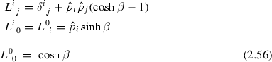
with \(\hat{\mathbf {p}}\,=\mathbf {p}/|\mathbf {p}|\), \(\cosh \beta =\omega _p/m\), \(\sinh \beta =|\mathbf {p}|/m\) and \(\tanh \beta =|\mathbf {p}|/\omega _p=v\) the velocity of the state.
- 10.
In \( SL (2,C)~\)the Lie algebra obviously has the \(2 \times 2\) matrix representation \(J_i=\sigma _i/2,\,K_i=\pm \text {i}~\sigma _i/2 \) in terms of the Pauli matrices, however, \(\mathbf {K}^+=-\mathbf {K}\) is non–Hermitian and the corresponding finite dimensional representation non–unitary. Unitary representations of the Lorentz group, required to implement relativistic covariance on the Hilbert space of physical states, are necessarily infinite dimensional. Actually, the two possible signs of \(K_i\) indicated exhibits that there are two different inequivalent representations.
- 11.
Again, these finite dimensional representations \(U_\varLambda \), \(U_P\) (below), etc. should not be confused with the corresponding infinite dimensional unitary representations \(U(\varLambda )\), U(P), etc. acting on the Hilbert space of physical states considered in the preceding section.
- 12.
Note that while \(P^2=1\) the phase \(\eta _P\) of its unitary representation \(U_P\) is constrained by \(U_P^2=\pm 1\) only, i.e. \(\eta _P= \pm 1\) or \(\pm \text {i}\).
- 13.
The standard representation of the Dirac field/algebra, described in Sect. 2.1.1, is adapted to a simple interpretation in the rest frame (requires \(m\ne 0\)). It may be obtained from the ones in the Weyl basis (“helicity” representation) by a similarity transformation \(\mathcal{S}\)
$$\begin{aligned}\psi (x) = \mathcal{S}\, \psi ^\mathrm {helicity} (x)~~,~~~\gamma _\mu = \mathcal{S}\,\gamma ^\mathrm {helicity}_\mu \mathcal{S}^{-1}~~ \,,\;~~~~ \mathcal{S}=\mathcal{S}^{-1}=\frac{1}{\sqrt{2}}\left( \begin{array}{rr} 1 &{} 1 \\ 1 &{} -1 \end{array} \right) \end{aligned}$$such that
$$\begin{aligned}u(0,r)=\sqrt{2m}\left( \begin{array}{c} U(r) \\ 0 \end{array} \right) \;,\;\;v(0,r)=\sqrt{2m}\left( \begin{array}{c} 0 \\ V(r) \end{array} \right) \end{aligned}$$in the standard basis.
- 14.
The known elementary particle interactions, the strong, electromagnetic and weak forces, all derive from a local gauge symmetry principle. This was first observed by Weyl [28] for the Abelian QED and later extended to non–Abelian gauge theories by Yang and Mills [29]. The gauge symmetry group governing the Standard Model of particle physics is \( SU (3)_c \otimes SU (2)_L \otimes U(1)_Y\).
- 15.
The modified derivative \(D_\mu =\partial _\mu -\text {i}e A_\mu (x)\) is called covariant derivative. e is the gauge coupling. The minimal substitution promotes the global gauge symmetry of the free Dirac Lagrangian to a local gauge symmetry of the electron–photon system, i.e., the interacting system has more symmetry than the free electron.
- 16.
The prescription \(: \cdots :\) means Wick ordering of products of fields: write the fields in terms of creation and annihilation operators and order them such that all annihilation operators are to the right of all creation operators, assuming the operators to commute (bosons) or to anticommute (fermions). This makes the vacuum expectation value of the field product vanish.
- 17.
The parametrization of the gauge dependence by the inverse of the Lagrange multiplier \(\xi =1/\lambda \) is just a commonly accepted convention.
- 18.
The mathematical problems with the point–like structure of elementary particles and with covariant quantization of the photons hindered the development of QFT for a long time until the break through at the end of the 1940s [34]. In 1965 Tomonaga, Schwinger and Feynman were honored with the Nobel Prize “for their fundamental work in quantum electrodynamics, with deep–ploughing consequences for the physics of elementary particles”. For non–Abelian gauge theories like the modern strong interaction theory Quantum Chromodynamics (QCD) [35, 36] and the electroweak Standard Model [37], the proper quantization, regularization and renormalization was another obstacle which was solved only at the beginning of the 1970 s by’t Hooft and Veltman [38]. They were awarded the Nobel Prize in 1999 “for elucidating the quantum structure of electroweak interactions in physics”. They have placed particle physics theory on a firmer mathematical foundation. They have in particular shown how the theory, beyond QED, may be used for precise calculations of physical quantities. Needless to say that these developments were crucial for putting precision physics, like the one with the anomalous magnetic moments, on a fundamental basis.
- 19.
Note that in QCD the corresponding closed quark loops with quark–gluon vertices behave differently because of the color matrices at each vertex. The trace of the product of color matrices in general has an even as well as an odd part.
- 20.
Diagrams which cannot be cut into two disconnected diagrams by cutting a single line. 1PI diagrams are the building blocks from which any diagram may be obtained as a tree of 1PI “blobs”.
- 21.
Often one simply chooses a cut–off (upper integration limit in momentum space) to make the integrals converge by “brute force”. A cut–off may be considered to parametrize our ignorance about physics at very high momentum or energy. If the cut–off \(\varLambda \) is large with respect to the energy scale E of a phenomenon considered, \(E\ll \varLambda \), the cut–off dependence may be removed by considering only relations between low–energy quantities (renormalization). Alternatively, a cut–off may be interpreted as the scale where one expects new physics to enter and it may serve to investigate how a quantity (or the theory) behaves under changes of the cut–off (renormalization group). In most cases simple cut–off regularization violates symmetries badly and it becomes a difficult task to make sure that one obtains the right theory when the cut–off is removed by taking the limit \(\varLambda \rightarrow \infty \) after renormalization.
- 22.
An inconsistency problem, concerning the definition of \(\gamma _5\) for \(d\ne 4\), implies that the chiral WT identities associated with the parity violating weak fermion currents in the SM are violated in general (see e.g. [45]).
- 23.
The dimension of \(F^{\mu \nu }\) is 2, 1 for the photon field plus 1 for the derivative.
- 24.
According to (2.122) there are two more potentially divergent structures
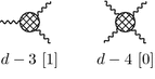
with superficial degree of divergence as indicated. However, the triple photon vertex is identically zero by Furry’s theorem, C odd amplitudes are zero in the C preserving QED. The four photon light–by–light scattering amplitude, due the transversality of the external physical photons, has an effective dimension \(d(\varGamma )_\mathrm {eff}=-4\), instead of 0, and is thus very well convergent. For the same reason, transversality of the photon self–energy, actually the photon propagator has \(d(\varGamma )_\mathrm {eff}=0\) instead of 2. In both cases it is the Abelian gauge symmetry which makes integrals better convergent than they look like by naive power counting.
- 25.
Note that because of the positivity of \(\mathbf {q}^{\,2}+m^2\) for any non–vacuum state, we have \(\omega _p-\text {i}\varepsilon =\sqrt{\mathbf {q}^{\,2}+m^2-\text {i}\varepsilon }\) in the limit \(\lim _{\varepsilon \rightarrow 0}\), which is always understood. The symbolic parameter \(\varepsilon \) of the \(\text {i}\varepsilon \) prescription, may be scaled by any fixed positive number.
- 26.
A direct integration here yields
$$m^2 (4 \pi ) ^{-d/2} \varGamma (1 - d/2) \left( \frac{m^2 }{ \mu ^2} \right) ^{d/2 - 2}$$which by virtue of \(\varGamma (1-d/2)=-2\varGamma (2-d/2)/(d-2)\) is the same analytic function as the one obtained via the partial integration method.
- 27.
Fermion propagators are represented either as an inverse matrix \(\frac{1}{{\not {k}}-m+\text {i}\varepsilon }\) or as a matrix \(\frac{\not {k}+m-\text {i}\varepsilon }{k^2-m^2+\text {i}\varepsilon }\) with a scalar denominator. This second form is obtained from the first one by multiplying numerator and denominator from the left or from the right with \(\not \!k+m-\text {i}\varepsilon \). In the denominator we then have \((\not \!k+m-\text {i}\varepsilon )(\not \!k-m+\text {i}\varepsilon )=\not \!k\not \!k-(m-\text {i}\varepsilon )^2 =k^2-m^2+\text {i}\varepsilon + O(\varepsilon ^2)\) where the \(O(\varepsilon ^2)\) order term as well as the \(O(\varepsilon )\) in the numerator in \(\varepsilon \) may be dropped as the limit \(\varepsilon \rightarrow 0\) is always understood.
- 28.
We adopt the scheme setting the trace of the unit matrix in spinor space \(\text {Tr}\,\mathbf {1}=4\); it is of course mandatory to keep this convention consistently everywhere. While bare quantities obviously depend on this convention, one can prove that quantities finite in the limit \(d \rightarrow 4\), like the renormalized ones, are unambiguous.
- 29.
As a rule, a cut diagram

contributes to the imaginary part if the cut diagram kinematically allows physical intermediate states: \(q^2\ge (m_1+m_2)^2\). In place of the virtual photon (a real photon requires \(q^2=0\) and does not decay) let us consider the massive charged weak gauge boson W. The W is an unstable particle and decays predominantly as \(W^- \rightarrow \ell ^- \bar{\nu }_\ell \) (\(\ell =e,\mu ,\tau \)) leptonically, and \(W^- \rightarrow d\bar{u},b\bar{c}\) hadronically. Looking at the transversal self–energy function \(\varPi _W (q^2)\) of the W on the mass shell \(q^2=M_W^2\) we have
$$\begin{aligned}\text {Im} \,\; \varPi _W (q^2=M_W^2)= M_W \; \varGamma _W \ne 0 \end{aligned}$$defining the finite width \(\varGamma _W\) of the W–particle. Note that \(W^- \rightarrow b\bar{t}\) is not allowed kinematically because the top quark t is heavier than the W (\(M_W= 80.385\pm 0.015\,\text {GeV}, m_t=173.21\pm 0.87\,\text {GeV}, m_b=4.18\pm 0.03\,\text {GeV}\)) for an on–shell W and hence does not contribute to the width.
Cutting lines means applying the substitution (see (2.141))
$$\begin{aligned}\frac{1}{p^2-m^2+\text {i}\varepsilon } \rightarrow -\text {i}\,\pi \,\delta (p^2-m^2) \end{aligned}$$for the corresponding propagators. In general the imaginary part is given by cutting sets of lines of a diagram in all possible ways such that the diagram is cut into two disconnected parts. A cut contributes if the cut lines can be viewed as external lines of a real physical subprocess. Note that the imaginary part of an n–loop amplitude is given by cut diagrams exhibiting \(n-1\) closed loops at most. The imaginary part therefore is less UV divergent in general. In particular, the imaginary part of a one–loop diagram is always finite.
- 30.
Which derives from
$$\begin{aligned}B_0(m,m;q^2)=\text {Reg}-\ln m^2 -\int _0^1 \text {d}z\,\ln (1-z\,(1-z)\,q^2/m^2) \end{aligned}$$(see (2.146)). The second form is obtained from the first one by a transformation of variables \(z \rightarrow t=2z-1\), noting that \( \int _0^1 \text {d}z\, \cdots = 2 \int _{\frac{1}{2}}^{1}\text {d}z\, \cdots \), and performing a partial integration with respect to the factor \(z\,(1-z)=(1-t^2)/4= \frac{\text {d}}{\text {d}t}\,t\,(1-t^2/3)/4\) in front of the logarithm.
- 31.
In the unbroken phase of the SM the left–handed and the right–handed fermion fields get renormalized independently by c–number renormalization factors \(\sqrt{Z_L}\) and \(\sqrt{Z_R}\), respectively. In the broken phase, a Dirac field is renormalized by \(\sqrt{Z_f}=\sqrt{Z_L}\,\varPi _-+\sqrt{Z_R}\,\varPi _+\) where \(\varPi _\pm =\frac{1}{2}(1\pm \gamma _5)\) are the chiral projectors. Hence, the wave function renormalization factor, becomes a matrix \(\sqrt{Z_f}=1+\alpha +\beta \gamma _5\) and the bare fields are related to the renormalized one’s by \(\psi _0(x) =\sqrt{Z_f} \psi _r(x)\), which for the adjoint field reads \(\bar{\psi }_0(x) = \bar{\psi }_r(x) \gamma ^0 \sqrt{Z_f} \gamma ^0\).
- 32.
We consider the photon to have a tiny mass and thus work with a photon propagator of the form

- 33.
Note that with \(T_2\) from (2.194) we have
$$\begin{aligned}\varSigma ^{\xi \ne 1}=\text {i}e^2 T_2=(\not \!p-m)\, A^{\xi \ne 1} \end{aligned}$$where
$$\begin{aligned}A^{\xi \ne 1}=(1-\xi )\, \frac{e^2}{16 \pi ^2} \, B_0(m_\gamma ,\sqrt{\xi }m_\gamma ;0) \end{aligned}$$and \(B^{\xi \ne 1}=-A^{\xi \ne 1}\), such that \(A^{\xi \ne 1}+B^{\xi \ne 1}=0\). This leads to a contribution
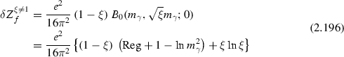
to the wave function renormalization.
- 34.
The Spence function is an analytic function with the same cut as the logarithm. Useful relations are
For \(|x|\le 1\) it has a series expansion
$$\begin{aligned}\mathrm {Sp} (x)=\sum \limits _{k=1}^{\infty } \frac{x^k}{k^2} \;.\\ \end{aligned}$$Special values are:
$$\begin{aligned}\mathrm {Sp} (0)=0 \;,\;\;\mathrm {Sp} (1)=\frac{\pi ^2}{6} \;,\;\;\mathrm {Sp} (-1)= -\frac{\pi ^2}{12} \;,\;\;\mathrm {Sp} ( \frac{1}{2}) = \frac{\pi ^2}{12}-\frac{1}{2}(\ln 2)^2 \;.\end{aligned}$$.
- 35.
One also may check this directly on the level of the standard scalar integrals \(A_0\), \(B_0\) and \(C_0\). Denoting by \(AA(m)=A_0(m)/m^2\) we have
$$\begin{aligned}\delta F_\mathrm {E}(q^2)&\mathop {\sim }\limits ^{q^2 \rightarrow 0} \propto \bigl ( [-4m^2C_0-3B_0(m,m;0)+4B_0(0,m;m^2)-2]_{A_1} \\&+\,[B_0(m,m;0)-B_0(0,m;m^2)]_{A_2} +[1+AA(m)+4m^2\dot{B}_0(m_\gamma ,m;m^2)]_{\delta Z_e} \bigr ) \;.\end{aligned}$$Using the relations
$$\begin{aligned}\begin{array}{lcl} C_0(m_\gamma ,m,m;m^2,0,m^2)&{}=&{} \frac{-1}{4m^2}\left( B_0(0,m;m^2)-1-AA(m)+2AA(m_\gamma )\right) \\ B_0(m,m;0)&{}=&{}-1 -AA(m)\\ B_0(0,m;m^2)&{}=&{}1-AA(m)\\ m^2\dot{B}_0(m_\gamma ,m;m^2)&{}=&{}-1-\frac{1}{2}AA(m_\gamma )+ \frac{1}{2}AA(m) \end{array} \end{aligned}$$one easily finds that indeed \(\delta F_\mathrm {E}(q^2) \mathop {\sim }\limits ^{q^2 \rightarrow 0} 0\). This kind of approach is usually utilized when working with computer algebra methods.
- 36.
The following example (electrons \(=\) full lines and photons \(=\) wavy lines) may illustrate this: fat lines carry the flow of large momentum (subgraph H)
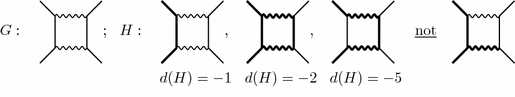
The first graph in the set H determines the leading behavior \(\mathcal{O}(\lambda ^{-1} \ln ^x \lambda )\). Note that all subgraphs H are connected and have no dead end lines (like the last diagram above, which is not a subgraph in the sense the term is used here). Thin lines attached to vertices of a subgraph H figure as external lines \(\mathcal{E}'\), such that \(\mathcal{E}_H=\mathcal{E}_\infty +\mathcal{E}'\) is the set of all external lines of H and \(d(H)=4-\frac{3}{2}f(\mathcal{E}_H)-b(\mathcal{E}_H)\).
- 37.
This latter restriction takes into account the decoupling of heavy flavors, valid in QED and QCD. Since in the \(\overline{\mathrm {MS}}\) scheme, i.e., renormalization by the substitution \(\text {Reg}\rightarrow \ln \mu ^2\), which we are considering here, decoupling is not automatic, one has to impose it by hand. At a given scale one is thus considering an effective theory, which includes only those particles with masses below the scale \(\mu \).
- 38.
In the scattering region the result is more complicated, because, there is one more kinematic variable, the scattering angle \(\varTheta \), or equivalently, the electron velocity \(\beta _e\). Considering, elastic scattering \(|\mathbf {p}_1|=|\mathbf {p}_2|\), \(E_1=E_2\) the finite function \(F'(y)\), now for \(y<0\) (\(0<\upxi <1\)), reads
$$\begin{aligned}F'(y)=\frac{1}{\sqrt{1-y}} \biggl \{- & {} \mathrm {Sp} \left( 1+\frac{2}{1+\upxi }\frac{1}{1-\beta _e}\right) -\mathrm {Sp} \left( 1+\frac{2}{1+\upxi }\frac{1}{1+\beta _e}\right) \\+ & {} \mathrm {Sp} \left( 1+\frac{2\upxi }{1+\upxi }\frac{1}{1-\beta _e}\right) +\mathrm {Sp} \left( 1+\frac{2\upxi }{1+\upxi }\frac{1}{1+\beta _e}\right) \biggr \} \end{aligned}$$where \(\beta _e=\sqrt{1-4m^2/s}\) is the velocity of the electron. s and \(Q^2=-q^2>0\) are related by \(Q^2=s\,\frac{1-\cos \varTheta }{2}\). The asymptotic behavior \(Q^2 \gg m^2\) at fixed angle requires \(s \gg m^2\) with \(r \equiv Q^2/s=(1-\cos \varTheta )/2\) fixed. The arguments of the Spence functions behave like \(1+\frac{2}{1+\upxi }\frac{1}{1-\beta _e}\simeq \frac{s}{m^2}- r^{-1}+\cdots \), \(1+\frac{2}{1+\upxi }\frac{1}{1+\beta _e}\simeq 2-\frac{m^2}{Q^2}+\frac{m^2}{s}+\cdots \), \(1+\frac{2\upxi }{1+\upxi }\frac{1}{1-\beta _e}\simeq 1+r^{-1} -(1+3r^{-1}) \frac{m^2}{Q^2}+\cdots \), and \(1+\frac{2\upxi }{1+\upxi }\frac{1}{1+\beta _e}\simeq 1+\frac{m^2}{Q^2}+\cdots \). Utilizing the relations (2.207), one may work out the leading behavior
$$\begin{aligned}C^\mathrm {scattering}_\mathrm {bre}=\frac{\alpha }{\pi } \left\{ 2\ln \frac{Q^2}{m^2}\ln \frac{2\omega }{m_\gamma } -\frac{1}{2}\ln ^2 \frac{s}{m^2}-2 \ln \frac{2\omega }{m_\gamma } + \ln \frac{Q^2}{m^2} +\cdots \right\} \end{aligned}$$which, with \(\ln ^2 s/m^2 =-\ln ^2 Q^2/m^2+2\ln Q^2/m^2 \ln s/m^2 +\ln ^2 s/Q^2\) and after neglecting the last (sub leading) term, is in agreement with [2]. In the production channel with \(q^2=-Q^2>0\), in the center of mass frame of the produced lepton pair, the leptons are back–to–back and hence \(\varTheta =\pi \), or \(\cos \varTheta =-1\), such that s may be identified as \(s=q^2\).
- 39.
The factorization into \(e^+e^-\rightarrow \gamma ^*\) production and subsequent decay \(\gamma ^* \rightarrow \ell ^+ \ell ^-\) only makes sense at relatively low \(q^2\), when the one–photon exchange approximation can be used. In the SM the \(\gamma ^*\) may also be a “heavy light” particle Z of mass about \(M_Z \simeq 91\,\text {GeV}\) which is unstable and thus is described well by a Breit–Wigner resonance. Near the resonance energy again factorization is an excellent approximation and the following discussion applies. In \(e^+e^-\)–annihilation, the radiation of additional photons from the initial state electron or positron (Fig. 2.11 with \(e'\) an incoming \(e^+\)) is called initial state radiation (ISR). In the soft approximation (2.243) still holds. For details see (5.11) in Sect. 5.1.3.
- 40.
The limits \(m_\gamma ^2 \rightarrow 0\) for \(p^2=m^2\) and \(\mu ^2=m^2-p^2 \rightarrow 0\) for \(m_\gamma ^2=0\) coincide upon identifying \(\mu ^2=m\, m_\gamma \) at least in one-loop calculations.
- 41.
i.e. particle number conserving, when looked at from the crossed t-channel \(e^- \mu ^+ \rightarrow e^- \mu ^+\).
- 42.
This basically says that diagrams that destroy the initial quark and antiquark are strongly suppressed with respect to those that do not. As an example, while \(\phi \rightarrow \pi ^+\pi ^-\) is “Zweig” forbidden, \(\rho ^0 \rightarrow \pi ^+\pi ^-\) is allowed.


References
J.D. Bjorken, S.D. Drell, Relativistic Quantum Mechanics, 1st edn. (McGraw-Hill, New York 1964), 300 p; Relativistic Quantum Fields, 1st edn. (McGraw-Hill, New York, 1965), 396 p
V.B. Berestetskii, E.M. Lifshitz, L.P. Pitaevskii, Quantum electrodynamics, Landau and Lifshitz Course of Theoretical Physics, vol. 4, 2nd edn. (Pergamon, London, 1982), 652 p
P.A.M. Dirac, Proc. R. Soc. A 114, 243 (1927); Proc. R. Soc. A 126, 360 (1930); Proc. R. Soc. A 136, 453 (1932)
E.P. Wigner, Ann. Math. 40, 149 (1939)
P. Jordan, E.P. Wigner, Zeits. Phys. 47, 631 (1928)
W. Heisenberg, W. Pauli, Zeits. Phys. 56, 1 (1929); Zeits. Phys. 59, 168 (1930); P.A.M. Dirac, V.A. Fock, B. Podolsky, Phys. Zeits. Sowjetunion 3, 64 (1932)
H. Joos, Fortsch. Phys. 10, 65 (1962); S. Weinberg, Phys. Rev. 133, B1318 (1964); Phys. Rev. 134, B882 (1964)
P.A.M. Dirac, Proc. R. Soc. A 114, 243 (1927); A 117, 610 (1928)
W. Pauli, Zeits. Physik 31, 765 (1925)
W. Pauli, Phys. Rev. 58, 716 (1940)
R.F. Streater, A.S. Wightman, CPT, Spin and Statistics and All That (Benjamin, New York, 1964)
G. Lüders, K. Danske Vidensk, Selsk. Mat.-Fys. Medd. 28(5) (1954); W. Pauli, Exclusion principle, Lorentz group and reflection of space-time and charge, in Niels Bohr and the Development of Physics, ed. by W. Pauli (Pergamon Press, London, 1955, reissued 1962), pp. 30–51; W. Pauli, II Nuovo Cim. 6, 204 (1957); G. Lüders, Ann. Phys. N. Y. 2, 1 (1957); G. Lüders, B. Zumino, Phys. Rev. 106, 345 (1957); R. Jost, Helv. Phys. Acta 30, 409 (1957)
S. Gasiorovicz, Elementary Particle Physics (Wiley, New York, 1966)
S. Eidelman et al. [Particle Data Group], Phys. Lett. B 592, 1 (2004); K.A. Olive et al. [Particle Data Group], Chin. Phys. C 38, 090001 (2014) and 2015 update
B.C. Regan, E.D. Commins, C.J. Schmidt, D. DeMille, Phys. Rev. Lett. 88, 071805 (2002)
J. Baron et al. [ACME Collab.], Science 343, 269 (2014)
W. Gerlach, O. Stern, Zeits. Physik 8, 110 (1924)
R. Kronig (1925 unpublished), https://en.wikipedia.org/wiki/Ralph_Kronig
G.E. Uhlenbeck, S. Goudsmit, Naturwissenschaften 13, 953 (1925); Nature 117, 264 (1926)
W. Pauli, Zeits. Phys. 43, 601 (1927)
F. Englert, R. Brout, Phys. Rev. Lett. 13, 321 (1964)
P.W. Higgs, Phys. Lett. 12, 132 (1964)
G. Aad et al. [ATLAS Collab.], Phys. Lett. B 716, 1 (2012); Science 338, 1576 (2012)
S. Chatrchyan et al. [CMS Collab.], Phys. Lett. B 716, 30 (2012); Science 338, 1569 (2012)
S. Weinberg, Phys. Rev. 134, B882 (1964)
R. Frisch, O. Stern, Zeits. Physik 85, 4 (1933); I. Estermann, O. Stern, ibid. 85, 17 (1933)
G. Charpak, F.J.M. Farley, R.L. Garwin, T. Muller, J.C. Sens, A. Zichichi, Phys. Lett. 1B, 16 (1962)
H. Weyl, Zeits. Phys. 56, 330 (1929)
C.N. Yang, R.L. Mills, Phys. Rev. 96, 191 (1954)
M. Gell-Mann, F. Low, Phys. Rev. 95, 1300 (1954)
G.C. Wick, Phys. Rev. 80, 268 (1950)
W. Pauli, F. Villars, Rev. Mod. Phys. 21, 434 (1949)
N.N. Bogoliubov, D.V. Shirkov, Introduction to the Theory of Quantized Fields, 1st & 2nd edn. (Wiley, New York, 1957, 1980), 720 p
S. Tomonaga, R. Iho, Progr. Theor. Phys. 1, 27 (1946); J. Schwinger, Phys. Rev. 74, 1439 (1948); R.P. Feynman, Phys. Rev. 76, 749 (1949); F. Dyson, Phys. Rev. 75, 486 (1949), ibid. 1736
H. Fritzsch, M. Gell-Mann, H. Leutwyler, Phys. Lett. 47B, 365 (1973)
H.D. Politzer, Phys. Rev. Lett. 30, 1346 (1973); D. Gross, F. Wilczek, Phys. Rev. Lett. 30, 1343 (1973)
S.L. Glashow, Nucl. Phys. B 22, 579 (1961); S. Weinberg, Phys. Rev. Lett. 19, 1264 (1967); A. Salam, Weak and electromagnetic interactions, in Elementary Particle Theory, ed. by N. Svartholm (Amquist and Wiksells, Stockholm, 1969), pp. 367–377
G. ’t Hooft, Nucl. Phys. B 33, 173 (1971); 35, 167 (1971); G. ’t Hooft, M. Veltman, Nucl. Phys. B 50, 318 (1972)
G. t’ Hooft, M. Veltman, Nucl. Phys. B 44, 189 (1972)
W.H. Furry, Phys. Rev. 51, 125 (1937)
F. Dyson, Phys. Rev. 75, 1736 (1949); J.S. Schwinger, Proc. Nat. Acad. Sci. 37, 452–459 (1951)
H. Lehmann, K. Symanzik, W. Zimmermann, Nuovo Cim. 1, 205 (1955); Nuovo Cim. 6, 319 (1957)
S. Mandelstam, Phys. Rev. 112, 1344 (1958)
I. Białynicki-Birula, Phys. Rev. D 2, 2877 (1970)
F. Jegerlehner, Eur. Phys. J. C 18, 673 (2001)
D. Akyeampong, R. Delbourgo, Nuovo Cim. 17A, 47 (1973); W.A. Bardeen, R. Gastmans, B. Lautrup, Nucl. Phys. B 46, 319 (1972); M. Chanowitz, M. Furman, I. Hinchliffe, Nucl. Phys. B 159, 225 (1979)
M.C. Bergère, F. David, J. Math. Phys. 20, 1244 (1979)
K. Osterwalder, R. Schrader, Commun. Math. Phys. 31, 83 (1973); ibid. 42, 281 (1975)
K.G. Wilson, Phys. Rev. D 10, 2445 (1974)
M. Abramowitz, I. Stegun, Handbook of Mathematical Functions (Dover, New York, 1965) (Chap. 9 and formulas 9.1.39/9.1.40/9.6.4 there)
I.S. Gradshteyn, I.M. Ryzhik, Table of Integrals, Series, and Products, eds. by A. Jeffery, D. Zwanziger (Academic Press, London, 2015[1943]) (Formulas 3.471.9/11)
G. t’Hooft, M. Veltman, Nucl. Phys. B 153, 365 (1979)
A.I. Davydychev, M.Y. Kalmykov, Nucl. Phys. B 605, 266 (2001)
J. Fleischer, F. Jegerlehner, O.V. Tarasov, Nucl. Phys. B 672, 303 (2003)
J.S. Frederiksen, W.S. Woolcock, Nucl. Phys. B 28, 605 (1971); Aust. J. Phys. 26, 691 (1973); Ann. Phys. 75, 503 (1973); ibid. 80, 86 (1973)
G. Passarino, M. Veltman, Nucl. Phys. B 160, 151 (1979)
K.G. Chetyrkin, F.V. Tkachov, Nucl. Phys. B 192, 159 (1981)
F. Jegerlehner, Renormalizing the standard model, in Testing the Standard Model, eds. by M. Cvetič, P. Langacker (World Scientific, Singapore, 1991), pp. 476–590, http://www-com.physik.hu-berlin.de/~fjeger/books.html
F. Bloch, A. Nordsieck, Phys. Rev. D 52, 54 (1937)
Y. Hahn, W. Zimmermann, Commun. Math. Phys. 10, 330 (1968); W. Zimmermann, Commun. Math. Phys. 11, 1 (1968); J.H. Lowenstein, W. Zimmermann, Commun. Math. Phys. 44, 73 (1975)
F.J. Dyson, Phys. Rev. 75, 1736 (1949)
J.P. Fink, J. Math. Phys. 9, 1389 (1968); E.B. Manoukian, J. Math. Phys. 19, 917 (1978)
S. Weinberg, Phys. Rev. 118, 838 (1960)
T. Appelquist, J. Carazzone, Phys. Rev. D 11, 2856 (1975)
V.A. Smirnov, Mod. Phys. Lett. A 10, 1485 (1995) (and references therein)
E.C.G. Stueckelberg, A. Petermann, Helv. Phys. Acta 26, 499 (1953); M. Gell-Mann, F.E. Low, Phys. Rev. 95, 1300 (1954)
G. Mack, Nucl. Phys. B 5, 499 (1968)
J.D. Bjorken, Phys. Rev. 179, 1547 (1969); J.D. Bjorken, E.A. Paschos, Phys. Rev. 185, 1975 (1969)
D.H. Coward et al., Phys. Rev. Lett. 20, 292 (1968); E.D. Bloom et al., Phys. Rev. Lett. 23, 930 (1969); G. Miller et al., Phys. Rev. D 5, 528 (1972)
H. Suura, E. Wichmann, Phys. Rev. 105, 1930 (1957); A. Petermann, Phys. Rev. 105, 1931 (1957)
B.E. Lautrup, E. de Rafael, Nucl. Phys. B 70, 317 (1974)
E. de Rafael, J.L. Rosner, Ann. Phys. (N.Y.) 82, 369 (1974)
A.L. Kataev, S.A. Larin, Pisma Zh. Eksp. Teor. Fiz. 96, 64 (2012) [JETP Lett. 96, 61 (2012)]
P.A. Baikov, K.G. Chetyrkin, J.H. Kühn, C. Sturm, Nucl. Phys. B 867, 182 (2013)
P.A. Baikov, K.G. Chetyrkin, J.H. Kühn, J. Rittinger, JHEP 1207, 017 (2012)
D.R. Yennie, S.C. Frautschi, H. Suura, Ann. Phys. 13, 379 (1961); D.R. Yennie, Phys. Lett. 34B, 239 (1975); J.D. Jackson, D.L. Scharre, Nucl. Instr. 128, 13 (1975); M. Greco, G. Pancheri, Y. Srivastava, Nucl. Phys. B 101, 234 (1975)
T. Kinoshita, J. Math. Phys. 3, 650 (1962); T.D. Lee, M. Nauenberg, Phys. Rev. D 133, B1549 (1964)
J. Fleischer, F. Jegerlehner, Z. Phys. C 26, 629 (1985)
G. Sterman, S. Weinberg, Phys. Rev. Lett. 39, 1436 (1977)
O. Steinmann, Commun. Math. Phys. 237, 181 (2003)
F. Jegerlehner, Nucl. Phys. B (Proc. Suppl.) 51C, 131 (1996)
G.J. Gounaris, J.J. Sakurai, Phys. Rev. Lett. 21, 244 (1968); A. Quenzer et al., Phys. Lett. B 76, 512 (1978)
F. Jegerlehner, R. Szafron, Eur. Phys. J. C 71, 1632 (2011)
H. Leutwyler, Electromagnetic form factor of the pion, in Continuous Advances in QCD 2002: Proceedings, eds. by K.A. Olive, M.A. Shifman, M.B. Voloshin (World Scientific, Singapore, 2002), 646 p, arXiv:hep-ph/0212324
J. Gasser, H. Leutwyler, Ann. Phys. 158, 142 (1984); Nucl. Phys. B 250, 465 (1985)
K.G. Wilson, Phys. Rev. D 10, 2445 (1974); M. Creutz, Phys. Rev. D 21, 2308 (1980)
Y. Nambu, Phys. Rev. Lett. 4, 380 (1960)
G. ’t Hooft, Nucl. Phys. B 72, 461 (1974); ibid. 75, 461 (1974); E. Witten, Nucl. Phys. B 160, 57 (1979)
A.V. Manohar, Hadrons in the \(1/N\) expansion, in At the frontier of Particle Physics, vol. 1, ed. M. Shifman (World Scientific, Singapore, 2001)pp. 507–568
H. Leutwyler, Nucl. Phys. Proc. Suppl. 64, 223 (1998); R. Kaiser, H. Leutwyler, Eur. Phys. J. C 17, 623 (2000)
S. Okubo, Phys. Lett. 5, 1975 (1963); G. Zweig, CERN Report No.8419/TH412 (1964); J. Iizuka. Prog. Theor. Phys. Suppl. 37, 38 (1966)
S.L. Glashow, Phys. Rev. Lett. 7, 469 (1961)
S. Okubo, Phys. Lett. 5, 165 (1963)
W.E. Caswell, Phys. Rev. Lett. 33, 244 (1974); D.R.T. Jones, Nucl. Phys. B 75, 531 (1974); E. Egorian, O.V. Tarasov, Theor. Math. Phys. 41, 863 (1979) [Teor. Mat. Fiz. 41, 26 (1979)]
O.V. Tarasov, A.A. Vladimirov, A.Y. Zharkov, Phys. Lett. B 93, 429 (1980); S.A. Larin, J.A.M. Vermaseren, Phys. Lett. B 303, 334 (1993)
T. van Ritbergen, J.A.M. Vermaseren, S.A. Larin, Phys. Lett. B 400, 379 (1997); M. Czakon, Nucl. Phys. B 710, 485 (2005); K.G. Chetyrkin, Nucl. Phys. B 710, 499 (2005)
P.A. Baikov, K.G. Chetyrkin, J.H. Kühn, Phys. Rev. Lett. 118, 082002 (2017)
S. Bethke, Phys. Rep. 403–404, 203 (2004)
K.A. Olive et al. (Particle Data Group), Chin. Phys. C 38, 090001 (2014); Quantum Chromodynamics eds. by S. Bethke, G. Dissertori, G.P. Salam (therein)
M. Della Morte, R. Frezzotti, J. Heitger, J. Rolf, R. Sommer, U. Wolff, Nucl. Phys. B 713, 378 (2005)
F. Tekin et al. [ALPHA Collab.], Nucl. Phys. B 840, 114 (2010)
M. Dalla Brida et al. [ALPHA Collab.], Phys. Rev. D 95, 014507 (2017)
M. Bruno et al., Nucl. Part. Phys. Proc. 285–286, 132 (2016); PoS Lattice 2016, 197 (2016), arXiv:1701.03075 [hep-lat]
F. Jegerlehner, Acta Phys. Polon. B 45, 1167 (2014)
Author information
Authors and Affiliations
Corresponding author
Rights and permissions
Copyright information
© 2017 Springer International Publishing AG
About this chapter
Cite this chapter
Jegerlehner, F. (2017). Quantum Field Theory and Quantum Electrodynamics. In: The Anomalous Magnetic Moment of the Muon. Springer Tracts in Modern Physics, vol 274. Springer, Cham. https://doi.org/10.1007/978-3-319-63577-4_2
Download citation
DOI: https://doi.org/10.1007/978-3-319-63577-4_2
Published:
Publisher Name: Springer, Cham
Print ISBN: 978-3-319-63575-0
Online ISBN: 978-3-319-63577-4
eBook Packages: Physics and AstronomyPhysics and Astronomy (R0)