An Introduction to Algebras of Chiral Differential Operators

Abstract

These notes are an informal introduction to algebras of chiral differential operators. The language used is one of vertex algebras, otherwise the approach chosen is that suggested by Beilinson and Drinfeld. The prerequisites are kept to a minimum, and we even give an informal introduction to the Beilinson-Bernstein localization theory in the example of the projective line.

Partially supported by an NSF grant.

1 Introduction

These lectures are an informal introduction to algebras of chiral differential operators, the concept that was independently and at about the same time discovered in [25] and, in a significantly greater generality, in [7]. The key to these algebras is the notion of a chiral algebroid, which is a vertex algebra analogue of the notion of a Picard-Lie algebroid. In the context of vertex algebras it was put forward in [17]; in these notes, however, despite the relentless focus on vertex algebras instead of various pseudo-tensor categories, we shall follow a much more natural approach of [7]. Under the assumption that the algebras in question are conformally graded, the results we obtain are the same as in [17].

As a warm-up, we spend considerable time discussing ordinary (and twisted) algebras of differential operators, going so far as to prove parts of the Bernstein-Beilinson localization theory in the case of sl₂. We hope this will create the framework within which things vertex will make more sense.

A little Lie and commutative algebra will suffice to understand much of what follows; dealing with the sheaves will require that the reader is not put off by some sheaf-theoretic and algebro-geometric terminology. Formally, no knowledge of vertex algebras is required, and the main definitions are all recorded, but in practice, without some such knowledge some of the sections below will be a tough read. On the other hand, these notes will supply the student studying books such as [11, 19] with a wealth of “real life examples.” A number of exercise is intended to enhance the reader’s experience.

The author would like to thank the organizers for the unforgettable fortnight in Pisa.

2 The Algebra of Differential Operators

For the purposes of these lectures, $\mathbb{C}$ is the ground field, A is a finitely generated commutative $\mathbb{C}$-algebra.

A linear transformation $P \in \text{End}_{\mathbb{C}}(A)$ is called a differential operator of order k if k is the least integer s.t. [ f _k+1, […[ f ₂, [ f ₁, P]…] = 0 for all f ₁, …, f _k+1 ∈ A. Here f ∈ A means the operator of multiplication by f and [X, Y ] = X ∘ Y − Y ∘ X.

Let D _A ^(k) be the space of all differential operators of order at most k.

Exercise 2.1

• (i) The map

  

  is an algebra isomorphism.

• (ii) Let $T_{A} =\{ P \in \text{End}_{\mathbb{C}}(A)\text{ s.t. }P(ab) = P(a)b + aP(b)\}$. One has .

• (iii) Furthermore, there is a split exact sequence

  

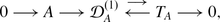  (1)

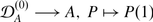
  with defined by P ↦ [P, . ], where [P, . ] stands for the map A ⟶ A, a ↦ [P, a]. Hence, , canonically.

• (iv) .

• (v) .

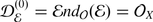
Define . The assertions of the exercise show that is an associative (unital) filtered algebra; the corresponding graded object, , is an associative commutative algebra. (Of course, we let .) Formula (1) and its various generalization will be the focus of our attention.

Now assume A is “smooth,” which we take to mean that the module of Kähler differentials, Ω _A ¹, is a finitely generated free A-module.

Lemma 2.1

There is an algebra isomorphism

where S _A ^• T _A is the symmetric algebra A ⊕ T _A ⊕ S _A ² T _A ⊕⋯ .

Proof

The fact that there is an isomorphism , which was discussed in page 74, furnishes the basis of induction, on the one hand, and gives an algebra map , on the other hand. Let us now define the inverse map. There is a map

It clearly descends to a map

Furthermore, its image actually belongs to the space of derivations, Der , which is the same as

. Thus we obtain a map

All of this is valid for any A, but if Ω _A is free, then we have an identification

Using the induction assumption we obtain

Exercise 2.2

The two maps constructed above,

are each other’s inverses. □

In particular, is generated by vector fields. This is not true in general.

Exercise 2.3

Let $A = \mathbb{C}[x]/(x^{n})$. Verify that , which by definition is a subalgebra of $gl(A) = gl_{n}(\mathbb{C})$, is actually isomorphic to $gl_{n}(\mathbb{C})$. Describe T _A and show it does not generate .

If A is smooth, then for any “point,” i.e. $\mathfrak{m} \in \text{Specm}(A)$, there are elements x ₁, …, x _n ∈ A s.t. the images of their differentials, dx ₁, …, dx _n , in the fiber $\varOmega _{A}/\mathfrak{m}\varOmega _{A}$ form a basis. Therefore, {dx ₁, …, dx _n } is a basis of the localization $\varOmega _{A_{f}}$ for some f ∈ A. Let {∂ ₁, …, ∂ _n } be the dual basis of $T_{A_{f}}$ s.t. dx _i (∂ _j ) = δ _ij . It follows that [∂ _i , ∂ _j ] = 0. One has , and so, locally, each differential operator can be written in the form familiar to the calculus student.

A Poisson algebra comprises two structures, one of a commutative associative algebra, another of Lie algebra, that are compatible in the sense that the operator of the Lie bracket with any fixed element, {a, . }, satisfies the Leibniz identity: {a, bc} = {a, b}c + a{b, c}.

If is a filtered associative algebra s.t. the graded object, , is a commutative algebra, then is naturally a Poisson algebra with the Lie bracket , where $\bar{a}$ ($\bar{b}$ resp.) is a class of ( resp.) In such a situation it is common to say that is a quantization of .

The commutative associative algebra S _A ^• T _A is naturally a Poisson algebra, the bracket being the Lie bracket on T _A extended as a derivation to the whole of S _A ^• T _A . If A is smooth, then by Lemma 2.1 and as such carries another, a priori different, Poisson structure. A moment’s thought will show that these two Poisson structure coincide. Hence is a quantization of S _A ^• T _A .

Algebras of differential operators localize well.

Lemma 2.2

If Ω _A is free of finite rank, then .

Proof

A differential operator over A defines a differential operator over localization A _f as the following recurrent procedure shows: if , write

$$\displaystyle{P(g) = P(\,f^{n} \frac{g} {f^{n}}) = f^{n}P( \frac{g} {f^{n}}) + [P,f^{n}]( \frac{g} {f^{n}}),}$$

then solve for $P( \frac{g} {f^{n}})$, which makes sense, since , and so $[P,f^{n}]( \frac{g} {f^{n}})$ may be assumed to be known.

This gives a map , which respects the natural filtrations; hence maps of graded objects (Lemma 2.1): $A_{f} \otimes _{A}S_{A}^{i}T_{A} \rightarrow S_{A_{f}}^{i}T_{A_{f}}$, $i\geqslant 1$. These are isomorphisms as follows from an obvious inductive argument, the basis of induction, i = 1, being the standard commutative algebra computation:

$$\displaystyle{T_{A_{f}}\mathop{\longrightarrow }\limits^{ \sim }\text{Hom}_{A_{f}}(\varOmega _{A_{f}},A_{f})\mathop{\longrightarrow }\limits^{ \sim }\text{Hom}_{A_{f}}(A_{f}\otimes _{A}\varOmega _{A},A_{f})\mathop{\longrightarrow }\limits^{ \sim } A_{f}\otimes _{A}\text{Hom}_{A}(\varOmega _{A},A)\mathop{\longrightarrow }\limits^{ \sim } A_{f}\otimes _{A}T_{A}.}$$

□

Smoothness is not essential for this result, finite generation is.

Exercise 2.4

• (i) Prove for any finitely generated algebra A.

• (ii) Find an example of A s.t. $T_{A_{f}}$ is not isomorphic to A _f ⊗ _A T _A .

It is now clear that each smooth algebraic variety X carries a sheaf of filtered associative algebras, , s.t. .

A Lie algebra $\mathfrak{g}$ gives rise to the universal enveloping algebra $U(\mathfrak{g})$. A similar construction reproduces . Namely, is isomorphic to the quotient of modulo the 2-sided ideal J generated by the elements , f ∗ g − fg, f ∗ ∂ − f∂; here and are the units in the respective algebras, , , and ∗ denotes the product in . Indeed, the universal property of gives a morphism that sends J to 0. Both algebras, and are filtered (use the Poincaré-Birkhof-Witt filtration on the former), and the morphism preserves the filtrations giving us the map . Lemma 2.1 shows that this map is an isomorphism.

An obvious analogous construction reproduces if A is the coordinate ring of a smooth affine variety.

To see what differential operators may be good for, outside PDE, let us consider the simplest case of the Beilinson-Bernstein localization [5, 6]. The Lie algebra of the group

$$\displaystyle{\text{SL}_{2} =\{ \left (\begin{array}{cc} a&b\\ c &d \end{array} \right ):\; ad-bc = 1,a,b,c,d \in \mathbb{C}\}}$$

is

$$\displaystyle{\text{sl}_{2} =\{ \left (\begin{array}{cc} a&b\\ c &d \end{array} \right ):\; a+d = 0,a,b,c,d \in \mathbb{C}\}\text{ with }[A,B] = AB-BC,}$$

the elements

$$\displaystyle{e = \left (\begin{array}{cc} 0&1\\ 0 &0 \end{array} \right ),\;h = \left (\begin{array}{cc} 1& 0\\ 0 & -1 \end{array} \right ),\;f = \left (\begin{array}{cc} 0&0\\ 1 &0 \end{array} \right )}$$

forming its basis.

The group tautologically operates on $\mathbb{C}^{2}$, hence on $\mathbb{C}\mathbb{P}^{1}$, the set of lines in $\mathbb{C}^{2}$. Therefore, there arises a Lie algebra morphism

which induces the associative algebra morphism

Exercise 2.5

• (i) Verify that on an appropriate chart $\mathbb{C}\hookrightarrow \mathbb{C}\mathbb{P}^{1}$, this morphism is defined by

  $$\displaystyle{e\mapsto - \frac{\partial } {\partial x},\;h\mapsto - 2x \frac{\partial } {\partial x},\;f\mapsto x^{2} \frac{\partial } {\partial x}.}$$

• (ii) Prove that the map sends the element ef + fe + h ²∕2 to 0.

The element ef + fe + h ²∕2 is, of course, the generator of the center of U(sl₂) (check at least that it is central!). Denote by U(sl₂)₀ the quotient U(sl₂)∕(ef + fe + h ²∕2)U(sl₂). We obtain the morphism

Lemma 2.3

This morphism is an isomorphism

Furthermore, if i > 0.

Proof

Both algebras at hand are filtered, and the map preserves filtrations; the passage to the graded object gives

(2)

We will prove the following two assertions: there are vector space isomorphisms

(3)

and

(4)

These assertions mean that (2) is an isomorphism, and the lemma follows.

Proof of (3) is a simple exercise on locally free sheaves over $\mathbb{C}\mathbb{P}^{1}$. is the Serre twisting sheaf , and so . The long exact cohomology sequence attached to the exact sequence

shows, by an obvious induction on n, that and

as desired.

Proof of (4) is, on the other hand, a pleasing exercise on some classic representation theory. Both sides of (4) are sl₂-modules: the adjoint action of sl₂ on U(sl₂) clearly descends to an action on the L.H.S; the action on the R.H.S is defined similarly using the morphism and the Lie bracket. This description shows that map (4) is an sl₂-module morphism. Kostant, [23], has computed the sl₂-module structure of $\text{Gr}U(\mathfrak{g})_{0}$ for any simple $\mathfrak{g}$. In our case, the result is

$$\displaystyle{ \text{Gr}U(\text{sl}_{2})_{0}\mathop{\longrightarrow }\limits^{ \sim }\bigoplus _{n=0}^{\infty }L_{ 2n}, }$$

(5)

which we shall prove a few lines below; here L _2n is the unique irreducible (2n + 1)-dimensional sl₂-module. Furthermore, L _2n ⊂ GrU(sl₂)₀ is generated by e ⁿ, the highest weight vector of highest weight 2n

On the right hand side, some elementary algebraic geometry will show that and that . Since (d∕dx)ⁿ is up to sign the image of e ⁿ (under ), this implies the desired isomorphism.

It remains to prove (5). It is clear that (ef + fe + h ²∕2)^m e ⁿ ∈ S ^•sl₂ generates an L _2n ⊂ S ^•sl₂. Furthermore, the set $\{(ef + fe + h^{2}/2)^{m}e^{n} \in S^{\bullet }\text{sl}_{2},\;m,n\geqslant 0\}$ is linearly independent. The complete reducibility of sl₂-modules implies that

$$\displaystyle{\bigoplus _{N=0}^{\infty }(\mathbb{C}[ef + fe + h^{2}/2] \otimes L_{ 2N})\hookrightarrow S^{\bullet }\text{sl}_{ 2}.}$$

Now one can show that both these spaces have the “same size.” To any bi-graded vectors space, V = ⊕ _m, n V _mn , we attach the formal character, chV = ∑ _mn dimV _mn x ^m t ⁿ. In our case, the first grading is the canonical grading of the symmetric algebra (s.t. the degree of x ∈ sl₂ is 1), the second is given by the eigenvalues of [h, . ]. For example, the reader will readily verify that

$$\displaystyle{chS^{\bullet }\text{sl}_{2} = \frac{1} {(1 - x^{2}t)(1 - t)(1 - x^{-2}t)},\;ch(1 \otimes L_{2n}) = t^{n}\frac{x^{2n+1} - x^{-2n-1}} {x - x^{-1}}.}$$

The following exercise will complete the proof of (5), hence of Lemma 2.3.

Exercise 2.6

Prove that¹

$$\displaystyle{ch(\bigoplus _{N=0}^{\infty }(\mathbb{C}[ef + fe + h^{2}/2] \otimes L_{ 2N})) = chS^{\bullet }\text{sl}_{ 2}.}$$

The very existence of a morphism implies there are two functors

The famous theorem of Beilinson-Bernstein [5] asserts that these are quasi-inverses of each other, Lemma 2.3 being an important step in the proof.

Examples-Exercises2.7

• (i) .

• (ii) , where is the structure sheaf=sheaf of regular functions, a tautological D-module.

• (iii) Let τ be the vector field that is the image of e ∈ sl ₂ under , and let $\infty \in \mathbb{C}\mathbb{P}^{1}$ be the (unique) point where τvanishes. Denote by the sheaf of functions that are allowed to have a pole at ∞, i.e., . Then , the contragradient Verma module with highest weight 0, that is, an appropriately defined dual of the Verma module M ₀ = U(sl ₂)∕U(sl ₂)〈h, e〉.

• (iv) With the notation of (iii), let be the ideal of ∞. Then is M ₋₂ = U(sl ₂)∕U(sl ₂)〈h + 2, e〉, the Verma module of highest weight -2. Notice that if y is a local coordinate s.t. $\mathfrak{m}_{\infty } = (y)$ , then and is thought of as the space of distributions supported at ∞.

• (v) An exact sequence of sheaves

  

  is transformed by Γ into the simplest example of the BGG resolution [ 18 , Chap. 6 ]:

  $$\displaystyle{0\longrightarrow \mathbb{C}\longrightarrow M_{0}^{c}\longrightarrow M_{ -2}\longrightarrow 0.}$$

At this point an obvious question arises: the L.H.S. of the Beilinson-Bernstein localization theorem, U(sl₂)₀, is a member of the family of algebras, U(sl₂) _χ = U(sl₂)∕U(sl₂)(ef + fe + h ²∕2 −χ), $\chi \in \mathbb{C}$.; is there an appropriate ? The answer is, yes, there is.

3 Algebras of Twisted Differential Operators

We shall begin with a class of examples.

Let X be an algebraic variety, a rk = 1 locally free sheaf of -modules (= the sheaf of sections of a rk = 1 complex vector bundle), the sheaf of linear transformations of . Define (cf. page 74) s.t.

and call it the sheaf of differential operators of order at most k operating on . The reader is invited to verify that our discussion of ordinary differential operators carries over to this case essentially intact as follows:

• (i) ; furthermore,

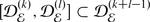
• (ii) .

• (iii) to assign the derivation , . Thus arising map

  

  is a surjective Lie algebra morphism. It defines an exact sequence

  

  (6)

  It is fundamentally different from (1) in that it does not split; having a splitting is equivalent to defining a connection on .

To summarize, defined to be is a sheaf of filtered algebras, locally isomorphic to ; this is because locally is indistinguishable from . If X is smooth then ; therefore is a quantization of (see page 76), usually not isomorphic to .

Exercise 3.1

If X is smooth, prove is Nötherian.

Let us now look at an example.

The routine verifications of all the assertions to follow is left to the reader.

$\mathbb{C}\mathbb{P}^{1}$ is covered by an atlas consisting of two charts, both $\mathbb{C}$ with coordinates x and y s.t. over the intersection, $\mathbb{C}^{{\ast}}$, x = 1∕y. Over each chart Serre’s twisting sheaf , which we have already encountered, is trivialized by sections s and t resp.; over the intersection s = y ⁿ t.

The trivializations identify with over each chart; we shall write ∇ _x for ∂∕∂x over the x-chart and ∇ _y for ∂∕∂y over the y-chart. Over the intersection one has

$$\displaystyle{ \partial /\partial x = -y^{2}\partial /\partial y\text{ but }\nabla _{ x} = -y^{2}\nabla _{ y} + ny. }$$

(7)

(This illustrates how is different from and why .) The assignment, cf. Exercise 2.5,

$$\displaystyle{e\mapsto - \frac{\partial } {\partial x},\;h\mapsto - 2x \frac{\partial } {\partial x} + n,\;f\mapsto x^{2} \frac{\partial } {\partial x} - nx}$$

extends to morphisms

Lemma 3.1

The map is an isomorphism.

The enthusiastic reader will discover that the proof of the analogous result Lemma 2.3 carries over to the present case practically word for word for the reason that once the map has been constructed one only has to analyze its effect on the corresponding graded spaces, GrU(sl ₂) _n(n+2)∕2 and such, where the twisted map is indistinguishable from the one in Lemma 2.3.

The pair of functors

is defined as before, but they are each other’s inverses only when $n\geqslant 0$. (Q: Why? Hint: consider .)

The reader is encouraged to find the analogues of the examples 2.7, and especially to define an exact sequence

and derive from it the BGG resolution

$$\displaystyle{0\longrightarrow L_{n}\longrightarrow M_{n}^{c}\longrightarrow M_{ -2-n}\longrightarrow 0.}$$

Let X be a smooth algebraic variety. Guided by the discussion at the beginning of the present Section, we shall say (following [5, 6]) that a sheaf of associative algebras is an algebra of twisted differential operators (TDO for short) if carries an increasing filtration s.t. is commutative and isomorphic to as a Poisson algebra.

In a word: a TDO is a quantization of .

Of course is a TDO, but it is easy to find TDOs that are not for any . For example, although does not make sense if $\lambda \in \mathbb{C}\setminus \mathbb{Z}$, an explicit construction of as above makes perfect sense for any complex λ. More generally, given a rk = 1 locally free sheaf the family of TDOs , $n \in \mathbb{Z}$, allows “analytic continuation” , $\lambda \in \mathbb{C}$.

By definition, and fits a familiar by now, cf. (6), exact sequence

(8)

It is clear that is generated as an associative algebra by and it should not take much convincing to agree that a classification of TDOs is equivalent to classifications of exact sequences (8), the task that we shall take up next.

The following is a result of abstracting the properties of (8): we shall try to keep forgetting about the whole of .

Let us return to a purely local situation working over a finitely generated $\mathbb{C}$-algebra A. The module of derivations T _A is an A-module and a Lie algebra, but it is not a Lie algebra over A in that the Lie bracket is not linear. Instead, there is a tautological action of T _A on A by derivations, which measures the failure of the bracket to be A-linear:

$$\displaystyle{[\xi,a\tau ] = a[\xi,\tau ] +\xi (a)\tau.}$$

This sort of data is called a Lie A-algebroid. More precisely, is called a Lie A-algebroid if it is a Lie algebra, an A-module, and is equipped with anchor, i.e., a Lie algebra and an A-module map . These data are compatible in the sense that the A-module structure map

(9)

is an -module morphisms, where is regarded as an adjoint module over itself and A is an -module via the pull-back w.r.t the anchor . Explicitly,

(10)

A Picard-Lie A-algebroid is a Lie A-algebroid s.t. the anchor fits in an exact sequence

(11)

where the arrows respect all the structures involved; in particular, A is regarded as an A-module and an abelian Lie algebra, and ι makes it an A-submodule and an abelian Lie ideal of .

Morphisms of Picard-Lie A-algebroids are defined in an obvious way to be morphisms of exact sequences (11) that preserve all the structure involved. More formally, a morphism is a Lie A-algebroid map s.t. the following diagram commutes:

(12)

Each such morphism is automatically an isomorphism and we obtain a groupoid .

Classification of Picard-Lie A-algebroids that split as A-modules is as follows. We have a canonical such algebroid, A ⊕ T _A with bracket

$$\displaystyle{[a+\xi,b+\tau ] =\xi (b) -\tau (a) + [\xi,\tau ].}$$

By definition, any other bracket must have the form

$$\displaystyle{[\xi,\tau ]_{new} = [\xi,\tau ] +\beta (\xi,\tau ),\;\beta (\xi,\tau ) \in A.}$$

The A-module structure axioms, especially (10), mean that β(. , . ) is A-bilinear, the anticommutativity of [. , . ] _new means that β is anticommutative, i.e., β ∈ Ω _A ².

Exercise 3.2

Verify that the Jacobi identity

$$\displaystyle{[\xi,[\eta,\tau ]_{new}]_{new} + [\tau,[\xi,\eta ]_{new}]_{new} + [\eta,[\tau,\xi ]_{new}]_{new} = 0}$$

is equivalent to

$$\displaystyle{\xi \beta (\tau,\eta ) -\tau \beta (\xi,\eta ) +\eta \beta (\xi,\tau ) -\beta ([\xi,\tau ],\eta ) +\beta ([\xi,\eta ],\tau ) -\beta ([\tau,\eta ],\xi ) = 0.}$$

The L.H.S. of the last equation is by definition d _DR β(ξ, τ, η), d being the De Rham differential. We conclude that β ∈ Ω _A ^2,cl.

Denote this Picard-Lie algebroid by T _A (β). Clearly, any Picard-Lie A-algebroid is isomorphic to T _A (β) for some β ∈ Ω _A ^2,cl.

By definition, a morphism T _A (β) → T _A (γ) must have the form ξ → ξ + α(ξ) for some α ∈ Ω _A ¹. A quick computation (do it!) will show that

$$\displaystyle{Hom(T_{A}(\beta ),T_{A}(\gamma )) =\{\alpha \in \varOmega _{A}^{1}\text{ s.t. }d\alpha =\beta -\gamma \}.}$$

This can be rephrased as follows—and we will happily omit the technicalities. Let Ω _A ^{[1,2 >} be a category with objects β ∈ Ω _A ^2,cl, morphisms Hom(β, γ) = { α ∈ Ω _A ¹ s.t. dα = β −γ}. It is, in fact, an abelian group in categories meaning that the assignment Ω _A ^{[1,2 >} ×Ω _A ^{[1,2 >} → Ω _A ^{[1,2 >}, (β ₁, β ₂) ↦ β ₁ + β ₂ is naturally a bifunctor that enjoys a number of properties mimicking the definition of a group.

Next, the assignment , (γ, T _A (β)) ↦ T _A (β + γ) is naturally a bifunctor that enjoys a number of properties that justify calling it a categorical action of Ω _A ^{[1,2 >} on . In fact, this action makes into an Ω _A ^{[1,2 >}-torsor. What it means is that the assignment , β ↦ T _A (β) is naturally an equivalence of categories.

We see that the isomorphism classes of Picard-Lie A-algebroids are in 1–1 correspondence with the De Rham cohomology Ω _A ^2,cl∕dΩ _A ¹, and the automorphism group of an object is Ω _A ^1,cl.

If X is a smooth algebraic variety, then the above considerations give the category of Picard-Lie algebroids over X, . The meaning of our considerations is that it is a torsor over Ω _X ^{[1,2 >} or, if put differently, a gerbe bound by the sheaf complex Ω _X ¹ → Ω _X ^2,cl. This gerbe has a global section, the standard . The isomorphism of classes of such algebroids are in 1–1 correspondence with the cohomology group H ¹(X, Ω _X ¹, → Ω _X ^2,cl) (Ω _X ¹ being placed in degree 0), and the automorphism group of an object is H ⁰(X, Ω _X ^1,cl).

Let us describe the Čech cocycle representing a Picard-Lie algebroid. Consider an affine cover {U _i } of X. We obtain a bi-complex with terms $\varOmega _{X}^{1}(\cap _{j}U_{i_{j}})$ and $\varOmega _{X}^{2,cl}(\cap _{j}U_{i_{j}})$ and two differentials, De Rham d _DR and Čech d _Č. Now use the classification of Picard-Lie A-algebroids obtained above as follows. The restriction of a Picard-Lie algebroid to each U _i is identified with $T_{U_{i}}(\beta _{i})$ for some β _i ∈ Ω _X ^2,cl(U _i ); on intersections U _i ∩ U _j there arise α _ij ∈ Ω _X ¹(U _i ∩ U _j ) s.t. $(\beta _{j} -\beta _{i})_{U_{i}\cap U_{j}} = d_{DR}\alpha _{ij}$, which is interpreted as a patching isomorphism . The transitivity condition, ϕ _jk ∘ϕ _ij = ϕ _ik , means the Čech cocycle condition: d _Č({α _ij }) = 0. Therefore, the pair ({α _ij }, {β _i }) is a 1-cocycle of the total complex.

Replacing $T_{U_{i}}(\beta _{i})$ with an isomorphic $T_{U_{i}}(\beta _{i} + d_{DR}\gamma _{i})$ results in replacing ({α _ij }, {β _i }) with a cohomologous cocycle.

If is a TDO over X, then is a Picard-Lie algebroid over X, by definition, and the assignment gives a functor . This functor has a left adjoint

is called the universal enveloping algebra of ; it is analogous to the concept of the universal enveloping algebra of a Lie algebra and is different insofar as it reflects the partially defined associative product on : ( f, τ) ↦ f ⋅ τ for , . The definition is made in essentially the same way as for the ordinary differential operators, page 77, and we leave working out the details to the interested reader.

The ordinary universal enveloping $U(\mathfrak{g})$ carries a filtration s.t. $\text{Gr}U(\mathfrak{g}) = S^{\bullet }\mathfrak{g}$, and the same construction applies to .

Exercise 3.3

Find a filtration on s.t.

• (i) ;

• (ii) ;

• (iii) ;

• (iv) if is a TDO and is the corresponding Picard-Lie algebroid, then .

This proves that the two functors

are each other’s quasi-inverse.

Therefore, the isomorphism classes of TDO’s are in bijection with H ¹(X, Ω _X ¹, → Ω _X ^2,cl).

Example 3.1

If $X = \mathbb{C}\mathbb{P}^{1}$, then the dimensional argument shows that $H^{1}(X,\varOmega _{X}^{1} \rightarrow \varOmega _{X}^{2,cl}) = H^{1}(\mathbb{C}\mathbb{P}^{1},\varOmega _{\mathbb{C}\mathbb{P}^{1}}^{1})$.

Exercise 3.4

Prove that $\text{dim}H^{1}(\mathbb{C}\mathbb{P}^{1},\varOmega _{\mathbb{C}\mathbb{P}^{1}}^{1}) = 1$ with basis the Čech cocycle dx∕x over $\mathbb{C}^{{\ast}}$—we are using the notation introduced in page 81.

This immediately shows that the algebra introduced in loc. cit. is exactly the one attached to the indicated cocycle in the classification above: formulas (7) define a Picard-Lie algebroid/TDO whose restriction to each chart is isomorphic to the standard but the gluing over the intersection $\mathbb{C}^{{\ast}}$ is twisted by an automorphism ∂∕∂y ↦ ∂∕∂y − ndy∕y(∂∕∂y).

If we replace n with an arbitrary complex number λ or, even better, an indeterminate λ and work over $\mathbb{C}[\lambda ]$, then we obtain a universal family of TDOs over $\mathbb{C}\mathbb{P}^{1}$.

4 CDO: An Example

An algebra of chiral differential operators, the subject of these lectures, is a vertex (or chiral) algebra analogue of a TDO. As is our wont, we shall begin with an example.

Let $\mathfrak{a}$ be an infinite dimensional Lie algebra with basis $\{x_{n},\partial _{n},C;n \in \mathbb{Z}\}$ and the bracket

$$\displaystyle{[\partial _{i},x_{j}] =\delta _{i,-j}C,\;[C,\partial _{i}] = [C,x_{j}] = [\partial _{i},\partial _{j}] = [x_{i},x_{j}] = 0.}$$

Let $\mathfrak{a}_{+}$ be the subalgebra with basis ∂ _i , x _i+1, C, $i\geqslant 0$; it is clearly a maximal commutative subalgebra of $\mathfrak{a}$. Let $\mathbb{C}_{1}$ stand for its 1-dimensional module, where ∂ _i and x _i+1, $i\geqslant 0$, act trivially, and C acts as multiplication by 1. Let

Eventually, we shall convince ourselves that this is a reasonable vertex algebra analogue of .

Remark

The D-module nature of can be easily seen as follows. The space $\mathbb{C}[[z]] =\{\sum _{n\geqslant 0}x_{-n}z^{n}\}$ is naturally a scheme, $\text{Spec}\mathbb{C}[x_{0},x_{-1},\ldots ]$. The space of Laurent series $\mathbb{C}((z)) =\{\sum _{n\gg -\infty }x_{-n}z^{n}\}$ can be represented as the union of schemes, $\cup _{n}z^{-n}\mathbb{C}[[z]]$, and thus given the structure of an ind-scheme. We shall have no use for the algebro-geometric subtleties involved, but there is no doubt that $\mathbb{C}((z))$ has coordinates, $\{x_{n},\;n \in \mathbb{Z}\}$, and vector fields, $\{\partial /\partial x_{n},\;n \in \mathbb{Z}\}$. With this in mind, the meaning of is clear: it is nothing but an algebraic description of the module of distributions supported on $\mathbb{C}[[z]] \subset \mathbb{C}((z))$; the simplest possible example of such construction was encountered in Examples 7(iv), and the reader is encouraged to compare the two. One cannot multiply distributions, and so this space is not an associative algebra in a natural way, but it is a vertex algebra, and there are geometric reasons for this. Such point of view is developed by Kapranov and Vasserot, [20, 21].

It is perhaps easiest to define a vertex algebra structure on using the strong reconstruction theorem, [11, 19], or what V.Kac called an extension theorem in his lectures in this volume. Introduce $\mathfrak{a}_{-}$, the subalgebra “opposite” to $\mathfrak{a}_{+}$, i.e., the one generated by $\{x_{i},\partial _{i-1},\;i\leqslant 0\}$. The PBW theorem identifies with $U(\mathfrak{a}_{-}) = \mathbb{C}[x_{i},\partial _{i-1},\;i\leqslant 0]$, which gives us a basis consisting of monomials and a distinguished vector, 1, to be regarded as a vacuum vector. Next, we introduce the operator by the formula: T = −∑ _n nx _n ∂ _−n−1. Finally, we have two fields,

$$\displaystyle{x(z) =\sum _{ n=-\infty }^{+\infty }x_{ n}z^{-n}\text{ and }\partial (z) =\sum _{ n=-\infty }^{+\infty }\partial _{ n}z^{-n-1}.}$$

Exercise 4.1

Verify the relations

$$\displaystyle{[T,x(z)] = x(z)^{{\prime}},\;[T,\partial (z)] = \partial (z)^{{\prime}},\;x(z)1 = x_{ 0}\text{ mod }z,\;\partial (z)1 = \partial _{-1}\text{ mod }z,}$$

$$\displaystyle{[x(z),x(w)] = [\partial (z),\partial (w)] = 0,}$$

and

$$\displaystyle{ [\partial (z),x(w)] =\delta (z - w),\text{ where }\delta (z - w) =\sum _{ n=-\infty }^{+\infty } \frac{z^{n}} {w^{n+1}}. }$$

(13)

The content of the Reconstruction Theorem in any of its versions is that these relations imply: carries a unique vertex algebra structure s.t. the fields assigned to x ₀ and ∂ ₋₁ are x(z) and ∂(z) resp. More generally, the field assigned to a monomial in $\mathbb{C}[x_{i},\partial _{i-1},\;i\leqslant 0]$ is obtained by the operations of normally ordered product and differentiation (w.r.t. z); e.g.,

$$\displaystyle{x_{-n}\partial _{-m-1}\mapsto \frac{1} {n!m!}: x(z)^{(n)}\partial (z)^{(m)}:.}$$

We would like to think of the just now constructed as a vertex algebra attached to the algebra $\mathbb{C}[x]$. If we are able to suggest a reasonable definition of “localization,” , for any nonzero $f \in \mathbb{C}[x]$, then the assignment will define a sheaf of vertex algebras, over $\mathbb{C}$.

The polynomial nature of makes it a $\mathbb{C}[x]$-module with x acting as multiplication by x ₀. Set . In order to define a vertex algebra structure on this space, one needs a field assigned to 1∕f. So, what is f(z)⁻¹? For example, in the case of , what is x(z)⁻¹?

Exercise 4.2 (Feigin’s Trick)

Define using the sum of geometric series formula as motivation

$$\displaystyle\begin{array}{rcl} & & x(z)^{-N} = {}\\ & & \frac{1} {(x_{0} +\sum _{n\neq 0}x_{-n}z^{n})^{N}} = x_{0}^{-N} \frac{1} {(1 + x_{0}^{-N}\sum _{n\neq 0}x_{-n}z^{n})^{N}} = x_{0}^{-N}\sum _{ j=0}^{+\infty }\binom{-N}{j}(x_{ 0}^{-N}\sum _{ n\neq 0}x_{-n}z^{n})^{\,j}.{}\\ \end{array}$$

Verify that this series makes sense as a field, i.e., that for any , and that

$$\displaystyle{ [\partial (z),x(w)^{-N}] = -Nx(w)^{-N-1}\delta (z - w). }$$

(14)

The meaning, hence a generalization, of this construction is obvious: we should think of ε(z) = ∑ _{n ≠ 0} x _−n z ⁿ as a small variation of a constant loop; this of course corresponds with the Kapranov-Vasserot concept of infinitesimal loop, [20]. Therefore, if $g \in \mathbb{C}(x)$ is any rational function (in fact any function holomorphic on an open subset of $\mathbb{C}$ will do), then we define

$$\displaystyle{g(x(z)) =\sum _{ j=0}^{+\infty } \frac{1} {n!}g^{(n)}(x_{ 0})\epsilon (z)^{n}.}$$

Exercise 4.3

Verify that g(x(z)) is a field on for any $g \in \mathbb{C}[x]_{f}$ and check the relations

$$\displaystyle{g(x(z))1 = g(x_{0})\text{ mod }z,\;[T,g(x(z))] = g^{{\prime}}(x(z))x(z)^{{\prime}} = T(g(x_{ 0}))(z),}$$

and

$$\displaystyle{ [\partial (z),g(x(w))] = g^{{\prime}}(x(w))\delta (z - w). }$$

(15)

The Reconstruction Theorem allows us to conclude, as at the beginning of Sect. 5, that carries a unique vertex algebra structure s.t. ∂ ₋₁ ↦ ∂(z) and g(x ₀) ↦ g(x(z)).

It is obvious that the assignment defines a sheaf of vertex algebras on $\mathbb{C}$; in fact, it coincides with the standard algebraic geometry localization of regarded as a $\mathbb{C}[x]$-module. Denote this sheaf by .

Now that we have obtained a reasonable sheaf over $\mathbb{C}$, we shall try to glue two such sheaves into a sheaf on $\mathbb{C}\mathbb{P}^{1}$; in other words, we shall play the game similar to the one described on pages 81–82. Thus we have two charts with coordinates to be denoted (this time around) x and $\tilde{x}$. Next, we have a copy of sitting on each of the charts, and two copies of on the intersection, $\mathbb{C}^{{\ast}}$, one equal to $\mathbb{C}[x_{0}^{\pm 1},x_{-i},\partial _{-i},i> 1]$, another to $\mathbb{C}[\tilde{x}_{0}^{\pm 1},\tilde{x}_{-i},\tilde{\partial }_{-i},i> 1]$. What we want is a way to identify these copies.

A morphism of vertex algebras is a linear map π: V ⟶ W that preserves the unit, the “product,” i.e., s.t. π(a)(z)π(b) = π(a(z)b), and the operator T: π ∘ T = T ∘π. We could of course obtain an isomorphism by assigning $\tilde{x}_{0}$ to x ₀ and $\tilde{\partial }_{-1}$ to ∂ ₋₁, but this would be unreasonable: the formulas used before, esp. (15) strongly indicate that x ₀ has the meaning of the coordinate function and ∂ ₋₁ has the meaning of the derivative ∂∕∂x ₀. Therefore, we stipulate (emulating the case of ordinary differential operators, see page 81) that $\pi (x_{0}) = 1/\tilde{x}_{0}$ and suggest that $\pi (\partial _{-1}) = -\tilde{x}_{0}^{2}\tilde{\partial }_{-1}$. For this assignment to extend to an isomorphism of vertex algebras several identities have to be verified; the mildly interesting one,

$$\displaystyle{[\pi (\partial )(z),\pi (x)(w)] =\delta (z - w),}$$

is easily checked, but the dull one

$$\displaystyle{[\pi (\partial )(z),\pi (\partial )(w)] = 0,}$$

fails miserably; in fact, a quick computation using Wick’s theorem ([19]) will show

$$\displaystyle{[\pi (\partial )(z),\pi (\partial )(w)] = -2\tilde{x}(w)^{2}\delta (z - w)^{{\prime}}- 2\tilde{x}(w)^{{\prime}}\tilde{x}(w)^{2}\delta (z - w).}$$

In order to fix this, let us change the transformation law for ∂ ₋₁ as follows

$$\displaystyle{ \pi (\partial _{-1}) = -\tilde{x}_{0}^{2}\tilde{\partial }_{ -1} -\tilde{ x}_{-1}, }$$

(16)

or in terms of fields

$$\displaystyle{ \pi (\partial _{-1})(z) = -:\tilde{ x}(z)^{2}\tilde{\partial }(z): -\tilde{x}(z)^{{\prime}}, }$$

(17)

Exercise 4.4

Use Wick’s theorem (having learnt it ([19]) if need be) to verify the relations

$$\displaystyle\begin{array}{rcl} [\pi (x_{0})(z),\pi (x_{0})(w)]& =& [\pi (\partial _{-1})(z),\pi (\partial _{-1})(w)] = 0, \\ & & \phantom{fdfdgfgds}\pi (\partial _{-1})(z),\pi (x_{0})(w)] =\delta (z - w).{}\end{array}$$

(18)

Now define a map

$$\displaystyle\begin{array}{rcl} \mathbb{C}[x_{0}^{\pm 1},x_{ -i},\partial _{-i},i> 1]& \longrightarrow & \mathbb{C}[\tilde{x}_{0}^{\pm 1},\tilde{x}_{ -i},\tilde{\partial }_{-i},i> 1],\; \\ x_{0}^{i_{0} }x_{-1}^{i_{1} }\cdots \partial _{-1}^{j_{1} }\partial _{-2}^{j_{2} }\cdots & \mapsto & \pi (x_{0})_{(-1)}^{i_{0} }\pi (x_{0})_{(-2)}^{i_{1} }\cdots \pi (\partial _{-1})_{(-1)}^{j_{1} }\pi (\partial _{-1})_{(-2)}^{j_{2} }\cdots 1,{}\end{array}$$

(19)

where an expression such as a _(n) means the Fourier coefficient of the field a(z) s.t. a(z) = ∑ _n a _(n) z ⁻ⁿ⁻¹.

Lemma 4.1

The map ( 19 ) is a vertex algebra isomorphism.

Sketch of Proof

A little thought shows that this assertion is essentially the Reconstruction Theorem manifesting itself in the case at hand. First of all, relations (18) can be used to define a vertex algebra structure on $\mathbb{C}[\tilde{x}_{0}^{\pm 1},\tilde{x}_{-i},\tilde{\partial }_{-i},i> 1]$—one only needs to check that the monomials on the right of (19) span $\mathbb{C}[\tilde{x}_{0}^{\pm 1},\tilde{x}_{-i},\tilde{\partial }_{-i},i> 1]$, and this is easy. Then since relations (18) coincide with those of Exercise 4.2, map (19) is a vertex algebra isomorphism, except that on the right we use the structure that has just been defined. But relations (18) follow from the original relations of the vertex algebra $\mathbb{C}[\tilde{x}_{0}^{\pm 1},\tilde{x}_{-i},\tilde{\partial }_{-i},i> 1]$, hence the uniqueness assertion of the Reconstruction Theorem will show that the new structure coincides with the old one, which completes the proof. □

Isomorphism (18) is defined on the space of sections over $\mathbb{C}^{{\ast}}$, but it is obviously compatible with localization (defined in pages 87–88) and so defines a sheaf isomorphism . Since we have only two charts, this concludes the definition of the sheaf over $\mathbb{C}\mathbb{P}^{1}$.

Of course, the transition back from $(\tilde{x},\tilde{\partial })$ to (x, ∂) is defined to be π ⁻¹, but it is pleasing to notice that the same formulas will work.

Exercise 4.5

Check that $\tilde{\pi }=\pi ^{-1}$ if we define

$$\displaystyle{\tilde{\pi }(\tilde{x}_{0}) = \frac{1} {x_{0}},\;\tilde{\pi }(\tilde{\partial }_{-1}) = -x_{0}^{2}\partial _{ -1} - x_{-1}.}$$

What sort of a sheaf is ? Over $\mathbb{C}^{{\ast}}$, is , which is identified with the polynomial ring $\mathbb{C}[x_{0}^{\pm 1},x_{-i},\partial _{-i};\;i> 0]$, and so looks like a $\mathbb{C}[x,x^{-1}]$-module (x operates as multiplication by x ₀), and this $\mathbb{C}[x]$-module structure has even been put to use when the localization was defined; but globally, is not an -module in any natural way. The reason for this is as follows: the ordinary multiplication that suggests itself locally, say,

$$\displaystyle{(x_{0}^{n},\partial _{ -1})\mapsto x_{0}^{n}\partial _{ -1},}$$

is not given by vertex algebra structure and is not preserved upon gluing. To see the difference, write ab to mean the naive product of $a,b \in \mathbb{C}[x_{0}^{\pm 1},x_{-i},\partial _{-i};\;i> 0]$ and a _(n) b for the vertex algebra n-th multiplication, cf. (19).

Exercise 4.6

Verify

$$\displaystyle\begin{array}{rcl} & \text{(i)}& f(x_{0})\partial _{-1} = (\partial _{-1})_{(-1)}f(x_{0})\text{but}f(x_{0})\partial _{-1} = (\,f(x_{0}))_{(-1)}\partial _{-1} -\frac{\partial ^{2}f} {\partial x^{2}}(x_{0})x_{-1};{}\end{array}$$

(20)

$$\displaystyle\begin{array}{rcl} & \text{(ii)}& \pi (\,f(x_{0})\partial _{-1}) =\pi (\,f(x_{0}))\pi (\partial _{-1}) - 2\tilde{x}_{0}\tilde{x}_{-1}\frac{\partial \pi (\,f(x_{0}))} {\partial \tilde{x}};{}\end{array}$$

(21)

$$\displaystyle\begin{array}{rcl} & \text{(iii)}& \pi (x_{0}) =\tilde{ x}_{0}^{-1},\;\pi (\,f(x_{ 0})x_{-1}) = -f(\tilde{x}_{0}^{-1})\tilde{x}_{ 0}^{-2}\tilde{x}_{ -1}.{}\end{array}$$

(22)

(Hints: Apart from the definition of and the patching, use the skew commutativity in vertex algebras: a ₍₋₁₎ b = b ₍₋₁₎ a − T(b ₍₀₎ a) + ⋯ , and the Borcherds identity: (a ₍₋₁₎ b)₍₋₁₎ = a ₍₋₁₎ b ₍₋₁₎ + a ₍₋₂₎ b ₍₀₎ + ⋯ + b ₍₋₂₎ a ₍₀₎ + ⋯ . For example, the first part of (i) follows from [∂ ₋₁, x ₀] = 0, the 2nd follows from the first and skew-commutativity; (ii) follows from (i),the definition of the gluing, and the Borcherds identity.)

The correction terms in these formulas are of the same nature as the “anomalies” we encountered when defining the sheaf, and they teach us a lesson. We see that there is a subsheaf whose restriction to $\mathbb{C}$ is $\mathbb{C}[x_{0}]$, and this subsheaf is the structure sheaf . Similarly, the subsheaf that restricts to $\mathbb{C}[x_{0}]x_{-1}$ is isomorphic to the cotangent sheaf $\varOmega _{\mathbb{C}\mathbb{P}^{1}}$; in fact, x ₋₁ has the meaning of dx. These are the consequences of (22). Thus we obtain a sheaf embedding

(23)

What (21) says is more interesting: f(x ₀)∂ ₋₁ is not a vector field, but it is modulo 1-forms. More formally, there is a subsheaf that restricts to $\mathbb{C}[x_{0}]x_{-1} \oplus \mathbb{C}[x_{0}]\partial _{-1}$ and fits in the exact sequence

(24)

This extension is destined to be the focus of our attention, and will be understood as a vertex algebra version of the Picard-Lie algebroid, see (11). At the moment, let us point out that although an extension of an -module by another -module, is not an -module, but merely a sheaf of vector spaces.

Now, a moment’s thought will show that this process can be iterated so as to find a filtration on the whole of with quotients that are sheaves of -modules. The simplest (and somewhat crude) such filtration can be defined simply by counting the number of letters ∂ _−n , n > 0. More precisely, define to be the subsheaf s.t. its restriction to $\mathbb{C} \subset \mathbb{C}\mathbb{P}^{1}$ equals the subspace of that is linearly spanned by polynomials of degree at most n in {∂ _−i ,  i > 0}.

Exercise 4.7

Prove that is naturally a locally free -module. Furthermore, is essentially the structure sheaf of the jet scheme $J_{\infty }\mathbb{C}\mathbb{P}^{1}$. (More precisely, it is the push-forward of w.r.t. the projection $J_{\infty }\mathbb{C}\mathbb{P}^{1} \rightarrow \mathbb{C}\mathbb{P}^{1}$.)

This filtration is analogous to the one inherent in a TDO (see page 82), and will be essential for us later. It works best if combined with the fact that is graded.

Denote by , $n\geqslant 0$, the subsheaf that is locally the $\mathbb{C}$-linear spane of the monomials $f(x_{0})\{x_{-i_{1}}x_{-i_{2}}\cdots \partial _{-j_{1}}\partial _{-j_{2}}\cdots \,\}$, with i _•, j _• > 0 and ∑ _a i _a + ∑ _b j _b = n. It is rather clear from the transformation formulas that then

Furthermore, this grading is compatible with the filtration: if we let , then we obtain a finite filtration of each homogeneous piece:

An obvious application of the long cohomology sequence (and the fact that the cohomology of coherent sheaves over $\mathbb{C}\mathbb{P}^{1}$ is finite dimensional) will then show that

(25)

We shall soon be able to compute this dimension.

Let us push these ideas a little further so as to be able to compute the Euler character of . Recall that for a sheaf over $\mathbb{C}\mathbb{P}^{1}$ with finite dimensional cohomology the Euler characteristic is defined by

For example, . (Verify this!)

In view of (25) this makes sense for , but surely not for the entire , where the appropriate notion is one of the Euler character, which is nothing but the generating function of the Euler characteristics defined as follows:

Lemma 4.2

Proof

What makes the computation of the Euler characteristic simpler than that of the cohomology is the fact that the Euler characteristic is additive w.r.t. filtrations: if we have , then

The key to the proof is a filtration of that is a refinement of the one considered above. Notice that the set of monomials $\{x_{-i_{1}}x_{-i_{2}}\cdots \partial _{-j_{1}}\partial _{-j_{2}}\cdots \,,\;i_{\bullet },j_{\bullet }> 0\}$ can be ordered by stipulating that x _• < ∂ _•, that a _−i < a _−j if i < j, and extending this to the monomials lexicographically. Now define to be subsheaf generated (over functions of x ₀) by the least N such monomials.

Exercise 4.8

Verify that in the graded object the class of x _−i , i > 0, transforms as dx, the class of ∂ _−j as d∕dx, and, more generally, the class of the monomial $x_{-i_{1}}x_{-i_{2}}\cdots x_{-i_{s}}\partial _{-j_{1}}\partial _{-j_{2}}\cdots \partial _{-j_{t}}$ as (dx)^⊗(s−t). (Hint: this follows from the formulas of Exercise 4.6.)

Now recall that (dx)^⊗r is a local section of . Therefore, as follows from the mentioned additivity of the Euler characteristic, the Euler character is the following sum extended over the indicated monomials:

The assertion of the lemma easily follows from this equality.

Exercise 4.9

Complete the proof. □

The task of computing the cohomology groups is harder, and crucial for accomplishing it is the $\widehat{sl}_{2}$-structure of the sheaf

As we have seen in page 77, SL₂ operates on $\mathbb{C}\mathbb{P}^{1}$, and so there is a Lie algebra morphism and an associative algebra morphism . If is to be replaced with , then sl ₂ must be replaced with the affine $\widehat{\text{sl}}_{2}$. Recall that the latter is defined to be the central extension$sl_{2}((t)) \oplus \mathbb{C}K$ with bracket defined by

$$\displaystyle{[x(.),y(.)] = [x(t),y(t)] + \text{res}_{t=0}\text{Tr}dx(t)y(t)K,\;[K,x(.)] = 0.}$$

Here is a train of thought that leads to “chiralization” of the formulas from page 77. A vector field ξ on $\mathbb{C}$ that moves a point x to a nearby point x + εf(x) defines an infinite family of vector fields ξ _n , $n \in \mathbb{Z}$, on the space of infinitesimal loops $\mathbb{C}((z))$: ξ _n moves the point $x(z) \in \mathbb{C}((z))$ to a nearby point x(z) + εz ⁿ f(x(z)). In terms of coordinates this becomes vaguely familiar:

$$\displaystyle{\xi _{n} = \text{res}_{z=0}f(x(z))\partial (z)dz/z^{-n-1}.}$$

In the case of the three vector fields defining an action of sl₂ on $\mathbb{C}$ this gives a Lie algebra morphism , slightly informally recorded as follows

$$\displaystyle{e(z)\mapsto - \partial (z),\;h(z)\mapsto - 2x(z)\partial (z),\;f(z)\mapsto x(z)^{2}\partial (z),}$$

where given x ∈ sl₂, $x(z) =\sum _{n\in \mathbb{Z}}(x \otimes t^{n})z^{-n-1}$ is simply a generating function of the family {x ⊗ t ⁿ} ⊂ sl₂((t)).

The term “chiralization” used above means making sense out of such formulas. The problem here is that the indicated vector fields act on functions, not on a vertex algebra , which is a space of distributions, loc. cit.. A chiralization in the case at hand was accomplished by Wakimoto in the celebrated work [27]. In our terminology his result reads: the assignment

$$\displaystyle{ e(z)\mapsto - \partial (z),\;h(z)\mapsto - 2: x(z)\partial (z): -2,\;f(z)\mapsto: x(z)^{2}\partial (z): +2x(z)^{{\prime}},\;K\mapsto - 2 }$$

(26)

defines an $\widehat{\text{sl}}_{2}$-module on .

Therefore, our is nothing but what is known as the restricted Wakimoto module of level -2. The word “restricted” means the following.

Exercise 4.10

• (i) Verify that the coefficients of the field: e(z)f(z) + f(z)e(z) + 1∕2h(z)²: commute with $\widehat{\text{sl}}_{2}$.

• (ii) As a field acting on ,: e(z)f(z) + f(z)e(z) + 1∕2h(z)²: is 0.

Of course, this is a pleasing chiralization of the formulas from Exercise 2.5. To advance further and chiralize Lemma 2.3 a slight change of tack is needed.

Let $\mathbb{C}_{k}$ be a 1-dimensional $\text{sl}_{2}[[t]] \oplus \mathbb{C}K$-module, where sl₂[[t]] acts trivially and K as multiplication by $k \in \mathbb{C}$. Consider the induced $\widehat{\text{sl}}_{2}$-module

$$\displaystyle{V (\text{sl}_{2})_{k} = \text{Ind}_{\text{sl}_{ 2}[[t]]\oplus \mathbb{C}K}^{\widehat{\text{sl}}_{2} }\mathbb{C}_{k}.}$$

Note that as a vector space V (sl₂) _k is identified with a polynomial ring S ^•(sl₂[t ⁻¹]t ⁻¹).

The foundational result of Frenkel-Zhu [14] is that V (sl₂) _k carries a vertex algebra structure determined by the requirements that $1 \in \mathbb{C}_{k}$ is the vacuum vector and that $(x \otimes t^{-1})(z) =\sum _{n\in \mathbb{Z}}(x \otimes t^{n})z^{-n-1}$. Now the vertex algebra content of formula (26) is clear.

Lemma 4.3

There is a vertex algebra morphism

(27)

Exercise 4.11

Use the Reconstruction Theorem to prove the Frenkel-Zhu result along with Lemma 4.3.

To return to $\mathbb{C}\mathbb{P}^{1}$. In this context, morphism (27) is interpreted as a vertex algebra morphism

for $\mathbb{C} \subset \mathbb{C}\mathbb{P}^{1}$ a big cell. Of course, there is the restriction map

and the fact that is crucial for what follows is that the former map factors through the latter. The reason for this is very simple: the correction terms in formulas (16) and (27) coincide s.t. the image of e ₋₁ in terms of coordinates on one chart, becomes the image of f ₋₁ when written in terms of coordinates on another chart; more formally: π(e ₋₁) = f ₋₁. A companion equality π( f ₋₁) = e ₋₁ can be proved by a direct computation, which in fact constitutes the content of Exercise 4.5. This proves

Lemma 4.4

There is a vertex algebra morphism

that is locally defined by ( 27 ).

Therefore, the sheaf carries a V (sl₂)₋₂-module structure.

Denote by L _m, k a unique irreducible highest weight $\widehat{sl}_{2}$-module with highest weight m and level k. Furthermore, L _0,k is a quotient of the vertex algebra $V (\widetilde{sl}_{2})_{k})$, from which it inherits a vertex algebra structure.

The fact that carries a V (sl₂)₋₂-module structure implies that the cohomology groups , $i\geqslant 0$, are V (sl₂)₋₂-modules. On the other hand, is a vertex algebra, and is an .

Theorem 4.1

• (i) There is a vertex algebra isomorphism and an L _0,−2 -module isomorphism . Furthermore,

• (ii) if i > 1.

This is an obvious, and perhaps pleasing, analogue of Lemma 2.3, where the associative algebra, , is replaced with a vertex algebra, . The two results differ significantly in that the higher cohomology in the latter case does not vanish.

Proof

To begin with, item (ii) is nothing but Grothendieck’s vanishing theorem that applies on the grounds that $\text{dim}\mathbb{C}\mathbb{P}^{1} = 1$. Alternatively, one can use the filtration and the long exact sequence of cohomology groups to reduce to a more elementary result on the cohomology of the Serre twisting sheaves over $\mathbb{C}\mathbb{P}^{1}$—a recurrent topic of these notes.

As to (i), notice that the restriction morphism is an injection (by the definition of the sheaf or because our sheaf is filtered by locally free sheaves of -modules, for which the restriction morphism is always injective); therefore is an $\widehat{sl}_{2}$-submodule of the Wakimoto module . Notice that is nontrivial and proper, because , , while . Feigin and Frenkel proved [12] that the Wakimoto module has a unique nontrivial proper submodule, which is isomorphic to L _0,−2. This proves the isomorphism .

The computation of is based on the concept of the Euler character, see page 92. We introduce the characters

which makes sense, see (25), and so

We have, Lemma 4.2,

and, [24],

Solving for gives

Therefore,

and so the two characters coincide (up to a shift induced by the factor of q.) This is evidence enough to convince the sensible reader that then the modules are also isomorphic. One way to proceed would be to use the Čech resolution to compute as a quotient of (which is allowed thanks to the filtration by -modules) and then use some results of [24]. Here we shall outline a different approach, more in spirit of these notes.

Exercise 4.12

Do the following:

• (i) verify that ;

• (ii) notice that (24) is equivalent to

  

  and show that in (the segment of) the corresponding long exact sequence of cohomology

  

  the leftmost arrow is an isomorphism (this uses (i) of the theorem), and the rightmost arrow is an isomorphism;

• (iii) use (ii) and Exercise 3.4 to show that the class of defines a basis of and is annihilated by sl[t];

• (iv) use (iii) to define a non-trivial $\widehat{sl}_{2}$-morphism

  

• (v) use the above-obtained equality to prove that the morphism of (iv) factors through an isomorphism

  

  □

5 CDO: Definition and Classification

The example just now considered may be inspiring enough to conclude that we are onto something. Let us begin abstracting the properties of that example by analyzing a local model.

A higher dimensional generalization of Sect. 4 is immediate and requires nothing but an introduction of an extra index.

In order to define , where $\mathbb{C}[\vec{x}] = \mathbb{C}[x_{1},\ldots,x_{N}]$, introduce $\mathfrak{a}$, a Lie algebra with generators

$$\displaystyle{\{x_{ij},\partial _{mn},C;1\leqslant i,m\leqslant N,n,j \in \mathbb{Z}\}}$$

and relations

$$\displaystyle{[\partial _{mn},x_{ij}] =\delta _{mi}\delta _{n,-j}C,\;C\text{ being central. }}$$

There is a subalgebra, $\mathfrak{a}_{+}$, defined to be the linear span of x _ij , ∂ _mn , j > 0, $n\geqslant 0$, and C. Let $\mathbb{C}_{1}$ be an $\mathfrak{a}_{+}$-module, where x _ij , ∂ _mn act trivially, and C as multiplication by 1. The induced representation $\text{Ind}_{\mathfrak{a}_{+}}^{\mathfrak{a}}\mathbb{C}_{1}$, which is naturally identified with $\mathbb{C}[x_{ij},\partial _{mn};\;j\leqslant 0,n <0]$, is well known to carry a vertex algebra structure; it is often referred to as a “β-γ-system.” The shortest way to define this structure is again to notice that the fields

$$\displaystyle{x_{i}(z) =\sum _{n\in \mathbb{Z}}x_{in}z^{-n},\;\partial _{ j}(z) =\sum _{n\in \mathbb{Z}}\partial _{jn}z^{-n-1},}$$

the vector space $\text{Ind}_{\mathfrak{a}_{+}}^{\mathfrak{a}}\mathbb{C}_{1}$, on which they operate, the choice of a “derivation”

$$\displaystyle{T = -\sum _{n\in \mathbb{Z}}nx_{in}\partial _{i,-n-1}: \text{Ind}_{\mathfrak{a}_{+}}^{\mathfrak{a}}\mathbb{C}_{ 1}\longrightarrow \text{Ind}_{\mathfrak{a}_{+}}^{\mathfrak{a}}\mathbb{C}_{ 1},}$$

and the choice of the vacuum $1 \in \mathbb{C}_{1}$ satisfy the conditions of the Reconstruction Theorem. Denote

Over a ring A equipped with an étale morphism $\mathbb{C}[\vec{x}] \rightarrow A$, which in practical terms means a choice of a “coordinate system,” i.e., a collection of elements x _i ∈ A, ∂ _i ∈ Der(A), $1\leqslant i\leqslant N = \text{dim}A$, s.t. {∂ _i } is an A-basis of Der(A) and ∂ _i (x _j ) = δ _ij , the construction works along the lines of pages 87–88. We define

where $\mathbb{C}[\vec{x}]$ operates on $\text{Ind}_{\mathfrak{a}_{+}}^{\mathfrak{a}}\mathbb{C}_{1}$ by x _i ↦ x _i0. Of course, as a vector space

The space is clearly an $\mathfrak{a}$-module and A-module, with two actions satisfying

$$\displaystyle{[\partial _{i,n},a] =\delta _{n,0}\partial _{i}(a).}$$

In addition to the fields ∂ _j (z), T and $1 \in \mathbb{C}_{1}$, we define a field a(z), for each a ∈ A, as follows

$$\displaystyle{a(z) =\sum _{n_{1},n_{2},\ldots }\frac{\partial _{1}^{n_{1}}\partial _{2}^{n_{2}}\cdots \partial _{N}^{n_{N}}a} {n_{1}!n_{2}!\cdots n_{N}!} \epsilon _{1}(z)^{n_{1} }\epsilon _{2}(z)^{n_{2} }\cdots \epsilon _{N}(z)^{n_{N} },}$$

which is an obvious extension of the localization construction of Sect. 5; of course,

$$\displaystyle{\epsilon _{i}(z)\stackrel{\text{def}}{=}\sum _{n\not =0}x_{in}z^{-n}.}$$

The reader will have no trouble formulating and doing an analogue of Exercise 4.3. Therefore, is a vertex algebra. Note the $\vec{x}$ in the notation; the dependence on a choice of a coordinate system is important.

Given an étale morphism $\mathbb{C}[\vec{x}] \rightarrow A$, a composition $\mathbb{C}[\vec{x}] \rightarrow A \rightarrow A_{f}$, f ≠ 0 is also étale. This gives a natural family , f ∈ A∖{0}, hence a sheaf of vertex algebras over Specm(A). This can be rephrased more geometrically as follows:

for any smooth algebraic variety X and any étale morphism $X \rightarrow \mathbb{C}^{N}$, the discussion above defines sheaf of vertex algebras over X, to be denoted ; $\vec{x}$, the reminder about a fixed morphism, will sometimes be omitted.

What is the meaning of this example? Perhaps the question is: our example is an example of what? Up to this point we have been able to avoid the issue of defining a vertex algebra by making use of the Reconstruction Theorem, but not anymore. We shall nevertheless refrain from making a formal definition, referring the reader to the books such as [11, 19] or V. Kac’s lecture notes in this volume. Instead, we shall record the more important structure elements that will be used later.

One of the main features of the “vertex algebra world” is that a vector space is replaced with a vector space with a “derivation.” The simplest example is the concept of a unital, commutative, associative algebra with derivation. If we denote by the category of such algebras and by the category of ordinary unital, commutative, associative algebras, then there is an obvious forgetful functor

A moment’s thought will show that this functor admits a left adjoint

Adjoining a universal derivation to an algebra is easy, as the following example illustrates.

Example 5.1

$$\displaystyle{J_{\infty }\mathbb{C}[x_{1},\ldots,x_{N}] = \mathbb{C}[x_{in};1\leqslant i\leqslant N,n\leqslant 0]}$$

with derivation T defined by the condition T(x _i, n+1) = −nx _i, n , $n\leqslant - 1$.

The adjunction morphism A → F ∘ J _∞ A = J _∞ A makes J _∞ A an A-module. The submodule generated by TA, i.e., A ⋅ TA is canonically identified with the module of Kähler differentials, Ω _A . In the above example, we get an identification $\varOmega _{A} = \oplus _{i}\mathbb{C}[x_{1},\ldots,x_{N}]x_{i,-1}$, x _i, −1 being identified with dx _i .

If X is an affine algebraic variety, then we define the corresponding jet-scheme J _∞ X to be $\text{Specm}(J_{\infty }\mathbb{C}[X])$, where $\mathbb{C}[X]$ means the coordinate ring of X. It is not hard to see that such “local models” can be glued, so as to define, given an algebraic variety X, the corresponding jet scheme J _∞ X. Note that the adjunction $\mathbb{C}[X] \rightarrow F \circ J_{\infty }\mathbb{C}[X] = J_{\infty }\mathbb{C}[X]$ induces the projection π: J _∞ X → X.

We have already encountered such objects without using the term “jet.” Indeed, part of that does not contain the letters ∂ _•, that is, $A[x_{in};1\leqslant i\leqslant N,n\leqslant 0]$ is naturally J _∞ A s.t. T as defined in page 98 coincides with T mentioned in the example a few lines above.

A similarly defined part of the sheaf is nothing but the push-forward on X.

We shall soon see that the entire is also related to a jet scheme but in a slightly more complicated manner: it carries a filtration s.t. the corresponding graded object, is .

A vertex Lie algebra is a vector space V with an endomorphism T ∈ End(V ) and a family of bilinear products

$$\displaystyle{_{(n)}: V \otimes V \longrightarrow V \text{ s.t. }u_{(n)}v = 0\text{ if }n \gg 0}$$

for n = 0, 1, 2, …. These data must satisfy the following conditions:

$$\displaystyle\begin{array}{rcl} & \text{(i)}& (Tu)_{(n)}v = -nu_{(n-1)}v;{}\end{array}$$

(28)

$$\displaystyle\begin{array}{rcl} & \text{(ii)}& u_{(n)}v = (-1)^{n+1}\sum _{ j=0}^{\infty }\frac{(-1)^{\,j}} {j!} T^{j}(v_{ (n+j)}u);{}\end{array}$$

(29)

$$\displaystyle\begin{array}{rcl} & \text{(iii)}& u_{(n)}(v_{(m)}w) - v_{(m)}(u_{(n)}w) =\sum _{ j=0}^{\infty }{n\choose j}(u_{ (\,j)}v)_{(m+n-j)}w.{}\end{array}$$

(30)

The structure, if not the details, of this definition is clear: (29), “anticommutativity,” and (30), “Jacobi,” are analogues of the corresponding ingredients of the definition of an ordinary Lie algebra; (28) is the compatibility condition.

Exercise 5.1

Verify that T is a derivation of all multiplications, i.e., that

$$\displaystyle{T(u_{(n)}v) = (Tu)_{(n)}v + u_{(n)}Tv.}$$

If $\mathfrak{g}$ is a Lie algebra, then $J_{\infty }\mathfrak{g}$ defined to be $\mathbb{C}[T]\mathfrak{g}$ carries a vertex Lie algebra structure as follows: let

$$\displaystyle{x_{(n)}y = \left \{\begin{array}{ccc} [x,y]&\text{ if }&n = 0\\ 0 &\text{ if } &n> 0 \end{array} \right.}$$

if $x,y \in \mathfrak{g}$ and extend to the whole of $J_{\infty }\mathfrak{g}$ by setting recurrently (T ^m+1 x)_(n) y = −n(T ^m x)_(n−1) y.

Given an invariant inner product (. , . ) on $\mathfrak{g}$, $J_{\infty }\mathfrak{g}$ acquires a central extension. Namely, define $\widehat{J_{\infty }\mathfrak{g}} =\widehat{ J_{\infty }\mathfrak{g}}_{(.,.)}$ to be $J_{\infty }\mathfrak{g} \oplus \mathbb{C}K$ with products defined as above except that

$$\displaystyle{x_{(n)}y = \left \{\begin{array}{ccc} [x,y] &\text{ if }&n = 0 \\ (x,y)K &\text{ if }&n = 1 \\ 0 &\text{ if }&n> 1 \end{array} \right.}$$

plus the requirements x _(n) K = 0, T(K) = 0. We get an exact sequence of vertex Lie algebras

$$\displaystyle{0\longrightarrow \mathbb{C}K\longrightarrow \widehat{J_{\infty }\mathfrak{g}}_{(.,.)}\longrightarrow J_{\infty }\mathfrak{g}\longrightarrow 0.}$$

If $\mathfrak{g}$ acts on A by derivations, then $J_{\infty }\mathfrak{g}$ acts on J _∞ A by derivations.

The concept of a vertex Poisson algebra is the simplest way to combine an associative commutative algebra with derivation and a vertex Lie algebra. Namely, a vertex Poisson algebra is a collection $(V,T,1,_{(-1)},_{(n)};n \in \mathbb{Z}_{+})$, where the collection (V, T, 1, ₍₋₁₎) is an associative, commutative, unital algebra with derivation (1 is the unit,₍₋₁₎ is the product), the collection $(V,T,_{(n)};n \in \mathbb{Z}_{+})$ is a vertex Lie algebra, the two structures satisfying the following compatibility condition:

$$\displaystyle{ u_{(n)}(v_{(-1)}w) = (u_{(n)}(v)_{(-1)}w + v_{(-1)}(u_{(n)}w), }$$

(31)

i.e., the left multiplication by the n-th product ($n\geqslant 0$) is a derivation of the associative product₍₋₁₎.

When talking about vertex Poisson algebras, we will usually write uv for u ₍₋₁₎ v.

Here is the geometric origin of this notion:

Lemma 5.1

If A is a Poisson algebra with bracket {. , . }, then J _∞ A carries a unique vertex Poisson algebra structure s.t for a, b ∈ A

$$\displaystyle{a_{(n)}b = \left \{\begin{array}{ccc} \{a,b\}&\mathit{\text{ if }}& n = 0\\ 0 &\mathit{\text{ if }} &n> 0. \end{array} \right.}$$

We leave it for the reader to try to prove this result as an exercise.

Naturally, given a vertex Lie algebra $J_{\infty }\mathfrak{g}$, the symmetric algebra $S^{\bullet }J_{\infty }\mathfrak{g}$ is a vertex Poisson algebra. This is related to Lemma 5.1 as follows: $S^{\bullet }\mathfrak{g}$ is a Poisson algebra equal to $\mathbb{C}[\mathfrak{g}^{{\ast}}]$ equipped with Kirillov-Kostant-Duflo bracket; $S^{\bullet }J_{\infty }\mathfrak{g}$ is precisely $J_{\infty }\mathbb{C}[\mathfrak{g}^{{\ast}}]$.

Here is an example essential for our purposes. The commutative algebra S _A ^• T _A is canonically Poisson, see Sect. 2. By the above, J _∞ S _A ^• T _A is vertex Poisson. By analogy with Example 5.1, if $A = \mathbb{C}[x_{1},\ldots,x_{N}]$, then J _∞ S _A ^• T _A is a polynomial ring $\mathbb{C}[x_{in},\partial _{i,n-1};1\leqslant i\leqslant N,n\leqslant 0]$, the adjunction morphisms $\mathbb{C}[x_{1},\ldots,x_{N}] \rightarrow \mathbb{C}[x_{in},\partial _{i,n-1};1\leqslant i\leqslant N,n\leqslant 0]$ being defined by x _i ↦ x _i0, ∂ _i ↦ ∂ _i, −1; the latter shift of an index is made merely to conform to some vertex algebra notation. The vertex Poisson bracket is reconstructed uniquely from the axioms and assignment (∂ _i, −1)_(n) x _j = δ _ij δ _n0.

For a more general ring with a coordinate system x ₁, …, one similarly obtains $J_{\infty }S_{A}^{\bullet }T_{A} = A[x_{i,n-1},\partial _{i,n-1};1\leqslant i\leqslant N,n\leqslant 0]$ and the defining relation (∂ _i, −1)_(n) a = ∂ _i (a)δ _n0, a ∈ A; this is reminiscent of the formulas at the beginning of Sect. 5 —and there is a reason for this similarity.

We shall often replace a slightly awkward (∂ _i, −1)_(n) with a slightly corrupt (∂ _i )_(n).

It is easiest for us to define a vertex algebra following Borcherds [3] as follows: a vertex algebra is a collection $(V,1,_{(n)};n \in \mathbb{Z})$, where 1 ∈ V is a distinguished vector (vacuum), each_(n) is a bilinear product s.t. u _(n) v = 0 if n ≫ 0; the following three identities must be satisfied:

$$\displaystyle\begin{array}{rcl} & & a_{(n)}1 = \left \{\begin{array}{ccc} a&\text{ if }&n = -1\\ 0 &\text{ if } & n\geqslant 0. \end{array} \right.{}\end{array}$$

(32)

$$\displaystyle\begin{array}{rcl} & & u_{(n)}(v_{(m)}w) - v_{(m)}(u_{(n)}w) =\sum _{ j=0}^{\infty }{n\choose j}(u_{ (\,j)}v)_{(m+n-j)}w{}\end{array}$$

(33)

$$\displaystyle\begin{array}{rcl} & & (u_{(-1)}v)_{(n)}w =\sum _{j<0}u_{(\,j)}(v_{(n-j-1)}w) +\sum _{j\geqslant 0}v_{(n-j-1)}(u_{(\,j)}w).{}\end{array}$$

(34)

As we have done previously, one often combines various multiplications in a field:

$$\displaystyle{V u\mapsto u(z) =\sum _{n\in \mathbb{Z}}u_{(n)}z^{-n-1}.}$$

Condition (34) is simply the normal ordering formula,

$$\displaystyle{(u_{(-1)}v)(z) =: u(z)v(z):,}$$

which we have already used more than once.

Condition (33) is known as the Borcherds commutator formula; it means, in particular, that Lie(V ) defined to be the linear span of $\{u_{(n)},\;u \in V,n \in \mathbb{Z}\} \subset \text{End}_{\mathbb{C}}(V )$ is a Lie algebra—a Lie subalgebra of $\text{End}_{\mathbb{C}}(V )$.

Formulas (33) and (30) coincide, except in the latter the indices are only allowed to be nonnegative. Indeed, the assignment $(V,1,_{(n)};n \in \mathbb{Z})\mapsto (V,T,_{(n)};n\geqslant 0)$, with T: V → V defined s.t. T(a) = a ₍₋₂₎1, is a forgetful functor from the category of vertex algebras to the category of vertex Lie algebras: one can verify that thus defined T satisfies what is expected of it, (Tv)_(n) = −nv _(n−1) = [T, u _(n)], and that (29) holds in any vertex algebra, see e.g. [19].

The omission of T from the definition, although legitimate, is misleading. We shall always regard T just defined as part of the data.

Exercise 5.2

Go over the construction of pages 97–98 from the point of view of this definition. In particular, see how T defined there coincides with T introduced here and check that (x _i, 01)_(n) = x _i, n−1, (∂ _i, −11)_(n) = ∂ _i, n s.t.

$$\displaystyle{ (\partial _{i,-1}1)_{(0)}a = \partial _{i}(a)\text{ if }a \in A. }$$

(35)

As above, we shall often write simply (∂ _i )_(n) meaning (∂ _i, −11)_(n) or ∂ _i, n

A vertex algebra is called commutative if_(n) = 0 for all $n\geqslant 0$. Some motivation for the name lies in (33), because it implies that then [u _(n), v _(m)] = 0 for all u, v, m, n. More importantly, if V is commutative, then (V, 1, T, ₍₋₁₎) is a commutative, associative, unital algebra. In fact, this assignment sets up an equivalence of the category of commutative vertex algebras and the category of commutative, associative, unital algebras with derivation. (Q: Why is in this case₍₋₁₎ associative? Hint: (34).)

Exercise 5.3

Prove this equivalence (or read either [11] of [19].)

The definition of a vertex Poisson algebra involves a similar amount of data as that of a vertex algebra; in fact, the latter is to be thought of as a quantization of the former. One way to explain this is to use the concept of a filtered vertex algebra.

We shall call a vertex algebra V filtered if given a sequence of subspaces {0} = V ⁻¹ ⊂ V ⁰ ⊂ V ¹ ⊂ ⋯ ⊂ V ⁿ ⊂ ⋯ , ∪ _n V ⁿ = V s.t. 1 ∈ V ⁰ and (V ⁿ)_(i)(V ^m) ⊂ V ^m+n for all m, n, i.

If V is filtered then, of course, the graded object GrV = ⊕ _n V ⁿ∕V ⁿ⁻¹ is naturally a (graded) vertex algebra.

If, in addition, (V ⁿ)_(i)(V ^m) ⊂ V ^m+n−1 provided $i\geqslant 0$, then GrV is commutative, and so (GrV, T, 1, ₍₋₁₎) is an associative, commutative with derivation, but more than that, GrV carries traces of products_(n) with $n\geqslant 0$. Namely, define for all $m,n,i\geqslant 0$

$$\displaystyle{_{(i)}: (V ^{n}/V ^{n-1}) \otimes (V ^{m}/V ^{m-1})\longrightarrow V ^{n+m-1}/V ^{n+m-2}\text{ s.t. }\bar{u}_{ (i)}\bar{v}\stackrel{\text{def}}{=}\overline{u_{(i)}v}.}$$

A moment’s thought will show that this definition makes sense and that thus defined $(\text{Gr}V,1,T,_{(-1)},_{(n)};n\geqslant 0)$ is a vertex Poisson algebra. This prompts the following obvious definition: if P is a vertex Poisson algebra and V is a filtered vertex algebra s.t. GrV is commutative, then provided P and GrV are isomorphic as vertex Poisson algebras, V is called a quantization of P.

The reader has undoubtedly noticed that this idea of “filtration quantization” has been a thread running through these notes starting in Sect. 2.

Our digression on the vertex basics has handed us a key to the understanding of the vertex algebra that appeared at the beginning of Sect. 5. Indeed, define to be $A[x_{i,n-1},\partial _{i,n-1},1\leqslant i\leqslant N,n\leqslant 0]^{\leqslant n}$, meaning the subspace of polynomials of degree $\leqslant k$ in variables ∂ _•; of course, this is precisely the filtration we dealt with in Sect. 4. It is rather clear that this makes filtered s.t. is commutative—because any nonnegative product will kill at least one ∂ _•; e.g., by definition (∂ _i, −11)₍₀₎ a = ∂ _i (a) if a ∈ A (cf. (35)). A moment’s thought shows that in fact is naturally identified with J _∞ S _A ^• T _A . While was constructed by hand and, which is worse, the construction involved a choice of a basis, its graded version is quite canonical, as we have seen, and this is the insight that we needed.

Notice that both vector spaces, and J _∞ S _A ^• T _A , are graded; the former by definition, the latter due to the canonical grading of the symmetric algebra S _A ^• T _A plus the requirement that the canonical derivation have degree 0; e.g. degree of ∂ _i is 1, and so is the degree of ∂ _in for all n < 0. Having made this observation, we conclude that the isomorphism preserves the grading.

Similarly, the sheaf is filtered, and is isomorphic to as a graded sheaf, where π: J _∞ T ^∗ X → X is a canonical projection (or rather a composite of two canonical projections π: J _∞ T ^∗ X → T ^∗ X → X.)

Here is then the definition we have been looking for:

Definition 5.1

Let X be a smooth algebraic variety. A sheaf of vertex algebras is called an algebra of chiral differential operators (CDO)if it carries a filtration s.t. the corresponding graded object is a vertex Poisson algebra that is isomorphic to as a graded vertex Poisson algebra.

This has an obvious local counterpart: if A is a ring s.t. $A = \mathbb{C}[X]$ for some smooth affine algebraic variety, then a vertex algebra is called a CDO over A provided it carries a filtration s.t. the corresponding graded object is a vertex Poisson algebra that is isomorphic to J _∞ S _A ^• T _A .

This definition puts us in a situation analogous to Sect.  3 and we conclude that the notion of CDO is a jet-scheme version of the notion of TDO (just as the notion of a vertex Poisson algebra may be thought of as the jet-scheme version of the notion of Poisson algebra, see page 101.)

It is rather clear what we have to do now: we need to understand what the analogue of (8) is, and then see how a CDO can be obtained as some sort of universal enveloping vertex algebra construction.

Let be a CDO over A. By definition, , which is a commutative vertex algebra a.k.a commutative, associative, unital algebra with derivation. The next component, , by definition fits into an exact sequence as follows:

(36)

Let us discuss this sequence.

The leftmost nontrivial arrow is but the tautological inclusion of a subset , the rightmost nontrivial term is, by definition, the degree 1 component of J _∞ S _A ^• T _A . This component has an independent description as follows: as we discussed above, A ↦ J _∞ A is a functor left adjoint to the forgetful functor ; similarly to this, the pull-back functor J _∞ A −mod → A −mod² has a left adjoint

$$\displaystyle{J_{\infty }: A -\text{mod}\longrightarrow J_{\infty }A -\text{mod}.}$$

Given an A-module M, the construction of J _∞ M essentially amounts to adjoining a “universal” derivation, much like J _∞ A was defined. We advise the reader to figure out the details having scrutinized our main example.

Example 5.2

In the case of at the beginning of Sect. 5, the above exact sequence takes the form

$$\displaystyle{ 0\longrightarrow J_{\infty }A\longrightarrow J_{\infty }A[\partial _{in};1\leqslant i\leqslant N,n <0]^{\leqslant 1}\longrightarrow \bigoplus _{ i=1}^{N}\bigoplus _{ n=-1}^{-\infty }J_{ \infty }A \cdot \partial _{in}\longrightarrow 0. }$$

(37)

In other words, we are dealing with a polynomial ring (over J _∞ A) in variables ∂ _in , is the space of polynomials of degree at most 1, finally J _∞ T _A is the space of polynomials of degree 1. It is a free J _∞ A module, but it also carries a derivation T; this derivation essentially coincides with T that was defined in page 98 by the formula T = ∑ _n − nx _in ∂ _{i, −n−1}. We use the term “derivation” because indeed

$$\displaystyle{T(a\cdot \xi ) = T(a) \cdot \xi +a \cdot T(\xi )\text{ for any }a \in J_{\infty }A,\xi \in J_{\infty }T_{A}.}$$

Notice that in this case the exact sequence splits, but this is only because a choice of a basis has been made.

What algebraic structure do the terms of our exact system carry?

By construction, the leftmost term, J _∞ A, is closed under all vertex algebra products and the derivation; furthermore, the restriction of_(n), $n\geqslant 0$ to J _∞ A is 0, and so J _∞ A is a commutative vertex algebra. In fact, this commutative vertex algebra structure coincides with the one that is induced under the equivalence of loc. cit. from the associative, commutative, unital algebra with derivation structure that J _∞ A carries by definition.

Next, carries two structures. Firstly, it is closed (by definition) under all_(n) with $n\geqslant 0$, and so is a vertex Lie algebra. Furthermore,

Hence, is a vertex Lie algebra ideal. Since J _∞ A is commutative, the maps

factor through

making J _∞ A a vertex Lie algebra module over either or . Either vertex Lie algebra acts on J _∞ A by derivations, meaning that

Exercise 5.4

Use the Borcherds identities to verify this formula.

Secondly, although is not closed under negative numbered multiplications, as in general , it is under all multiplications by elements of J _∞ A: we have maps

These maps satisfy all the conditions of the Borcherds definition (32)–(34); technically, what it means is that is a vertex algebra module over J _∞ A.

These two structures are compatible in the following sense:

(38)

Notice that ξ _( j) a ∈ J _∞ A, and so this equality (which is nothing but the Borcherds commutator formula (33)) is quite analogous to (10).

Let us finally discuss the rightmost term, J _∞ T _A . It carries an amount of structure similar to that of , but it is canonical and simpler; furthermore, it is simpler for a specific reason. The fact that J _∞ A is a degree 0 and J _∞ T _A is a degree 1 component of a vertex Poisson algebra implies that (verify this!):

• (i) it is a vertex Lie algebra;

• (ii) it is a J _∞ A-module;

• (iii) it acts on J _∞ A by derivations;

• (iv) the vertex Lie algebra multiplications on J _∞ T _A are not J _∞ A-linear, and the failure to be J _∞ A-linear is measured by the action of J _∞ T _A on J _∞ A as follows (cf. (10) and (38)):

  $$\displaystyle{ \xi _{(n)}(a_{(-1)}\eta ) = a_{(-1)}(\xi _{(n)}\eta ) + (\xi _{(n)}a)_{(-1)}\eta \text{ if }a \in J_{\infty }A,\xi,\eta \in J_{\infty }T_{A}. }$$

  (39)

Define a vertex Lie A-algebroid to be a vector space that satisfies conditions (i)–(iv); an analogy with the concept of a Lie A-algebroid reviewed in Sect. 3 will justify the name.

All of this is quite parallel to the discussion of , but slightly misleadingly so: J _∞ T _A is a module over J _∞ A as a commutative associative algebra with derivation, which is a more restrictive condition than being a module over J _∞ A as a vertex algebra. For example, the operation a ₍₋₁₎, a ∈ J _∞ A is associative on J _∞ T _A (i.e., (a ₍₋₁₎ b)₍₋₁₎ = a ₍₋₁₎ b ₍₋₁₎), but not on . (Q: why? Hint: (34); cf. Exercise 20.) Similarly, (38) is different from (39) even if m = 1. Both these shortcomings of disappear modulo J _∞ A.

Exercise 5.5

• (i) Let V be a commutative vertex algebra, M a vertex V -module. Call M central if V _(n) M = {0} for all $n\geqslant 0$. Prove that the category of central vertex M modules is equivalent to the category of modules over V as a commutative associative algebra with derivation.

• (ii) Prove that is a vertex Lie A-algebroid.

We see that the rightmost arrow of sequence (36) gives an isomorphism of vertex Lie algebroids ; in particular, part of the data defining , namely, the action of on J _∞ A by derivations, is a pull-back of the canonical action of J _∞ T _A on J _∞ A; the latter assertion is true because J _∞ A is an abelian vertex Lie algebra ideal of .

We shall now postulate these properties of , thus making our 2nd fundamental definition.

Definition 5.2

A chiral A-algebroid is an exact sequence

(40)

where is a vertex Lie algebra and vertex J _∞ A-module s.t. the following conditions hold:

• (i) ι is a morphism of vertex modules and vertex Lie algebras (J _∞ A is considered as a vertex module over itself and an abelian vertex Lie algebra):

• (ii) σ is also a morphism of vertex J _∞ A-modules and vertex Lie algebras;

• (iii) according to (ii), ι(J _∞ A) is a vertex Lie algebra ideal, hence a vertex Lie algebra module over ; we require that this module be isomorphic to the pull-back of J _∞ A as a J _∞ T _A -module w.r.t. .

• (iv) the structure of a vertex J _∞ A-module and a vertex Lie algebra on are compatible in that (cf. (38))

  

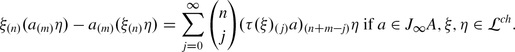  (41)

A morphism of chiral algebroids is a $\mathbb{C}$-linear map that preserves all operations and makes the following diagram commutative (cf.(12)):

(42)

Our discussion implies that if is a CDO, then is a chiral algebroid; e.g. is a chiral algebroid. We shall now explain how given a chiral algebroid to construct a CDO thus establishing, in fact, an equivalence of categories.

The meaning of Definition 5.2 is rather clear: we are given some quasiclassical data, encoded in the direct product J _∞ A ⊕ J _∞ T _A , and is its filtration quantization as . The clearest manifestation of the difference comes from the comparison of (39), which in effect says that

$$\displaystyle{[\xi _{(n)},a_{(-1)}] = (\xi _{(n)}a)_{(-1)},}$$

and a particular case of (41):

The reader is encouraged to figure out why the “quantum correction” terms, ∑ _{j < n} …, disappear in the quasiclassical limit.

The assignment is a functor from the category of CDO’s to that of chiral algebroids. It has a left adjoint, called a vertex enveloping algebra of a chiral algebroid. There is a closely related (and better known [11, 19]) concept of a vertex enveloping algebra of a vertex Lie algebra. The former is to the latter what the notion of a universal enveloping algebra of a Picard-Lie algebroid (see Sect. 2–3) is to the notion of a universal enveloping algebra of a Lie algebra. Our aim, therefore, is to chiralize the construction in Sect. 2–3.

We have seen at the bottom of page 102, that there is a forgetful functor that makes a vertex algebra into a vertex Lie algebra. This functor admits the left adjoint called the vertex enveloping algebra. Let us sketch its construction, cf. [11], 16.1.11.

Given a vertex Lie algebra L, define Lie(L) to be a linear span of symbols a _[n], a ∈ L, $n \in \mathbb{Z}$ modulo the relations

$$\displaystyle{(c_{1}a_{1}+c_{2}a_{2})_{[n]} = c_{1}(a_{1})_{[n]}+c_{2}(a_{2})_{[n]},\;(Ta)_{[n]} = -na_{[n-1]},\;c_{1},c_{2} \in \mathbb{C},a,a_{1},a_{2} \in L.}$$

Note that the last one mimics (28). Define the bracket, now mimicking (30),

$$\displaystyle{ [u_{[n]},v_{[m]}] =\sum _{ j=0}^{\infty }{n\choose j}(u_{ (\,j)}v)_{[m+n-j]}. }$$

(43)

One verifies ([11], 16.1.11 or an exercise) that this makes Lie(L) a Lie algebra. It follows from the definition that Lie(L)₊ defined to be the linear span of a _[n], a ∈ L, $n\geqslant 0$ is a Lie subalgebra. Define U ^ch L to be U(Lie(L))∕U(Lie(L)₊). Here U(. ) is the ordinary universal enveloping of a Lie algebra.

It is easy to see that the map L ⟶ Lie(L), a ↦ a _[−1], is injective, and so is the composition

$$\displaystyle{ L\longrightarrow \text{Lie}(L)\hookrightarrow U(\text{Lie}(L)) \twoheadrightarrow U(\text{Lie}(L))/U(\text{Lie}(L)_{+}) }$$

(44)

For this reason, we shall usually make no distinction between a ∈ L and a _[−1]1.

Given a ∈ L, define a field a(z) = ∑ _n a _[n] z ⁻ⁿ⁻¹; these fields clearly “generate” U ^ch(L). The Reconstruction Theorem, [11], 2.3.11 or [19], 4.5, implies that U ^ch(L) carries a vertex algebra structure. In terms of_(n)-products, it is given by a slightly tautological formula

$$\displaystyle{(\overline{a_{[-1]}})_{(n)}v = a_{[n]} \cdot v;}$$

here $\overline{a_{[-1]}}$ is the image of a _[−1] under the above composition, and ⋅ on the right means the action of Lie(L) on U(Lie(L))∕U(Lie(L)₊).

For example, $U^{ch}(J_{\infty }\mathfrak{g})$, see page 100, is the vertex algebra attached to the affine Lie algebra at level 0, $\mathfrak{g}((t))$, usually denoted by $V (\mathfrak{g})_{0}$. To shift the level one has to take $U^{ch}(\widehat{J_{\infty }\mathfrak{g}}_{(.,.)})$ and then quotient out (the ideal generated by) the element $1_{U^{ch}} - K$; notation: $V (\mathfrak{g})_{(.,.)}$. We encountered one such algebra in Sect. 4, page 94.

The constructed object, U ^ch(L), is related to a whole menagerie of multiplications,_[n] and two copies of_(n), one defined on L, another on U ^ch(L). It is a little relief to know that at least the latter two coincide when both make sense; namely,

$$\displaystyle{ u_{[n]}v = u_{(n)}v\text{ if }n\geqslant 0,u,v \in L. }$$

(45)

Indeed, we have due to (43), for $n\geqslant 0$,

$$\displaystyle{u_{[n]}v = [u_{[n]},v_{[-1]}]1 + v_{[-1]}u_{[n]}1 =\sum _{ j=0}^{\infty }{n\choose j}(u_{ (\,j)}v)_{[-1+n-j]}1 = u_{(n)}v,}$$

because by definition w _[n]1 = 0 if $n\geqslant 0$.

If is a chiral A-algebroid, then we can regard it as a vertex Lie algebra and then define . This is a vertex algebra, but it is too big to be a CDO s.t. . To see more clearly why, recall that the center of a vertex algebra V is defined to be $Z(V ) =\{ v \in V \text{ s.t. }v_{(n)}V =\{ 0\}\text{ for all }n\geqslant 0\}$. Of course, the Borcherds commutator formula (33) implies

$$\displaystyle{v \in Z(V )\Longrightarrow[v_{(n)},w_{(m)}] = 0\text{ for all }w \in V,n,m \in \mathbb{Z}.}$$

Exercise 5.6

Verify that

• (i) , 1 ∈ A;

• (ii) the center contains a polynomial ring in one variable; (Hint: consider .)

The issue we are dealing with is the same as the one we dealt with in Sect. 3: the vertex enveloping algebra does not “know” about the the “multiplicative” structure that carries; “multiplicative” in this context means “negative numbered multiplications.” This leads to the existence of a canonical ideal as follows.

Use (44) to identify with its image inside and consider the vector subspace defined as follows

The fact that the brackets (41) and (43) coincide (and (45)) implies that

(46)

Next, set . A repeated application of (46) and the normal ordering axiom (34) gives

(47)

A routine verification of these assertions is left to the reader as an exercise.

In other words, J is what is known as a vertex ideal. Denote by the vertex algebra quotient and call it the vertex enveloping algebra of a chiral algebroid.

Lemma 5.2

• (i) If is a chiral A-algebroid, then is a CDO (over A.)

• (ii) The functors

  

  are adjoints and inverses of each other.

We shall leave this lemma as an exercise.

5.1 Classification: Objects

Let us classify chiral A-algebroids; the reader is advised to compare what follows with a more familiar material of Sect. 3. Since the situation we have in mind is that of a smooth algebraic variety, we shall always assume that Ω _A is a free A-module, and if need be, the existence of a coordinate system {x _i , ∂ _i }. To make our results more explicit, we shall make one extra assumption as follows:

Recall that a vertex algebra V is called graded by conformal weight if

$$\displaystyle{V =\bigoplus _{n\in \mathbb{Z}}V _{n}\text{ s.t. }(V _{n})_{(i)}V _{m} \subset V _{n+m-i-1},1 \in V _{0},T(V _{n}) \subset V _{n+1}.}$$

(We shall often omit the descriptor “by conformal weight” if this is deemed unlikely to cause confusion.) The various examples of CDO we have seen, such as , are all graded: the degree of x _ij , ∂ _ij is − j. Thus and , the two components spanned by x _i, −1 and ∂ _i, −1; more naturally, it fits into an exact sequence

(48)

Notice that the reason Ω _A has popped up was explained in page 99: this is the A-submodule of J _∞ A that is spanned by {x _i, −1}.

The reader may be pleased to realize that the 1st time we encountered this exact sequence was (24). The familiar relations (∂ _i, −1)₍₀₎ x _i0 = 1, (∂ _i, −1)₍₁₎ x _i, −1 = 1, etc., are then an illustration of relations (V _n )_(i) V _m ⊂ V _n+m−i−1 for various n, m, i.

A similar definition applies to a chiral algebroid, and we restrict our task to classifying graded chiral algebroids.

If A has a coordinate system, then at least one chiral A-algebroid, , exists. How many more are there? Let be a chiral algebroid. A choice of a lift of an A-basis of T _A , , gives a splitting of : the map defined by

gives a splitting of (40) (Q: why?), hence an identification . With this identification, one observes that the vertex J _∞ A-module structure of is determined uniquely: it is when restricted to J _∞ A itself, by definition, and on J _∞ T _A one has using (34)

$$\displaystyle{a_{(-1)}(b_{(-1)}\partial ) = (ab)_{(-1)}\partial -\left (\sum _{n=0}^{\infty }\left (a_{ (-n-2)}b_{(n)} + b_{(-n-2)}a_{(n)}\right )\partial \right ),}$$

where the “correction terms” enclosed in brackets are predetermined: (iii) of Definition 5.2. (We omit extraneous indices and restrict ourselves to product₍₋₁₎; the reader will see that this can be done without loss of generality.)

Therefore, we have reduced the problem to

cf. (37), and observed that potentially only the vertex Lie algebra structure, $\{_{(n)},n\geqslant 0\}$, can be deformed. To begin with, notice that all the products involving J _∞ A, that is,

$$\displaystyle{_{(n)}: J_{\infty }A \otimes (J_{\infty }A \oplus J_{\infty }T_{A})\longrightarrow (J_{\infty }A \oplus J_{\infty }T_{A}),}$$

are predetermined by (iii) of Definition 5.2.

Note that none of this requires either grading or commutativity [∂ _i , ∂ _j ] = 0.

Focus on the subspace T _A ⊂ J _∞ T _A and now use the grading assumption: when restricted to T _A , of all $\{_{(n)},n\geqslant 0\}$ only two multiplications can be nonzero:

$$\displaystyle{_{(1)}: T_{A} \otimes T_{A}\longrightarrow A}$$

and

$$\displaystyle{_{(0)}: T_{A} \otimes T_{A}\longrightarrow T_{A} \oplus \varOmega _{A}.}$$

As to the former, there is no room for maneuver at all: if we replace

$$\displaystyle{\partial _{i}\text{ with }\partial _{i} - 1/2\sum _{j}\left ((\partial _{i})_{(1)}\partial _{j}\right )\omega _{j},}$$

where {ω _j } ⊂ Ω _A is the basis dual to {∂ _i } ⊂ T _A , then we obtain (check this!)

$$\displaystyle{(\partial _{i})_{(1)}\partial _{j} = 0\text{ for all }i,j,}$$

a relation we will assume throughout. If so, then an application of (34) will allow unambiguously to compute (a ₍₋₁₎ ∂ _i )₍₁₎(b ₍₋₁₎ ∂ _j ).

As to the latter, modulo Ω _A , the indicated product is nothing but the Lie bracket of vector fields, as follows from (i) of Definition 5.2. We are left, therefore, with the task of analyzing a map

$$\displaystyle{T_{A} \otimes T_{A}\longrightarrow \varOmega _{A},}$$

the composition of₍₀₎ with projection on Ω _A .

Let us put it this way: given₍₀₎: T _A ⊗ T _A ⟶ T _A ⊕Ω _A define

$$\displaystyle{_{(0)^{new}}: T_{A} \otimes T_{A}\longrightarrow T_{A} \oplus \varOmega _{A}.}$$

by the formula

$$\displaystyle{\xi _{(0)^{new}}\eta =\xi _{(0)}\eta +\alpha (\xi,\eta ),}$$

where

$$\displaystyle{\alpha: T_{A} \times T_{A}\longrightarrow \varOmega _{A}}$$

is a function of two variables. What kind of a function is it?

Exercise 5.7

• (i) Use (34) to prove that

  $$\displaystyle{(a_{(-1)}\xi )_{(0)}\eta = a_{(-1)}(\xi _{(0)}\eta )\text{ modulo predetermined terms;}}$$

• (ii) Use skew-commutativity (29) to prove that

  $$\displaystyle{\xi _{(0)}\eta = -\eta _{(0)}\xi \text{ modulo predetermined terms;}}$$

• (iii) Derive that α is A-bilinear and anti-symmetric.

In fact, more is true. Dualizing, one obtains that α can be thought of as a function

$$\displaystyle{\alpha:\; T_{A} \times T_{A} \times T_{A}\longrightarrow A,}$$

which is anti-symmetric and A-linear in the first two arguments. Notice that as a function of three variables, ξ, η, ε, it equals ε ₍₁₎(ξ ₍₀₎ η).

Exercise 5.8

• (i) Use the Borcherds commutator formula (33) to verify that

  $$\displaystyle{\epsilon _{(1)}(\xi _{(0)}\eta ) =\eta _{(1}(\epsilon _{(0)}\xi )\text{ modulo predetermined terms}.}$$

• (ii) Derive that α is totally antisymmetric and A-trilinear.

Therefore, α ∈ Ω _A ³.

Exercise 5.9

• (i) Derive from the definition of a graded chiral algebroid that part of what we called “predetermined operations,” namely

  $$\displaystyle{_{(0)}: T_{A} \otimes \varOmega _{A}\longrightarrow \varOmega _{A}\text{ and }}$$
  $$\displaystyle{_{(1)}: T_{A} \otimes \varOmega _{A}\longrightarrow A,}$$

  are the classic Lie derivative and contraction (resp.).

• (ii) Use the n = m = 0 case of ((33), which reads

  $$\displaystyle{\xi _{(0)}(\eta _{(0)}\epsilon ) -\eta _{(0)}(\xi _{(0)}\epsilon ) = (\xi _{(0)}\eta )_{(0)}\epsilon,}$$

  to prove that α must be closed: d _DR α = 0. (Hint: this is parallel but more computationally involved than Exercise 3.2; repeatedly use (i) and the Borcherds commutator formula.)

Therefore, α ∈ Ω _A ^3,cl. In fact, any closed 3-form α defines a chiral algebroid.

Lemma 5.3

Let A carry a coordinate system {x _i , ∂ _i } and α ∈ Ω _A ^3,cl . Then the assignment

$$\displaystyle{(\partial _{i})_{(n)}\partial _{j} = \left \{\begin{array}{ccc} \alpha (\partial _{i},\partial _{j},.)&\mathit{\text{ if }}&n = 0 \\ 0 &\mathit{\text{ if }}&n> 0 \end{array} \right.}$$

defines a conformally graded chiral algebroid structure on $J_{\infty }A[\partial _{in};1\leqslant i\leqslant N,n <0]^{\leqslant 1}$ . Any conformally graded chiral algebroid is isomorphic to an algebroid of this kind.

Denote the constructed chiral algebroid .

Proof

If α = 0, then we have our original chiral algebroid . It is a vertex Lie algebra, and it has a vertex Lie subalgebra $J_{\infty }A \oplus (\oplus _{in}\mathbb{C}\partial _{i,n})$. It is an extension of an abelian vertex Lie algebra $\oplus _{in}\mathbb{C}\partial _{i,n}$ by an ideal J _∞ A. The point we are trying to make is that the prescription of the lemma allows us to deform this vertex Lie algebra structure. First of all, the prescription of the lemma defines a truncated such structure on the space $J_{\infty }A \oplus (\oplus _{i}\mathbb{C}\partial _{i,-1})$. What I mean by this is that we have defined all products on this space s.t. the Borcherds commutator formula (33) holds true, but the space has been truncated and so it no longer carries the derivation T. (Indeed, expressions such as (∂ _i )_(n) a, a _(n) b, a, b ∈ J _∞ A are given to us with a _(n) b = 0, and (33) must be verified only for u, v, w being various ∂’s. In this case, the only nontrivial relation is

$$\displaystyle{\xi _{(0)}(\eta _{(0)}\epsilon ) -\eta _{(0)}(\xi _{(0)}\epsilon ) = (\xi _{(0)}\eta )_{(0)}\epsilon,}$$

and its validity is the content of Exercise 5.8.

This truncated vertex Lie algebra structure uniquely extends to the whole of $J_{\infty }A \oplus (\oplus _{in}\mathbb{C}\partial _{i,n})$: we define T by the old formula T = ∑ _i, n − nx _in ∂ _{i, −n−1}, and then use axiom (28) as motivation to define

$$\displaystyle{(T^{n}\partial _{ i})_{(m)} = (-1)^{m}m(m - 1)\cdots (m - n + 1)(\partial _{ i})_{(m-n)}.}$$

Clearly,

$$\displaystyle{(T^{n}\partial _{ i})_{(m)} = \left \{\begin{array}{ccc} (-1)^{n}n!(\partial _{i})_{(0)} & \text{ if }&n = m \\ 0 &\text{ if }& n\neq 0 \end{array} \right.,}$$

and it follows easily that with this definition the axioms of vertex Lie algebra hold true. (Think about the details!)

Denote the constructed vertex Lie algebra by .

What remains to be done is to extend the structure obtained to the “multiplicatively closed” $J_{\infty }A[\partial _{in};1\leqslant i\leqslant N,n <0]^{\leqslant 1}$. To do so, one either defines a ₍₋₁₎ ∂ _i, n to be $a\partial _{i,n} \in J_{\infty }A[\partial _{in};1\leqslant i\leqslant N,n <0]^{1}$, and then uses Definition 5.2(iv) to compute the operations, which is computationally laborious, or largely bypasses the computational hurdles by adjusting the discussion on the vertex enveloping algebra of a chiral algebroid to the present situation as follows.

First, consider the vertex enveloping algebra . Next, introduce the vector subspace

where a ₍₋₁₎ b is regarded as ab ∈ J _∞ A. We assert that

Let us prove this focusing on elements of the type a _[−1] b − a ₍₋₁₎ b. We will be repeatedly using the identification of with . We have

$$\displaystyle{\xi _{[n]}(a_{(-1)}b) =\xi _{(n)}(a_{(-1)}b) = (\xi _{(n)}a)_{(-1)}b + a_{(-1)}(\xi _{(n)}b),}$$

thanks to (31). Similarly,

$$\displaystyle\begin{array}{rcl} & & \xi _{[n]}(a_{[-1]}b) = ([\xi _{[n]},a_{[-1]}])b + a_{[-1]}\xi _{[n]}b =\sum _{ j=0}^{\infty }{n\choose j}(\xi _{ (\,j)}a)_{[-1+n-j]}b + a_{(-1)}(\xi _{(n)}b) = {}\\ & & \sum _{j=0}^{n-1}{n\choose j}(\xi _{ (\,j)}a)_{(-1+n-j)}b + (\xi _{(n)}a)_{[-1]}b + a_{(-1)}(\xi _{(n)}b) = (\xi _{(n)}a)_{[-1])}b + a_{(-1)}(\xi _{(n)}b),{}\\ \end{array}$$

the terms (ξ _( j) a)_(−1+n−j) b, $0\leqslant j\leqslant n - 1$ vanishing, because ξ _( j) a ∈ J _∞ A and (J _∞ A)_(i) J _∞ A = {0} if $i\geqslant 0$. By definition

$$\displaystyle{\xi _{[n]}(a_{(-1)}b) -\xi _{[n]}(a_{[-1]}b) \in I,}$$

as desired. As in (47), is a vertex ideal. It is easy to understand (do this!) that the quotient is a CDO. The component is the desired chiral algebroid. □

5.2 Classification: Morphisms

Since by construction each (i.e., the algebroid constructed in Lemma 5.3) comes equipped with a splitting, , definition (42) implies that a graded morphism

is determined by a map

$$\displaystyle{\beta: T_{A}\longrightarrow \varOmega _{A}}$$

s.t. f(ξ) = ξ + β(ξ). As before, it is convenient to dualize and introduce

$$\displaystyle{\beta: T_{A} \otimes T_{A}\longrightarrow A}$$

s.t. f(ξ) = ξ + β(ξ, . ). The interested reader may be anticipating what is to follow.

Exercise 5.10

Verify that β must be A-linear and antisymmetric. (Remark: we have used normalization (∂ _i )₍₁₎ ∂ _j = 0; this is the reason why β must be antisymmetric.)

Therefore, β ∈ Ω _A ².

Lemma 5.4

where the morphism attached to β is defined by

$$\displaystyle{T_{A}\xi \mapsto \xi +\beta (\xi,.).}$$

Proof

This is in the spirit of Sect. 3 and Exercise 5.9, but less laborious, and we shall go over some details. We need to compare f(ξ ₍₀₎ η) and f(ξ)₍₀₎ f(η), ξ, η ∈ T _A . We have

$$\displaystyle{f(\xi _{(0)}\eta ) = \cdots \alpha _{1}(\xi,\eta,.) +\beta ([\xi,\eta ],.),}$$

$$\displaystyle\begin{array}{rcl} f(\xi )_{(0)}f(\eta )& =& (\xi +\beta (\xi,.))_{(0)}(\eta +\beta (\eta,.)) = \cdots +\alpha _{2}(\xi,\eta,.) +\xi _{(0)}\beta (\eta,.) +\beta (\xi,.)_{(0)}\eta {}\\ & =& \cdots +\alpha _{2}(\xi,\eta,.) +\xi _{(0)}\beta (\eta,.) -\eta _{(0)}\beta (\xi,.) + d_{DR}\beta (\xi,\eta ), {}\\ \end{array}$$

where ⋯ stands for the terms uniquely determined by the axioms. (Note that the last equality uses the skew-symmetry (29) as follows:

$$\displaystyle{\beta (\xi,.)_{(0)}\eta = -\eta _{(0)}\beta (\xi,.) + T(\eta _{(1)}\beta (\xi,.)).)}$$

To compare the two 1-forms we have to evaluate them on an arbitrary ζ ∈ T _A and subtract from one another; in vertex algebra terms to evaluate means to apply ζ ₍₁₎. We have

$$\displaystyle\begin{array}{rcl} & & \zeta _{(1)}(\,f(\xi )_{(0)}f(\eta )) -\zeta _{(1)}f(\xi _{(0)}\eta ) =\alpha _{2}(\xi,\eta,\zeta ) -\alpha _{1}(\xi,\eta,\zeta ) + {}\\ & & \zeta _{(1)}\xi _{(0)}\beta (\eta,.) -\zeta _{(1)}\eta _{(0)}\beta (\xi,.) +\zeta _{(1)}d_{DR}\beta (\xi,\eta ) -\zeta _{(1)}\beta ([\xi,\eta ],.) {}\\ \end{array}$$

The R.H.S. must be zero. To evaluate the R.H.S., use the Borcherds commutator formula, e.g.,

$$\displaystyle{\zeta _{(1)}\xi _{(0)} =\xi _{(0)}\zeta _{(1)} + (\zeta _{(0)}\xi )_{(1)} + (\zeta _{(1)}\xi )_{(0)},}$$

and then the fact (Exercise 5.9(i)) that ξ ₍₀₎ is the Lie derivative along ξ and ξ ₍₁₎ is the contraction with ξ. We obtain

$$\displaystyle\begin{array}{rcl} & & \alpha _{1}(\xi,\eta,\zeta ) -\alpha _{2}(\xi,\eta,\zeta ) = {}\\ & & \xi \beta (\eta,\zeta ) -\eta \beta (\xi,\zeta ) +\zeta \beta (\xi,\eta ) -\beta ([\xi,\eta ],\zeta ) +\beta ([\xi,\zeta ],\eta ) -\beta ([\eta,\zeta ],\xi ), {}\\ \end{array}$$

which by definition is the desired

$$\displaystyle{\alpha _{1}(\xi,\eta,\zeta ) -\alpha _{2}(\xi,\eta,\zeta ) = d_{DR}\beta (\xi,\eta,\zeta ).}$$

□

5.3 Classification: Synthesis

All of this is delightfully analogous to Sect. 3—analogous in a nontrivial manner, as the dimension has gone up by 1. We leave it to the reader to push the analogy a little further and to define the category Ω _A ^{[2,3 >} with objects {α ∈ Ω _A ^3,cl} and morphisms Hom(α ₁, α ₂) = { β ∈ Ω _A ² s.t. α ₁ −α ₂ = d _DR β}; then verify that Ω _A ^{[2,3 >} is an abelian group in categories, and that the category of graded chiral A-algebroids, hence of CDOs over A, is an Ω _A ^{[2,3 >}-torsor.

What this means geometrically is that on any smooth algebraic variety X there is a sheaf of groupoids bound by the complex Ω _X ² → Ω _X ^3,cl. In particular, given a CDO defined over an open U ⊂ X and a closed 3-form α ∈ Ω _X ^3,cl(U) we have a naturally defined CDO over U, see the line that follows Lemma. 5.3.

We shift the cohomological degree so as to place Ω _X ² in degree 0 and consider the (hyper)cohomology H ^•(X, Ω _X ² → Ω _X ^3,cl). The cohomology groups have usual interpretations: if the category of globally defined CDOs is nonempty, then the set of isomorphism classes of such is H ¹(X, Ω _X ² → Ω _X ^3,cl); H ⁰(X, Ω _X ² → Ω _X ^3,cl) is the group of automorphisms of any CDO if, again, one exists. All of this is not really different from Sect. 3, but here is the point: is characterized by, well, its characteristic class , which is an element of H ²(X, Ω _X ² → Ω _X ^3,cl). This class is an obstruction to the existence of a globally defined CDO: if , then no such CDO exists. The class was computed in [17] to the effect that it equals the 2nd component of the Chern character:

A more general result can be found in [7]. We shall leave this computation out, referring the reader to loc. cit., but give a bit of an insight here.

First of all, the definition of the characteristic class. Cover X by affine subset {U _a } along with a choice of coordinate system {x _i ^a, ∂ _i ^a}. We have a description of the category of CDOs over each U _a , and we can make a choice of an object; say, , as in Sect. 4. Over an intersection U _a ∩ U _b we have two sheaves, and and we attempt to find an isomorphism

This isomorphism is not only a vertex algebra morphism, but it must satisfy the definition of the category of chiral algebroids, (42); namely, the induced maps

must be identities, as both of the former spaces are equal to and of the latter to . The result of implementing this is not quite what we wanted, but an isomorphism

for some α _ab ∈ Ω _X ^3,cl(U _a ∩ U _b ). We shall say a few words on how these α’s are computed below.

On a triple intersection, U _a ∩ U _b ∩ U _c , an appropriate composition of f _•’s gives an isomorphism

hence, see Lemma 5.4, a form β _abc ∈ Ω _X ²(U _a ∩ U _b ∩ U _c ) s.t. d _DR β _abc = α _bc −α _ac + α _ab .

We have thus obtained two sets {α _ab } and {β _abc } s.t.

$$\displaystyle{d_{DR}\{\beta _{abc}\} = d_{\check{\mbox{C}}}\{\alpha _{ab}\}.}$$

It is not hard to see that d _Č{β _abc } = 0—think about it(!) and then recall that d _DR {α _ab } = 0. This means that the pair ({α _ab }, {β _abc }) is a cocycle of an obviously defined Čech-De Rham bi-complex C ^•(X, Ω _X ² → Ω _X ^3,cl). Computing we have made various choices; other choices will replace the cocycle with a cohomologous one, hence a well-defined element of H ²(X, Ω _X ² → Ω _X ^3,cl).

To conclude, a few promised words on the computation of the α’s. We have two copies of the same vertex algebra attached to various coordinate systems, and . The desired map must send³

$$\displaystyle{(\partial _{i}^{a})_{ (-1)}1\mapsto (\frac{\partial x_{s}^{b}} {\partial x_{i}^{a}})_{(-1)}(\partial _{s}^{b})_{ (-1)}1 + \cdots \,,}$$

⋯ meaning the terms we have control over. If we let ⋯ = 0, shall we obtain a morphism? This situation is familiar from as early as Sect. 4: compute

$$\displaystyle{\left ((\frac{\partial x_{s}^{b}} {\partial x_{i}^{a}})_{(-1)}(\partial _{s}^{b})_{ (-1)}1\right )_{(1)}\left ((\frac{\partial x_{s}^{b}} {\partial x_{j}^{a}})_{(-1)}(\partial _{s}^{b})_{ (-1)}1\right )}$$

and if it is nonzero add to the morphism an appropriate 1-form, γ _i , to ensure that this product vanishes. Then compute

$$\displaystyle{\left (\left ((\frac{\partial x_{s}^{b}} {\partial x_{i}^{a}})_{(-1)}(\partial _{s}^{b})_{ (-1)} +\gamma _{i}\right )1\right )_{(0)}\left (\left ((\frac{\partial x_{s}^{b}} {\partial x_{j}^{a}})_{(-1)}(\partial _{s}^{b})_{ (-1)} +\gamma _{j}\right )1\right ).}$$

The result will automatically be α _ab (∂ _i ^a, ∂ _j ^b, . ) for some α _ab , Sect. 5.1, as desired. We hope this may serve as a useful guide to [17].

6 Further Examples

This section contains some material that I really did not have time for in class. It is included for the sake of completeness and regarded as a review, except perhaps for Sect. 6.1.1, which I hope is a useful illustration of the ideas that appeared above.

6.1 Homogeneous Spaces

6.1.1 CDO on G

This is based on [15]. Let $\mathfrak{g}$ be a finite dimensional, simple Lie algebra, G the corresponding algebraic group. G operates on itself by left multiplication, which gives a Lie algebra morphism

The tangent bundle TG is trivial, and so and the category of CDOs over G is nonempty. Next, G being affine,

$$\displaystyle{H^{1}(G,\varOmega _{ G}^{2} \rightarrow \varOmega _{ G}^{3,cl}) =\varGamma (G,\varOmega ^{3,cl})/d_{ DR}\varGamma (G,\varOmega ^{2})\mathop{\longrightarrow }\limits^{ \sim } \mathbb{C},}$$

with basis a G-invariant form ω s.t. ω(x, y, z) = (x, [y, z]), where $x,y,z \in j_{l}(\mathfrak{g})$, (. , . ) a choice of an invariant inner product on $\mathfrak{g}$, [. , . ] the Lie bracket on $\mathfrak{g}$.

According to our classification, Sect. 5.3, the isomorphism classes of CDOs over G form a $\mathbb{C}$-torsor. In fact, it is easy and instructive to construct a universal 1-dimensional family of these CDOs.

Lemma 5.3 asserts that such quantization is possible if T _A has an abelian basis. Some further thought shows that the abelian condition is inessential and can be weakened. To begin with, assume given a Lie algebra morphism

$$\displaystyle{\mathfrak{a}\longrightarrow T_{A}.}$$

This lets $\mathfrak{a}$ act on A by derivations and we obtain $A \rtimes \mathfrak{a}$, an extension of $\mathfrak{a}$ by an abelian ideal A

This can be chiralized: let $J_{\infty }\mathfrak{a} = \mathbb{C}[T]\mathfrak{a}$, which is a vertex Lie algebra, see page 100, for the definition, and then J _∞ A is a $J_{\infty }\mathfrak{a}$-module. We thus obtain a vertex Lie algebra $J_{\infty }A \rtimes J_{\infty }\mathfrak{a}$, an extension of $J_{\infty }\mathfrak{a}$ by J _∞ A. This gives us a vertex Poisson algebra $J_{\infty }A \otimes S^{\bullet }J_{\infty }\mathfrak{a}$ (the vertex Poisson algebra $S^{\bullet }J_{\infty }\mathfrak{a}$ first appeared in page 101) along with a vertex Poisson algebra morphism:

$$\displaystyle{J_{\infty }A \otimes S^{\bullet }J_{\infty }\mathfrak{a}\longrightarrow S^{\bullet }J_{\infty }T_{A}.}$$

The domain of this map can be quantized, and this is the point. Namely, consider $U^{ch}(J_{\infty }A \rtimes J_{\infty }\mathfrak{a})$, and then quotient out by the vertex ideal generated by the elements $1_{A} - 1_{U^{ch}}$, a _[−1] b − a ₍₋₁₎ b, a, b ∈ J _∞ A—exactly as in the proof of Lemma 5.3. Denote the vertex algebra thus obtained by .

is filtered, and its graded object is exactly $J_{\infty }A \otimes S^{\bullet }J_{\infty }\mathfrak{a}$.

Now assume that the map $A \otimes \mathfrak{a} \rightarrow T_{A}$, which is induced by the above $\mathfrak{a}\longrightarrow T_{A}$, is an isomorphism. It follows that the map $J_{\infty }A \otimes S^{\bullet }J_{\infty }\mathfrak{a}\longrightarrow S^{\bullet }J_{\infty }T_{A}$ is also an isomorphism, hence is a quantization of S ^• J _∞ T _A .

This construction can be deformed. Namely, consider a central extension of vertex Lie algebras,

$$\displaystyle{0\longrightarrow \mathbb{C} \cdot 1_{L}\longrightarrow L\longrightarrow J_{\infty }\mathfrak{a}\longrightarrow 0.}$$

This also gives us an extension $J_{\infty }A \rtimes L$ and a vertex Poisson algebra morphism

$$\displaystyle{J_{\infty }A \otimes S^{\bullet }L\longrightarrow S^{\bullet }J_{\infty }T_{A}.}$$

Defining as above to be U ^ch(J _∞ A ⊗ S ^• L) modulo the ideal generated by $1_{A} - 1_{U^{ch}}$, a _[−1] b − a ₍₋₁₎ b AND 1 _A − 1 _L gives us a quantization of S ^• J _∞ T _A —again if $A \otimes \mathfrak{a} \rightarrow T_{A}$ is an isomorphism.

This is exactly the set-up of the group G, where $\mathfrak{a}$ is replaced with $\mathfrak{g}$, $\mathfrak{a} \rightarrow T_{A}$ with and L with the central extension $\widehat{J_{\infty }\mathfrak{g}}_{(.,.)}$. The result is a family of CDOs, , along with the tautological embedding

the vertex algebra $V (\mathfrak{g})_{(.,.)}$ was defined in Sect. 5.

One remarkable fact about is that the action by right translations (discovered in [2])

also chiralizes: there is a diagram of vertex algebra embeddings

Note that the “right” action requires a change of level from (. , . ) to the dual (. , . )^∨.

The CDO has found nontrivial applications to geometry and representation theory, [2, 13].

6.1.2 Flag Manifolds and Base Affine Spaces

The CDO on $\mathbb{C}\mathbb{P}^{1}$ constructed by hand in Sect. 4 owes its existence to the fact that $\text{dim}\mathbb{C}\mathbb{P}^{1} = 1$ and so the obstruction, Sect. 5.3, vanishes for the trivial dimensional reason. Likewise, $H^{1}(\mathbb{C}\mathbb{P}^{1},\varOmega _{v}^{2} \rightarrow \varOmega _{\mathbb{C}\mathbb{P}^{1}}^{3,cl}) = 0$, and so that sheaf is unique up to isomorphism.

The dimensional argument does not work for $\mathbb{C}\mathbb{P}^{2}$, and indeed there are no CDOs on $\mathbb{C}\mathbb{P}^{n}$ for any n > 1. The appropriate generalization of $\mathbb{C}\mathbb{P}^{1}$ for a simple G is the flag manifold, where there is a unique up to isomorphism CDO , [15]. A simple way to construct it is to use the ideas of Hamiltonian reduction.

Consider a chain N ⊂ B ⊂ G, where N is the maximal unipotent and B the Borel subgroups.

For any smooth X, T ^∗ X is simplectic.

The action of G (by left translations) on T ^∗ G is simplectic; the same applies to any subgroup of G.

The simplectic manifolds T ^∗(G∕N) and T ^∗(G∕B) are, in fact, Hamiltonian reductions of T ^∗ G w.r.t. N (B resp.)

This has a chiral analogue due to the pioneering work of Feigin [10]. Consider , Sect. 6.1.1. It carries two actions of the affine Lie algebra $\widehat{\mathfrak{g}}$. Pick the one coming from j _r ^ch and pull it back w.r.t. $\mathfrak{n}((t))\hookrightarrow \widehat{\mathfrak{g}}$. A sheaf version of Feigin’s semi-infinite cohomology [10]⁴ will give a sheaf on G and then the push-forward , where π: G → G∕N. It is not hard to see that is a family of CDOs on the base affine space G∕N, [15]. The passage to the cohomology destroys j _r ^ch, but j _l ^ch survives and we obtain a $\widehat{\mathfrak{g}}$-structure

The flag manifold G∕B is dealt with similarly, except that in this case the relevant subgroup B is not contractible, $\mathfrak{b}((t))$ undergoes a central extension, and the cohomology does not quite make sense. To straighten things out, one has to replace the absolute semi-infinite cohomology with the relative, and specialize the central charge to the critical one, [15]. The result is a unique CDO on G∕B, , along with a morphism

This is a proper generalization of Sect. 4. The generalization of Theorem 4.1 is the following result proved in [1]:

where W ⁽ⁱ⁾ is the set of length i elements of the Weyl group W.

Note that if we let U ⊂ G∕B be the big cell, then is, by definition, the Wakimoto module, [12]. In fact, the approach sketched here is a way to introduce the Wakimoto module independent of [12].

6.2 Chiral De Rham and String Theory

The story told above has a straightforward super-analogue: one should simply deal with a sheaf of vertex superalgebras over a supervariety. Unfortunately, the only case that was treated in some detail is that of the supervariety , where is a vector bundle. What this really means is that the structure sheaf in question is the supercommutative algebra . In this case, [16], the characteristic class of the arising groupoid of categories over X is . In particular, if , then the characteristic classes vanishes and there arises a category of superCDOs over any smooth X. What is striking, however, is that amongst those various CDOs over various X there is a universal one. More precisely, for each smooth(purely even) X, there is a doubly graded sheaf of vertex superalgebras over X, to be denoted Ω _X, • ^ch, •. It is universal in that for each étale f: X → Y, there is a vertex superalgebra morphism f ⁻¹ Ω _X, • ^ch, • → Ω _Y, • ^ch, • that satisfies an easy to work out cocycle condition. This sheaf satisfies various other favorable properties; e.g. its degree 0 component is the usual De Rham Ω _X ^•; it carries a differential—so to say, a chiral De Rham differential—s.t. the embedding Ω _X ^• → Ω _X, • ^ch, • is a quasiisomorphism. This sheaf was constructed by hands in [25] and called the chiral De Rham complex; this is where the CDO story began.

L. Borisov wrote a series of papers, starting with the strikingly original [4], linking and applying Ω _X, • ^ch, • to mirror symmetry on toric varieties. A relation of Ω _X, • ^ch, • to the concept of elliptic genus is discussed in [8]. Incidentally, an analogue of this concept to the purely even , the Euler character , which appeared in Sect. 4 in an example, is essentially the Witten genus [9].

We will conclude by mentioning that this theory has been analyzed from various physics viewpoints by A. Kapustin, N. Nekrasov, and E. Witten in [22, 26, 28].

References

T. Arakawa, F. Malikov, A chiral Borel-Weil-Bott theorem. Adv. Math. 229(5), 2908–2949 (2012)
S. Arkhipov, D. Gaitsgory, Differential operators on the loop group via chiral algebras. Int. Math. Res. Not. 2002(4), 165–210 (2002)
R.E. Borcherds, Vertex algebras, Kac-Moody algebras, and the Monster. Proc. Natl. Acad. Sci. 83(10), 3068–3071 (1986)
L. Borisov, Vertex algebras and mirror symmetry. Commun. Math. Phys. 215(3), 517–557 (2001)
A. Beilinson, J. Bernstein, Localisation de \(\mathfrak{g}\)-modules. CR Acad. Sci. Paris Se’r. I Math. 292(1), 15–18 (1981 in French)
A. Beilinson, J. Bernstein, A proof of Jantzen conjectures, in I.M. Gelfand Seminar, Advances in Soviet Mathematics, Part 1, vol. 16 (American Mathematical Society, Providence, RI, 1993), pp. 1–50
A. Beilinson, V. Drinfeld, Chiral Algebras. American Mathematical Society Colloquium Publications, vol. 51 (American Mathematical Society, Providence, RI, 2004), vi+375 pp., ISBN: 0-8218-3528-9
L. Borisov, A. Libgober, Elliptic genera of toric varieties and applications to mirror symmetry. Inv. Math. 140(2), 453–485 (2000)
K. Costello, A geometric construction of the Witten genus, I, in Proceedings of the International Congress of Mathematicians, vol. II (Hindustan Book Agency, New Delhi, 2010), pp. 942–959
B. Feigin, Semi-infinite homology of Lie, Kac-Moody and Virasoro algebras. Uspekhi Mat. Nauk 39(2), 155–156 (1984 in Russian)
E. Frenkel, D. Ben-Zvi, in Vertex Algebras and Algebraic Curves, 2nd edn. Mathematical Surveys and Monographs, vol. 88 (American Mathematical Society, Providence, RI, 2004)
B. Feigin, E. Frenkel, Representations of affine Kac-Moody algebras and bosonization, in V. Knizhnik Memorial Volume, ed. by L. Brink, D. Friedan, A.M. Polyakov, (World Scientific, Singapore, 1990), pp. 271–316
E. Frenkel, D. Gaitsgory, Localization of \(\mathfrak{g}\)-modules on the affine Grassmannian, Ann. Math. 170(3), 1339–1381 (2009)
I. Frenkel, Y. Zhu, Vertex operator algebras associated to representations of affine and Virasoro algebras. Duke Math. J. 66(1), 123–168 (1992)
V. Gorbounov, F. Malikov, V. Schechtman, Gerbes of chiral differential operators over homogeneous spaces. Int. J. Math. Math. Sci. 26(2) 83–106 (2001)
V. Gorbounov, F. Malikov, V. Schechtman, Gerbes of chiral differential operators. III. The orbit method in geometry and physics (Marseille, 2000), Progress in Mathematics, vol. 213 (Birkhäuser Boston, Boston, MA, 2003), pp. 73–100
V. Gorbounov, F. Malikov, V. Schechtman, Gerbes of chiral differential operators. II. Vertex algebroids. Invent. Math. 155(3), 605–680 (2004)
J. Humphreys, Representations of Semisimple Lie Algebras in the BGG Category
. Graduate Studies in Mathematics, vol. 94 (American Mathematical Society, Providence, RI, 2008)
V. Kac, Vertex Algebras for Beginners. University Lecture Series, vol. 10 (American Mathematical Society, Providence, RI, 1997). viii+141 pp., ISBN: 0-8218-0643-2
M. Kapranov, E. Vasserot, Vertex algebras and the formal loop space. Publ. Math. Inst. Hautes Études Sci. 100, 209–269 (2004)
M. Kapranov, E. Vasserot, Formal loops. II. A local Riemann-Roch theorem for determinantal gerbes. Ann. Sci. École Norm. Sup. (4) 40(1), 113–133 (2007)
A. Kapustin, Chiral de Rham complex and the half-twisted sigma-model, preprint, hep-th/0504074
B. Kostant, Lie group representations on polynomial rings. Am. J. Math. 85(3), 327–404 (1963)
F. Malikov, Verma modules over rk2 Kac-Moody algebras. Algebra i analiz n. 2 2, 65–84 (1990). English translation: Leningrad Math. J. 2, 269–286 (1991)
F. Malikov, V. Schechtman, A. Vaintrob, Chiral de Rham complex. Commun. Math. Phys. 204 (1999), 439–473
N. Nekrasov, Lectures on curved beta-gamma systems, pure spinors, and anomalies, preprint, arXiv:hep-th/0511008
M. Wakimoto, Fock repesentations of affine Lie algebra A 1 (1). Commun. Math. Phys. 104 (1986), 605–609
E. Witten, Two-dimensional models with (0,2) supersymmetry: perturbative aspects. Adv. Theor. Math. Phys. 11(1), 1–63 (2007), hep-th/0504078
Author information
Authors and Affiliations
Corresponding author
Editor information
Editors and Affiliations
Rights and permissions
Copyright information
© 2017 Springer International Publishing AG
About this chapter
Cite this chapter
Malikov, F. (2017). An Introduction to Algebras of Chiral Differential Operators. In: Callegaro, F., Carnovale, G., Caselli, F., De Concini, C., De Sole, A. (eds) Perspectives in Lie Theory. Springer INdAM Series, vol 19. Springer, Cham. https://doi.org/10.1007/978-3-319-58971-8_2
Download citation
DOI: https://doi.org/10.1007/978-3-319-58971-8_2
Published:
Publisher Name: Springer, Cham
Print ISBN: 978-3-319-58970-1
Online ISBN: 978-3-319-58971-8
eBook Packages: Mathematics and StatisticsMathematics and Statistics (R0)